Statistical Inference on the Canadian Middle Class

Abstract

Conventional wisdom says that the middle classes in many developed countries have recently suffered losses, in terms of both the share of the total population belonging to the middle class, and also their share in total income. Here, distribution-free methods are developed for inference on these shares, by means of deriving expressions for their asymptotic variances of sample estimates, and the covariance of the estimates. Asymptotic inference can be undertaken based on asymptotic normality. Bootstrap inference can be expected to be more reliable, and appropriate bootstrap procedures are proposed. As an illustration, samples of individual earnings drawn from Canadian census data are used to test various hypotheses about the middle-class shares, and confidence intervals for them are computed. It is found that, for the earlier censuses, sample sizes are large enough for asymptotic and bootstrap inference to be almost identical, but that, in the twenty-first century, the bootstrap fails on account of a strange phenomenon whereby many presumably different incomes in the data are rounded to one and the same value. Another difference between the centuries is the appearance of heavy right-hand tails in the income distributions of both men and women.

1. Introduction

There has been much discussion in many countries about the fate of the middle class, variously defined. It appears clearly that middle classes in different developed countries have had rather different experiences; in particular, the case of the USA, about which a lot has been written, for instance, Heathcote et al. (2010), is in no way typical or representative. Canada shares a long border with the USA, and has a culture more similar to the American one than any other country, but it maintains a separate identity, and differs from the US markedly on matters of social security and immigration. Nevertheless, a couple of decades ago, it was pointed out by Foster and Wolfson (2010) that, in both countries, a decline of the middle class had led to a polarisation of the income distribution. In Canada specifically, the situation is reviewed by Brzozowski et al. (2010), for inequality not only of income, but also of wealth and consumption. For the USA, an early article by Wolfson (1994) discusses polarisation, while Wolff (2013) describes the fate of the wealth of the middle class following the crisis of 2008. Some recent trends in income inequality in different European regions have been analysed by Castells-Quintana et al. (2015).

The study of income inequality, and its effects on growth, social stability, and many other features of society, started more than half a century ago, with Kuznets (1955). A landmark contribution to the measurement of income inequality was Atkinson (1970). A useful article is Cowell (1999), which appears in the Handbook of Income Inequality Measurement, and contains many chapters on different aspects of the topic, some purely theoretical, such as the seminal contributions of Blackorby et al. (1999). An interesting recent paper, Ryu (2013), develops a sort of inverted Gini index that emphasises the distribution of the poor, and describes ways of estimating income distributions based on the principle of maximum entropy.

The Canadian Liberal federal government elected in late 2015 has made a point of trying to improve the lot of the Canadian middle class, claiming, no doubt with some justice, that the share of the middle class, however defined, has declined over the last several decades, in terms of both the share of the population belonging to the middle class, and also its share in total national income.

Beach (2016), in his presidential address to the Canadian Economics Association, drew a wide-ranging portrait of the evolution of Canadian middle-class fortunes since the 1970s. His analysis tries to understand the different mechanisms that have shaped the economic environment in which this evolution has taken place. He provides abundant statistical information on earnings in Canada, duly separating the two sexes in his analysis, given that their position in the labour market has changed very considerably in the last fifty years.

The aim of this paper is to bring some formal statistical analysis to bear on the Canadian census data. The work of Davidson and Duclos1, found in Davidson and Duclos (1997) and Davidson and Duclos (2000), introduced a set of statistical procedures that permit distribution-free inference on income data, many of which can be used directly for the analysis in this paper. Some extensions of their methodology are developed here to deal with the specific problems addressed.

Formal analysis requires a formal definition of the middle class. An ideal definition would have to be based on all sorts of socioeconomic characteristics of individuals and households, but such a thing is well outside the scope of this paper. Instead, we consider definitions based solely on individual income. Usually different segments of the income distribution are defined by use of quantiles, and income data are sometimes grouped by deciles or vigintiles. Thus, a possible definition of the middle class could be those households or individuals whose incomes lie between the second decile and the eighth. Another approach would be to define the upper and lower bounds of middle-class incomes as multiples of the mean or median income. However, given the stylised fact that the recent changes in income inequality in most developed countries have favoured the rich and the super-rich, use of the mean as a criterion for defining income classes is likely to distort inference. It is easy to see that a substantial increase in the income of the upper 10% of the distribution, with no changes for the lower 90%, leads to an increase in mean income and no change in the median. Similarly, quantile-based definitions of the middle class are unaffected by an increase in the income of the rich and only the rich.

If the middle class is defined as the set of individuals with incomes between the $p_{\mathrm{lo}}$ quantile of the income distribution and the $p_{\mathrm{hi}}$ quantile, where a possible choice might be $p_{\mathrm{lo}}=0.2$ and $p_{\mathrm{hi}}=0.8$, it is not possible to measure changes in the population share of the middle class, because this share is always just $p_{\mathrm{hi}}-p_{\mathrm{lo}}$. It remains possible to measure changes in the income share.

In the next section, distribution-free plug-in estimators are presented for the population and income shares of the middle class, according to three different sorts of definition of the middle class—based on the median income, based on the mean income, and based on quantiles of the income distribution. These estimators are shown to be consistent and asymptotically normal, and feasible estimators are given for the asymptotic variance. Then, in Section 3, the evolution over time of the middle-class shares in Canada is analysed using census data from the 1971 census to that in 2006. Section 4 concludes.

2. Asymptotic Analysis

We begin with a definition of the middle class as the section of the population with incomes between a fraction a of median income and a multiple b of it. Typically, we might have $a=0.5$ and $b=1.5$. It is desired to estimate the size of this section of the population, and also to estimate its share in total income. Other definitions will be considered later.

2.1. Definition in Terms of the Median

Let m denote median income. Then, the proportion of the population considered to be middle class is $F\left(bm\right)-F\left(am\right)$, where F is the cumulative distribution function (CDF) of income in the population. To estimate this quantity based on a random sample of size N, it is necessary to have an estimate of F, i.e., $\widehat{F}$, from which an estimate of m may be deduced, or else obtained directly using order statistics, by use of the formula

$$\widehat{m}=\left\{\begin{array}{cc}{y}_{(n+1)}\hfill & \mathrm{if}N=2n+1\left(N\mathrm{odd}\right)\hfill \\ (y_{\left(n\right)}+y_{(n+1)})/2\hfill & \mathrm{if}N=2n\left(N\mathrm{even}\right)\hfill \end{array}\right.$$

The natural choice for $\widehat{F}$ is the empirical distribution function (EDF):

$$\widehat{F}\left(y\right)=\frac{1}{N}\sum _{i=1}^N\mathrm{I}(y_i\le y),$$

(1)

where the $y_i$ are the incomes observed in the sample, and I is the indicator function, equal to 1 when its argument is true, to 0 otherwise. If $PS$ denotes the share of the middle class in the whole population, then it can be estimated by

$$\widehat{PS}=\widehat{F}\left(b\widehat{m}\right)-\widehat{F}\left(a\widehat{m}\right)$$

(2)

The income share, i.e., $IS$, that accrues to the middle class is by definition given by

$${\int }_{am}^{bm}y\mathrm{d}F\left(y\right)$$

divided by the mean income, denoted by $\mu$, and equal to ${\int }_0^{\infty }y\mathrm{d}F\left(y\right)$. The plug-in estimator of $\mu$ is

$$\widehat{\mu }={\int }_0^{\infty }y\mathrm{d}\widehat{F}\left(y\right)=\frac{1}{N}\sum _{i=1}^N{y}_i.$$

Consequently, a suitable estimate of $IS$ is

$$\widehat{IS}\equiv \frac{1}{\widehat{\mu }}{\int }_{a\widehat{m}}^{b\widehat{m}}y\mathrm{d}\widehat{F}\left(y\right).$$

(3)

For asymptotic statistical inference, we need estimates of the asymptotic covariance matrix of $(\widehat{PS},\widehat{IS})$. Consider first the asymptotic variance of $\widehat{PS}$, which is by definition the variance of the limit in distribution as $N\to \infty$ of $N^{1/2}(\widehat{PS}-PS)$. We have

$$\widehat{PS}-PS=\widehat{F}\left(b\widehat{m}\right)-F\left(bm\right)-(\widehat{F}\left(a\widehat{m}\right)-F\left(am\right)).$$

(4)

Now

$$\widehat{F}\left(b\widehat{m}\right)-F\left(bm\right)={\int }_0^{bm}\mathrm{d}(\widehat{F}-F)\left(y\right)+{\int }_{bm}^{b\widehat{m}}\mathrm{d}F\left(y\right)+{\int }_{bm}^{b\widehat{m}}\mathrm{d}(\widehat{F}-F)\left(y\right).$$

The first two terms on the right-hand side are of order $N^{-1/2}$ if, as we can reasonably assume, things are regular enough for both $(\widehat{F}-F)\left(y\right)$ and $\widehat{m}-m$ to be of that order. The last term, on the other hand, is of order $N^{-1}$, and so can be dropped for the purposes of asymptotic analysis. The first term is

$$\frac{1}{N}\sum _{i=1}^N\left[\mathrm{I}(y_i\le bm)-F\left(bm\right)\right],$$

(5)

and the second is

$$bf\left(bm\right)(\widehat{m}-m)+O\left(N^{-1}\right),$$

(6)

where $f=F^{\prime }$ is the density function. By the Bahadur (1966) almost-sure representation of quantiles, we have

$$\widehat{m}-m=-\frac{1}{Nf\left(m\right)}\sum _{i=1}^N[\mathrm{I}(y_i<m)-\frac{1}{2}]+O(N^{-3/4}{(logN)}^{1/2}{(loglogN)}^{1/4}).$$

(7)

From (4), (5), (6), and (7), we conclude that

$$\begin{array}{cc}\hfill N^{1/2}(\widehat{PS}-PS)=N^{-1/2}\sum _{i=1}^N& \left\{\right[\mathrm{I}(am\le y_i\le bm)-\left(F\left(bm\right)-F\left(am\right)\right)]\hfill \\ & -\frac{bf\left(bm\right)-af\left(am\right)}{f\left(m\right)}\left[\mathrm{I}(y_i<m)-\frac{1}{2}\right]\}+o_p\left(1\right).\hfill \end{array}$$

It is convenient to make the following definition:

$$u_i=\mathrm{I}(am<y_i<bm)-\frac{bf\left(bm\right)-af\left(am\right)}{f\left(m\right)}\mathrm{I}(y_i<m).$$

(8)

Since the $y_i$ are IID, as elements of a random sample, so are the $u_i$, so that, to leading order asymptotically,

$$N^{1/2}(\widehat{PS}-PS)=N^{-1/2}\sum _{i=1}^N\left(u_i-\mathrm{E}\left(U\right)\right),$$

(9)

where U denotes a random variable that has the distribution of which the $u_i$ are IID realisations. We may therefore apply the central-limit theorem to show that $N^{1/2}(\widehat{PS}-PS)$ is asymptotically normal, with expectation zero and variance equal to that of U. If we make the definition

$${\widehat{u}}_i=\mathrm{I}(a\widehat{m}<y_i<b\widehat{m})-\frac{b\widehat{f}\left(b\widehat{m}\right)-a\widehat{f}\left(a\widehat{m}\right)}{\widehat{f}\left(\widehat{m}\right)}\mathrm{I}(y_i<\widehat{m}),$$

where the density estimate $\widehat{f}$ could be a kernel density estimate, we can estimate $\mathrm{var}\left(U\right)$ by

$$N^{-1}\sum _{i=1}^N{\widehat{u}}_i^2-{\left[N^{-1}\sum _{i=1}^N{\widehat{u}}_i\right]}^2.$$

We now turn to $N^{1/2}(\widehat{IS}-IS)$. From (3), we see that

$$\widehat{IS}-IS=\frac{{\displaystyle \mu {\int }_{a\widehat{m}}^{b\widehat{m}}y\mathrm{d}\widehat{F}\left(y\right)-\widehat{\mu }{\int }_{am}^{bm}y\mathrm{d}F\left(y\right)}}{\mu \widehat{\mu }}.$$

(10)

The numerator is clearly of order $N^{-1/2}$, while the denominator is $O_p\left(1\right)$, being equal to ${\mu }^2+O_p\left(N^{-1/2}\right)$ To leading order, therefore, we can replace the denominator by its leading term, namely ${\mu }^2$. Make the definition

$${\mu }_{ab}={\int }_{am}^{bm}y\mathrm{d}F\left(y\right).$$

Now, by arguments like those used above for $\widehat{PS}$, we have to leading order that

$$\begin{array}{cc}\hfill {\int }_{a\widehat{m}}^{b\widehat{m}}y\mathrm{d}\widehat{F}\left(y\right)& ={\int }_{am}^{bm}y\mathrm{d}\widehat{F}\left(y\right)+{\int }_{a\widehat{m}}^{am}y\mathrm{d}F\left(y\right)+{\int }_{bm}^{b\widehat{m}}y\mathrm{d}F\left(y\right)\hfill \\ & ={\int }_{am}^{bm}y\mathrm{d}\widehat{F}\left(y\right)+m\left(b^{2}f\left(bm\right)-a^{2}f\left(am\right)\right)(\widehat{m}-m)\hfill \end{array}$$

(11)

and

$${\int }_{am}^{bm}y\mathrm{d}\widehat{F}\left(y\right)=\frac{1}{N}\sum _{i=1}^N\left[y_i\mathrm{I}(am<y_i<bm)\right].$$

(12)

Note that

$$\widehat{\mu }=\mu +\frac{1}{N}\sum _{i=1}^N(y_i-\mu ).$$

(13)

If we make the definition

$$v_i=\frac{1}{{\mu }^2}\left[\mu y_i\mathrm{I}(am<y_i<bm)-{\mu }_{ab}{y}_i-\frac{\mu m}{f\left(m\right)}\left(b^{2}f\left(bm\right)-a^{2}f\left(am\right)\right)\mathrm{I}(y_i<m)\right],$$

we see that, to leading order,

$$N^{1/2}(\widehat{IS}-IS)=N^{-1/2}\sum _{i=1}^N\left(v_i-\mathrm{E}\left(V\right)\right),$$

(14)

with V a random variable whose distribution is that of which the $v_i$ are IID realisations. We may once more apply the central-limit theorem to conclude that $N^{1/2}(\widehat{IS}-IS)$ is asymptotically normal with variance equal to that of V.

Define

$${\widehat{v}}_i=\frac{1}{{\widehat{\mu }}^2}[\widehat{\mu }\mathrm{I}(a\widehat{m}<y_i<b\widehat{m})-{\widehat{\mu }}_{ab}{y}_i-\frac{\widehat{\mu }\widehat{m}}{\widehat{f}\left(\widehat{m}\right)}(b^2\widehat{f}\left(b\widehat{m}\right)-a^2\widehat{f}\left(a\widehat{m}\right))\mathrm{I}(y_i<\widehat{m})]$$

where

$${\widehat{\mu }}_{ab}=N^{-1}\sum _{i=1}^N{y}_i\mathrm{I}(a\widehat{m}<y_i<b\widehat{m}).$$

It is then clear that we can estimate $\mathrm{var}\left(V\right)$ by

$$N^{-1}\sum _{i=1}^N{\widehat{v}}_i^2-{\left[N^{-1}\sum _{i=1}^N{\widehat{v}}_i\right]}^2,$$

(15)

and the covariance of U and V by

$$N^{-1}\sum _{i=1}^N{\widehat{u}}_i{\widehat{v}}_i-\left[N^{-1}\sum _{i=1}^N{\widehat{u}}_i\right]\left[N^{-1}\sum _{i=1}^N{\widehat{v}}_i\right].$$

(16)

Remark 1.

In some cases, the sample is not supposed to be completely random. Rather, observation i is associated with a weight $p_i$, defined such that ${\sum }_{i=1}^N{p}_i=N$. In that case, the empirical distribution function in Equation (1) should be replaced by

$$\widehat{F}\left(y\right)=\frac{1}{N}\sum _{i=1}^N{p}_i\mathrm{I}(y_i\le y).$$

(17)

Similarly, the mean income should be defined as $\widehat{\mu }=N^{-1}{\sum }_{i=1}^N{p}_i{y}_i$, the expectation of the EDF in Equation (17), and term i in the sums (9) and (14) should be weighted by $p_i$.

The use of non-uniform weights also has consequences for the bootstrap, as discussed later.

2.2. Definition in Terms of the Mean

Although, for the current study, it is not very sensible to define the range of middle-class incomes as delimited by multiples of the mean income, it may be useful in other circumstances to be able to perform inference on shares thus defined. Let a and b, $a<b$ define the middle class as those individuals that have incomes between $a\mu$ and $b\mu$. The population share is then

$$PS=F\left(b\mu \right)-F\left(a\mu \right),\mathrm{with}\widehat{PS}=\widehat{F}\left(b\widehat{\mu }\right)-\widehat{F}\left(a\widehat{\mu }\right)=N^{-1}\sum _{i=1}^N\mathrm{I}(a\widehat{\mu }<y_i<b\widehat{\mu }).$$

From this, we see that

$$\widehat{PS}-PS=\widehat{F}\left(b\widehat{\mu }\right)-F\left(b\mu \right)-(\widehat{F}\left(a\widehat{\mu }\right)-F\left(a\mu \right)).$$

Now, as usual neglecting terms of order $N^{-1}$, we see that

$$\begin{array}{cc}\widehat{F}\left(b\widehat{\mu }\right)-F\left(b\mu \right)& ={\int }_0^{b\mu }\mathrm{d}(\widehat{F}-F)\left(y\right)+{\int }_{b\mu }^{b\widehat{\mu }}\mathrm{d}F\left(y\right)\hfill \\ & =N^{-1}\sum _{i=1}^N\left[\mathrm{I}(y_i<b\mu )-F\left(b\mu \right)\right]+bf\left(b\mu \right)(\widehat{\mu }-\mu )\hfill \\ & =N^{-1}\sum _{i=1}^N\left[\mathrm{I}(y_i<b\mu )+bf\left(b\mu \right)y_i-\left(F\left(b\mu \right)+bf\left(b\mu \right)\mu \right)\right],\hfill \end{array}$$

(18)

where $f=F^{\prime }$ is the density, and the last equality makes use of (13). The terms in (18) clearly have expectation zero.

It is straightforward now to see that, to leading order,

$$N^{1/2}(\widehat{PS}-PS)=N^{-1/2}\sum _{i=1}^N\left(u_i-\mathrm{E}\left(U\right)\right),$$

with $u_i=\mathrm{I}(a\mu <y_i<b\mu )+y_i\left(bf\left(b\mu \right)-af\left(a\mu \right)\right)$ and U a random variable with the distribution of which the $u_i$ are realisations. The asymptotic variance of $N^{1/2}(\widehat{PS}-PS)$ can therefore be estimated by

$$N^{-1}\sum _{i=1}^N{\widehat{u}}_i^2-{\left[N^{-1}\sum _{i=1}^N{\widehat{u}}_i\right]}^2,$$

where ${\widehat{u}}_i=\mathrm{I}(a\widehat{\mu }<y_i<b\widehat{\mu })+y_i(b\widehat{f}\left(b\widehat{\mu }\right)-a\widehat{f}\left(a\widehat{\mu }\right))$, with $\widehat{f}$ a kernel density estimator.

For the income share, we have

$$IS=\frac{1}{\mu }{\int }_{a\mu }^{b\mu }y\mathrm{d}F\left(y\right)\mathrm{with}\widehat{IS}=\frac{1}{\widehat{\mu }}{\int }_{a\widehat{\mu }}^{b\widehat{\mu }}y\mathrm{d}\widehat{F}\left(y\right).$$

Analogously to (10), we have

$$\widehat{IS}-IS=\frac{{\displaystyle \mu {\int }_{a\widehat{\mu }}^{b\widehat{\mu }}y\mathrm{d}\widehat{F}\left(y\right)-\widehat{\mu }{\int }_{a\mu }^{b\mu }y\mathrm{d}F\left(y\right)}}{\mu \widehat{\mu }}.$$

Now, as in (11) and (12), to leading order, we have

$$\begin{array}{cc}\hfill {\displaystyle {\int }_{a\widehat{\mu }}^{b\widehat{\mu }}y\mathrm{d}\widehat{F}\left(y\right)}& {\displaystyle =[{\int }_{a\mu }^{b\mu }+{\int }_{a\widehat{\mu }}^{a\mu }+{\int }_{b\mu }^{b\widehat{\mu }}]y\mathrm{d}\widehat{F}\left(y\right)}\hfill \\ & =N^{-1}\sum _{i=1}^N{y}_i\mathrm{I}(a\mu <y_i<b\mu )+\mu \left(b^{2}f\left(b\mu \right)-a^{2}f\left(a\mu \right)\right)(\widehat{\mu }-\mu )\hfill \\ & =N^{-1}\sum _{i=1}^N\left[y_i\mathrm{I}(a\mu <y_i<b\mu )+\mu \left(b^{2}f\left(b\mu \right)-a^{2}f\left(a\mu \right)\right)(y_i-\mu )\right]\hfill \end{array}$$

Here, let us redefine ${\mu }_{ab}$ as:

$${\mu }_{ab}={\int }_{a\mu }^{b\mu }y\mathrm{d}F\left(y\right).$$

Then,

$$N^{1/2}(\widehat{IS}-IS)=N^{-1/2}\sum _{i=1}^N\left(v_i-\mathrm{E}\left(V\right)\right),$$

where

$$\begin{array}{cc}\hfill v_i& =\frac{y_i}{{\mu }^2}\left[\mu \mathrm{I}(a\mu <y_i<b\mu )+{\mu }^2\left(b^{2}f\left(b\mu \right)-a^{2}f\left(a\mu \right)\right)-{\mu }_{ab}\right]\mathrm{and}\hfill \\ \hfill {\widehat{v}}_i& =\frac{y_i}{{\widehat{\mu }}^2}(\widehat{\mu }\mathrm{I}(a\widehat{\mu }<y_i<b\widehat{\mu })+{\widehat{\mu }}^2(b^2\widehat{f}\left(b\widehat{\mu }\right)-a^2\widehat{f}\left(a\widehat{\mu }\right))-{\widehat{\mu }}_{ab})\hfill \end{array}$$

with obvious definitions of $\widehat{f}$ and ${\widehat{\mu }}_{ab}$. Except for notational changes, the estimates (15) and (16) hold for this case as well.

2.3. Definition by Quantiles

Let the two proportions, $p_{\mathrm{l}o}$ and $p_{\mathrm{h}i}$, with $p_{\mathrm{l}o}<p_{\mathrm{h}i}$, define the middle class as the set of individuals whose incomes lie between the quantiles $q_{\mathrm{l}o}$ and $q_{\mathrm{h}i}$, where $F\left(q_{\mathrm{l}o}\right)=p_{\mathrm{l}o}$ and $F\left(p_{\mathrm{h}i}\right)=q_{\mathrm{h}i}$. Then the share of the population that belongs to the middle class is fixed at $p_{\mathrm{h}i}-p_{\mathrm{l}o}$. The income share is

$$IS=\frac{1}{\mu }{\int }_{q_{\mathrm{l}o}}^{q_{\mathrm{h}i}}y\mathrm{d}F\left(y\right),$$

and it can be estimated by

$$\widehat{IS}=\frac{1}{\widehat{\mu }}{\int }_{\widehat{q_{\mathrm{l}o}}}^{\widehat{q_{\mathrm{h}i}}}y\mathrm{d}\widehat{F}\left(y\right),$$

where $\widehat{q_{\mathrm{l}o}}$ and $\widehat{q_{\mathrm{h}i}}$ are the $p_{\mathrm{l}o}$ and $p_{\mathrm{h}i}$ quantiles of the EDF $\widehat{F}$.

By an asymptotic argument such as those used in the preceding subsection, it can be seen that

$$\widehat{IS}-IS=\frac{1}{{\mu }^2}\left[\mu {\int }_{\widehat{q_{\mathrm{l}o}}}^{\widehat{q_{\mathrm{h}i}}}y\mathrm{d}\widehat{F}\left(y\right)-\widehat{\mu }{\int }_{q_{\mathrm{l}o}}^{q_{\mathrm{h}i}}y\mathrm{d}F\left(y\right)\right]+O_p\left(N^{-1}\right).$$

(19)

Neglecting terms of order $N^{-1}$, we have

$$\begin{array}{cc}& {\int }_{\widehat{q_{\mathrm{l}o}}}^{\widehat{q_{\mathrm{h}i}}}y\mathrm{d}\widehat{F}\left(y\right)={\int }_{q_{\mathrm{l}o}}^{q_{\mathrm{h}i}}y\mathrm{d}\widehat{F}\left(y\right)+{\int }_{\widehat{q_{\mathrm{l}o}}}^{q_{\mathrm{l}o}}y\mathrm{d}\widehat{F}\left(y\right)+{\int }_{q_{\mathrm{h}i}}^{\widehat{q_{\mathrm{h}i}}}y\mathrm{d}\widehat{F}\left(y\right)\hfill \\ \hfill =& N^{-1}\sum _{i=1}^N{y}_i\mathrm{I}(q_{\mathrm{l}o}<y_i<q_{\mathrm{h}i})-q_{\mathrm{l}o}(p_{\mathrm{l}o}-\widehat{F}\left(q_{\mathrm{l}o}\right))+q_{\mathrm{h}i}(p_{\mathrm{h}i}-\widehat{F}\left(q_{\mathrm{h}i}\right))\hfill \\ \hfill =& p_{\mathrm{h}i}{q}_{\mathrm{h}i}-p_{\mathrm{l}o}{q}_{\mathrm{l}o}+N^{-1}\sum _{i=1}^N\left[y_i\mathrm{I}(q_{\mathrm{l}o}<y_i<q_{\mathrm{h}i})-q_{\mathrm{h}i}\mathrm{I}(y_i<q_{\mathrm{h}i})+q_{\mathrm{l}o}\mathrm{I}(y_i<q_{\mathrm{l}o})\right].\hfill \end{array}$$

Define

$${\mu }_{lh}={\int }_{q_{\mathrm{l}o}}^{q_{\mathrm{h}i}}y\mathrm{d}F\left(y\right).$$

Since

$$\mathrm{E}\left(Y\mathrm{I}(q_{\mathrm{l}o}<Y<q_{\mathrm{h}i})\right)={\mu }_{lh},\mathrm{E}\left(\mathrm{I}(Y<q_{\mathrm{l}o})\right)=p_{\mathrm{l}o},\mathrm{and}\mathrm{E}\left(\mathrm{I}(Y<q_{\mathrm{h}i})\right)=p_{\mathrm{h}i},$$

where Y is a random variable that has the distribution of which the $y_i$ are realisations, it follows that

$${\int }_{\widehat{q_{\mathrm{l}o}}}^{\widehat{q_{\mathrm{h}i}}}y\mathrm{d}\widehat{F}\left(y\right)={\mu }_{lh}+N^{-1}\sum _{i=1}^N\left(w_i-\mathrm{E}\left(W\right)\right),$$

where

$$w_i=y_i\mathrm{I}(q_{\mathrm{l}o}<y_i<q_{\mathrm{h}i})-q_{\mathrm{h}i}\mathrm{I}(y_i<q_{\mathrm{h}i})+q_{\mathrm{l}o}\mathrm{I}(y_i<q_{\mathrm{l}o}),$$

and W is a random variable that has the distribution of which the $w_i$ are realisations. From (19), it can now be seen that

$$N^{1/2}(\widehat{IS}-IS)=N^{-1/2}\sum _{i=1}^N\left(v_i-\mathrm{E}\left(V\right)\right),$$

where

$$v_i=\frac{w_i}{\mu }-\frac{y_i{\mu }_{lh}}{{\mu }^2},$$

the $v_i$ being realisations of the distribution of V.

The asymptotic variance of the asymptotically normal random variable $N^{1/2}(\widehat{IS}-IS)$ is therefore equal to the variance of V. This variance can be estimated in a distribution-free manner by

$$N^{-1}\sum _{i=1}^N{\widehat{v}}_i^2-{[N^{-1}\sum _{i=1}^N{\widehat{v}}_i]}^2,$$

with

$${\widehat{v}}_i=\frac{1}{\widehat{\mu }}\left\{y_i\mathrm{I}(\widehat{q_{\mathrm{l}o}}<y_i<\widehat{q_{\mathrm{h}i}})-\widehat{q_{\mathrm{h}i}}\mathrm{I}(y_i<\widehat{q_{\mathrm{h}i}})+\widehat{q_{\mathrm{l}o}}\mathrm{I}(y_i<\widehat{q_{\mathrm{l}o}})\right\}-\frac{y_i{\widehat{\mu }}_{lh}}{{\widehat{\mu }}^2}.$$

2.4. Accuracy Measured by Simulation

Since everything in this section is asymptotic, it may be helpful to look briefly at evidence for finite-sample behaviour as revealed by simulation. For the case in which middle class incomes are defined as lying between specified multiples of the median income, random samples of different numbers of observations were drawn from the lognormal distribution, with an underlying standard normal distribution. The proportions a and b were set equal to 0.5 and 1.5, respectively. The values of the mean, median, and the population and income shares can be computed analytically, and are:

$$m=1,\mu =1.648721,PS=0.413324,IS=0.230863.$$

For each of 9999 samples, and for each sample size, $n=1,012,015,011,001$, the estimates of these four quantities were obtained. The variances of the estimates of the shares, and their covariance, were estimated by the sample variances and covariance from the 9999 samples. These were compared with the estimates of the asymptotic variances and covariances, averaged over the samples. For the purposes of the comparison, the variances were multiplied by the sample size. Results are in

Table 1. Comparison of finite-sample and asymptotic variance: median definition.

	n	var($\widehat{\mathit{PS}}$)	var($\widehat{\mathit{IS}}$)	cov($\widehat{\mathit{PS}},\widehat{\mathit{IS}}$)
Sample variances	101	0.239325	0.224096	0.176514
Averaged estimates	101	0.261119	0.218908	0.202878
Sample variances	201	0.244931	0.222913	0.180768
Averaged estimates	201	0.249148	0.207283	0.189229
Sample variances	501	0.245171	0.219862	0.180843
Averaged estimates	501	0.240752	0.200225	0.180011
Sample variances	1001	0.246202	0.218693	0.179762
Averaged estimates	1001	0.236738	0.197485	0.175393

.

With the middle class defined using the mean income, the proportions a and b were set to 0.4 and 1.6. The mean and median are as before, and the exact shares are

$$PS=0.495379\mathrm{and}IS=0.409690.$$

The results are in

Table 2. Comparison of finite-sample and asymptotic variance: mean definition.

	n	var($\widehat{\mathit{PS}}$)	var($\widehat{\mathit{IS}}$)	cov($\widehat{\mathit{PS}},\widehat{\mathit{IS}}$)
Sample variances	101	0.289240	0.270821	0.251248
Averaged estimates	101	0.269630	0.262705	0.236283
Sample variances	201	0.295019	0.270204	0.254169
Averaged estimates	201	0.268601	0.259170	0.234529
Sample variances	501	0.290917	0.268718	0.237937
Averaged estimates	501	0.273562	0.259882	0.251659
Sample variances	1001	0.292915	0.268624	0.251931
Averaged estimates	1001	0.279508	0.262628	0.242509

.

Finally, using quantiles, the results in

Table 3. Comparison of finite-sample and asymptotic variance: quantile definition.

	n	var($\widehat{\mathit{IS}}$)
Sample variances	101	0.137487
Averaged estimates	101	0.124903
Sample variances	201	0.145837
Averaged estimates	201	0.137819
Sample variances	501	0.147931
Averaged estimates	501	0.149558
Sample variances	1001	0.149601
Averaged estimates	1001	0.154112

are for the middle class contained between the 0.2 quantile and the 0.8 quantile. (Recall that the population share is by definition always $0.8-0.2=0.6$.)

The variances and covariance estimates derived in this section are clearly asymptotically correct, but are naturally not exact for finite n.

3. Inference

The results of the previous section allow us to construct asymptotic confidence intervals for the population and income shares of the middle class, according to the different definitions considered. However, because we can also construct asymptotically pivotal functions, it is possible to construct bootstrap confidence intervals, and to perform bootstrap tests of specific hypotheses about these shares.

3.1. Data

The data used for the empirical analysis in this paper come from Canadian Census Public Use Microdata Files (PUMF) for Individuals for 1971, 1981, 1991, 2001, and 2006. Beach (2016) used these data, along with data from other sources, for his comprehensive account of the evolving fate of the Canadian middle class. In the Census files, the term earnings refers to annual earnings in the full year before the Census. Although the individuals of the samples provided for each of the census years are not identified by name, for obvious reasons, they are characterised by age (or age group), sex, and the number of weeks worked in the year. Income is split into wage income and income from self-employment. In the census data from 1991 onwards, individuals are assigned weights in order that the weighted sample should be more representative of the population than the unweighted one. However, the weights vary little in the samples, and, indeed, they are all identical in the 2006 data. They are therefore not taken into account in the subsequent analysis.

It is of interest to compare formally the fates of men and women. Accordingly, for each census year, two samples are treated separately, one with data on men, the other on women, only. In both cases, individuals younger than 15 years of age are dropped from the sample, as well as individuals who did not work in that year, or for whom the information on weeks worked is missing. In addition, income from wages and salaries and income from self-employment are simply combined to yield the income variable.

3.2. Confidence Intervals

The confidence intervals given in this section are either asymptotic, using the estimates of asymptotic variances derived in the previous section, or bootstrap intervals, of the sort usually called percentile-t, or bootstrap-t; see for instance DiCiccio and Efron (1996), Davison and Hinkley (1997), and Hall (1992) for a discussion of the relative merits of different types of bootstrap confidence interval.

A bootstrap-t interval is constructed as follows using a resampling bootstrap. For a suitable number B of bootstrap repetitions, a bootstrap sample is created by resampling from the original sample. Let the parameter of interest be denoted by $\theta$, its estimate from the original sample by $\widehat{\theta }$, and its standard error by ${\widehat{\sigma }}_{\theta }$. If the true, or population, value is ${\theta }_0$, an asymptotically pivotal quantity is $\tau \equiv (\widehat{\theta }-{\theta }_0)/{\widehat{\sigma }}_{\theta }$. A bootstrap sample yields a parameter estimate ${\theta }^{\ast }$ and a standard error ${\sigma }_{\theta }^{\ast }$. Then, the bootstrap counterpart of $\tau$ is ${\tau }^{\ast }\equiv ({\theta }^{\ast }-\widehat{\theta })/{\sigma }_{\theta }^{\ast }$, since $\widehat{\theta }$ is the “true” parameter value for the resampling bootstrap data-generating process (DGP).

If non-uniform weights are associated with the sample observations, then the reampling should also be non-uniform, whereby observation i is resampled with probability $p_i/N$, where $p_i$ is the weight associated with the observation. This amounts to generating bootstrap samples from the weighted EDF (17). Then, each bootstrap sample is to treated as though it were a genuinely random sample, so that the weights do not appear in the estimation of the shares or in their standard errors. However, since, in some of the samples analysed here, there are no weights, and, even if they are present, they are very nearly, if not exactly, uniform, all of the empirical results are computed without use of weighting.

The distribution of ${\tau }^{\ast }$ is estimated by the empirical distribution of its B realisations. For an equal-tailed confidence interval of confidence level $1-\alpha$, the $\alpha /2$ and $1-\alpha /2$ quantiles of the distribution are estimated by the order statistics $\alpha (B+1)/2$ and $(1-\alpha /2)(B+1)$ of the realisations of ${\tau }^{\ast }$. Let these estimated quantiles be $q_{\alpha /2}^{\ast }$ and $q_{1-\alpha /2}^{\ast }$. The bootstrap-t confidence interval is then

$$[\widehat{\theta }-{\widehat{\sigma }}_{\theta }{q}_{1-\alpha /2}^{\ast },\widehat{\theta }-{\widehat{\sigma }}_{\theta }{q}_{\alpha /2}^{\ast }].$$

This approach requires $\alpha (B+1)/2$ to be an integer; see, among many other references, Davidson and MacKinnon (2006).

Table 4. Estimates and confidence intervals: 1971.

		$\widehat{\mathit{PS}}$	$\widehat{\mathit{IS}}$
Male	point estimate	0.544	0.492
59,123 obs	asymptotic interval	$[0.539,0.549]$	$[0.488,0.496]$
median $6000	bootstrap interval	$[0.540,0.554]$	$[0.487,0.497]$
Female	point estimate	0.399	0.362
32,164 obs	asymptotic interval	$[0.392,0.407]$	$[0.355,0.369]$
median $2900	bootstrap interval	$[0.392,0.410]$	$[0.353,0.377]$

,

Table 5. Estimates and confidence intervals: 1981.

		$\widehat{\mathit{PS}}$	$\widehat{\mathit{IS}}$
Male	point estimate	0.519	0.481
143,248 obs	asymptotic interval	$[0.515,0.522]$	$[0.478,0.484]$
median $15,715	bootstrap interval	$[0.515,0.522]$	$[0.477,0.485]$
Female	point estimate	0.390	0.335
101,619 obs	asymptotic interval	$[0.386,0.394]$	$[0.331,0.339]$
median $7800	bootstrap interval	$[0.387,0.393]$	$[0.331,0.339]$

,

Table 6. Estimates and confidence intervals: 1991.

		$\widehat{\mathit{PS}}$	$\widehat{\mathit{IS}}$
Male	point estimate	0.483	0.436
234,636 obs	asymptotic interval	$[0.481,0.486]$	$[0.434,0.438]$
median $27,000	bootstrap interval	$[0.481,0.486]$	$[0.434,0.439]$
Female	point estimate	0.390	0.318
196,143 obs	asymptotic interval	$[0.386,0.392]$	$[0.316,0.321]$
median $15,139	bootstrap interval	$[0.385,0.391]$	$[0.314,0.321]$

,

Table 7. Estimates and confidence intervals: 2001.

		$\widehat{\mathit{PS}}$	$\widehat{\mathit{IS}}$
Male	point estimate	0.437	0.364
227,828 obs	asymptotic interval	$[0.435,0.440]$	$[0.363,0.366]$
median $31,700	bootstrap interval	$[0.429,0.440]$	$[0.354,0.368]$
Female	point estimate	0.414	0.333
20,2491 obs	asymptotic interval	$[0.411,0.416]$	$[0.330,0.335]$
median $20,000	bootstrap interval	$[0.411,0.416]$	$[0.330,0.335]$

and

Table 8. Estimates and confidence intervals: 2006.

		$\widehat{\mathit{PS}}$	$\widehat{\mathit{IS}}$
Male	point estimate	0.418	0.302
238,356 obs	asymptotic interval	$[0.416,0.420]$	$[0.300,0.304]$
median $35,000	bootstrap interval	$[0.400,0.420]$	$[0.282,0.305]$
Female	point estimate	0.415	0.320
202,491 obs	asymptotic interval	$[0.413,0.417]$	$[0.318,0.322]$
median $24,000	bootstrap interval	$[0.413,0.445]$	$[0.318,0.355]$

present point estimates as well as asymptotic and bootstrap confidence intervals, at nominal confidence level of 95%, of the population and income shares, for the median-based definition of the middle class in 1971, 1981, 1991, 2001, and 2006.

Remark 2.

In many cases, the asymptotic and bootstrap intervals very nearly coincide. The bootstrap intervals are a bit wider for 1971. For 2001 and 2006, however, the bootstrap population-share and income-share intervals for males extend far to the left of the asymptotic ones. For females, the pattern is different. In 2001, the asymptotic and bootstrap intervals are very close, but, in 2006, the bootstrap intervals extend far to the right of the asymptotic ones.

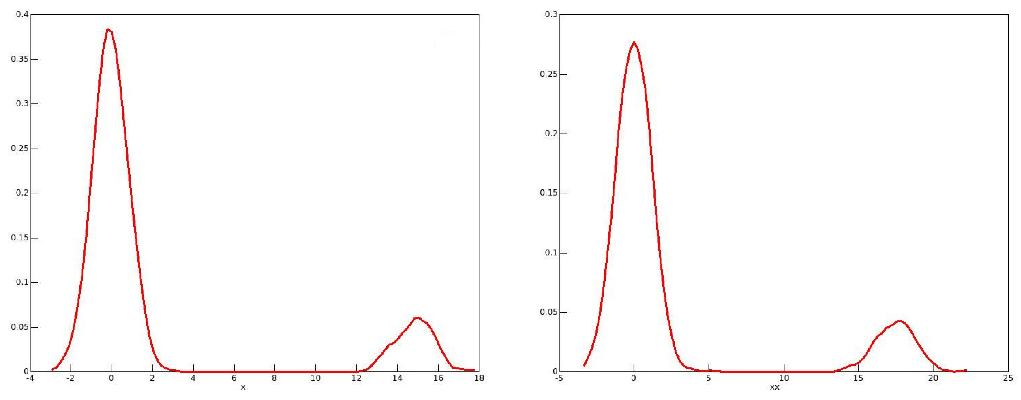
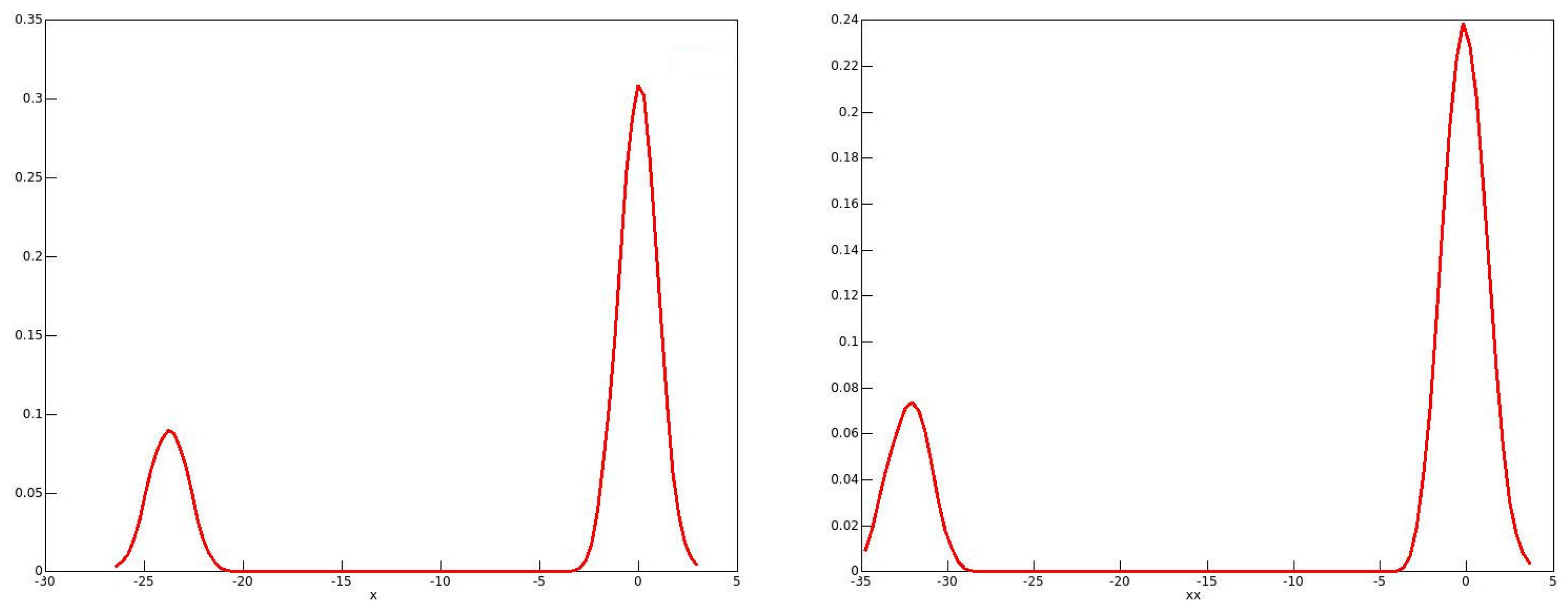
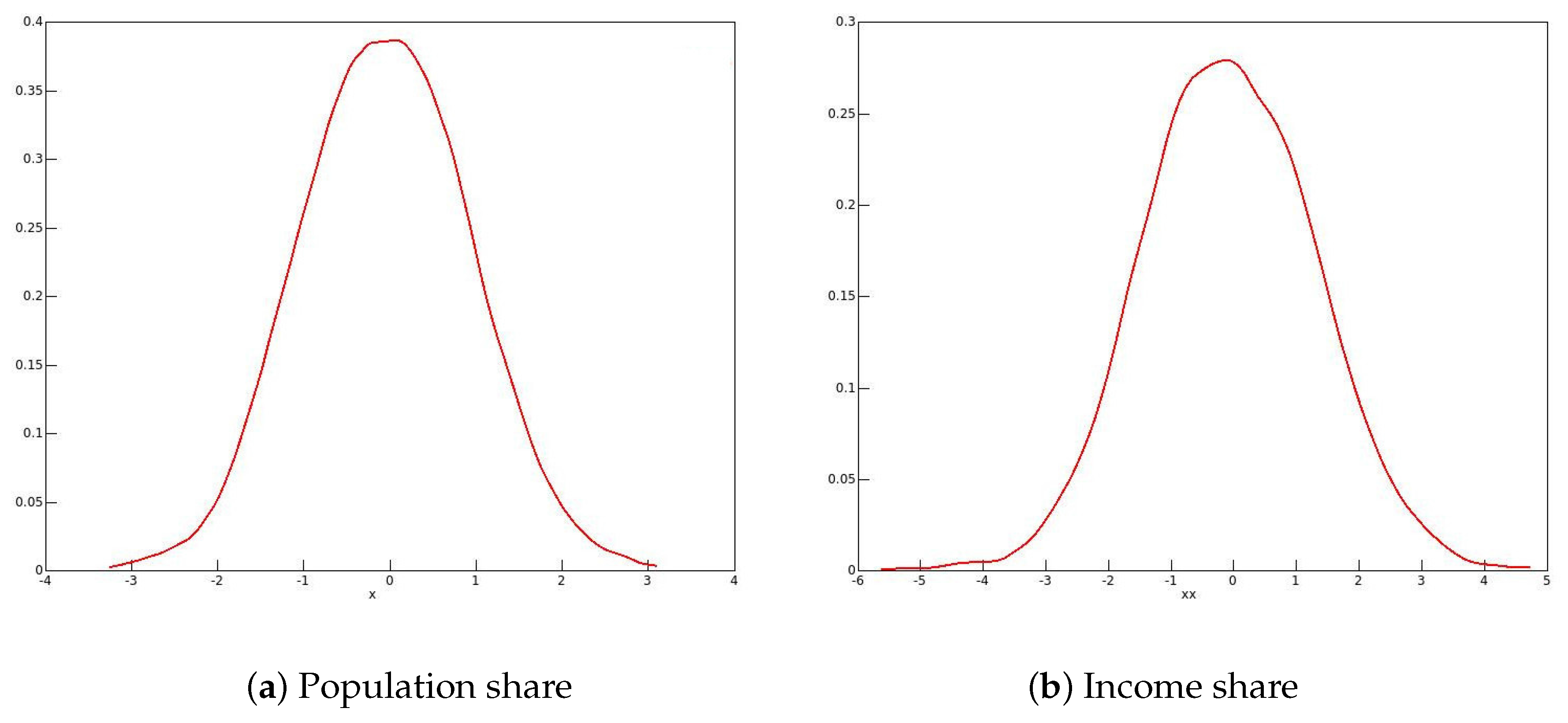
The reason for these phenomena with the 2001 and 2006 data emerges from looking at the distributions of the bootstrap statistics, of which kernel density plots in 2006 for males and for females are shown in Figure 1 and Figure 2 respectively.

One might expect the plots to resemble roughly a plot of the standard normal density. This would be the case if the long right-hand tail for men, and the long left-hand tail for women, each with a second mode, are neglected. It is well known that the resampling bootstrap can give highly misleading results with heavy-tailed data; see for instance Davidson (2012).

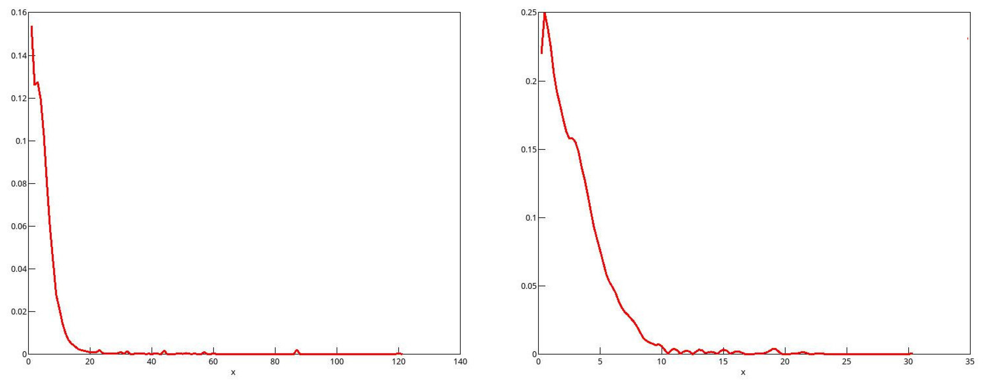
By looking at kernel density plots in Figure 3 of the sample income distributions for men and women in 2006, one can see evidence of the heavy right-hand tails for both sexes.

In addition, for all of the twenty-first century data, there is clear evidence of top-coding, since, in all cases, there are several observations equal to the largest income in the sample, while the next highest income is much lower. For instance, in the 2006 male sample, out of the 238,356 observations, there are 121 equal to the highest income of $1,202,480, while the next highest income in the sample is $872,522.

However, there is no reason to think that top-coding would have any effect on the estimated population shares, since their exact values do not matter. They do, of course, for the income shares, and so these are overestimated with top-coding. It turns out that the reason for the bimodal distributions of the bootstrap statistics is quite unrelated to top-coding. A closer look at the data for 2006 shows that a phenomenon that we may call “heaping” occurs in the data. What this means is that, for each recorded income, there are multiple instances, with comparatively large gaps between the distinct recorded incomes. While there is some measure of a similar heaping in the twentieth-century data, the phenomenon is much less marked. As an example, there is only one observation in the 1971 male data equal to the maximum value.

The consequences of this heaping are most salient with the 2006 data. For men, the median income is $35,000, and there are no fewer than 3228 observations of incomes apparently exactly equal to $35,000. The upper and lower limits for middle-class incomes that have been used in this study are $52,500 and $17,500, respectively. There are no observations of incomes equal to either of these limits, and this follows inevitably from the fact that all incomes no greater than $200,000 are recorded as exact integer multiples of $1000.

The data for women present a different picture, because the limits of $12,000 and $36,000 are integer multiples of $1000, and all incomes no greater than $100,000 are recorded as integer multiples of $1000. The maximum income of $310,136 is assigned to 99 observations; the median of $24,000 to 3316 observations; the lower limit of $12,000 to 4282 observations; and the upper limit of $36,000 to 2694 observations. The second highest recorded income is $306,763.

What this has meant for the bootstrap is that, of the 999 bootstrap repetitions with the data for men, all but 146 had a median of $35,000, the others having a median of $36,000. For the latter, the limits for middle-class income were $18,000 and $54,000, and including the 2052 observations of $54,000 in the numbers of the middle class greatly increases the population and income shares in those bootstrap samples relative to the shares of the 853 samples with a median of $35,000. At the other end, increasing the limit from $17,500 to $18,000 made no difference to the numbers, since there are no observations recorded in the interior of the range of the increase.

A similar analysis can be conducted with the data for women, but the reason for the bimodal distributions of the bootstrap statistics is clear: it arises on account of the data heaping. With the 2001 data, a bimodal distribution might have been expected, but all but five out of 999 bootstrap samples had a median equal to that of the original data, and, as expected, the distribution of the bootstrap statistics is unimodal in that case.

The data for years before 2001 have a much lesser amount of heaping and have unimodal bootstrap distributions. This no doubt implies that the bootstrap results are credible, although this conclusion is not of much worth since the bootstrap and asymptotic confidence intervals are nearly coincident.

3.3. Smoothing

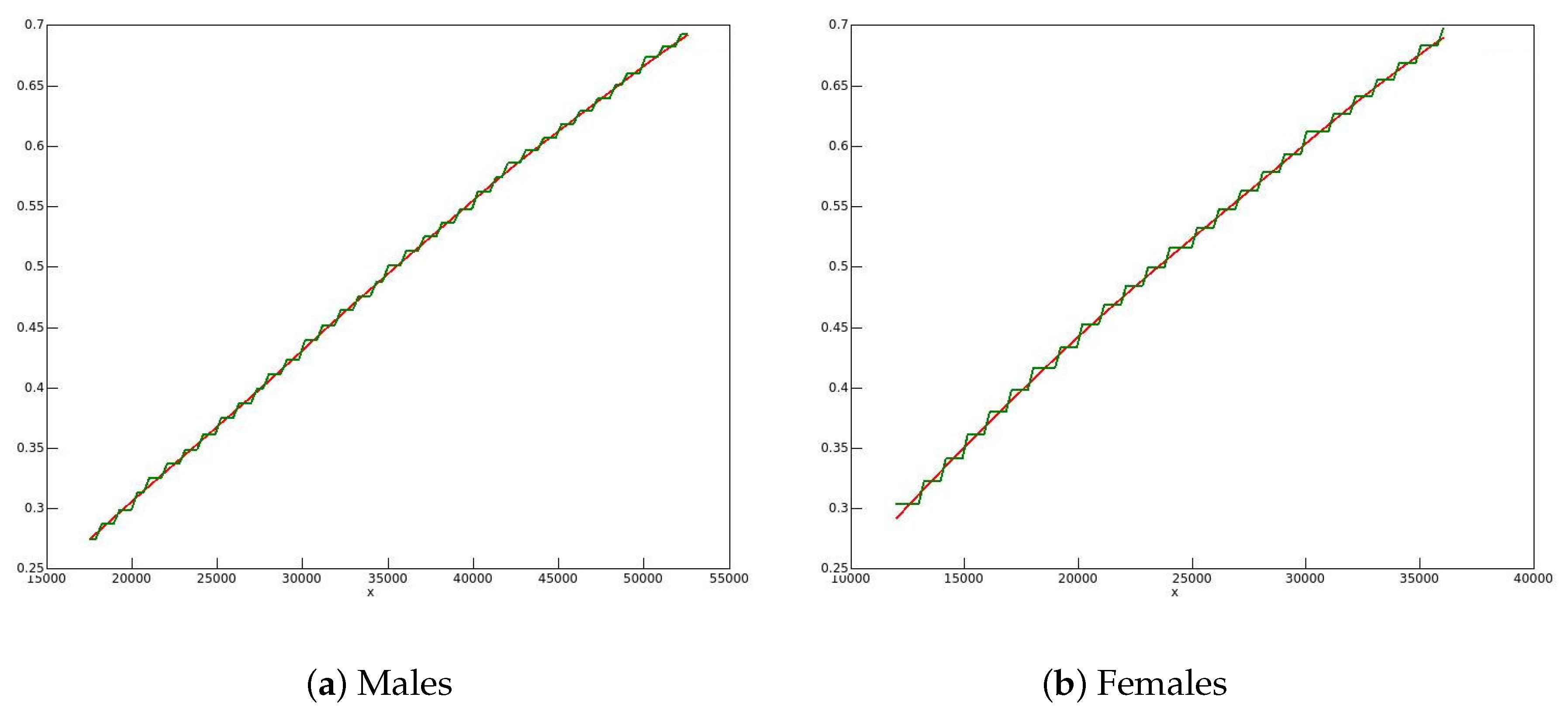
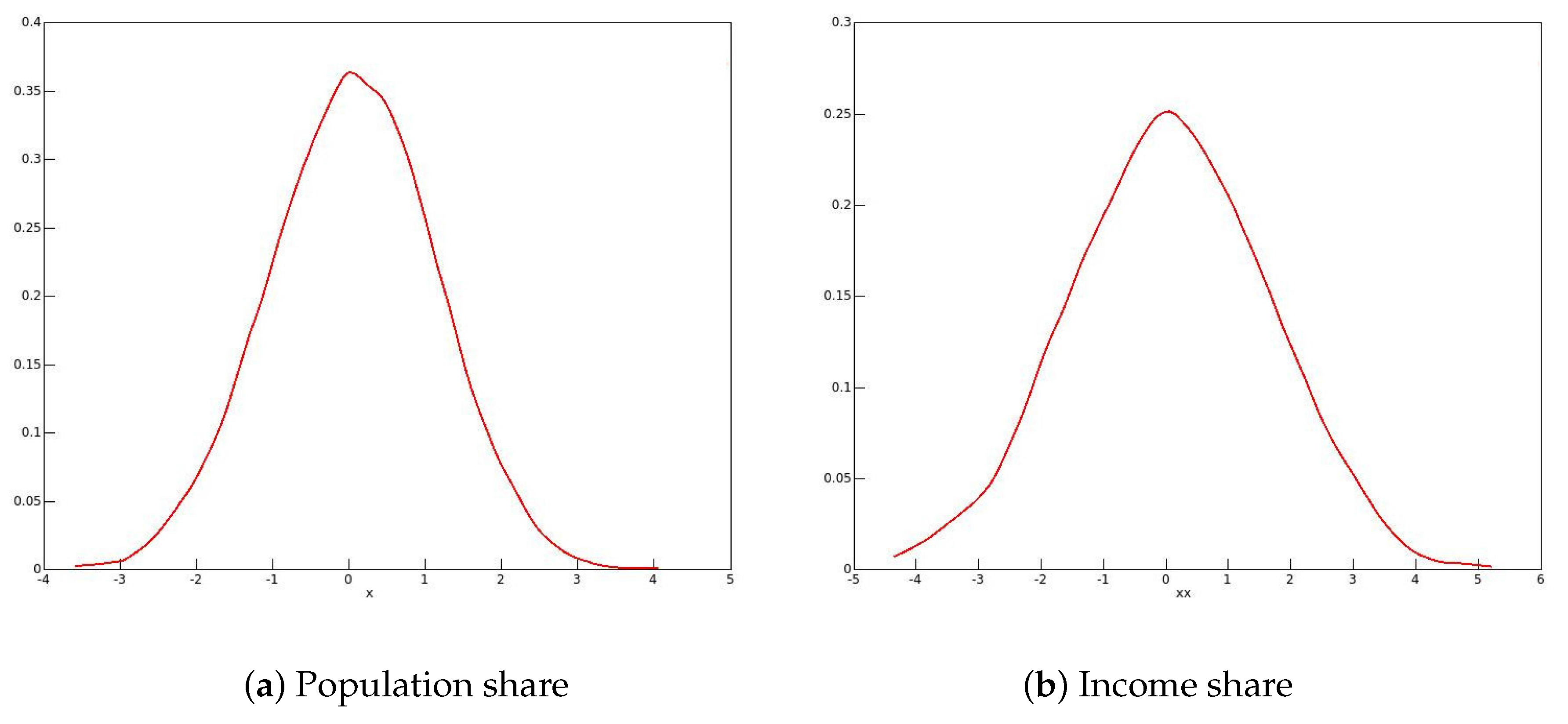
An obvious remedy for the heaping in the later datasets is to smooth them. The smoothed sample distribution may well be a better estimate of the population distribution than the heaped estimate, since the heaping is manifestly an artefact of the way in which the datasets were constructed. As always with smoothing, a troublesome question is the choice of bandwidth. Since the heaping occurs at integer multiples of $1000, the bandwidth h should be of a comparable magnitude in order to avoid an excessively discrete distribution. For $h=1000$, the raw EDFs of the 2006 data for men and women are plotted in Figure 4 along with the smoothed EDFs, for the range of incomes from half the median to 1.5 times the median. The heaped nature of the data for both sexes is quite evident in the green, unsmoothed, plots.

The (cumulative) kernel used for smoothing was the integrated Epanechnikov kernel. The smoothed estimate of the distribution is

$$F_{\mathrm{sm}}\left(y\right)=\frac{1}{N}\sum _{i=1}^{N}K\left(h^{-1}(y_i-y)\right),$$

(20)

where h is the bandwidth, and the cumulative kernel K is defined as

$$K\left(z\right)=\mathrm{I}\left(\left|z\right|\le \sqrt{5}\right)(\frac{3}{4\sqrt{5}}(z-z^3/15)+\frac{1}{2})+\mathrm{I}\left(z>\sqrt{5}\right).$$

(21)

where h is the bandwidth. Other choices of h greater than around 500 give qualitatively similar results.

For bootstrapping, resampling from the unsmoothed EDF is replaced by resampling from the smoothed EDF. Since the heaping phenomenon is banished by the smoothing, we can expect dramatically different results, in particular, a unimodal distribution of the bootstrap statistics. The CDF (20) describes a mixture distribution which assigns a weight of $1/N$ to the each of the distributions characterised by the terms in the sum. It is easily checked that K in (21) is a valid CDF, with support $[-\sqrt{5},\sqrt{5}]$. The term indexed by i in (20) has support $[y_i-h\sqrt{5},y_i+h\sqrt{5}]$.

To draw from the distribution (21), one starts from a uniform variate p from the U(0,1) distribution, and the draw is then $K^{-1}\left(p\right)$. The analytic form of $K^{-1}$ is not, I think, well known, and so I give it here for reference. It is2

$$K^{-1}\left(p\right)=2\sqrt{5}cos(\frac{1}{3}\left(2\pi -{cos}^{-1}(1-2p)\right)).$$

Thus, to draw from distribution (20), one may first draw the index i from the uniform distribution on $\{1,2,\dots ,N\}$, then draw p from U(0,1), and get the draw

$$y^{\ast }=y_i+h{K}^{-1}\left(p\right).$$

The effect is to resample from the unsmoothed distribution and then add some smoothing “noise” from the Epanechnikov distribution.

Although the smoothing preserves the mean of the distribution, it does not preserve the median, nor the population or income shares. If we accept the argument that the smoothed CDF is a better estimate of the true distribution than the unsmoothed one, then the smoothed median, and the shares in the smoothed distribution are also better estimators. In addition, the smoothed shares are the “true” values for the bootstrap DGP, and so the bootstrap statistics should test the hypothesis that they are true, not the hypothesis that the unsmoothed shares are true.

With the 2006 data for men, the new estimates of the shares are 0.421 for the population and 0.307 for income, slightly higher than the estimates from the raw data. The bootstrap confidence intervals are, for the population share, $[0.419,0.423]$ and, for the income share, $[0.305,0.310]$. They are of roughly the same width as the asymptotic intervals.

With the data for women, the new share estimates are 0.393 and 0.298, substantially lower than the unsmoothed estimates, and the confidence interval for the population share is $[0.390,0.395]$, and, for the income share $[0.295,0.301]$. Unsurprisingly, the smoothed share estimates are roughly in the middle of the respective intervals.

In Figure 5 (men) and Figure 6 (women), kernel density plots are shown for the distribution of the bootstrap statistics. There is no trace of bimodality, and so it seems that smoothing has indeed corrected the heaping problem.

3.4. Hypothesis Tests

In this section, the results of testing various hypotheses are found. All of the test statistics are asymptotic, as we have seen that when bootstrap inference differs greatly from asymptotic, the unsmoothed bootstrap, at least, is likely to be unreliable.

First are tests of hypotheses that the population and income shares for each sex did not change from one census until the next one. For instance, can one reject the hypothesis that the population share of the male middle class did not change from 1981 to 1991? Next are tests of hypotheses that the shares of men and women are the same in each census. For instance, can one reject the hypothesis that the income shares of men and women were the same in 2001?

The test results are expressed as asymptotic t statistics, rather than asymptotic p values, since in most cases the hypothesis is rejected strongly, and a p value very close to zero does not let one judge just how strong the rejection is. However, in some cases, the hypotheses are not rejected, and in some other cases, the sign of the statistic differs from the signs of the other statistics for the same sort of hypothesis.

For the first group of tests, the results of which are found in

Table 9. t statistics for hypothesis of no change in share between consecutive censuses.

Period	PS (Men)	PS (Women)	IS (Men)	IS (Women)
1971–1981	8.571726	2.299586	4.740735	6.571228
1981–1991	16.702812	0.311744	26.933620	6.875789
1991–2001	26.128047	−12.835861	53.350095	−7.954860
2001–2006	11.322294	−0.752581	43.943449	7.824492

, the sign of the statistic is positive if the decline in a share from the earlier to the later census is positive. A negative statistic indicates that the estimated share rose between the two censuses.

Remark 3.

All but two hypotheses of no change between two censuses are strongly rejected. The two exceptions concern the female population share, which did not change significantly either between 1981 and 1991 or between 2001 and 2006. There are two significantly positive increases, for the female population and income shares from 1991 to 2001.

In

Table 10. t statistics for hypothesis of equal shares for men and women.

Census	PS	IS
1971	32.526094	32.306558
1981	49.137099	60.112426
1991	50.265363	69.768414
2001	12.902812	20.345573
2006	7.824492	−12.143588

are found the statistics for testing the hypothesis that the share of men and women is the same for a given census. A positive statistic means that the estimated male share is greater than the female.

4. Conclusions

The main contribution of this paper is probably the theoretical part. The empirical results are not really surprising, although they do document clearly how the population and income shares of the male middle class have fallen over the period since 1970. In addition, one sees the results of the considerable increase in female labour market participation. Although the bootstrap has not shown itself especially useful for formal inference, the evolution over time of the distribution of the bootstrap statistics shows very clearly the increasing polarisation of Canadian society, with the growth of a heavy right-hand tail in the income distributions of both men and women.

The main obstacle to inference, whether asymptotic or bootstrap, with the twenty-first century data has been seen to be the problem of heaping, or excessively rounding, the data. The smoothing technique proposed here appears to lead to more reliable inference, but truly reliable inference would need better data.

References

- Atkinson, Anthony B. 1970. On the measurement of inequality. Journal of Economic Theory 2: 244–63. [Google Scholar] [CrossRef]
- Bahadur, R. Raj. 1966. A Note on Quantiles in Large Samples. Annals of Mathematical Statistics 37: 577–80. [Google Scholar] [CrossRef]
- Beach, Charles M. 2016. Changing income inequality: A distributional paradigm for Canada. Canadian Journal of Economics 49: 1229–92. [Google Scholar] [CrossRef]
- Blackorby, Charles, Walter Bossert, and David Donaldson. 1999. Income Inequality Measurement: The Normative Approach. In Handbook of Income Inequality Measurement. Edited by Jacques Silber. New York: Springer, pp. 133–62. [Google Scholar]
- Brzozowski, Matthew, Martin Gervais, Paul Klein, and Michio Suzuki. 2010. Consumption, income, and wealth inequality in Canada. Review of Economic Dynamics 13: 52–75. [Google Scholar] [CrossRef]
- Castells-Quintana, David, Raul Ramos, and Vicente Royuela. 2015. Income inequality in European Regions: Recent trends and determinants. Review of Regional Research 35: 123–46. [Google Scholar] [CrossRef] [Green Version]
- Cowell, Frank A. 1999. Estimation of Inequality Indices. In Handbook of Income Inequality Measurement. Edited by Jacques Silber. New York: Springer, pp. 269–90. [Google Scholar]
- Davidson, Russell. 2012. Statistical Inference in the Presence of Heavy Tails. Econometrics Journal 15: C31–C53. [Google Scholar] [CrossRef]
- Davidson, Russell, and Jean-Yves Duclos. 1997. Statistical Inference for Measurement of the Incidence of Taxes and Transfers. Econometrica 65: 1453–65. [Google Scholar] [CrossRef]
- Davidson, Russell, and Jean-Yves Duclos. 2000. Statistical Inference for Stochastic Dominance and for the Measurement of Poverty and Inequality. Econometrica 68: 1435–64. [Google Scholar] [CrossRef]
- Davidson, Russell, and James G. MacKinnon. 2006. Bootstrap Methods in Econometrics. In Palgrave Handbook of Econometrics. Edited by Terence C. Mills and Kerry Patterson. London: Palgrave-Macmillan, vol. 1, Econometric Theory. [Google Scholar]
- Davison, Anthony Christopher, and David Victor Hinkley. 1997. Bootstrap Methods and Their Application. Cambridge: Cambridge University Press. [Google Scholar]
- DiCiccio, Thomas J., and Bradley Efron. 1996. Bootstrap confidence intervals (with discussion). Statistical Science 11: 189–228. [Google Scholar]
- Foster, James E., and Michael C. Wolfson. 2010. Polarization and the decline of the middle class: Canada and the U.S. Journal of Economic Inequality 8: 247–73, Reprint of 1992 original article. [Google Scholar] [CrossRef]
- Hall, Peter. 1992. The Bootstrap and Edgeworth Expansion. New York: Springer-Verlag. [Google Scholar]
- Heathcote, Jonathan, Fabrizio Perri, and Giovanni L. Violante. 2010. Unequal we stand: An empirical analysis of economic inequality in the United States, 1967–2006. Review of Economic Dynamics 13: 15–51. [Google Scholar] [CrossRef]
- Kuznets, Simon. 1955. Economic Growth and Income Inequality. American Economic Review 45: 1–28. [Google Scholar]
- Ryu, Hang Keun. 2013. A bottom poor sensitive Gini coefficient and maximum entropy estimation of income distributions. Economics Letters 118: 370–74. [Google Scholar] [CrossRef]
- Wolff, Edward N. 2013. The Asset Price Meltdown, Rising Leverage, and the Wealth of the Middle Class. Journal of Economic Issues 47: 333–42. [Google Scholar] [CrossRef]
- Wolfson, Michael C. 1994. When Inequalities Diverge. American Economic Review 84: 353–58. [Google Scholar]