Data-Driven Jump Detection Thresholds for Application in Jump Regressions

1
Amazon.com, 399 Fairview Ave N, Seattle, WA 98109, USA
2
Department of Economics, Duke University, Durham, NC 27708, USA
*
Author to whom correspondence should be addressed.
Econometrics 2018, 6(2), 16; https://0-doi-org.brum.beds.ac.uk/10.3390/econometrics6020016
Submission received: 8 January 2018
/
Revised: 24 February 2018
/
Accepted: 24 February 2018
/
Published: 26 March 2018
Abstract
:This paper develops a method to select the threshold in threshold-based jump detection methods. The method is motivated by an analysis of threshold-based jump detection methods in the context of jump-diffusion models. We show that over the range of sampling frequencies a researcher is most likely to encounter that the usual in-fill asymptotics provide a poor guide for selecting the jump threshold. Because of this we develop a sample-based method. Our method estimates the number of jumps over a grid of thresholds and selects the optimal threshold at what we term the ‘take-off’ point in the estimated number of jumps. We show that this method consistently estimates the jumps and their indices as the sampling interval goes to zero. In several Monte Carlo studies we evaluate the performance of our method based on its ability to accurately locate jumps and its ability to distinguish between true jumps and large diffusive moves. In one of these Monte Carlo studies we evaluate the performance of our method in a jump regression context. Finally, we apply our method in two empirical studies. In one we estimate the number of jumps and report the jump threshold our method selects for three commonly used market indices. In the other empirical application we perform a series of jump regressions using our method to select the jump threshold.
Keywords:
efficient estimation; high-frequency data; jumps; semimartingale; specification test; stochastic volatilityJEL Classification:
C5; C52; G121. Introduction
Modeling asset prices with jumps has proven to be successful, both empirically and theoretically. Because of this a method to accurately and reliably estimate the timing and magnitude of jumps in asset pricing models would greatly aid the existing literature.
Since being introduced in Mancini (2001,2004) and threshold-based methods have become popular ways to estimate the jumps in time series data. The essential idea of these methods is that if an observed return is sufficiently large in absolute value then it is likely that the interval in which that return was taken contained a jump. To think about such an idea consider a standard jump-diffusion process for a log-asset price:
where is thought of as the drift of the process, is a time-varying volatility process, and is some finite activity jump process. (See Section 2 for a more rigorous definition of the jump-diffusion processes we consider in this paper.) Defining the returns of the observed process X as
where is the sampling interval, n is the number of high frequency increments per day, and for the asymptotic approximations. Note that is the geometric return in the asset price over the interval . Given a sequence of thresholds, , a threshold technique would label a return interval as containing a jump if . While Mancini (2001) originally set a common practice has emerged to use where and are parameters selected by the researcher and is the level of the local volatility around each return interval.1 Typically, values are or and is left as a tuning parameter.
If or the parameter has a convenient interpretation. Since the diffusive moves in are on the order using or we see that the tuning parameter has the interpretation of being essentially the number of local standard deviations of the process. A threshold-based jump selection scheme of this form then has the convenient interpretation of labeling returns as containing a jump (or multiple jumps) if the return is larger in absolute value than local standard deviations. While this provides a nice interpretation of the method, unfortunately the literature leaves the choice up to the researcher. The goal of the current paper is to provide a method for the selection of . (We leave or since what is important in practice is the relative size of a ‘typical’ increment and . See Jacod and Protter (2012, p. 248) for a discussion.)
Our primary focus in this paper is effective jump detection for the jump regression context of Li et al. (2017a) and Li et al. (2017b) where . We can think of such a setting as estimating in the following model
where are the return intervals in Z thought to contain a jump, where is the total number of identified jumps. In finance applications, Z is the log of a market index and Y is the log of a stock price. The underlying theoretical model is
where is the instantaneous jump operator (i.e., ), and the orthogonality condition that identifies is .2 Equation (3) is the empirical counterpart of (4). Li et al. (2017a) contains more explanation of the theoretical model and the identifying orthogonality condition.
With a truncation threshold of the form we would estimate as
Notice how crucially and thereby the estimated in (3) depends on the choice of . There are two types of jump classification errors that can be made: (i) incorrectly labeling a particular interval as containing a jump when it does not, and (ii) omitting an interval that actually contains a jump. If we set too low a threshold, we make type-(i) errors and include return intervals in that do not actually contain jumps, and that could potentially badly bias the estimated ‘jump beta’.
To see why we do not want to set too high a threshold and make a type-(ii) errors, we need to think about the variance of our estimated jump beta. To do so consider a heuristic model where at the jumps times we have
where the are independent and identically distributed with common variances . In addition, assume that the continuous returns are sufficiently small so that regardless of the truncation threshold used no continuous returns are included in the set of estimated jump returns. In this simplified setting
Notice that in this heuristic model that the variance of the estimated jump beta decreases as the number of jumps included in regression increases, i.e., as the set grows. If a truncation threshold of the form were used the variance of the estimator would be decreasing in .
Figure 1 illustrates these ideas using some empirical data. The left panel plots the jump beta for the jump regression of the SDPR S&P500 ETF (SPY) against the SDPR utilities ETF (XLU) for the years 2007 to 2014 using five-minute returns over a grid of jump threshold parameters. Notice that going down from to about that the hypothesis of a constant jump beta might be supported, i.e., that where are the true jump times in Z. The plotted jump beta is obviously noisy, but the estimated jump betas might very well be centered around a true and constant value. However after about the estimated jump betas for this asset begin to rapidly decline. It is not hard to imagine that after about the jump regressions became wildly corrupted by the addition of return intervals containing only diffusive moves. The right panel plots the reciprocal of the variance of the estimated jump betas along the same grid of jump threshold parameters as the reciprocal of the variance of an estimator is often thought of as a measure of the ‘precision’ of the estimator. Notice how the precision increases as decreases and we add return intervals to the jump regression. As in the left panel we plot a line at . If after around our jump regression begins to be rapidly corrupted by the addition of return intervals that only contain diffusive moves then, even though the precision of our estimator is increasing, our estimates of the jump beta are likely to be significantly biased. These panels illustrate the trade-off mentioned earlier in selecting a jump threshold. To decrease the variance of our estimated jump beta (or increase its precision) we would like a low jump threshold, but too low a jump threshold will likely bias our jump beta since we will likely include many returns that only contain diffusive moves.
In this paper, we develop a new method to balance the trade-off of setting too low a threshold and potentially including return intervals that only contain diffusive moves versus setting too high a threshold and potentially excluding return intervals that actually contain true jumps. The main idea is to find the value of for which the jump count function (defined below) ‘bends’ most sharply. Intuitively this could be thought of as the ‘take-off’ point of the jump count function. Selecting a threshold at this ‘take-off’ point should greatly reduce the number of misclassifications while maintaining many of the true jumps. We implement this idea by computing the point of maximum curvature to a smooth sieve-type estimator applied to the jump count function.
A related paper Figueroa-López and Nisen (2013) derives an optimal rate for the threshold in a threshold-based jump detection scheme with the goal of estimating the integrated variance. Using a loss function that equally penalizes jump misclassifications and missed jumps, Figueroa-López and Nisen (2013) find that the optimal threshold should be on the order of similar to the threshold originally proposed in Mancini (2001). Since is of order this result does not provide any guidance on the scale of the threshold to choose. Any threshold of the form for any would be just as optimal in their setting. This presents a major challenge for practitioners. Because of this Figueroa-López and Nisen (2013) provide an iterative method for selecting the scale of the truncation threshold. This iterative method however is not motivated by a theory of the jumps or the returns and adds an additional estimation step for any researcher hoping to use their method.
While we could have used truncation thresholds of the form for some in our paper and investigated the choice of the scale of the threshold, i.e., the choice of A we did not for two reasons. First, the difference in the relative convergence rates of and are tiny when or (see the discussion in Jacod and Protter (2012, p. 248)). Second, we feel using provides a convenient interpretation for the tuning parameter and therefore using is preferable.
The rest of the paper is organized as follows. Section 2 presents the setting. Our methodology and the main theory about its consistency are developed in Section 3 and Section 4. Section 5 and Section 6 present the results from a series of Monte Carlo studies and two empirical applications respectively. Finally, Section 7 provides a conclusion. All proofs are in the Appendix A.
2. The Setting
We start with introducing the formal setup for our analysis. The following notations are used throughout. We denote the transpose of a matrix A by . The adjoint matrix of a square matrix A is denoted . For two vectors a and b, we write if the inequality holds component-wise. The functions , and Tr denote matrix vectorization, determinant and trace, respectively. The Euclidean norm of a linear space is denoted . We use to denote the set of nonzero real numbers, that is, . The cardinality of a (possibly random) set is denoted . For any random variable , we use the standard shorthand notation satisfies some property} for { satisfies some property}. The largest smaller integer function is denoted by . For two sequences of positive real numbers and , we write if for some constant and all n. All limits are for . We use , and to denote convergence in probability, convergence in law, and stable convergence in law, respectively.
2.1. The Underlying Processes
The object of study of the paper is the optimal selecting of the cutoff level for a threshold-style jump detection scheme. Let X be the process under consideration and, for simplicity of exposition, assume that X is one-dimensional. (The results can be trivially generalized to settings where X is multidimensional, but doing so would unnecessarily burden the notation.)
We proceed with the formal setup. Let X be defined on a filtered probability space represented as . Throughout the paper, all processes are assumed to be càdlàg adapted. Our basic assumption is that X is an Itô semimartingale (see, e.g., Jacod and Protter 2012, sct 2.1.4) with the form
where the drift takes value in ; the volatility process takes value in , the set of positive real numbers; W is a standard Brownian motion; is a predictable function; is a Poisson random measure on with its compensator for some measure on . The jump of X at time t is denoted by , where . Finally, the spot volatility of X at time t is denoted by . Our basic regularity condition for X is given by the following assumption.
Assumption 1.
(a) The process b is locally bounded; (b) is nonsingular for ; (c) .
The only nontrivial restriction in Assumption 1 is the assumption of finite activity jumps in X. This assumption is used mainly for simplicity as our focus in the paper are ‘big’ jumps, i.e., jumps that are not ‘sufficiently’ close to zero. Alternatively, we can drop Assumption 1(c) and focus on jumps with sizes bounded away from zero.3
Turning to the sampling scheme, we assume that X is observed at discrete times , for , within the fixed time interval . Following standard notation as discussed in the Introduction, the increments of X are denoted by Below, we consider an infill asymptotic setting, that is, as .
3. Limits
Here we present some initial results needed to develop the data-drive method described in Section 4. To do so we first discuss how to think about inference for the jumps; next, we introduce the jump count function, and then we proceed to discuss jump misclassifications.
3.1. Inference for the Jump Marks
As was discussed in the introduction, in order to disentangle jumps from the diffusive component of asset returns, we choose a sequence of truncation threshold values which satisfy the following condition:
In order to analyze the jumps of the process X it is helpful to introduce some notation. First, define to be the successive jump times of the process X. Next, define two random sets and which collect respectively the indices of the jumps times in the interval and the jump times themselves. Since the jumps in X are assumed to be of finite activity, these two sets are almost surely finite as well. For the jump in X that occurs at time , we call its mark. Finally, define a Borel measurable subset as a (temporal-spatial) region. We do so in order to think about restricting our observation set to only those jumps that fall within a given region. To do so define the set .
With these definitions we can think about the true and estimated sets that index the jumps in a given sample. For each , we denote by the unique random index i such that . We set
The set-valued statistic collects the indices of returns whose ‘marks’ are in the region , where the truncation criterion eliminates diffusive returns asymptotically. The set collects the indices of sampling intervals that contain the jumps with marks in . Clearly, the set is random and unobservable. We also impose the following mild regularity condition on , which amounts to requiring that the jump marks of X almost surely do not fall on the boundary of .
Assumption 2.
, where denotes the boundary of .
Under Assumptions 1 and 2 it can be shown that for a fixed that consistently estimates the jumps, i.e., . (See, for example, Li et al. 2017a.) The goal of the current paper is to make dependent on the sample and the sampling frequency.
3.2. The Jump Count Function
The now-standard method to define the truncation level is
where is an estimate of the general level of local volatility, typical settings are or , and is a tuning parameter. Since the diffusive moves in X are on the order and is just under , the tuning parameter has the convenient interpretation of essentially being the number of local standard deviations. This definition of motivates a definition of the sample index of the jumps that depends on the truncation threshold . With this in mind define
By the presumed finite activity of the jump process in X there are only a (random) finite number of jumps and we wish to identify the set .
In order to do so it proves convenient to define the jump count function
Evidently, is non-increasing, piecewise flat with discontinuities at the order statistics of . Notice decreases to zero as . For each fixed (and for any ), it can be shown that for a large enough n, i.e., for a small enough that
since and converges to . (See (Li et al. 2017a) for the details and a more thorough discussion.)
3.3. Jump Misclassifications
We think of a jump selection procedure as having a ‘misclassification’ if, for some return interval , we yet over the region we have . That is, if we label the return interval as containing a jump when no true jump occurred.
In order to think about jump misclassifications consider the jump count function solely for the diffusive moves. Defining the continuous moves of the process as for and we can define the jump count function of the continuous moves as
For a given jump threshold and sampling frequency , the function counts the diffusive moves that are ‘incorrectly’ labeled as jumps. Since the diffusive moves are locally Gaussian we see that is simply a Bernoulli random variables with probability of success equal to where and is the cumulative distribution function of the standard normal density. This is because
where Z is a standard normal random variable. Because of this is simply a binomial random variable with the same probability and n draws. This implies
For a fixed it is fairly straight forward to show that as , which implies in the limit that the number of misclassifications goes to zero. This result however turns out not to be a good guide for the range of sampling frequencies most often encountered in practice. Table 1 reports the expected number of yearly misclassification, i.e., with , using for over a range of threshold parameter values. The range of sampling frequencies corresponds to ten minute, five minute, one minute, and one second sampling in a typical trading day. Notice that for each selected threshold that the number of expected misclassifications is always increasing in the table.4 This is in stark contrast to what one might expect given the asymptotic theory. Since the timing and magnitude of the jumps do not vary with the sampling frequency and the diffusive moves vanish as shrinks to zero one might be led to conclude that the truncation thresholds could be decreased as the sampling frequency increases. The result in Table 1 shows that for the range of frequencies a researcher is most likely to encounter that this is not the case. Because of this result, while we remain alert to the asymptotic theory, we seek to find an optimal threshold parameter that is sample driven, not one based solely on the asymptotic theory.
4. The Curvature Method
As briefly discussed above in the introduction, the selection of a jump threshold, i.e., the selection of in Equation (11), involves a trade off between setting too high a threshold and failing to include all of the jumps against setting too low a threshold and erroneously labeling diffusive moves as jumps. For example, setting would correctly identify every jump but would also include every diffusive move. Similarly, setting would guarantee that no diffusive moves were incorrectly labeled as jumps, but would fail to identify any of the jumps.
We can use the results of Section 3 to guide the selection of a suitable . Under the modeling assumptions of Section 2, there are a finite (but random) number of jumps on the interval . From the theory (Jacod and Protter 2012; Li et al. 2017a) we know that for any fixed the truncation scheme correctly classifies all jumps when n is sufficiently large. Thus, for any fixed the jump count Function (13) satisfies almost surely. Furthermore, for a fixed n and for higher values of we should expect the jump count function to have a long flat region that is level at about , but we should also expect the jump count function to rise sharply at lower values of where many diffusive moves start getting erroneously classified as jumps. So the task is to determine from the jump count function that value of where the jump count function starts to increase sharply as declines. We think of this point as the point at which the jump count function begins to ‘take-off’. Our solution to find this ‘take-off’ point is to look for the value of at which the jump count function ‘kinks’ or ‘bends’ most sharply.
The way to mathematically define a ‘kink’ or sharpest ‘bend’ in a smooth function is the point of maximum curvature. The curvature of a smooth function is defined as
Intuitively, if we think of the function f as lying in a two-dimensional plane and representing the direction of travel of some object, the curvature of f represents the rate at which the direction of travel is changing. (Or more rigorously the magnitude of the rate of change of the unit tangent vector to the curve.) The point of maximum curvature then is the point at which the direction of travel changes the most.
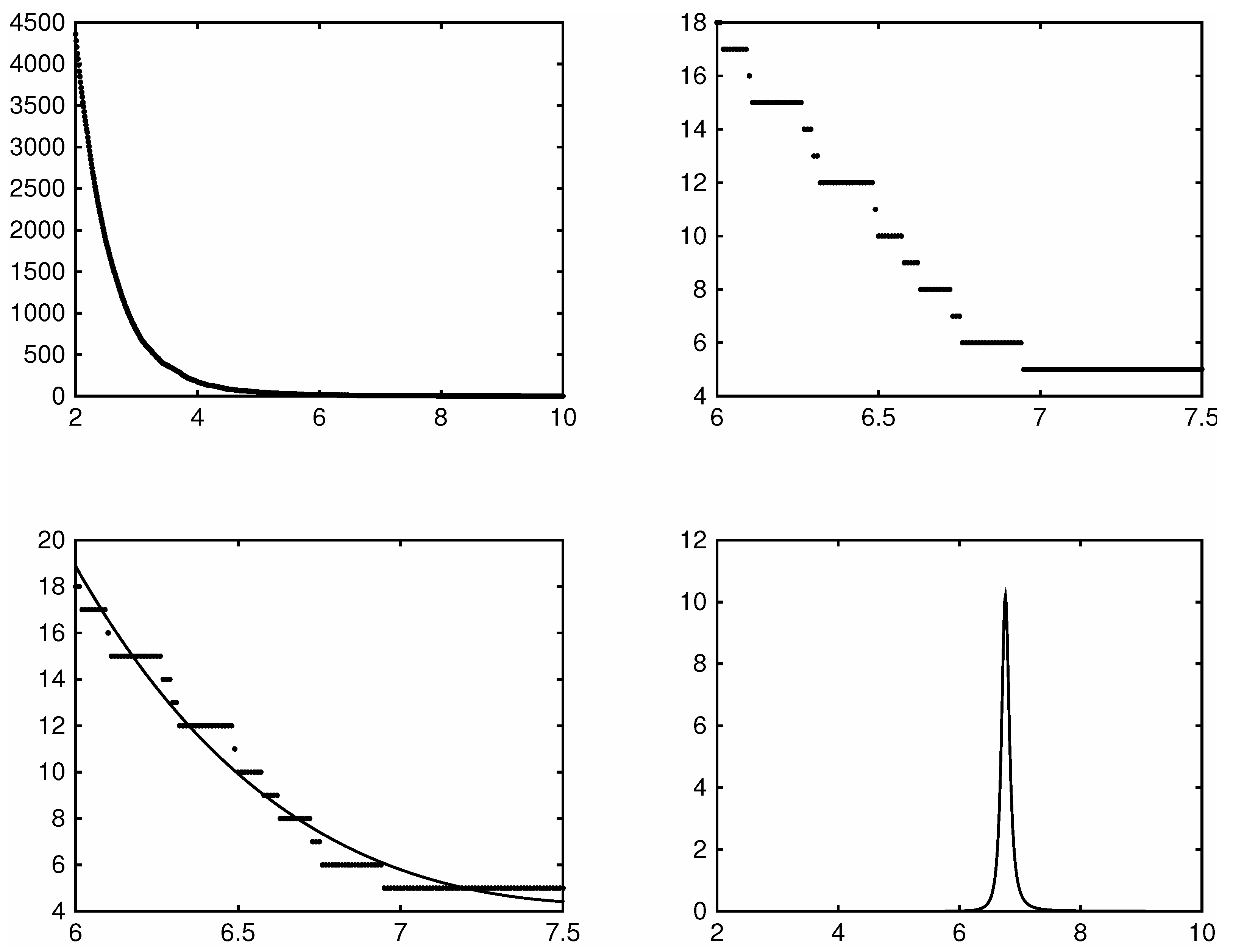
However, being piece-wise flat, the raw jump count function itself is ill-suited for this purpose, as evident in the top two panels of Figure 2. These panels plot the jump count function for the five minute returns of the SDPR S&P500 ETF during the year 2014. In the top left panel the domain is too wide making the steps barely noticeable. Zooming in however on the domain the top right panel clearly shows the jump count function to be piece-wise flat.
Given this problem, we work with a smoother sieve estimator fitted to the jump count function. A natural choice might seem to be kernels or splines but these turn out to be ineffective due to the small wiggles and discontinuities that these functions have in their higher order derivatives. These wiggles and discontinuities in turn significantly affect the curvature of these functions making the point of maximum curvature often more dependent on the particular choice of which kernels or splines was chosen rather than the data. A far better approach is to do a least-squares projection of the observed jump count function onto a set of smooth basis functions. Given the shape of the jump count function, we use basis functions
where we need for the point of maximum curvature to be well-defined. Using these basis functions we can define the projection of the jump count function onto as
In practice we find that these basis functions result in projections with extremely tight5 fits that have very high s for low values of or . Because of this the projection itself amounts to a compact numerical representation of approximately the same information as in the raw jump count function itself.
With this idea in mind we select as the value that maximizes the curvature of the appropriately smoothed jump count function, i.e.,
where . We refer to such a selection method in what follows as the ‘curvature method’.
Setting the threshold right at this point of maximum curvature or ‘kink’ point then allows for a great many of the true jumps to be located, but guards against overly misclassify diffusive moves. Because of this, the procedure is evidently very conservative in that it lets through only a small number of diffusive moves. However, in a jump regression setting a very conservative jump selection procedure is to be preferred as the loss from including diffusive moves is very high because doing so potentially biases the estimates whereas incorrectly missing a true jump only entails a small loss of efficiency.
Though conservative, the curvature method is asymptotically accurate. We show this in Theorem 1 below. The theorem shows that in the limit the curvature method correctly identifies all of the jumps and excludes any returns that contain only diffusive moves. The theorem relies on the following definition for the convergence of random vectors with possibly different length: for a sequence of random integers and a sequence of random elements, we write if we have both and
Theorem 1.
Under Assumptions 1 and 2 and with we have that
- (a)
- , and
- (b)
- .
The theorem above shows that as that the jump count function using our procedure will converge in probability to the true number of jumps and that the estimated index of the jumps over a region will converge in probability to the true index over that region.
5. Monte Carlo Studies
We evaluate the performance of our threshold selection method on simulated data in three Monte Carlo studies. The first study compares our method with a method that simply chooses a fixed value of the truncation parameter . The second study evaluates how our method does at recovering jumps of varying magnitudes. Finally, the third study shows the performance of our method in a jump regression setting.
5.1. Comparing Our Method with Choosing a Fixed Truncation Constant
In the first Monte Carlo study we evaluate the performance of our threshold selection method against a method that simply chooses a fixed value of . (Where recall we label a return interval as containing a jump if .) The sample span is one year, containing trading days. Each day we simulate data using high-frequency returns to match what would correspond to one second sampling and consider return intervals of one second, one minute, five minutes, and ten minutes. There are 1000 Monte Carlo replications and we set .
The data generating process in this Monte Carlo study follows the model below. The model is taken from Li et al. (2017b) and accommodates features such as the leverage effect, price-volatility co-jumps, and heteroskedasticity in jump sizes. Let W and B be independent Brownian motions. We generate prices according to
The first displayed equation shows the price dynamics: X is the log asset price, V the local diffusive variance, is parameter that captures correlation between the continuous parts of X and V (the leverage effect), is a mean-zero Gaussian price jump, and is a Poisson counting process with intensity . The second displayed equation shows the variance dynamics: is the drift in V, is the log-variance jump, which occurs at the same time as price jumps and is exponential with parameter . The parameters calibrated (realistically) are given by
The negative value for the variance drift is needed to offset the positive upward drift generated by variance jumps with positive mean, and thereby keep from increasing off to infinity.
In addition to the selected threshold , we report two statistics for the Monte Carlo study. The first we term the jump ‘recovery rate’. This is the number of correctly identified jumps divided by the number of true jumps. A recovery rate of means every true jump was correctly identified whereas a recovery rate of means no true jumps were identified. The second statistic we term the ‘accuracy’ of the jump detection procedure. This is the number of correctly matched jumps divided by the number of estimated jumps. An accuracy of means that every return interval we estimated to include a jump actually contained a true jump whereas an accuracy of means that none of the return intervals we estimated to include a jump actually contained a true jump. Table 2 below reports the results of the first Monte Carlo study. All the statistics in the table are averages across the 1000 Monte Carlo replications. First notice that while the average selected value of decreases from ten minute sampling down to one second sampling. Such a result is to be hoped for since over the sampling range of ten minutes to one second the number of jump misclassifications, as was shown in Section 3.3, is actually increasing at higher sampling frequencies. A method that attempted to minimize jump misclassifications would ideally increase the jump threshold over this range to guard against such misclassifications. Our method appears to make some effort to do so.
Notice that the average recovery rates of the curvature procedure are generally as good as and sometimes better (rarely worse) than those using a fixed . At the same time, the average accuracy of the procedure is above for all sampling frequencies, unlike the fixed case. The curvature method can achieve substantially increased recovery rates with little sacrifice in accuracy. As for the other values of , the accuracy remains high but at the expense of a lower recovery rate than that of the curvature method.
5.2. Recovering Jumps of Varying Magnitudes
For the second Monte Carlo study, we use modification of a standard setup to examine how our method performed in recovering jumps of differing magnitudes. To this end we simulated jumps that, with equal probability, took sizes varying from one to ten unit standard deviations of the local volatility.6 To do this, we modeled the jumps as following a compound Poisson process, that once scaled for the local volatility, had a jump size density that followed a discrete uniform distribution taking values in the range . Using such a jump density allows us to observe how well our method can and cannot detect jumps of various magnitudes.
Letting be a vector of Brownian motions with , the model is defined as
where is an i.i.d. discrete uniform distribution that takes values in . (Setting allows for a dependence between and , i.e., a leverage effect.) We set so there should be on average a one-twelfth chance of a jump occurring each day. This is consistent with previous studies on market jumps. The data generating process for the diffusive moves and the volatility process is similar and based on that found in Li et al. (2017a).
We perform the study using 1000 replications and set , which corresponds to three years’ worth of simulated data. We use an Euler scheme to simulate the high-frequency data doing an initial simulation with which corresponds to sampling once every tenth of a second. We then sample these high-frequency returns at one second, one minute, five minute, and ten minute frequencies.
Table 3 reports the results of this Monte Carlo study. The table lists the averages across all 1000 Monte Carlo replications. Consistent with a theory of vanishing diffusive moves the recovery rates increase significantly with each increase in the sampling frequency. At a 10 minute frequency we recovery most jumps greater than eight local standard deviations, a few jumps between five and seven local standard deviations, and virtually no jumps of sizes one to four local standard deviations. Sampling at a five minute frequency we make significant gains in recovering jumps of five to seven local standard deviations. At a one minute sampling frequency we can uncover nearly all jumps except those of one local standard deviation. Finally, at one second sampling all of the jumps are recovered. (Note though that the increase in the sampling frequency going from one minute to one second sampling is significantly greater than going from ten to five to one minute sampling so the stark contrast between the one minute and the one second sampling should not be exaggerated.)
The average selected threshold parameter appears to decrease somewhat from ten minute to five minute to one minute sampling, but increases quite significantly going from one minute to one second sampling. Following the discussion in Section 3.3 the large increase in the selected threshold from one minute to one second sampling is to be hoped for as the number of expected jump misclassifications increases greatly going from one minute to one second sampling. The slight decrease in the average selected threshold parameter going from ten minute to one minute sampling, while not ideal in terms of the arguments of Section 3.3, does not appear to drastically change the accuracy of the estimated jumps. The accuracy over these three sampling frequencies is always above and only decreases to at one second sampling.
5.3. Jump Regression Setting
The third Monte Carlo study examines how our procedure performs in a jump regression context. A thorough overview of jump regressions can be found in Li et al. (2017a). Below we only give a brief overview of jump regressions and the results we use in our Monte Carlo study. Given two series of returns (often a proxy for the market) and (often the return on an asset price) a jump regression considers a regression of on only over the return intervals in which Z is thought to contain a jump. The null in many jump regression settings is that the jump regression coefficient, termed the jump beta, is constant at every jump time, i.e.,
For this Monte Carlo study we perform a test of a constant jump beta under both a simulated model that has a constant jump beta and a model with a time varying jump beta. We report rejection rates for the test as well as the average selected thresholds and the accuracy and recovery rates of the estimated jumps. For the test of a constant jump beta we use a bootstrap version of the determinant test of Li et al. (2017a).
We simulate data using a model adapted from Li et al. (2017a). The model takes the form
where W, , and B are three independent Brownian motions. and are compound Poisson jump processes where the jump size densities follow double-exponential (or Laplacian) distributions and the jump intensities are and respectively. We set .
The jump beta process follows the following specifications under the null and the alternative
where is a Brownian motion independent of W, , and B. The unconditional mean of under the alternative is 1. The model differs from Li et al. (2017a) only in the specification of different jump and diffusive betas.
We perform the study using 1000 replications and set , which corresponds to three years’ worth of simulated data. We use an Euler scheme to simulate the high-frequency data doing an initial simulation with which corresponds to sampling once every tenth of a second. We then sample these high-frequency returns at one second, one minute, five minute, and ten minute frequencies. These parameters were chosen to match the Monte Carlo study in Li et al. (2017a) as closely as possible.
Table 4 below reports the results of our study. Notice how differently the size of the test is affected by the choice of the jump threshold parameter. Using the curvature method the test is only moderately over-sized at ten and five minute sampling and not terribly over-sized at one minute sampling. (This is perhaps to be somewhat expected as Li et al. (2017a) found the test of a constant jump beta to be moderately over-sized.) These fairly mild over rejections using the curvature method however are in stark contrast to using a fixed . Notice that using a fixed how the size of the tests becomes progressively worse and worse as the sampling frequency increases. Even at ten and five minute sampling the test is quite over-sized. This result is due to the inclusion of return intervals in the jump regression that only contained diffusive moves thereby biasing the estimated jump beta. To see this notice that using the accuracy of the jump detection procedure deteriorates significantly as the sampling frequency increases. At one minute sampling the average accuracy is and at one second sampling the average accuracy is a very low . This means that in the respective jump regressions on average fully and of the respectively estimated returns did not actually contain a jump. In contrast using the curvature method the accuracy of the estimated jumps remains high at all sampling frequencies. Finally, note that the power of the test using both methods is consistent with the results in Li et al. (2017a).
6. Empirical Application
We considered two empirical applications. The first estimates the jumps and reports the jump threshold selected by our method for three commonly used and high liquid market indices. The second application reports the results of jump regressions of the nine SDPR sector ETFs against the SDPR S&P500 ETF using our method to select the jump threshold.
6.1. Estimating Jumps in Market Indices
For the E-mini S&P500 index futures (ES), the SPDR S&P500 ETF (SPY), and the VIX futures (VIX) we use the tools developed in this study to estimate the optimal jump thresholds for each series over a range of dates and a range of sampling frequencies. We report both the jump threshold selected by our method as well as the estimated number of jumps at each selected jump threshold. The SPY and ES series span the dates 3 January 2007 to 12 December 2014. The VIX series spans the dates 2 July 2012 to 30 April 2015. Only the more recent VIX futures data are used because Bollen and Whaley (2015) provide evidence that the VIX futures market was highly illiquidity and immature in prior periods. For each series we remove market holidays and partial trading days; and, to guard against possible adverse microstructure effects, we discard the first five minutes and the last five minutes of each trading day.
For each series we performed the estimation over both the entire sample and each complete calendar year within each sample. In addition, we performed the estimation using one minute, five minute, and ten minute intraday returns. Table 5 and Table 6 report the selected jump threshold and the estimated number of jumps at the selected jump threshold.
In Table 6 which reports the selected jump threshold , notice that for the E-mini S&P500 index futures (ES) and the SPDR S&P500 ETF (SPY) there appears to be somewhat of an increase in the selected threshold as the sampling frequency increases from ten minute to five minute to one minute sampling. As was discussed in Section 3.3 this is to be hoped for as the number of jump misclassifications is actually increasing over this range of sampling frequencies. For the VIX futures (VIX) we do not see much of a pattern in the selected jump threshold . This however should not be seen as evidence against our threshold selection procedure since Andersen et al. (2015) provide evidence that the high-frequency returns of the VIX futures might be well modeled as following an -stable distribution with . If this were true then not only would we not expect the same misclassification dynamics as in the diffusive case, but the correct scaling of the returns would be on the order of rather than .
For Table 5, which reports the estimated number of jumps, notice that the number of estimated jumps is always increasing as the sampling frequency increases. Note also that the number of jumps detected at the 5-min and 10-min frequencies is very small, reflecting the inherent conservative nature of the curvature method. In practice, common sense suggests that at these coarser frequencies the practitioner might elect to experiment a bit with slightly lower values of than those produced directly by the curvature method, which does define a sensible baseline however.
6.2. Jump Regressions
Using the nine SDPR sector ETFs we perform a series of jump regressions of the sector ETFs against the SDPR S&P500 market ETF (SPY). We determine the jumps in the SPY series via the jump threshold parameter based on the curvature method developed Section 4 above. Then to examine how sensitive these jump regressions are to different jump thresholds we consider two other thresholds and which are equal to plus and minus respectively. The reason for basing the jump threshold on the SPY series is that a jump regression only considers the beta for the regression of the specific asset return on the market return for intervals in which the market (SPY) is thought to have jumped. Note that the data are for the year 2009 and that we use one-minute returns to estimate the jumps but five-minute returns to perform the jump regressions.7 We chose the year 2009 because it was a representative year and one for which there appeared empirical support for a constant jump beta for each asset over the year.8
Table 7 reports the jump beta, the standard error of the jump beta, the of the regression, and the p-value of the null of a constant jump beta over the year. The p-values are calculated using a bootstrap version of the determinant test in Li et al. (2017a). The standard errors are calculated under a simplifying assumption that the volatility process of the diffusive moves is continuous across the market jump times; otherwise, inference becomes far more complicated but the conclusions barely changed in the end. For some of the portfolios the estimated beta seen in the table seems relatively insensitive to the 15% perturbations to , but there are some notable exceptions. In particular, the jump beta for the XLF (Finance) portfolio is quite lower ( vs. ) using versus . The same is also true but to a lesser degree for XLK (Technology), XLU (Utilities), and XLV (Health Care). These four are economically important portfolios where the beta value matters, and one does not want a misleading estimate obtained by letting in too many diffusive moves and thereby throwing off the jump regression. At the same time, note that for all nine portfolios the estimation precision obtained with is higher (lower standard error) than with , which reflects of course the inclusion of the more jumps, i.e., data points.
7. Conclusions
This paper introduced a method for selecting the threshold in threshold-based jump detection schemes. Previously the selection of the threshold in such schemes has been left to each researcher in each project to choose. This creates a problem because the number of estimated jumps in a series of observed returns can vary substantially depending on which threshold a researcher selects. Our method therefore advances the existing literature on asset price jumps because it provides a method for the selection of the jump threshold. Even further, we believe researchers will find our method intuitive and easy to implement in practice.
In developing our method, we first showed that over the range of sampling frequencies a researcher is most likely to encounter that the standard in-fill asymptotics provide a poor guide for the selection of the jump threshold. Because of this we developed a sample-based method. Our method is developed as follows. Given a series of observed returns, our method relies on first estimating the number of jumps in this series over a grid of possible thresholds. Doing so results in a jump count function where the value of the function is the number of estimated jumps in the series of returns at each value of the threshold in the grid. Our method then selects the chosen threshold as the threshold for which the curvature of a suitably smoothed version of the jump count function is maximized. We think of this point as being the point were the estimated number of jumps begins to ‘take-off’. We argue that selecting the threshold at this point should include many of the true jumps in the process and should guard against overly including returns that only contain diffusive moves. As the sampling size of the returns goes to zero we show that such a methodology will consistently estimate the jumps of a jump-diffusion model and asymptotically will exclude returns that only contain diffusive moves.
Having developed a methodology for selecting the threshold in threshold-based jump detection schemes we show its performance in several Monte Carlo studies and an empirical application. The Monte Carlo studies showed our method was able to recovery many of the true jumps in the data generating processes considered and maintained a high degree of accuracy in the returns it labeled as containing jumps. Further, one Monte Carlo study showed the improvement our method gave in a jump regression context. Finally, in two empirical studies we applied the method discussed to real world data. In the first empirical study we estimated the number jumps and provided the jump threshold selected by our method over a range of dates and sampling frequencies for three commonly used series in finance: the SPDR S&P500 ETF, the S&P500 E-mini futures, and the VIX futures. In the second empirical study we performed a series of jump regressions where we regressed the return intervals thought to contain jumps in the SDPR S&P500 ETF (SPY) on the corresponding return intervals in the SDPR sector ETFs using our method to select the jump times.
Acknowledgments
We would like to thank Tim Bollerslev, Jia Li, Andrew Patton, Dacheng Xiu and the entire financial econometrics lunch group at Duke for helpful discussions.
Author Contributions
Both authors contributed equally to the paper.
Conflicts of Interest
The authors declare no conflict of interest.
Appendix A. Proofs
To notational brevity below we refer to the optimally selected jump threshold as , that is , rather than as in the main text. For two positive sequences of real numbers and we use the following set of notations below: we write if as , we write if for some there exists such that for all we have , we write if for some there exists such that for all we have , and finally we write if for some there exists and such that for all we have .
We also drop the dependence of and on the region and simply write and instead.
Proof of Theorem 1.
(a) Since the jumps of X have finite activity, we can assume without any loss of generality that each interval contains at most one jump. (If not we can restrict the focus to the w.p.a.1 set of the sample paths upon which this condition holds.) We denote the continuous part of X by
Following Li, Todorov, and Tauchen (2014) notice that can be broken into two disjoint sets and defined as
The proof proceeds by showing
- (i)
- , and
- (ii)
- .
Part (i):
Recall that with . By Lemma A1 below we have . This implies as (or equivalently as ) since . Following Li, Todorov, and Tauchen (2014), we notice that implies that for any and an sufficiently large that we will have . These results imply
Next notice that
To see this notice that, almost surely,
Therefore w.p.a.1 the sets and will coincide.
Part (ii):
We first show a result concerning the distribution of the diffusive moves. Notice that because the diffusive moves are locally Gaussian that for a fixed that we have where and is the cumulative distribution function of the standard normal density.
Recalling that with notice that
Consider . Since is non-random we know and therefore . Next, we will use the result that for any where is the standard normal density. Using this result and the fact that for any we see
where the convergence above follows since at a faster rate than . This shows . ☐
(b) By part (a), it suffices to show that
Observe that is simply . We deduce the desired convergence by the same arguments as in part (a).
Lemma A1.
For with and as defined in Section 3.3, we have that at rate .
Proof.
Recall that . Where is the curvature of a function and where is the projection of onto the set of basis functions .
Since the approximation of onto the set of basis functions is found by a least squares projection of onto g we can solve for analytically. To do so define so that where is the inner product on the space of real-valued functions on the domain . Defining we can express the vector of coefficients
which implies each coefficient
Recall from the proof of Theorem 1 that for a fixed . Since the jump process in X is assumed to be of finite activity and increases without bound as we can see that . (Note the limit here is for holding n fixed.) This result implies that in a neighborhood around that since . (Where the limit is now for holding fixed in a neighborhood around .) We can use this result to derive an expression for each when is small and n is large.9
For some algebra shows
where the function is the incomplete Gamma function. (When or similar expressions can be deduced.) We proceed by examining each component of (A11) in the limit in order to derive a bound on in the limit. For any fixed we can express as
where and . (DLMF, Section 8.11(i)) If we think of in (A12) we see . This implies that for in (A11) and therefore that
for in (A11). The error function can be written as (DLMF, Section 7.12)
which shows . This implies that
as well for in (A11). Combing these results we see
for . Using a similar derivation as in (A11) and the arguments above it can be shown that both and as well. Recall since for all we see .
Having provided rates for how the coefficients of go to zero we will use these results to describe the behavior of the the curvature function of in the limit as well. Doing so will allow us to think about how will behave in the limit. The curvature10 of is
Since notice that
and
We showed above that for that each coefficient
which implies that both
and
Looking at the denominator of in (A17) we see that
and therefore that for an n sufficiently large that since at a faster rate than . To see this, note that
Note as well that since and at slower rate than that and therefore .
Having concluded that and we can think about how might behave in the limit as well. Recall that with . Fixing an and thinking about the function on the domain notice that for any that since is a monotonically decreasing function of . Since and for all we see that as well.
Having shown that we will find its rate. First, however, we need to establish a result concerning linear functions. Note that for any non-zero linear function the rate at which when for a constant will be the same as the rate that because we express for some and . With this in mind define the function and consider its Taylor approximation around when is ‘small’. That is
Since as , for a sufficiently large n, we will have . Since we took the approximation around and assumed was ‘small’ we see that the Taylor approximation error in (A25) will also be negligible compared to . This shows that in a sufficiently small neighborhood around when is ‘small’ that will be approximately linear in and therefore the rate that will be the same as the rate that . Since the rate that is given by the rate that . We showed earlier that this implies that and since we see at rate . This implies finally that at rate . ☐
Appendix B. NOTES
The entire interval comprises intervals of width . Let are denote indexes (labels) of the intervals that actually contain Z jumps. Note that the labels in vary with n but the cardinality does not vary with n since that is the actual (finite) number of jumps.
We need to characterize the asymptotic behavior of the increments in the Y and Z processes across both the non-jump and jump intervals. For the diffusive (non-jump) intervals, we have from Jacod and Protter (2012)
where are local volatilities, and are conditionally correlated Gaussian random variables with unit variance each. For the intervals that actually Z jumps we have from LTT
where are the jump times, the actual jumps, is the (constant) jump beta, and are "mixed-normal" random variables with a relatively simple but non-stand distribution defined by the diffusive variation in Y and Z across the jump interval.
As per the main text, let denote the intervals labeled as jumps by the jump detection scheme, where we suppress the dependence on for now. If then all jumps are perfectly detected, and we are in the setup of LTT, which has been covered. The following is interesting only if , i.e., there are diffusive intervals erroneously miss-classified as jump intervals.
Suppose across the entire jump interval
which implicitly assumes equal beta at jump intervals and by construction is a continuous process.
Suppose we incorrectly include extra diffusive terms into the regression. From Jacod and Protter (2012) we have that
In what follows it matters how grows (if at all) with n. Thus we write
The most interesting and relevant case is when , but considering the cases provide further insights.
The jump regression estimator is
Suppose B is positive and finite. Then
The above is just the mean of random variables, where the r for the is drawn from whatever probability density governs the (incorrect) inclusion of the diffusive terms in ; hence,
where . Note that the support of could be a strict subset of , and that will put zero mass points at the jump times . By similar reasoning we have that
Using familiar jump regression arguments we have that
Putting everything together we have that asymptotically (A31) acts as
where is the now classical “realized beta” for diffusive regression, and
References
- Andersen, Torben G., Oleg Bondarenko, Viktor Todorov, and George Tauchen. 2015. The fine structure of equity-index option dynamics. Journal of Econometrics 187: 532–46. [Google Scholar] [CrossRef]
- Bollen, Nicolas P. B., and Robert F. Whaley. 2015. On the Supply of and Demand for Volatility. Working paper, Nashville, USA: Vanderbilt University. [Google Scholar]
- Figueroa-López, José E., and Jeffrey Nisen. 2013. Optimally thresholded realized power variations for Lévy jump diffusion models. Stochastic Processes and their Applications 123: 2648–77. [Google Scholar] [CrossRef]
- Jacod, Jean, and Philip E. Protter. 2012. Discretization of Processes. Berlin: Springer. [Google Scholar]
- Li, Jia, Viktor Todorov, and George Tauchen. 2017a. Jump Regressions. Econometrica 85: 173–95. [Google Scholar] [CrossRef]
- Li, Jia, Viktor Todorov, and George Tauchen. 2017b. Robust Jump Regressions. Journal of the American Statistical Association 112: 332–41. [Google Scholar] [CrossRef]
- Mancini, Cecilia. 2001. Disentangling the Jumps of the Diffusion in a Geometric Jumping Brownian Motion. Giornale dell’Istituto Italiano degli Attuari LXIV: 19–47. [Google Scholar]
- Mancini, Cecilia. 2004. Estimation of the characteristics of the jumps of a general Poisson-diffusion model. Scandinavian Actuarial Journal 1: 42–52. [Google Scholar] [CrossRef]
| 1 | In discussions on estimating asset pricing jumps, the volatility is typically treated as being known and locally constant. In practice it needs to be estimated. |
| 2 | In the financial econometrics literature, the symbol is used three different ways: is the sampling interval; is the first difference operator over the interval of width , and means the instantaneous jump in X at time t. Note that if X is continuous at t. |
| 3 | Yet another strategy, that can allow for studying dependence in infinite activity jumps, is to use higher order powers in the statistics that we develop henceforth. This, however, comes at the price of losing some efficiency for the analysis of the ‘big’ jumps. |
| 4 | The intuition behind the result in Table 1 is that when we have for resulting in actually increasing as decreases (or n increases). |
| 5 | The projection minimizes with respect to . |
| 6 | Where to preserve the jump sizes across sampling frequencies we used the local volatility in terms of return intervals at the coarsest sampling frequency, which here corresponded to sampling at a ten minute frequency. |
| 7 | The SPY asset is sufficiently liquid to use to identify jump intervals at the 1-min level; the subsequent aggregation to 5-min returns is a correction for possible trading friction noise in the returns of the less liquid sector-specific assets. |
| 8 | Not all years showed such evidence of constant jump betas. For the sake of exposition we do not report the results from these years since there is not as much to learn from examining the jump regression results using different jump thresholds if the jump beta is time-varying. Results for all years are available on request, however. |
| 9 | We limit our scope to the case when is small because we are primarily interested in limiting the number of misclassifications that might occur in the jump count function and, as was shown in Section 3.2, these increase exponentially as . |
| 10 | The equation in (A17) is actually for the signed curvature. However the basis functions used here always have a positive signed curvature so that the curvature and the signed curvature coincide. |
Figure 1.
A jump regression illustration of the importance of the threshold parameter. NOTE: Along the horizontal axes is the jump threshold parameter . The left panel plots the jump beta for the jump regression of the SDPR S&P500 ETF (SPY) on the utilities sector ETF (XLU) across a grid of threshold parameters used to estimate the jumps in SPY. The right panel plots the inverse variance of the estimated jump betas in these regressions. A vertical line has been plotted in both panels at where it appears the estimated jump beta begins to rapidly decrease. The estimates for these plots are based on five minute return data for both series spanning the years 2007 to 2014.
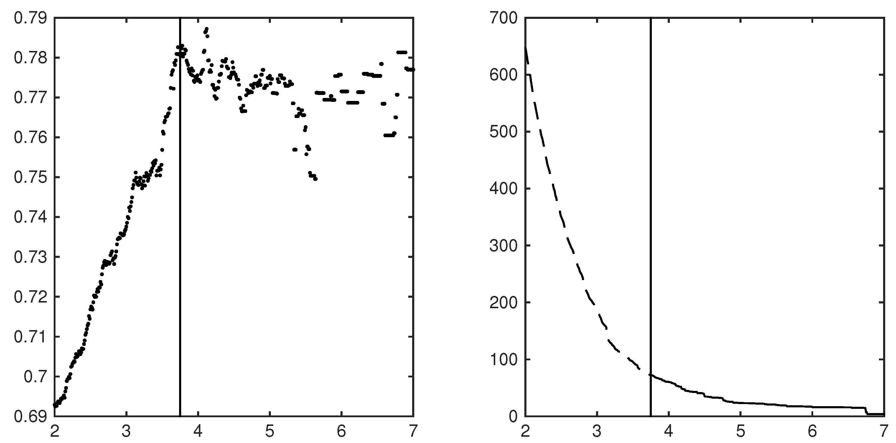
Figure 2.
An illustration of the jump threshold selection method. NOTE: Along the horizontal axes is the jump threshold parameter . The top left panel plots the estimated number of jumps over a grid of . The top right zooms in and plots the estimated number of jumps over . The bottom left panel adds a plot of the fitted basis function. The bottom right plots the curvature of the fitted basis function. The estimates for these plots are based on five minute return data from the SDPR S&P500 ETF (SPY) spanning the year 2014. We set . See Section 3.3 and Section 4 for details on the estimated number of jumps and the fitted basis functions.


Table 1.
Expected Number of Yearly Jump Misclassifications.
| Threshold Parameter | ||||||||
|---|---|---|---|---|---|---|---|---|
| Freq. | ||||||||
| 39 | 2.78 | 0.328 | 0.030 | 0.0021 | 0.0001 | 4.8 × 10⁻⁶ | 1.5 × 10⁻⁷ | 3.8 × 10⁻⁹ |
| 78 | 5.04 | 0.578 | 0.051 | 0.0035 | 0.0002 | 7.2 × 10⁻⁶ | 2.2 × 10⁻⁷ | 5.2 × 10⁻⁹ |
| 390 | 19.96 | 2.140 | 0.175 | 0.0109 | 0.0005 | 1.9 × 10⁻⁵ | 5.1 × 10⁻⁷ | 1.1 × 10⁻⁸ |
| 390 × 60 | 640.63 | 57.304 | 3.822 | 0.1897 | 0.0070 | 0.0002 | 3.9 × 10⁻⁶ | 5.8 × 10⁻⁸ |
NOTE: Table reports the expected number of yearly () diffusive returns that would be misclassified as jumps for each fixed using the result that where is the jump count function of the diffusive moves. We set .
Table 2.
Comparison against a fixed truncation scheme: Monte Carlo averages (%).
| Curvature | Fixed Truncated Parameter | ||||||||||
|---|---|---|---|---|---|---|---|---|---|---|---|
| Method | |||||||||||
| Freq. | REC | ACC | REC | ACC | REC | ACC | REC | ACC | REC | ACC | |
| 10 min | 4.83 | 29.35 | 98.61 | 39.22 | 89.36 | 27.75 | 99.63 | 17.17 | 100.00 | 11.08 | 100.00 |
| 5 min | 4.65 | 49.49 | 98.95 | 56.09 | 92.63 | 46.21 | 99.91 | 36.83 | 100.00 | 28.65 | 100.00 |
| 1 min | 4.22 | 79.61 | 94.85 | 80.71 | 87.09 | 76.08 | 99.90 | 71.42 | 100.00 | 65.89 | 100.00 |
| 1 s | 5.95 | 96.70 | 91.48 | 97.46 | 25.74 | 97.03 | 98.95 | 96.54 | 100.00 | 95.73 | 100.00 |
NOTE: REC is average jump recovery rate, ACC is the average accuracy of estimated jumps, and is the average selected threshold parameter across the Monte Carlo replications. The jump recovery rate is defined as the number of correctly matched jumps divided by the number of true jumps. The jump accuracy is defined as the number of correctly matched jumps divided by the number of estimated jumps. The jump accuracy and recovery rate are in percentage terms. The results are based on 1000 replications following the data generating process outlined in (22) and (23).
Table 3.
Recovering jumps of varying magnitudes: Monte Carlo averages.
| Recovery Rates (%) by Jump Size | ||||||||||||
|---|---|---|---|---|---|---|---|---|---|---|---|---|
| Freq. | Accuracy (%) | |||||||||||
| 10 min | 5.27 | 99.71 | 0.32 | 0.15 | 1.27 | 5.51 | 18.53 | 41.48 | 65.93 | 83.83 | 94.07 | 97.79 |
| 5 min | 5.07 | 99.83 | 0.31 | 0.91 | 11.68 | 46.62 | 84.69 | 97.67 | 99.86 | 99.96 | 99.94 | 99.97 |
| 1 min | 4.41 | 98.22 | 6.38 | 93.90 | 99.99 | 100.00 | 99.95 | 99.97 | 99.99 | 100.00 | 99.98 | 100.00 |
| 1 s | 5.72 | 94.28 | 100.00 | 100.00 | 100.00 | 100.00 | 100.00 | 100.00 | 100.00 | 100.00 | 100.00 | 100.00 |
NOTE: The recovery rates are for jumps of sizes equal to 1–10 unit local standard deviations in terms of return intervals sampled at a ten minute frequency. The above indicates a unit of local standard deviation. The average selected threshold parameter across Monte Carlo replications is denoted . The jump recovery rate is defined as the number of correctly matched jumps divided by the number of true jumps. The jump accuracy is defined as the number of correctly matched jumps divided by the number of estimated jumps. The results are based on 1000 replications following the data generating process outlined in Section 5.2.
Table 4.
Monte Carlo rejection rates (%) for tests of a constant jump beta.
| Curvature Method | ||||||||||||
|---|---|---|---|---|---|---|---|---|---|---|---|---|
| Under | Under | |||||||||||
| Average | Nominal Level | Average | Nominal Level | |||||||||
| Freq. | ACC | REC | 10% | 5% | 1% | ACC | REC | 10% | 5% | 1% | ||
| 10 min | 5.64 | 99.8 | 34.4 | 11.6 | 6.5 | 1.8 | 5.65 | 99.8 | 34.6 | 52.1 | 42.6 | 22.8 |
| 5 min | 4.42 | 99.7 | 52.4 | 10.6 | 5.8 | 1.8 | 4.42 | 99.8 | 52.9 | 71.0 | 62.0 | 45.4 |
| 1 min | 5.04 | 98.1 | 78.6 | 13.5 | 8.3 | 2.2 | 5.01 | 98.1 | 78.6 | 98.6 | 96.9 | 94.1 |
| 1 s | 5.57 | 92.6 | 96.0 | 19.7 | 11.6 | 4.1 | 5.59 | 92.7 | 96.1 | 100.0 | 100.0 | 100.0 |
| Fixed α = 4 as in Li et al. (2017a) | ||||||||||||
| Under | Under | |||||||||||
| Average | Nominal Level | Average | Nominal Level | |||||||||
| Freq. | ACC | REC | 10% | 5% | 1% | ACC | REC | 10% | 5% | 1% | ||
| 10 min | 4.00 | 92.8 | 48.3 | 12.7 | 7.1 | 3.0 | 4.00 | 92.9 | 48.6 | 52.0 | 41.4 | 23.1 |
| 5 min | 4.00 | 93.6 | 61.0 | 12.7 | 7.5 | 2.6 | 4.00 | 93.7 | 61.0 | 70.9 | 61.5 | 43.1 |
| 1 min | 4.00 | 88.1 | 80.5 | 18.8 | 10.5 | 4.2 | 4.00 | 88.2 | 80.6 | 98.7 | 96.9 | 94.5 |
| 1 s | 4.00 | 26.5 | 97.2 | 99.1 | 96.6 | 86.5 | 4.00 | 26.3 | 97.3 | 100.0 | 100.0 | 100.0 |
NOTE: The rejection rates are for the null of a constant jump beta using a bootstrap version of the determinant test of Li et al. (2017a). REC is average jump recovery rate, ACC is the average accuracy of estimated jumps, and a is the average selected threshold parameter a across the Monte Carlo replications. The jump recovery rate is defined as the number of correctly matched jumps divided by the number of true jumps. The jump accuracy is defined as the number of correctly matched jumps divided by the number of estimated jumps. The jump accuracy and recovery rate are in percentage terms. The results are based on 1000 replications following the data generating processes for the null and alternative as outlined in Section 5.3.
Table 5.
Estimated Number of Jumps.
| SPDR S&P500 ETF (SPY) | |||||||||
|---|---|---|---|---|---|---|---|---|---|
| Frequency | Full Sample | 2007 | 2008 | 2009 | 2010 | 2011 | 2012 | 2013 | 2014 |
| 10 min | 6 | 3 | 1 | 1 | 0 | 0 | 0 | 0 | 1 |
| 5 min | 20 | 3 | 4 | 1 | 3 | 1 | 5 | 3 | 1 |
| 1 min | 81 | 6 | 13 | 13 | 10 | 10 | 12 | 5 | 6 |
| E-mini S&P500 Futures (ES) | |||||||||
| Frequency | Full Sample | 2007 | 2008 | 2009 | 2010 | 2011 | 2012 | 2013 | 2014 |
| 10 min | 6 | 1 | 0 | 1 | 0 | 0 | 1 | 0 | 1 |
| 5 min | 20 | 2 | 3 | 2 | 3 | 1 | 4 | 3 | 1 |
| 1 min | 100 | 12 | 9 | 9 | 13 | 14 | 14 | 11 | 12 |
| VIX Futures | |||||||||
| Frequency | Full Sample | 2013 | 2014 | ||||||
| 10 min | 3 | 2 | 1 | ||||||
| 5 min | 9 | 6 | 2 | ||||||
| 1 min | 43 | 17 | 11 | ||||||
NOTE: The table reports the estimated number of jumps for each sample at the chosen jump threshold given in Table 6. The frequency refers to the sampling frequency of the returns. The SPY and ES series span the dates 3 January 2007 to 12 December 2014. The VIX series spans the dates 2 July 2012 to 30 April 2015.
Table 6.
Selected Jump Threshold ().
| SPDR S&P500 ETF (SPY) | |||||||||
|---|---|---|---|---|---|---|---|---|---|
| Frequency | Full Sample | 2007 | 2008 | 2009 | 2010 | 2011 | 2012 | 2013 | 2014 |
| 10 min | 5.61 | 5.81 | 5.20 | 5.25 | 6.07 | 5.38 | 6.13 | 5.26 | 5.71 |
| 5 min | 6.13 | 5.98 | 5.54 | 5.81 | 6.30 | 5.80 | 6.60 | 6.17 | 7.01 |
| 1 min | 6.67 | 7.12 | 6.13 | 6.24 | 6.49 | 6.43 | 7.59 | 6.79 | 6.76 |
| E-mini S&P500 Futures (ES) | |||||||||
| Frequency | Full Sample | 2007 | 2008 | 2009 | 2010 | 2011 | 2012 | 2013 | 2014 |
| 10 min | 5.60 | 5.97 | 5.25 | 5.39 | 5.81 | 5.37 | 6.06 | 5.24 | 5.52 |
| 5 min | 6.15 | 6.20 | 5.66 | 5.86 | 6.26 | 5.90 | 6.52 | 6.04 | 6.72 |
| 1 min | 6.11 | 6.45 | 6.08 | 5.94 | 5.80 | 5.95 | 6.69 | 5.93 | 6.13 |
| VIX Futures | |||||||||
| Frequency | Full Sample | 2013 | 2014 | ||||||
| 10 min | 5.78 | 5.65 | 5.67 | ||||||
| 5 min | 5.52 | 5.38 | 5.41 | ||||||
| 1 min | 5.49 | 5.18 | 5.30 | ||||||
NOTE: The table reports the selected jump threshold for each sample based on the procedure in Section 4. The frequency refers to the sampling frequency of the returns. The SPY and ES series span the dates 3 January 2007 to 12 December 2014. The VIX series spans the dates 2 July 2012 to 30 April 2015.
Table 7.
Jump regression results for the nine SDPR sector ETFs against the SDPR S&P500 ETF.
| Jump Thresholds | |||||
|---|---|---|---|---|---|
| Asset | S.E. | -Value | |||
| XLB | 1.049 | 0.060 | 0.894 | 0.021 | |
| 0.996 | 0.102 | 0.905 | 0.045 | ||
| 0.988 | 0.112 | 0.922 | 0.015 | ||
| XLE | 0.948 | 0.065 | 0.877 | 0.029 | |
| 0.902 | 0.101 | 0.984 | 0.679 | ||
| 0.934 | 0.117 | 0.994 | 0.471 | ||
| XLF | 1.182 | 0.144 | 0.866 | 0.360 | |
| 1.687 | 0.577 | 0.984 | 0.956 | ||
| 1.691 | 0.661 | 0.998 | 0.872 | ||
| XLI | 1.046 | 0.048 | 0.955 | 0.151 | |
| 0.967 | 0.078 | 0.991 | 0.648 | ||
| 0.973 | 0.086 | 0.994 | 0.271 | ||
| XLK | 0.697 | 0.057 | 0.916 | 0.196 | |
| 0.711 | 0.105 | 0.922 | 0.086 | ||
| 0.741 | 0.114 | 0.988 | 0.350 | ||
| XLP | 0.684 | 0.059 | 0.908 | 0.363 | |
| 0.712 | 0.133 | 0.935 | 0.275 | ||
| 0.754 | 0.146 | 0.962 | 0.173 | ||
| XLU | 0.890 | 0.079 | 0.865 | 0.118 | |
| 1.127 | 0.128 | 0.914 | 0.183 | ||
| 1.192 | 0.135 | 0.974 | 0.073 | ||
| XLV | 0.764 | 0.060 | 0.905 | 0.339 | |
| 0.885 | 0.102 | 0.903 | 0.071 | ||
| 0.973 | 0.105 | 0.999 | 0.819 | ||
| XLY | 0.956 | 0.049 | 0.932 | 0.023 | |
| 1.032 | 0.073 | 0.955 | 0.073 | ||
| 0.998 | 0.077 | 0.962 | 0.018 | ||
NOTE: This table reports the results from jump regression of the listed asset against the SDPR S&P500 ETF (SPY). The data are returns on the nine SDPR sector ETFs for the year 2009. The selected jump threshold parameters are based on the estimated jumps in the SPY returns series as this is the left-hand side variable in the jump regressions. The jumps were located using one-minute returns and the jump regressions where performed using five-minute returns. The threshold is the estimated threshold using the curvature method and and are plus and minus respectively. The standard errors are calculated under the simplifying assumption that the volatility is continuous over the day. The p-values are from a bootstrap version of the determinant test in Li et al. (2017a).
© 2018 by the authors. Licensee MDPI, Basel, Switzerland. This article is an open access article distributed under the terms and conditions of the Creative Commons Attribution (CC BY) license (http://creativecommons.org/licenses/by/4.0/).
Share and Cite
MDPI and ACS Style
Davies, R.; Tauchen, G. Data-Driven Jump Detection Thresholds for Application in Jump Regressions. Econometrics 2018, 6, 16. https://0-doi-org.brum.beds.ac.uk/10.3390/econometrics6020016
AMA Style
Davies R, Tauchen G. Data-Driven Jump Detection Thresholds for Application in Jump Regressions. Econometrics. 2018; 6(2):16. https://0-doi-org.brum.beds.ac.uk/10.3390/econometrics6020016
Chicago/Turabian StyleDavies, Robert, and George Tauchen. 2018. "Data-Driven Jump Detection Thresholds for Application in Jump Regressions" Econometrics 6, no. 2: 16. https://0-doi-org.brum.beds.ac.uk/10.3390/econometrics6020016
Note that from the first issue of 2016, this journal uses article numbers instead of page numbers. See further details here.