Decomposing the Bonferroni Inequality Index by Subgroups: Shapley Value and Balance of Inequality

1
Department of Statistical Sciences, “Sapienza” University of Rome, Piazzale Aldo Moro 5, Rome 00185, Italy
2
Italian National Institute of Statistics—ISTAT, Via Cesare Balbo 16, Rome 00184, Italy
*
Author to whom correspondence should be addressed.
Econometrics 2018, 6(2), 18; https://0-doi-org.brum.beds.ac.uk/10.3390/econometrics6020018
Submission received: 11 December 2017
/
Revised: 20 March 2018
/
Accepted: 23 March 2018
/
Published: 2 April 2018
(This article belongs to the Special Issue Econometrics and Income Inequality)
Abstract
:Additive decomposability is an interesting feature of inequality indices which, however, is not always fulfilled; solutions to overcome such an issue have been given by Deutsch and Silber (2007) and by Di Maio and Landoni (2017). In this paper, we apply these methods, based on the “Shapley value” and the “balance of inequality” respectively, to the Bonferroni inequality index. We also discuss a comparison with the Gini concentration index and highlight interesting properties of the Bonferroni index.
Keywords:
inequality measurement; Bonferroni index; Gini concentration ratio; decomposition methods; Shapley value; balance of inequality; complex survey dataJEL Classification:
D63; C71; I321. Introduction
Carlo Emilio Bonferroni (1930) proposed the inequality index as an alternative to the Gini index , also referred to as the concentration ratio (Gini 1914). For about half a century, remained almost forgotten because it was ostracized by Corrado Gini and his followers, who tried to prevent any measures of inequality from overshadowing the concentration ratio (Giorgi 1998). De Vergottini (1950) proposed an interesting and general formula that nests Bonferroni and Gini indices as special cases.
In the last two decades, B has been revalued and studied for its interesting features. Piesch (1975) and Nygård and Sandström (1981) were the first to investigate in depth. New and interesting interpretations and extensions of have been just recently proposed: its welfare implications have been studied by Benedetti (1986), Aaberge (2000), Chakravarty (2007) and Bárcena-Martin and Silber (2013). Giorgi and Crescenzi (2001c) proposed a poverty measure based on , while other socio-economic aspects have been studied by Bárcena-Martin and Imedio Olmedo (2008), Silber and Son (2010), Bárcena-Martin and Silber (2011, 2013), and Imedio Olmedo et al. (2012). The Bonferroni index has also been investigated in fuzzy and reliability frameworks (Giordani and Giorgi 2010; Giorgi and Crescenzi 2001b) and, in particular cases, a Bayesian estimation is followed (Giorgi and Crescenzi 2001a).
An important topic in the literature on inequality measures entails their decomposability. Many contributions are related to the decomposition of (for a deep investigation see, e.g., Kakwani 1980; Nygård and Sandström 1981; Giorgi 2011a). Tarsitano (1990) introduced several standard results that can be used for the decomposition of , while Bárcena-Martin and Silber (2013) derived an algorithm that greatly simplifies such a decomposition.
In this field, two main lines of research can be distinguished: decomposition by income sources and by population subgroups. The former has been widely treated, while less attention has been paid to the latter (Giorgi 2011a). The reason lies in the difficulties we face when trying to additively decompose (as in the analysis of variance) inequality indices, including and . To overcome such a drawback when is entailed, Deutsch and Silber (2007) used the so-called “Shapley value”, while Di Maio and Landoni (2017) suggested the “balance of inequality” ().
In the present paper, we detail how the Bonferroni index can be decomposed using these methods. We further discuss interesting similarities and differences between and and propose a deeper investigation of some properties of .
The paper is organized as follows: in Section 2, the main properties of Gini and Bonferroni indices are discussed. A brief overview on the inequality indices’ decomposition is given in Section 3, while the so-called “Shapley method” and “balance of inequality” () are detailed in Section 4 and Section 5, respectively. We also extend the to provide a decomposition of . In Section 6, and are compared on income data drawn from the 2015 Italian component of the European Survey on Income and Living Conditions (It-SILC). The differences between the two decompositions and the two indices are highlighted in Section 7.
2. The Gini and the Bonferroni Inequality Index
2.1. The Gini Concentration Index
The Gini concentration ratio (Gini 1914), also referred to as the Gini coefficient or the Gini index, is probably the most used index to measure inequality in income distributions. Simplicity, fulfillment of general properties, useful decompositions, the links with the Lorenz curve (Lorenz 1905) and the mean difference (Gini 1912) are just few of the reasons of its widespread use and longevity (see, e.g., Giorgi (1990, 1993, 1998, 1999, 2005, 2011b)).
Among the several ways we may use to define the Gini index (see Giorgi 1992; Yitzhaki 1998), the most useful, for the present purpose, is
where is the population size, and is the rank, within the observed population, for the generic recipient, arranged in non-decreasing income values. Furthermore, is the income earned by the -th recipient and is the total income in the whole population.
The Gini concentration index is linked to the Lorenz curve (Figure 1). In the discrete case, the Lorenz curve is the polygonal line connecting points with coordinates given by the cumulative proportion of recipients, arranged in non-decreasing values of income, , and the corresponding share of income, . In the case of perfect equality, the Lorenz curve corresponds to the egalitarian line. In the case of maximum concentration, the Lorenz curve is defined by linking coordinate points (0,0), (,0), (1,1).
The Gini concentration index is equal to the ratio between the Lorenz area—the area between the Lorenz curve and the egalitarian line—and the Lorenz area in case of maximum concentration—the area of the triangle defined by the points (0,0), (,0), (1,1), (Nygård and Sandström 1981, pp. 266–71). As goes to infinity, the quantity goes to 1 and the Lorenz area in the case of maximum concentration approaches . Then, is twice the area between the Lorenz curve and the egalitarian line (Nygård and Sandström 1981, p. 240).
2.2. The Bonferroni Inequality Index
Bonferroni (1930) defined the inequality index as a function of partial means:
where , and
denote the general and the partial means for units sorted in non-decreasing order with respect to the variable of interest, .1
The index gives a higher weight to units with lower income (see, e.g., De Vergottini 1950, pp. 318–19; Pizzetti 1951, p. 302). For this reason, is more sensitive to lower levels in the distribution (see, e.g., Giorgi and Mondani 1995).
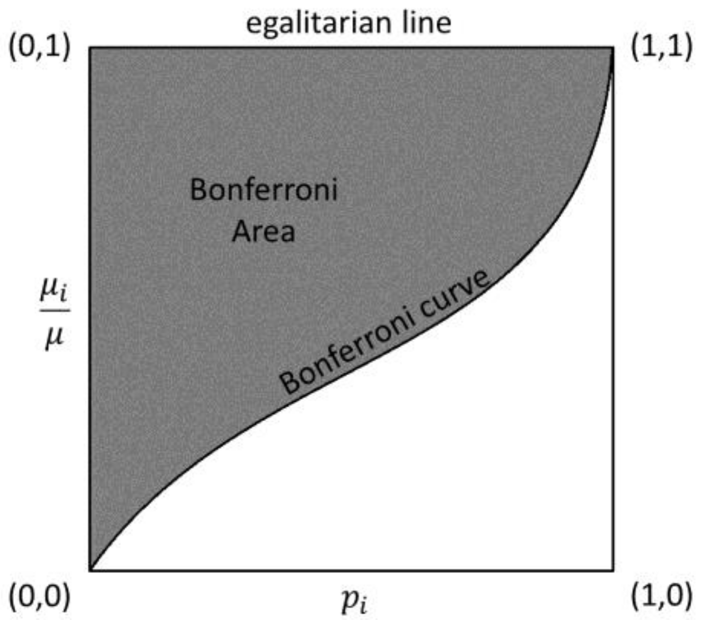
The Bonferroni index is linked to the Bonferroni curve (Figure 2) which is obtained by plotting the cumulative proportion of recipients, arranged in non-decreasing values of income, versus the corresponding ratio between partial mean and total mean ().
The polygonal line joining the points (,) is the Bonferroni curve. If all the recipients in the population have the same income (i.e., equal to ), the Bonferroni curve coincides with the egalitarian line that joins the coordinate points (0,1), (1,). If just a recipient owns the total amount of , the Bonferroni curve is the broken line joining the points (0,0), (,0), (,1).
The value of the Bonferroni index is equal to the ratio between the Bonferroni area—the area between the Bonferroni curve and the egalitarian line—and the Bonferroni area in the case of maximum concentration—the area of the quadrangle defined by the points (0,0), (,0), (1), (0,1). As goes to infinity, the quantity goes to 1 and the Bonferroni area in case of maximum concentration is equal to . Then, the value of coincides with the Bonferroni area (Giorgi and Crescenzi 2001b, pp. 572–73).
3. A Brief Overview on Inequality Index Decomposition
When we consider the decomposition of inequality indices, two main lines of research can be distinguished: decomposition by income sources and by population subgroups (for a comprehensive survey on the subject see, e.g., Giorgi 2011a).
The decomposition by income sources is based on the hypothesis that the total income is the sum of several components, such as wages, salaries, capital incomes, etc. Therefore, the contribution of each source to the overall inequality can be identified. The decomposition by income sources is appealing since the inequality indices can be exactly decomposed into separate components, each one referring to a given factor. Fields (1979a, 1979b) derived the contribution of each source to via so called Factor Inequality Weight (). With slight changes, this method can be adapted to decompose as follows:
where , and are, respectively, the mean income, the share and the value of computed for the -th factor (see, e.g., Tarsitano 1990, p. 236). The is the weight of the -th source which can be referred to as the Bonferroni correlation. In fact, it has the same meaning of the Gini correlation in decomposition. The Bonferroni correlation reflects the degree of concordance between the log-rank ordering of units with respect to the -th income source and the corresponding log-rank order for the total income. In other words, the overall inequality, measured through , depends on the degree of inequality in the distribution of each factor (), the importance of the factor on the total income () and the amount of agreement between the different rankings ().
The decomposition by population subgroups aims at exploring the contribution of individual features such as age, sex, level of education, geographical area, etc., to total inequality (for a deeper investigation on this topic see Deutsch and Silber 1999; Mussard et al. 2006). A first attempt has been proposed by Bhattacharya and Mahalanobis (1967), who tried to decompose by subgroups via an approach based on the analysis of variance. However, cannot be additively decomposed into the sum of between and within components. Mehran (1975) showed that can be decomposed into the sum of within and across components. The difference between the across and the between components is in the interaction component; this is “a measure of the extent of income domination of one group over the other apart from the differences between their mean incomes” (see also Ferrari and Rigo 1987).
As the concentration ratio , the Bonferroni index can be completely decomposed by the sum of three terms:
where is the within component, is the between component and is the interaction component that accounts for the degree of overlap between the income distributions in the different subgroups (for this reason it is also referred to as the overlapping component)2. Therefore, also cannot be additively decomposed (see, e.g., Shorrocks 1980).
4. The Shapley Decomposition
Deutsch and Silber (2007) used the Shapley decomposition introduced, in this field, by Shorrocks (1999), to solve the problem of additive decomposition of by population subgroups. They derived the impact of four components: inequality within subgroups (), inequality between subgroups (), ranking () and relative size in each subgroup ().
The Shapley decomposition is based on the well-known concept of Shapley value in cooperative game theory (Shapley 1953). The idea of the Shapley value is to compute the value of a function considering all the possible combinations of factors. When such a decomposition is applied to inequality indices, and the factors are considered as symmetrical, it allows to derive the expected marginal contribution of each factor to inequality. Moreover, the contributions sum exactly to the amount of the inequality index considered (Shorrocks (1999, 2013)). To decompose , we consider the same factors (i.e., , , , ), used by Deutsch and Silber (2007) for .
Let us assume that a population is partitioned into subgroups () where is the income of the -th recipient () in subgroup . A given inequality measure (for instance, or ) can be seen as a function of the observed incomes, .
In the general case, we may consider within subgroups inequality (), between subgroups inequality () and differences in both the size among the subgroups (, where ) and the rank of recipients . Therefore, the overall inequality can be written as a function of such factors:
The Shapley decomposition may help us derive the marginal impact of each factor measuring the difference in the value of the inequality index corresponding to the observed situation and the reference one, where the income does not change with the factor. Just to give an example, the impact of within subgroups inequality (), is derived by comparing the situations where the incomes of recipients in a given subgroup are different (), to the case when all the recipients in that subgroup have the same income (. To compute the impact of inequality between subgroups , we compare the case when the mean of incomes is different between subgroups () and the case when the average income is constant across subgroups (). To obtain a kind of standardization is applied and is replaced by . To measure the effect of the differences in size (), we compare the case when the subgroups have different sizes () to the case when the sizes are equal (). To make the subgroups have the same size, the least common multiple (lcm) is calculated for the sizes of the analyzed subgroups and the values are repeated lcm times; this leads to equality in size between the subgroups. When applying such an approach to , the objection is usually raised that , as opposed to , does not satisfy the Dalton (1925) principle of being replication invariant. However, using the simulation study reported in Appendix A, we may show that the effect of replications becomes negligible for when the population size is greater than 1000 units. According to this feature, can be defined as being an ‘asymptotically replication invariant’.
Finally, to derive the effect of ranking (), we compare the case when the recipients are sorted by their income to the case when we first sort the subgroups on the basis of their average income, , and then the recipients by their income within each subgroup .
The marginal impact () of each factor on the generic index (either or ) can be derived by computing the following weighted means of the index when, from time to time, the effect of components is removed.
In expressions (5)–(8) by the subscript of we denote the factor that has been removed. For instance, is the index computed when the component of within inequality () has been removed, that is . Furthermore, is the index computed when component of within inequality (), between inequality () have been removed and the recipients are ranked first by the average income of the subgroup they belong and then with respect to their income3.
A Numerical Illustration
To illustrate, we consider a population composed by 10 recipients with income 2, 6, 10, 18, 20, 25, 30, 50, 55, and 84. Let us assume that recipients with income 2, 6 and 25 belong to subgroup A, those with income 10, 20 and 84 to subgroup B and, last, those with income 18, 30, 50 and 55 to subgroup C.
Since this is just an illustrative example of the application of the Shapley decomposition, the replication invariance principle is overlooked. We should remark that, in some cases, when we remove , the corresponding value of can be negative. It occurs when there is a negative correlation between mean income and mean rank (Frick and Jan 2007, p. 10). In fact, in these extreme cases, when sorting the income distribution in decreasing order, as shown by Rao (1969, p. 245), is equal to , and the same occurs for .
Table 1 shows all the scenarios obtained by removing factors separately, in pairs, in set of three and all together. Furthermore, the corresponding income distribution and the values of and are also presented. We report in Table 2 the marginal contributions for each factor () derived using expressions (5)–(8).
5. The Balance of Inequality Approach
The Balance of Inequality, proposed by Di Maio and Landoni (2017), is an alternative approach that, as in the Shapley method, helps solve the problem of additive decomposition of by population subgroups. They use the center mass (or barycenter) to derive a measure of inequality, thus giving a physical interpretation to the inequality measure.
The barycenter of the income distribution, in which in abscissa is the income and in ordinate is the ranking minus one , is defined by the following expression
It is equal to in the case of perfect equality, while it is equal to in the case of maximum inequality. Di Maio and Landoni (2017, p. 12) proceeded to normalize the barycenter and obtained, after a little algebra, the :
Expression (9) corresponds to the Gini concentration index (1) and, for this reason, we will refer to expression (9) as in the following. They show that (9), and therefore the Gini concentration ratio, can be decomposed by considering four factors. Besides those already seen in the previous paragraph—the inequality within and between population subgroups— helps derive the impact on the inequality value due to asymmetry and irregularity of subgroups4. A population (or a subgroup) is symmetrical if the distribution of the analyzed variable is symmetrical with respect to its center. Furthermore, it is regular if the distance between two adjacent individuals in the population or in the subgroup is constant. A regular population (or a subgroup) is also symmetrical.
The for the Gini index can therefore be decomposed as
where is the total income in the -th subgroup; equivalently, we may define the in the -th subgroup via the following expression
where is the rank of the -th recipient in subgroup . Furthermore, is the barycenter of the subgroup in the population in case of perfect inequality, and is the barycenter of the subgroup in the population in the case of perfect equality. In this context, represents the asymmetry effect and the irregularity effect where
is the index for the -th subgroup, while
is the index for the -th subgroup, in the case of symmetrical subgroups.
The first component in expression (10) is the weighted average of the within subgroup inequality, the second is the inequality between subgroups, the third and the fourth are the weighted average of the effects of asymmetry and irregularity of the distribution in each subgroup, respectively.5
The extension of the methodology to the Bonferroni inequality index () requires that we consider a different representation of the income distribution. Let us consider the couple with the income on the abscissa and on the ordinate, where and . The barycenter of this distribution is
It is zero in the case of perfect equality and equal to in the case of maximum inequality. Normalizing the barycenter, as before, and using a little algebra we obtain the expression of in expression (3).
This enable us to apply the approach also to . Expression (11) can be written as
Equivalently
denotes the for the -th subgroup with size , , and where is the rank of recipients in subgroup . Furthermore,
where is the value of corresponding to the recipients with the highest income in subgroup , and denotes the barycenter of the subgroup in the population in case of perfect inequality. The barycenter of the subgroup in the case of perfect equality is
As above, represents the effect of asymmetry while denotes the effect of irregularity on . The index for subgroup is equal to
while the index for a symmetrical subgroup is given by
A Numerical Illustration
Let us consider the same population of 10 recipients we have already discussed in Section 4. We report in Table 3 the contribution of each factor obtained via the balance inequality approach.
By looking at this illustrative example, some preliminary results can be derived. In both cases, the higher contribution to the overall inequality corresponds to the within factor, followed by the between one and other factors. However, we may observe some differences when comparing the current decomposition to the Shapley decomposition in Table 2. The impact of between inequality on is lower when measured with the (30.86% vs. 35.90%), while the impact of within inequality is higher (52.38% vs. 47.02%). On the other hand, when we consider , the values of between inequality are very similar (41.42% vs. 40.13%), while the difference for the within inequality is substantial (59.95% vs. 50.07%). For both indices, asymmetry reduces inequality: this issue is more evident when looking at the decomposition of rather than the one of .
6. An Application to the Italian Income Distribution
The Shapley decomposition of the Gini concentration ratio () and the Bonferroni index () has been applied to income data collected in 2015 by the Italian component of the European Survey on Income and Living Conditions (It-SILC, Istat 2015). The Eu-SILC is a yearly survey carried out by European countries according to the European Regulation n. 1177/2003. Its main aim is to provide data on income, poverty and social exclusion. The 2015 Italian sample is a two-stage sample of municipalities, stratified by population size, and households. The sample size is composed by 17,985 household and 36,602 individuals.
We consider the Italian households as divided into three subgroups, represented by the main geographical areas: North, Center and South. Table 4 shows some explanatory statistics on the distribution of household income for the whole population and the subgroups.
The inequality measures have been computed on the distribution of household income. The incomes have not been equivalized to account for the different households’ size. The values of have been estimated using the expression of the sampling estimator defined by Osier (2009, p. 169), while has been estimated using the expression of the sampling estimator derived in Giorgi and Guandalini (2013, p. 154). The values, for and , have been computed through a plug-in estimator.
Looking at Table 4, we observe that = 0.367 and = 0.462 for the whole population. North and Center have quite a similar situation. While in South the incomes are lower, and the inequality is higher. In the three subgroups, but also at the national level, there is a strong positive asymmetry in the income distribution. The asymmetry is greater in the South when compared to the other geographical areas.
In Table 5, has been decomposed using the Shapley decomposition (as shown in Section 4) and the balance of inequality (as shown in Section 5). As for the Shapley decomposition, it is important to point out that the sample size for all the subgroups is larger than 4000; therefore, the Dalton principle of replication invariance can be considered as (at least approximately) satisfied also for .
The impact of the different factors obtained by the decomposition methods are reported in Table 5. For each component and decomposition, the corresponding confidence interval, estimated via nonparametric bootstrap (= 500 samples), are reported.
The plug-in estimators based on are biased. The bias is negligible for , while it is more evident for . However, this does not affect the comparison between the decomposition methods and the two indices, since, in any case, the bias does not change the balance of power between factors considered obtained via the balance of inequality.
Both decompositions identify the within inequality as a very important factor. Under the Shapley decomposition, it accounts for more than 60% of the whole inequality, both for and . Ranking is more important than between inequality (20% versus 14%), since the subgroups are strongly overlapped. Finally, subgroup size plays a minor role. Under the Shapley decomposition, the magnitude of factors is similar for both the analyzed indices. However, when we consider the impact of within inequality is higher while that of ranking is lower than for . The importance of differences among subgroups in size is negligible when we consider , since it is population size independent, while the same is different from zero in , even if not that high.
Under the decomposition, within inequality accounts for more than 80% of the whole inequality for both the analyzed indices, even if its role is slightly more evident in . Unlike the Shapley decomposition, the two indices show a different “hierarchy” of factors when we look at the corresponding impact. When we consider , the most important factor is the within inequality followed by the between inequality. The contribution of asymmetry and irregularity is almost negligible. On the contrary, when we look at , the asymmetry is the most important factor followed by the within inequality and the irregularity (with a negative sign). Between inequality plays a minor role.
It is important to point out that the combined effect of asymmetry and irregularity has opposite signs on the two indices (0.55 − 2.07 = −1.52% for and 89.13 − 78.00 = 11.13% for ). This is probably due to the indices’ sensitivity to different levels of the income distribution. As remarked above, is more sensitive to lower values (left tail of the distribution), while is more sensitive to the central values of the distribution. Moreover, the high value for the impact of asymmetry and irregularity when we consider can be due to the asymmetry in the income distribution, as already stated, but also to an indirect effect of population size. In fact, as opposed to the numerical illustration in Section 5, the contribution of asymmetry and irregularity to is higher in the It-SILC data due to the larger population size and asymmetry.
The two decomposition methods are deeply different. The Shapley decomposition represents a more general tool which can be used to decompose not only inequality measures and not only by the four factors we have considered here. It can be modified by considering a different (lower or higher) number of factors. The is more similar to a standard decomposition approach, since it is less customizable. In fact it is possible to decompose the index by within inequality, between inequality, asymmetry and irregularity only.
Some Considerations on the Shapley Decomposition and the Balance of Inequality
The numerical examples and the application to real data show that the two decomposition methods point out different aspects of the inequality indices. The Shapley decomposition is more sensitive to the ranking in the income distribution, while the decomposition is more influenced by the shape of the distribution.
Looking at the behavior of the two indices with respect to the adopted decomposition, it is possible to draw some interesting conclusions. Since and adopt a similar ranking system, we cannot observe substantial differences when considering the Shapley decomposition; however, since the indices have different sensitivity to different portions of the distribution, asymmetry and irregularity often play a crucial role in the decomposition, and this may lead to different results.
Finally, as using more synthetic indices can help us highlight differences between socio-economic reality and political significance of inequality (Piketty 2014, p. 156); using more than one decomposition may help focus on different aspects and factors of inequality.
7. Conclusions and Further Research
An important topic on inequality measures is their decomposability. Two main lines of research can be identified: decomposition by income sources and by population subgroups. Some indices, such as the Gini concentration ratio (Gini 1914) and the Bonferroni inequality index (Bonferroni 1930) are not additively decomposable by population subgroups. To overcome this drawback, Deutsch and Silber (2007) proposed the so-called “Shapley value”, and Di Maio and Landoni (2017) suggested the “balance of inequality” () approach to decompose the Gini concentration ratio ().
In this paper, we have discussed the Shapley decomposition for the Bonferroni inequality index (). Furthermore, we also show how the balance of inequality can be extended to . The two indices have been estimated on real data from the 2015 Italian component of the European Survey on Income and Living Conditions (It-SILC) and the two decomposition methods have been considered in this context.
The results of the application highlights that the features of each subpopulation, such as homogeneity within (denoted by the component of within inequality), and the difference in subpopulation size, have higher influence on than on . Furthermore, seems to be more sensitive to asymmetry and irregularity in the observed distribution and the population size.
The two decomposition methods focus on different aspects of the distribution. The Shapley value reflects the ranking in the income distribution, while the is mainly influenced by the shape of the distribution. For these reasons, the two indices have a similar behavior under the Shapley decomposition, as their ranking system is similar, while they may show a completely different “hierarchy” of factors under the balance of inequality decomposition.
The results of our research also suggest the possibility of supplementing the measure of overall inequality through indices with different sensitivity to different parts of the income distribution, trying to answer, at least in part, the possible disadvantages in using a single index (Osberg 2017). This follows, in our view, the path suggested by Piketty (2014, p. 156). Piketty proposed to use different indices to account for the differences between socio-economic reality and political significance of inequality in different parts of the income distribution. In the same way, the use of different kinds of decompositions can help to focus on different aspects and factors of inequality. In this perspective, further studies could focus on the extension of the approach to other indices.
Acknowledgments
The authors would like to thank the Editors and two anonymous reviewers for their valuable comments and suggestions.
Author Contributions
The authors contributed equally to this work.
Conflicts of Interest
The authors declare no conflict of interest.
Appendix A
Let us assume to have a population with a vector of income . Furthermore, let us assume to repeat a finite number of times the income in and define a vector . If is computed on and on , , that is, satisfies the Dalton principle of replication invariance.
When computing on and , usually . Therefore, this is generally intended to show that does not satisfy the Dalton principle of replication invariance. However, this holds for small population sizes (i.e., dimension of ). In fact, it is possible to prove that the difference between and becomes quickly negligible as the population size increases.
The departure of from the Dalton principle of replication invariance can be influenced by three factors: population size, level of concentration and number of replication.
In Table A1, we present the results of a small simulation study. The income for units belonging to twelve populations which differ by size and level of concentration of the corresponding income distribution have been generated from a log-normal distribution. We have considered four values for the population sizes (10, 100, 1000 and 10,000) and three levels of concentration for the corresponding income: low, medium and high, that is about 0.20, 0.50 and 0.80 respectively.
For each population, the index has been computed. Then, the incomes have been replicated 2, 10 and 100 times and has been computed also for the populations with the replicated incomes.
Looking at Table A1, it is clear that does not satisfy the Dalton principle of replication invariance. In fact, the relative differences the value of for populations without replicated incomes and for population with replicated incomes are all non-zero. However, it is possible to note that, generally, the differences are larger when the replications refer to a population with a higher concentration of income distribution. Furthermore, increasing the times of replications contributes to increase the difference between the values of , while, instead, increasing the population size leads to differences going quickly to 0. In all the cases, the differences are negligible to the third decimal place when is greater than 1000. Therefore, it is possible to state that is asymptotically replication invariant.

Table A1.
Values and relative differences of the Bonferroni index () computed for a population with incomes generated by a log-normal distribution and for the same population with incomes replicated 2, 10 and 100 times. For different population sizes (10, 100, 1000, 10,000) and for different concentration of incomes ( 0.20, 0.50 and 0.80).
| Population Size | Relative Difference | ||||||
|---|---|---|---|---|---|---|---|
| Number of Replications | Number of Replications | ||||||
| No Replication | 2 | 10 | 100 | 2 | 10 | 100 | |
| (a) | (b) | (c) | (d) | (b − a)/a | (c − a)/a | (d − a)/a | |
| Low level of concentration ( 0.20) | |||||||
| 10 | 0.30789 | 0.30394 | 0.30183 | 0.30147 | −0.01285 | −0.01971 | −0.02085 |
| 100 | 0.29684 | 0.29692 | 0.29700 | 0.29702 | 0.00025 | 0.00054 | 0.00061 |
| 1000 | 0.29289 | 0.29291 | 0.29292 | 0.29292 | 0.00006 | 0.00011 | 0.00012 |
| 10,000 | 0.28858 | 0.28859 | 0.28860 | 0.28860 | 0.00002 | 0.00004 | 0.00004 |
| Medium level of concentration ( 0.50) | |||||||
| 10 | 0.68310 | 0.67073 | 0.66296 | 0.66145 | −0.01812 | −0.02949 | −0.03170 |
| 100 | 0.64458 | 0.64382 | 0.64323 | 0.64310 | −0.00119 | −0.00210 | −0.00230 |
| 1000 | 0.63418 | 0.63411 | 0.63405 | 0.63404 | −0.00011 | −0.00019 | −0.00021 |
| 10,000 | 0.62732 | 0.62732 | 0.62731 | 0.62731 | −0.00001 | −0.00002 | −0.00002 |
| High level of concentration ( 0.80) | |||||||
| 10 | 0.94323 | 0.91843 | 0.90107 | 0.89744 | −0.02630 | −0.04470 | −0.04855 |
| 100 | 0.88648 | 0.88452 | 0.88298 | 0.88263 | −0.00221 | −0.00395 | −0.00434 |
| 1000 | 0.88150 | 0.88131 | 0.88116 | 0.88113 | −0.00022 | −0.00039 | −0.00043 |
| 10,000 | 0.87653 | 0.87651 | 0.87649 | 0.87649 | −0.00002 | −0.00004 | −0.00004 |
References
- Aaberge, Rolf. 2000. Characterizations of Lorenz Curves and Income Distributions. Social Choice and Welfare 17: 639–53. [Google Scholar] [CrossRef]
- Bárcena-Martin, Elena, and Luis J. Imedio Olmedo. 2008. The Bonferroni, Gini and De Vergottini Indices. Inequality, Welfare and Deprivation in the European Union in 2000. Research on Economic Inequality 16: 231–57. [Google Scholar]
- Bárcena-Martin, Elena, and Jacques Silber. 2011. On the Concepts of Bonferroni Segregation Index Curve. Rivista Italiana di Economia, Demografia e Statistica 62: 57–74. [Google Scholar]
- Bárcena-Martin, Elena, and Jacques Silber. 2013. On the Generalization and Decomposition of the Bonferroni Index. Social Choice and Welfare 41: 763–87. [Google Scholar] [CrossRef]
- Benedetti, Carlo. 1986. Sulla Interpretazione Benesseriale di Noti Indici di Concentrazione e di altri. Metron 45: 421–29. [Google Scholar]
- Bhattacharya, N., and B. Mahalanobis. 1967. Regional Disparities in Household Consumption in India. Journal of the American Statistical Association 62: 143–61. [Google Scholar] [CrossRef]
- Bonferroni, Carlo E. 1930. Elementi Di Statistica Generale. Firenze: Libreria Seber. [Google Scholar]
- Chakravarty, Satya R. 2007. A Deprivation-Based Axiomatic Characterization of the Absolute Bonferroni Index of Inequality. Journal of Economic Theory 5: 339–51. [Google Scholar] [CrossRef]
- Dalton, Hugh D. 1925. Some Aspects of the Inequality of Incomes in Modern Communities. London: Routledge. [Google Scholar]
- De Vergottini, Mario. 1950. Sugli Indici di Concentrazione. Statistica 10: 445–54. [Google Scholar]
- Deutsch, Joseph, and Jacques Silber. 1999. Inequality Decomposition by Population Subgroups and the Analysis of Interdistributional Inequality. In Handbook on Income Inequality Measurement. Edited by Silber Jacques. Boston: Kluwer Academic Publisher, vol. 71, pp. 363–97. [Google Scholar]
- Deutsch, Joseph, and Jacques Silber. 2007. Decomposing Income Inequality by Population Subgroups: A Generalization. In Research on Economic Inequality: Inequality and Poverty. Edited by Bishop John and Amiel Yoram. Berlin: Springer, vol. 14, pp. 237–53. [Google Scholar]
- Di Maio, Giorgio, and Paolo Landoni. 2017. The Balance of Inequality: A Rediscovery of The Gini’s R Concentration Ratio and a New Inequality Decomposition by Population Subgroups Based on Physical Rationale. Paper presented at Seventh Meeting of The Society for the Study of Economic Inequality (Ecineq), New York City, NY, USA, July 17–19. [Google Scholar]
- Ferrari, Guido, and Pietro Rigo. 1987. Sulla Scomposizione del Rapporto di Concentrazione di Gini. In La Distribuzione Personale del Reddito: Problemi di Formazione, di Ripartizione e di Misurazione. Edited by Zenga Michele. Milano: Vita e Pensiero, pp. 347–63. [Google Scholar]
- Fields, Gary S. 1979a. Income Inequality in Urban Colombia: A Decomposition Analysis. Review of Income and Wealth 25: 327–41. [Google Scholar] [CrossRef]
- Fields, Gary S. 1979b. Decomposing LDC Inequality. Oxford Economic Papers 31: 437–59. [Google Scholar] [CrossRef]
- Frick, Joachim R., and Jan Goebel. 2007. Regional Income Stratification in Unified Germany Using a Gini Decomposition Approach. Discussion paper. Berlin, Germany: Germany Institute for Economich Research, 1–32. [Google Scholar]
- Gini, Corrado. 1912. Studi Economico-Giuridici della Facoltà di Giurisprudenza della Regia Università di Cagliari. In Variabilità e Mutabilità: Contributo Allo Studio Delle Distribuzioni e Delle Relazioni Statistiche. Bologna: Cuppini, vol. 3. [Google Scholar]
- Gini, Corrado. 1914. Sulla Misura della Concentrazione e della Variabilità dei Caratteri. Atti Del Reale Istituto Veneto Di Scienze, Lettere ed Arti 73: 1203–48, English Translation In Metron 2005, 63: 3–38. [Google Scholar]
- Giordani, Paolo, and Giovanni M. Giorgi. 2010. A Fuzzy Logic Approach to Poverty Analysis Based on the Gini and Bonferroni Inequality Indices. Statistical Methods and Applications 19: 587–607. [Google Scholar] [CrossRef]
- Giorgi, Giovanni M. 1990. Bibliographic Portrait of the Gini Concentration Ratio. Metron 48: 183–221. [Google Scholar]
- Giorgi, Giovanni M. 1992. Il Rapporto di Concentrazione di Gini. Genesi, Evoluzione ed una Bibliografia Commentata. Siena: Libreria Editrice Ticci. [Google Scholar]
- Giorgi, Giovanni M. 1993. A Fresh Look at the Topical Interest of the Gini Concentration Ratio. Metron 51: 83–98. [Google Scholar]
- Giorgi, Giovanni M. 1998. Concentration Index, Bonferroni. In Encyclopedia of Statistical Sciences. Updated Series; Edited by Kotz Samuel, Read Campbell B. and Banks David L. New York: Wiley-Intersciences, vol. 2, pp. 141–46. [Google Scholar]
- Giorgi, Giovanni M. 1999. Income Inequality Measurement: The Statistical Approach. In Handbook on Income Inequality Measurement. Edited by Silber Jacques. Boston: Kluwer Academic Publishers, pp. 245–60. [Google Scholar]
- Giorgi, Giovanni M. 2005. Gini’s Scientific Work: An Evergreen. Metron 63: 299–315. [Google Scholar]
- Giorgi, Giovanni M. 2011a. The Gini Inequality Index Decomposition, an Evolutionary Study. In The Measurement of Individual Well-Being and Group Inequality: Essay In Memory Of Z.M. Berrebi. London: Routledge, pp. 185–218. [Google Scholar]
- Giorgi, Giovanni M. 2011b. Corrado Gini: The Man and the Scientist. Metron 69: 1–28. [Google Scholar] [CrossRef]
- Giorgi, Giovanni M., and Michele Crescenzi. 2001a. Bayesian Estimation of the Bonferroni Index in a Pareto-Type I Population. Statistical Methods and Applications 10: 41–48. [Google Scholar] [CrossRef]
- Giorgi, Giovanni M., and Michele Crescenzi. 2001b. A Look at the Bonferroni Inequality Measure in a Reliability Framework. Statistica 61: 571–83. [Google Scholar]
- Giorgi, Giovanni M., and Michele Crescenzi. 2001c. A Proposal of Poverty Measures Based on the Bonferroni Inequality Index. Metron 59: 3–15. [Google Scholar]
- Giorgi, Giovanni M., and Alessio Guandalini. 2013. A Sampling Estimator of the Bonferroni Inequality Index. Rivista Italiana di Economia, Demografia e Statistica 67: 151–58. [Google Scholar]
- Giorgi, Giovanni M., and Riccardo Mondani. 1995. Sampling Distribution of Bonferroni Inequality Index from an Exponential Population. Sankhya 57: 10–18. [Google Scholar]
- Imedio Olmedo, Luis J., Elena Bárcena-Martin, and Encarnación M. Parrado-Gallardo. 2012. Income Inequality Indices Interpreted as Measures of Relative Deprivation/Satisfaction. Social Indicator Research 109: 471–91. [Google Scholar] [CrossRef]
- Istat. 2015. Indagine Sulle Condizioni di Vita (UDB IT—SILC). Available online: https://www.istat.it/it/archivio/4152 (accessed on 4 December 2017).
- Kakwani, Nanak C. 1980. Income Inequality and Poverty: Methods of Estimation and Policy Applications. Oxford: Oxford University Press. [Google Scholar]
- Lorenz, Max O. 1905. Method of Measuring the Concentration of Wealth. Publication of the American Statistical Association 9: 209–19. [Google Scholar] [CrossRef]
- Mehran, Farhad. 1975. A Statistical Analysis of Income Inequality Based on a Decomposition of the Gini Index. Bulletin of the International Statistical Institute 46: 145–50, Contributed Paper, 40th Session, Warsaw, Poland. [Google Scholar]
- Mussard, Stéphane, Françoise Seyte, and Michel Terrazza. 2006. La Décomposition de l’Indicateur de Gini en Sous Groupes: Une Revue de la Littérature. GRÉDI Working paper 06-11. Sherbrooke, QC, Canada: Université De Sherbrooke. [Google Scholar]
- Nygård, Fredrik, and Arne Sandström. 1981. Measuring Income Inequality. Stockholm: Almqvist & Wiksell International. [Google Scholar]
- Osberg, Lars. 2017. On the Limitations of Some Current Usages of the Gini Index. Review of Income and Wealth 63: 574–84. [Google Scholar] [CrossRef]
- Osier, Guillaume. 2009. Variance Estimation for Complex Indicators of Poverty and Inequality Using Linearization Techniques. Survey Research Methods 3: 167–95. [Google Scholar]
- Piesch, Walter. 1975. Statistische Konzentrationsmasse. Tübingen: J.B.C. Mohr (Paul Siebeck). [Google Scholar]
- Piketty, Thomas. 2014. Capital in the Twenty-First Century. Cambridge: Harvard University Press. [Google Scholar]
- Pizzetti, Ernesto. 1951. Relazioni fra Indici di Concentrazione. Statistica 11: 294–316. [Google Scholar]
- Rao, V. 1969. Two Decompositions of Concentration Ratio. Journal of the Royal Statistical Society 132: 418–25. [Google Scholar] [CrossRef]
- Shapley, Lloyd. 1953. A Value for N-Person Games. In Contributions to the Theory of Games (AM-28). Edited by Kuhn Harold W. and Tucker Albert W. Princeton: Princeton University Press, vol. 2, pp. 307–18. [Google Scholar]
- Shorrocks, Anthony F. 1980. The Class of Additively Decomposable Measures. Econometrica 48: 613–25. [Google Scholar] [CrossRef]
- Shorrocks, Anthony F. 1999. Decomposition Procedures for Distributional Analysis: A Unified Framework Based on the Shapley Value. Essex, UK: Department of Economics, University of Essex. [Google Scholar]
- Shorrocks, Anthony F. 2013. Decomposition Procedures for Distributional Analysis: A Unified Framework Based on the Shapley Value. The Journal of Economic Inequality 11: 99–126. [Google Scholar] [CrossRef]
- Silber, Jacques, and Hyun Son. 2010. On the Link between the Bonferroni Index and the Measurement of Inclusive Growth. Economics Bulletin 30: 421–28. [Google Scholar]
- Tarsitano, Agostino. 1990. The Bonferroni Index of Income Inequality. In Income and Wealth Distribution, Inequality and Poverty. Edited by Dagum Camilo and Zenga Michele. Berlin: Springer, pp. 228–42. [Google Scholar]
- Yitzhaki, Shlomo. 1998. More than a dozen alternative ways of spelling Gini. Research on Economic Inequality 8: 13–30. [Google Scholar]
| 1 | In expression (3) the summation is limited to and then divided by . This formulation is different from the one used in other papers mentioned in the Introduction (where the summation is up to the division by is used). Of course, increasing , and the last term in the summation is null. |
| 2 | For the expressions of , and in the case of income classes, see Tarsitano (1990), while for the matrix decomposition of see Bárcena-Martin and Silber (2013). |
| 3 | In expressions (5)–(8), because all the inequality factors have been removed. |
| 4 | Di Maio and Landoni (2017) consider the asymmetry and the irregularity as a unique factor but, to investigate the differences between and , it could be useful to consider them separately. |
| 5 | For more detail on see Di Maio and Landoni (2017). |
Figure 1.
An example of the Lorenz curve in the continuous case (i.e., goes to infinity).
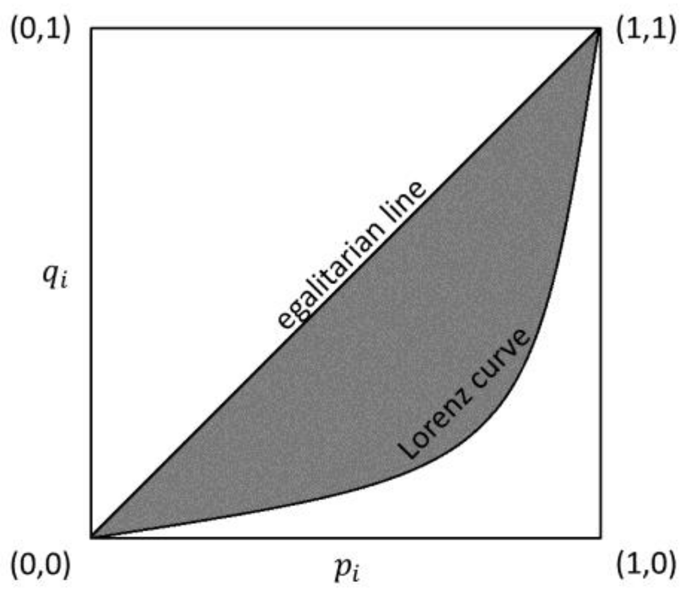
Figure 2.
An example of the Bonferroni curve in the continuous case (i.e., goes to infinity).

Table 1.
Gini concentration ratio () and Bonferroni inequality index () in different scenarios according to factors that have been removed. Illustrative example on the income of 10 recipients from three different subgroups: A = {2, 6, 25} and B = {10, 20, 84}, C = {18, 30, 50, 55}.
Table 1.
Gini concentration ratio () and Bonferroni inequality index () in different scenarios according to factors that have been removed. Illustrative example on the income of 10 recipients from three different subgroups: A = {2, 6, 25} and B = {10, 20, 84}, C = {18, 30, 50, 55}.
| Removed Factor | Income Distribution | |||
|---|---|---|---|---|
| 1 | 2, 6, 10, 18, 20, 25, 30, 50, 55, 84 | 0.490 | 0.609 | |
| 2 | 11, 11, 38, 38.25, 38, 11, 38.25, 38.25, 38.25, 38 | 0.151 | 0.252 | |
| 3 | 5.45, 16.36, 7.89, 14.12, 15.79, 68.18, 23.53, 39.22, 43.14, 66.32 | 0.360 | 0.475 | |
| 4 | 2, 2, 2, 2, 6, 6, 6, 6, 10, 10, 10, 10, 18, 18, 18, 20, 20, 20, 20, 25, 25, 25, 25, 30, 30, 30, 50, 50, 50, 55, 55, 55, 84, 84, 84, 84 | 0.474 | 0.612 | |
| 5 | 2, 6, 25, 10, 20, 84, 18, 30, 50, 55 | 0.333 | 0.481 | |
| 6 | 30, 30, 30, 30, 30, 30, 30, 30, 30, 30, 30, 30 | 0.000 | 0.000 | |
| 7 | 11, 11, 11, 11, 11, 11, 11, 11, 11, 38, 38, 38, 38.25, 38.25, 38.25 38, 38, 38, 38, 11, 11, 11, 11, 38.25, 38.25, 38.25, 38.25, 38.25, 38.25, 38.25, 38.25, 38.25, 38.25, 38, 38, 38 | 0.167 | 0.283 | |
| 8 | 11, 11, 11, 38, 38, 38, 38.25, 38.25, 38.25, 38.25 | 0.212 | 0.331 | |
| 9 | 5.45, 5.45, 5.45, 5.45, 16.36, 16.36, 16.36, 16.36, 27.27, 7.89, 7.89, 7.89, 14.12, 14.12, 14.12, 15.79, 15.79, 15.79, 15.79, 68.18, 68.18, 68.18, 68.18, 23.53, 23.53, 23.53, 39.22, 39.22, 39.22, 43.14, 43.14, 43.14, 65.88, 66.32, 66.32, 66.32 | 0.334 | 0.466 | |
| 10 | 5.45, 16.36, 68.18, 7.89, 15.79, 66.32, 14.12, 23.53, 39.22, 43.14 | 0.128 | 0.233 | |
| 11 | 2, 2, 2, 2, 6, 6, 6, 6, 25, 25, 25, 25, 10, 10, 10, 10, 20, 20, 20, 20, 84, 84, 84, 84, 18, 18, 18, 30, 30, 30, 50, 50, 50, 55, 55, 55 | 0.331 | 0.501 | |
| 12 | 30, 30, 30, 30, 30, 30, 30, 30, 30, 30, 30, 30, 30, 30, 30, 30, 30, 30, 30, 30, 30, 30, 30, 30, 30, 30, 30, 30, 30, 30, 30, 30, 30, 30, 30, 30 | 0.000 | 0.000 | |
| 13 | 30, 30, 30, 30, 30, 30, 30, 30, 30, 30, 30, 30 | 0.000 | 0.000 | |
| 14 | 11, 11, 11, 11, 11, 11, 11, 11, 11, 11, 11, 11, 38, 38, 38, 38, 38, 38, 38, 38, 38, 38, 38, 38, 38.25, 38.25, 38.25, 38.25, 38.25, 38.25, 38.25, 38.25, 38.25, 38.25, 38.25, 38.25 | 0.214 | 0.343 | |
| 15 | 5.45, 5.45, 5.45, 5.45, 16.36, 16.36, 16.36, 16.36, 68.18, 68.18, 68.18, 68.18, 7.89, 7.89, 7.89, 7.89, 15.79, 15.79, 15.79, 15.79, 66.32, 66.32, 66.32, 66.32, 14.12, 14.12, 14.12, 23.53, 23.53, 23.53, 39.22, 39.22, 39.22, 43.14, 43.14, 43.14 | 0.127 | 0.259 | |
| 16 | 30, 30, 30, 30, 30, 30, 30, 30, 30, 30, 30, 30, 30, 30, 30, 30, 30, 30, 30, 30, 30, 30, 30, 30, 30, 30, 30, 30, 30, 30, 30, 30, 30, 30, 30, 30 | 0.000 | 0.000 | |
Note: = inequality within; = inequality between; = size; = ranking.
Table 2.
Marginal impact of factors on Gini concentration ratio () and Bonferroni inequality index (). Illustrative example on the income of 10 recipients from three different population subgroups: A = {2, 6, 25} and B = {10, 20, 84}, C = {18, 30, 50, 55}.
Table 2.
Marginal impact of factors on Gini concentration ratio () and Bonferroni inequality index (). Illustrative example on the income of 10 recipients from three different population subgroups: A = {2, 6, 25} and B = {10, 20, 84}, C = {18, 30, 50, 55}.
| Factor | Contribution to | Contribution to | ||
|---|---|---|---|---|
| % | % | |||
| within inequality | 0.230 | 47.02 | 0.305 | 50.07 |
| between inequality | 0.176 | 35.90 | 0.244 | 40.13 |
| size | 0.005 | 1.00 | −0.007 | −1.22 |
| ranking | 0.079 | 16.07 | 0.067 | 11.02 |
| Total | 0.490 | 100.00 | 0.609 | 100.00 |
Table 3.
Balance of inequality decomposition for the Gini concentration ratio () and the Bonferroni inequality index (). Illustrative example on the income of 10 recipients from three different population subgroups: A = {2, 6, 25} and B = {10, 20, 84}, C = {18, 30, 50, 55}.
Table 3.
Balance of inequality decomposition for the Gini concentration ratio () and the Bonferroni inequality index (). Illustrative example on the income of 10 recipients from three different population subgroups: A = {2, 6, 25} and B = {10, 20, 84}, C = {18, 30, 50, 55}.
| Factor | Contribution to | Contribution to | ||
|---|---|---|---|---|
| % | % | |||
| within inequality | 0.256 | 52.38 | 0.365 | 59.95 |
| between inequality | 0.151 | 30.86 | 0.252 | 41.42 |
| asymmetry | −0.007 | −1.35 | −0.025 | −4.10 |
| irregularity | 0.010 | 2.05 | 0.017 | 2.73 |
| Total | 0.490 | 100.00 | 0.609 | 100.00 |
Table 4.
Some explanatory statistics on average Italian household income distribution by three subgroups (North, Center and South). Source: It-SILC, Italy 2015.
Table 4.
Some explanatory statistics on average Italian household income distribution by three subgroups (North, Center and South). Source: It-SILC, Italy 2015.
| Geographical Area | Households | First Quartile | Median | Mean | Third Quartile | Fisher Asymmetry Coefficient | R | B | |
|---|---|---|---|---|---|---|---|---|---|
| Sample Size | Population Size | ||||||||
| North | 8922 | 12,294,699 | 25,809 | 39,180 | 47,621 | 59,749 | 4.273 | 0.346 | 0.439 |
| Center | 4223 | 5,295,623 | 23,114 | 36,459 | 44,626 | 56,524 | 2.379 | 0.360 | 0.457 |
| South | 4840 | 8,185,550 | 16,939 | 26,617 | 32,561 | 40,400 | 10.861 | 0.372 | 0.482 |
| Italy | 17,985 | 25,775,872 | 22,007 | 34,199 | 42,223 | 53,480 | 5.143 | 0.367 | 0.462 |
Table 5.
Shapley and Balance of inequality decompositions for the Gini concentration ratio () and the Bonferroni inequality index (). Application to Italian household income distribution by three population subgroups (North, Center and South). Source: It-SILC, Italy 2015.
Table 5.
Shapley and Balance of inequality decompositions for the Gini concentration ratio () and the Bonferroni inequality index (). Application to Italian household income distribution by three population subgroups (North, Center and South). Source: It-SILC, Italy 2015.
| Factor | Contribution to | Contribution to | ||
|---|---|---|---|---|
| Absolute Value | % | Absolute Value | % | |
| Shapley decomposition | ||||
| within inequality | 0.2348 | 63.99 | 0.3065 | 66.30 |
| [0.2281, 0.2415] | [62.16, 65.80] | [0.2956, 0.3174] | [63.94, 68.66] | |
| between inequality | 0.0530 | 14.44 | 0.0626 | 13.55 |
| [0.0439, 0.0621] | [11.95, 16.93] | [0.0522, 0.0730] | [11.28, 15.80] | |
| size | −0.0002 | −0.05 | 0.0090 | 1.95 |
| [−0.0037, 0.0033] | [−1.00, 0.89] | [0.0046, 0.0134] | [0.99, 2.90] | |
| ranking | 0.0793 | 21.62 | 0.0841 | 18.20 |
| [0.0700, 0.0886] | [19.08, 24.13] | [0.0757, 0.0925] | [16.37, 20.01] | |
| Total | 0.3670 | 100.00 | 0.4623 | 100.00 |
| [0.3568, 0.3772] | [0.4505, 0.4741] | |||
| Balance of Inequality () | ||||
| within inequality | 0.3483 | 94.98 | 0.4007 | 81.07 |
| [0.3384, 0.3582] | [94.89, 95.02] | [0.3908, 0.4106] | [79.07, 83.09] | |
| between inequality | 0.0239 | 6.54 | 0.0385 | 7.79 |
| [0.0182, 0.0296] | [5.11, 7.85] | [0.0293, 0.0477] | [6.05, 9.65] | |
| asymmetry | 0.0020 | 0.55 | 0.4405 | 89.13 |
| [0.0008, 0.0032] | [0.24, 0.84] | [0.4393, 0.4417] | [90.78, 89.36] | |
| irregularity | −0.0076 | −2.07 | −0.3855 | −78.00 |
| [−0.0095, −0.0057] | [−2.65, −1.52] | [−0.3874, −0.3836] | [−80.04, −77.62] | |
| Total | 0.3668 | 100.00 | 0.4942 | 100.00 |
| [0.3566, 0.3770] | [0.3908, 0.4106] | |||
Note: Bootstrap confidence interval at 95% in squared brackets.
© 2018 by the authors. Licensee MDPI, Basel, Switzerland. This article is an open access article distributed under the terms and conditions of the Creative Commons Attribution (CC BY) license (http://creativecommons.org/licenses/by/4.0/).
Share and Cite
MDPI and ACS Style
Giorgi, G.M.; Guandalini, A. Decomposing the Bonferroni Inequality Index by Subgroups: Shapley Value and Balance of Inequality. Econometrics 2018, 6, 18. https://0-doi-org.brum.beds.ac.uk/10.3390/econometrics6020018
AMA Style
Giorgi GM, Guandalini A. Decomposing the Bonferroni Inequality Index by Subgroups: Shapley Value and Balance of Inequality. Econometrics. 2018; 6(2):18. https://0-doi-org.brum.beds.ac.uk/10.3390/econometrics6020018
Chicago/Turabian StyleGiorgi, Giovanni M., and Alessio Guandalini. 2018. "Decomposing the Bonferroni Inequality Index by Subgroups: Shapley Value and Balance of Inequality" Econometrics 6, no. 2: 18. https://0-doi-org.brum.beds.ac.uk/10.3390/econometrics6020018
Note that from the first issue of 2016, this journal uses article numbers instead of page numbers. See further details here.