Decomposing Wage Distributions Using Recentered Influence Function Regressions

1
Insper Institute of Education and Research, R. Quatá, 300, São Paulo–SP 04546-042, Brazil
2
Vancouver School of Economics, University of British Columbia, 6000 Iona Drive, Vancouver, BC V6T 1L4, Canada
*
Author to whom correspondence should be addressed.
Econometrics 2018, 6(2), 28; https://0-doi-org.brum.beds.ac.uk/10.3390/econometrics6020028
Submission received: 31 December 2017
/
Revised: 27 April 2018
/
Accepted: 9 May 2018
/
Published: 25 May 2018
(This article belongs to the Special Issue Econometrics and Income Inequality)
Abstract
:This paper provides a detailed exposition of an extension of the Oaxaca-Blinder decomposition method that can be applied to various distributional measures. The two-stage procedure first divides distributional changes into a wage structure effect and a composition effect using a reweighting method. Second, the two components are further divided into the contribution of each explanatory variable using recentered influence function (RIF) regressions. We illustrate the practical aspects of the procedure by analyzing how the polarization of U.S. male wages between the late 1980s and the mid 2010s was affected by factors such as de-unionization, education, occupations, and industry changes.
1. Introduction
The ongoing growth in wage inequality in the United States and several other countries over the past thirty-five years has generated a resurgence of interest for distributional issues and methods to analyze these issues. There is also a sizeable literature looking at wages differentials between subgroups that goes beyond simple mean comparisons. More generally, there is increasing interest in distributional impacts of various programs or interventions. In all these cases, the key question of economic interest is which factors account for changes (or differences) in distributions. For example, did wage inequality increase because education or other wage setting factors became more unequally distributed, or because the return to these factors changed over time?
In response to these important questions, several decomposition procedures have been suggested to untangle the sources of changes or differences in wage distributions. In Fortin et al. (2011), we reviewed the traditional Oaxaca-Blinder (OB) decomposition method and several of its extensions in the context of the treatment effect literature to highlight the advantages and disadvantages of different methodologies. The goal of the current paper is to provide a detailed and updated exposition of an extension to the OB decomposition that relies on recentered influence function (RIF) regressions (Firpo et al. 2009) [FFL, thereafter] to estimate the effect of covariates on inequality measures, such as percentile differences and ratios, the variance of log wages, or the Gini coefficient.1 Relative to several procedures proposed recently (Machado and Mata 2005; Melly 2005; Chernozhukov et al. 2013) [CFM, thereafter], this method has the advantage of allowing general distributional measures to be decomposed non-sequentially in the same way means can be decomposed using the conventional OB method. The methodology has been applied in a number of different settings where the object of interest is the unconditional distribution of outcomes.2
As is well known, the OB procedure provides a way of: (1) decomposing changes or differences in mean wages into a wage structure effect and a composition effect; and (2) further dividing these two components into the contribution of each covariate. The main problem with sequential decomposition methods is that they cannot be used to divide the composition effect into the role of each covariate in a way that is independent of the order of the decomposition. Thus, while it is natural to ask to what extent changes in the distribution of education have contributed to the growth in wage inequality, this particular question has not been answered in the literature for lack of available decomposition methods. In contrast, this question is straightforward to answer in the case of the mean using a OB decomposition.
In this paper, we focus on a two-stage procedure that can be used to perform OB type decompositions on any distributional measure, and not only the mean. The first stage consists of decomposing the distributional statistic of interest into a wage structure and a composition component using a reweighting approach, where the weights are either parametrically or non-parametrically estimated. As in the related program evaluation literature, we show that ignorability and common support are key assumptions required to identify separately the wage structure and composition effects. Provided that these assumptions are satisfied, the underlying wage setting model can be as general as possible. The idea of the first stage is thus very similar to DiNardo et al. (1996). Here, we clarify the assumptions required for the identification of distributional statistics besides the mean by drawing a parallel with the program evaluation (treatment effect) literature.
In the second stage, we further divide the wage structure and composition effects into the contribution of each covariate, just as in the usual OB decomposition. This is done using the regression-based method proposed by FFL to estimate the effect of changes in covariates on any distributional statistics such as inter-quartile ranges, the variance, or the Gini coefficient.
The method developed in FFL replaces the dependent variable of a regression by the corresponding recentered influence function (RIF) for the distributional statistics of interest. The influence function, also known as Gâteaux (1913) derivative, is a widely used concept in robust statistics and is easy to compute. Using the fact that the expected value of the influence function is equal to zero and the law of iterated expectations, we can express the distributional statistic of interest as the average of the conditional expectation of the RIF given the covariates. As in FFL, we call these conditional expectations RIF-regressions.
Average derivatives computed using the RIF-regressions yield the partial effect of a small location shift in the distribution of covariates on the distributional statistic of interest. FFL call this parameter Unconditional Partial Effect (UPE), which for the special case of quantiles become the Unconditional Quantile Partial Effect (UQPE). By approximating the conditional expectations by linear functions, the coefficients of these RIF-regressions indicate by how much the functional (e.g., the quantile) of the marginal outcome distribution is affected by an infinitesimal shift to the right in the distribution of the regressors.
Because the UPE parameter corresponds to the effect of infinitesimal shift in the distribution of regressors, it approximates well small changes in that distribution, but not necessarily large changes. For known changes in the distribution of covariates (e.g., between two time periods), one can easily compute the associated total change in the functional of the outcome distribution of interest. Rothe (2012) proposes statistical inference for that case.3 Both Rothe (2012) and CFM compute the conditional CDF (cumulative distribution function) of the outcome given covariates in the first step. This adds a computationally intensive layer of estimation, since one needs to calculate the entire conditional CDF, even if only interested in one single quantile of the marginal outcome distribution. By contrast, our approach requires only one OLS regression, which is very attractive from a computational standpoint. Finally, even though we end up performing bootstrap-based inference in our empirical application, we show in the Appendix B that the analytical formulas for the standard errors of the reweighting estimates can be derived.
The main advantage of using the RIF-regression method in a Oaxaca-Blinder type decomposition is that it provides a linear approximation of highly non-linear functionals, such as the quantiles or the Gini coefficient. Nevertheless, its simplicity comes at a cost. As pointed out by Rothe (2015), the impact of changes in the distribution of covariates on some non-linear functionals may be poorly approximated by RIF-regressions. Thus, approximation errors are a by-product of the method and they should always be reported in the decomposition results, as we do in our empirical analysis below.
We illustrate how our procedure works in practice by looking at changes in the distribution of male wages in the United States between the late 1980s and the mid 2010s. This period is quite interesting from a distributional point of view as inequality increased in the top end of the wage distribution, but decreased in the low end of the distribution, a phenomenon that Autor et al. (2006) referred to as the polarization of the U.S. labor market. We use our method to investigate the source of change in the wage distribution by decomposing the changes at various wage quantiles. The results indicate that no single factor appears to be able to fully explain the polarization of the wage distribution. De-unionization accounts for some of the decreasing wage inequality at the low end and increasing inequality at the top end. The continuing growth in returns to education, especially at a level above high school, is the most important source of growth in top-end inequality. Changes in the occupational structure of the workforce helps account for the polarization of wages, but these wage changes are mostly offset by changes in the effect of industry at the upper end of the distribution. This explains why, despite convincing evidence that the “routinization of jobs” had substantial impact of the polarization of employment, its effects of wage polarization has been more difficult to identify directly (e.g., Autor and Dorn 2013). Our results suggest that the wage decline in “routine occupations” (Autor et al. 2003), such as production jobs in the manufacturing sector, has been compensated by increases in the primary sector (e.g., mining, oil and gas, etc.), the distribution sector (transportation and wholesale) and in the services sector. Potentially offsetting effects underline the need for the proposed approach that can “run horse races" between different sets of factors. However, increases at the lower end appear to be attributable to changes in minimum wages, which we do not model here.4
The remainder of the paper is organized as follows. Section 2 discusses the decomposition problem and reviews the strengths and weaknesses of existing procedures. The identification of the proposed decomposition procedure is presented in Section 3. Section 4 discusses estimation and inference, and illustrates how the decomposition methodology works in the case of quantiles, the variance, and the Gini coefficient. Section 5 provides an empirical application of the methodology to the changes in the distribution of male wages in the United States between the late 1980s and the mid 2000s.
2. The Decomposition Problem and Shortcomings of Existing Methods
Before presenting our method in detail, it is useful to first review the case of the mean for which the standard OB method is very well known. To simplify the exposition, we will work with the case where the outcome variable, Y, is the wage, although our approach can be used for any other outcome variable. The OB method can be used to divide a difference in mean wages between two groups, or overall mean wage gap, into a composition effect linked to differences in covariates between the two groups, and a wage structure effect linked to differences in the return to these covariates between the two groups. The two groups are labeled as . In the original papers by Oaxaca (1973) and Blinder (1973), the two groups used were either men and women, or blacks and whites. More generally, the two groups can be a control and a treatment group, or similar groups of individuals at two points in time, as in the wage inequality literature.
We first review how the OB decomposition provides a straightforward way of dividing up the contribution of each covariate in a composition and a wage structure effect. Focusing on differences in the wage distributions of two groups, 1 and 0, for a worker i, let be the wage that would be paid in Group 1, and the wage that would be paid in Group 0. Since a given individual i is only observed in one of the two groups, we either observe or , but never both. Therefore, for each i, we can define the observed wage, , as , where if individual i is observed in Group 1, and if individual i is observed in group 0. There is also a vector of covariates that we can observe in both groups.
In the standard OB decomposition, one assumes a linear functional form. In other words, one writes
where .
Define the overall mean wage gap as = , and consider dividing the overall mean gap into a wage structure effect and a composition effect. Averaging over X, the mean wage gap can be written as
where because , so the expression reduces to = − . Thus, by adding and subtracting we get
The first term in the equation is the wage structure effect, , while the second term is the composition effect, . Note that the reference group used to compute the wage structure effect here is the Group 0, though the decomposition could also be performed using Group 1 instead as the reference group. The wage structure and composition effects can also be written in terms of sums over the explanatory variables
where and represent the kth element of X and , respectively. This provides a simple way of dividing and into the contribution of a single covariate or a group of covariates as needed.
Because of the linearity assumption, the OB decomposition is very easy to compute in practice. It can be estimated by replacing the parameter vectors by their OLS estimates, and replacing the expected value of the covariates by the sample averages.
There are nonetheless some important limitations to the standard OB decomposition. A well-known difficulty discussed by Oaxaca and Ransom (1999) and Gardeazabal and Ugidos (2004) is that the contribution of each covariate to the wage structure effect, , is sensitive to the choice of the base group.5
A second limitation discussed by Barsky et al. (2002) is that the OB decomposition provides consistent estimates of the wage structure and composition effect only under the assumption that the conditional expectation is linear.6 One possible solution to the problem is to estimate the conditional expectation using non-parametric methods. Another solution proposed by Barsky et al. (2002) is to use a (non-parametric) reweighting approach as in DiNardo et al. (1996) to perform the decomposition.7 The advantage of this solution is that it can be applied to more general distributional statistics. The disadvantage of both solutions, however, is that they do not provide direct ways, in general, of further dividing the contribution of each covariate to the wage structure and composition effects.8
Currently available methods, such as DiNardo et al. (1996), can be used to compute the overall wage structure and composition effects for various distributional statistics. We build on this in the current paper by suggesting to estimate these two overall effects using a reweighting procedure. Available methods are much more limited, however, when it comes to further dividing the wage structure and, especially, the composition effect into the contribution each covariate. The main contribution of the paper is to explain how a simple regression-based procedure to remedy this shortcoming building on recent work by FFL.
3. Identification of General Composition and Structure Effects
3.1. Wage Structure and Composition Effects
Following the treatment effect literature (Rosenbaum and Rubin 1983, Heckman 1990, Heckman and Robb 1985, 1986), we focus on differences in the wage distributions between two groups, 1 and 0. Suppose we could observe a random sample of individuals, where and are the number of individuals in each group and we index individuals by . We define the probability that an individual i is in Group 1 as p, whereas the conditional probability that an individual i is in Group 1 given , is , sometimes simply called the propensity score.
Wage determination depends on some observed components and on some unobserved components through the wage structure functions
where are unknown real-valued mappings: As we are not imposing any distribution assumption or specific functional form, writing and in this way does not restrict the analysis in any sense. We will however assume that , or equivalently , have an unknown joint distribution but that is far from being restrictive.
From observed data on , we can non-parametrically identify the distributions of and . Without further assumptions, however, we cannot identify the counterfactual distribution of . The counterfactual distribution is the one that would have prevailed under the wage structure of Group 0, but with the distribution of observed and unobserved characteristics of Group 1. For the sake of completeness, we consider also the conditional distributions , and .
We typically analyze the difference in wage distributions between Groups 1 and 0 by looking at some functionals of these distributions. Let be a functional of the conditional joint distribution of , that is , and is a class of distribution functions such that if . The difference in the s between the two groups is called here the -overall wage gap, which is basically the difference in wages measured in terms of the distributional statistic :9
We can use the fact that the distribution of X is not the same across groups to decompose Equation (2) into two parts:
where the second term reflects the effect of differences in the distribution of X.
The first term of the sum, , will reflect changes in the functions only if we are able to fix the distribution of observables and unobservables as the one prevailing for Group 1, that is, the distribution of . For that to be true, will be a functional evaluated at that distribution. This holds under the following assumptions: Ignorability and Overlapping Support.
The Ignorability Assumption has become popular in empirical research following a series of papers by Rubin and coauthors and by Heckman and coauthors.10 In the program evaluation literature, this assumption is sometimes called unconfoundedness and allows identification of the treatment effect on the treated sub-population.
Assumption 1.
: Let have a joint distribution. For all x in : ε is independent of T given
The Ignorability assumption should be analyzed in a case-by-case situation, as it is more plausible in some cases than in others. In our case, it states that the distribution of the unobserved explanatory factors in the wage determination is the same across Groups 1 and 0, once we condition on a vector of observed components.11 Now, consider the following assumption about the support of the covariates distribution:
Assumption 2.
: For all x in , Furthermore,
The Overlapping Support assumption requires that there be an overlap in observable characteristics across groups, in the sense that there is no value of x in such that it is only observed among individuals in Group 1.12 Under these two assumptions, we are able to identify the parameters of the counterfactual distribution of . To see how the identification result works, let us define first three relevant weighting functions:
The first two reweighting functions transform features of the marginal distribution of Y into features of the conditional distribution of given , and of given . The third reweighting function transforms features of the marginal distribution of Y into features of the counterfactual distribution of given . We are now able to state our first identification result:13
Result 1.
:
Under Assumptions 1 and 2:
(i)
()
Identification of implies identification of and therefore of and . Furthermore, because of the ignorability assumption, we know that differences between the conditional distributions of and correspond only to differences in the conditional distributions and . Thus, will only reflect changes in distribution of X. We state these results more precisely below.
Result 2.
:
Under Assumptions 1 and 2:
(i) , are identifiable from data on ();
() if then ;14
() if , then
In Result 2, the identification of and follows from the fact that these quantities can be expressed as functionals of the distributions obtained by weighting the observations with the inverse probabilities of belonging to Group 0 or 1 given T, as stated in Result 1. Note that the non-parametric identification of either the wage determination functions and , or the distribution function of are not necessary for the effects and to be identified. Therefore, methods based on conditional mean restrictions (the OB decomposition approach) and methods based on conditional quantile restrictions (the Machado and Mata (2005) approach) are based on too strong identification conditions that can be easily relaxed if we are simply interested in the terms and .
Part () of Result 2 also states that, when there are no group differences in the wage determination functions, then we should find no wage structure effects. Part () states that, if there are no group differences in the distribution of the covariates, there will be no composition effects.
Finally, it is interesting to relate these general results to the OB decomposition. Given the functional form assumptions of OB, the conditional mean zero expectation of and ignorability assumption, it follows that equals , the counterfactual mean or the expectation of given :
In the following subsection, we show how one can generalize other features of the OB decomposition using a regression based approach, the RIF Regression.
3.2. The RIF Regressions
One important goal of the desired approach, as discussed in Section 2, is to apportion the wage structure and composition effects into the contribution of each individual covariate. To do so, we use the method proposed by FFL to compute partial effects of changes in distribution of covariates on a given functional of the distribution of . The method works by providing a linear approximation to a non-linear functional of the distribution. Thus, through collecting the leading term of a von Mises (1947) expansion, FFL approximate those non-linear functionals by expectations, which are linear functionals or statistics of the distribution. Finally, that linearization method allows one to apply the law of iterated expectations to the distributional statistics of interest and thus to compute approximate partial effects of changes in the distribution of each single covariate on the functional of interest.
The details of the method are summarized as follows. Consider again a general functional . Recall the definition of the influence function (Hampel 1974), , introduced as a measure of robustness of to outlier data when F is replaced by the empirical distribution: , where , and where is a distribution that only puts mass at the value y. It can be shown that, by definition, .
We use a recentered version of the influence function that has an expectation equal to the original :
Letting and , we can therefore write the distributional statistics , , and as the expectations: , and . Using the law of iterated expectations, the distributional statistics can also be expressed in terms of expectations of the conditional recentered influence functions
Letting the so-called RIF-regressions be written as , for , and , we have
It follows that and can be rewritten as:
As is well known, in the case of the mean, the influence function at point y is its deviation from the mean and, therefore, the recentered influence function of the mean is simply the point y itself
As a result, the RIF-regression coefficients in the case of the mean are identical to standard regression coefficients of Y on X used in the OB decomposition ( above), and we have
where , and
where is an approximation error. When the linearity and zero conditional mean assumption of the OB decomposition are satisfied, it follows that and , as seen in the end of the previous subsection. Our decomposition is then identical to the OB decomposition. However, when these conditions are not satisfied the two decompositions are different.
In general, there is no particular reason to expect the conditional expectations and to be linear in X. As a matter of convenience and comparability with OB decompositions, it is nonetheless useful to consider the case of the linear specification. To be more precise, consider the linear projections (indexed by L)
where
As is well known, even though linear projections are only an approximation for the true conditional expectation, the expected approximation error is zero, so that:
We can thus rewrite and as:
which generalizes the OB decomposition to any distributional statistic through the projection of its recentered influence function onto the covariates. Note that, under an additional assumption that and , that is, if the conditional expectation is indeed linear in x, then . In the case of the mean (), it then follows that the equations above reproduce exactly the OB decomposition.
It is important to note that the case of the mean is quite unique because the recentered influence function does not depend on the distribution F, i.e., . The lack of dependence on F is due to the fact that the influence function is a linear approximation that is exact in the case of the mean. For other distributional statistics, the approximation (or specification) error R is due to two separate factors. First, as in the case of the mean the conditional expectation of given X may not be linear in X. Second, both the RIF and the projection coefficients depend on the distribution F. Thus, for more general distributional statistics, will not generally hold regardless of whether the conditional expectation is linear or not. As a result, we should expect to have a non-zero approximation error (see Equation (12)) for distributional statistics besides the mean, although how large the error is remains an empirical question.
3.3. Interpreting the Decomposition
We have just shown that, under a linearity assumption, the decomposition based on RIF-regressions is similar to a standard OB decomposition. We now go beyond this simple analogy to define more explicitly what we mean by the contribution of each single covariate to the wage structure and composition effects.
3.3.1. Composition Effects
FFL show that RIF-regression estimates can either be used to estimate the effect of a “small change” of the distribution of X on , or to provide a first-order approximation of a larger change of the distribution of X on . The latter effect, that FFL call a “policy effect” , is what concerns us here. In fact, the composition effect exactly corresponds to FFL’s policy effect, where the “ policy” consists of changing the distribution of X from its value at to its value at (holding the wage structure constant).
For the sake of simplicity, we continue to work with the linear specification introduced in Section 3.2. As it turns out, FFL show that, in the case of quantiles, using a linear specification for RIF-regressions generally yields very similar estimates to more flexible methods allowing for non-linearities.15 We nonetheless discuss below the consequences of the linearity assumption for the interpretation of the results.
An explicit link with the results of FFL concerning policy effects is obtained by rewriting the composition effects as
where . The first term in Equation (12) is now similar to the standard OB type composition effect, and can be rewritten in terms of the contribution of each covariate as
Each component of this equation can be interpreted as the “ policy effect” of changing the distribution of one covariate from its to level, holding the distribution of the other covariates unchanged.
As discussed earlier, the second term in Equation (12), , is the approximation error linked to the fact that FFL’s regression-based procedure only provides a first-order approximation to the composition effect . In practice, it can be estimated as the difference between the reweighting estimate of the composition effect, , and the estimate of obtained using the RIF-regression approach. When the latter approach provides an accurate (first-order) approximation of the composition effect, the error should be small. Looking at the magnitude of the error thus provides a specification test of FFL’s regression-based procedure.
Note that using a linear specification for the RIF-regression instead of a general function simply changes the interpretation of the specification error by adding an error component linked to the fact that a potentially incorrect specification may be used for the RIF-regression. We nonetheless suggest using the linear specification in practice for three reasons. First, we get an approximation error anyway since FFL’s procedure only gives a first-order approximation to the impact of “large” changes in the distribution of X. Second, the linear specification does not affect the overall estimates of the wage structure and composition effects that are obtained using the reweighting procedure. Third, using a linear specification has the advantage of providing a much simpler interpretation of the decomposition, as in the OB decomposition. Our suggestion is thus to use the linear specification but also look at the size of the specification error to make sure that the FFL approach provides an accurate enough approximation for the problem at hand.16
3.3.2. Wage Structure Effect
The wage structure effect in Equation (10), , already looks very much like the usual wage structure effect in a standard OB decomposition. One important difference relative to the OB decomposition is that the coefficient (the regression coefficient when the Group 0 data are reweighted to have the same distribution of X as Group 1) is used instead of (the unadjusted regression coefficient for Group 0). The reason for using instead of is that the difference solely reflects differences between the wage structures and , while the difference may be contaminated by differences in the distribution of X between the two groups.
In conventional regression analysis, the main reason why OLS estimates may depend on the distribution of X is that, when the conditional expectation of Y given X is non-linear, OLS minimizes a specification error that itself depends on the distribution of X (White 1980). An additional issue in our context is that for distribution statistics besides the mean, the recentered influence function depends on the distribution of Y (F). Changing the distribution of X changes the distribution of Y and, thus, the value of for a given value of Y. This also affects the coefficients in a regression of on X since we are no longer using the same on the left hand side of the regression. As just discussed, this important problem can be addressed by estimating in the reweighted sample, which insures that the difference only reflects differences between the wage structures and .
Another limitation of OB decompositions that also applies here is that the contribution of each covariate to the wage structure effect is sensitive to the choice of a base group. There is, unfortunately, no simple solution to this problem.17 To see this, rewrite the wage structure effect
where is the distributional statistic in an arbitrary “base group” under the wage structure , while is the distributional statistic for the same base group under the wage structure . The term represents the “policy effect” of changing the distribution of X from its value in the base group to its value under the wage structure , while represents the corresponding policy effect under the wage structure . Since there is no dispersion in X in a base group of workers with similar characteristics, switching to the actual distribution of X will typically result in more wage dispersion. The overall wage structure effect is, thus, equal to the difference in the dispersion enhancing effect under and , respectively, plus a “residual” difference in the distributional statistic in the base group, . Unless this residual change is invariant to the choice of the base group, the contribution of each covariate to the wage structure will be sensitive to the choice of base group.
4. Estimation and Inference
In this section, we discuss how to estimate the different elements of the decomposition introduced in the previous section: , , , , and . For , , and , the estimation is very standard because the distributions , and , are directly identified from data on (). The distributional statistic , can be estimated as their sample analogs in the data, while and can be estimated using standard least square methods. In contrast, the estimation of and requires first estimating the weighting function . We present two common methods—parametric and non-parametric—to estimate .
We discuss separately the estimation of the first and second stages of the decomposition. The first stage relies on a reweighting procedure, while the second stage is based on the estimation of RIF-regressions. We only present the general lines of the estimation procedure in this section. Proofs and details about the parametric and non-parametric procedure to estimate , and the asymptotic behavior of these estimators are discussed in the Appendix B and in Firpo and Pinto (2016). Finally, we show how the estimation procedure can be applied to the specific cases of the quantiles, interquantile ranges, variance and the Gini coefficient.
4.1. First Stage Estimation
The first step of the estimation procedure consists of estimating the weighting functions , and . Then, the distributional statistics , , are computed directly from the appropriately reweighted samples. Details of the estimation procedure are presented in the Appendix B and in Firpo and Pinto (2016).
4.2. Second Stage Estimation
Now, consider estimation of the regression coefficients , , and :
where for
and is a proper estimator of the influence function. We discuss how to estimate the influence function for a number of specific cases in Section 4.3.
We can thus decompose the effect of changes from to on the distributional statistic as:
It is also useful to rewrite the estimate of the composition effect as
where is an estimate of the approximation error previously discussed. This generalizes the OB decomposition to any distributional statistic, including quantiles, the variance or the Gini coefficient.
4.3. Examples
We now turn to popular statistics, (unconditional) quantiles, the variance, and the Gini coefficient to illustrate how the different elements of the decomposition can be computed in these specific cases.
4.3.1. Quantiles and Interquantile Ranges
Quantiles are a set of distributional measures that have been used extensively for the decomposition of wage distributions. Several methodologies (Machado and Mata 2005; Melly 2005) use conditional quantiles regressions as primary tools to infer entire distributions and counterfactual distributions even when the object of interest is the unconditional quantiles. For instance, in decompositions of the gender wage gap, they are used to address issues such as glass ceilings and sticky floors.
The -th quantile of the distribution F is defined as the functional, , or as for short, and its influence function is:
As shown in FFL, the recentered influence function of the th quantile is
where , , and is the density of Y evaluated at . Thus,
and the estimation of conditional mean of the can be seen more intuitively as the estimation of a conditional probability model of being below or above the quantile of interest , rescaled by a factor to reflect the relative importance of the quantile to the distribution, and recentered by a constant .
The decomposition of (unconditional) quantiles proceeds along the same steps as in the case of the mean. In the first stage, the estimates of , and are obtained by reweighting as , , and . The function is the well known check function, proposed by Koenker and Bassett (1978), where, for any u in , . Note that and can simply be computed using standard software packages with the appropriate weighting factor.
The estimators for the gaps are computed as:
In the second stage, we estimate the linear RIF-regressions. First, the recentered influence function is computed for each observation by plugging the sample estimate of the quantile, , and estimating the density at the sample quantile, .
For the quantile of , we would use where is a consistent estimator for the density of , . For example, kernel methods can be used to estimate the density, but other simpler alternative methods are also available. For example, one may dispense with estimation of the density by kernel by noticing that . By estimating sufficiently close quantiles, say and , where is a small positive real number, an estimate of is , which is the inverse of the sparsity density estimator (Koenker 2005, p. 139). Another interesting alternative method is the recent one suggested by Cattaneo et al. (2017), which uses local polynomial regressions.
In the example of , the RIF-regressions are estimated by replacing the usual dependent variable, Y, by the estimated value of . Standard software packages can be used to do so. The resulting regression coefficients are therefore
Similar to the case of the mean, we get:
where .
Interquantile ranges, such as the difference between the 75th and the 25th percentiles, and the 90–10 gap (difference between 90th and the 10th percentiles) are also popular inequality measures that only depend on quantiles. Because they are simple differences between quantiles, their coefficients are the differences in the coefficients of their respective quantiles. For that reason, we omit the theoretical discussion about interquantile ranges, but present their estimates in the empirical section.
4.3.2. Variance
There are other applications where it is useful to decompose the impact of covariates on the variance of the distributions of log wages. Examples include the compression effect of unions and of public sector wage setting.
The estimators of these gaps can be computed as:
using the reweighting scheme , , and The influence function of the variance is well-known to be
and the recentered influence function is the first term of this expression .
The decomposition in terms of individual covariates, such as union coverage, follows by replacing by in Equations (16)–(19).
4.3.3. The Gini coefficient
Finally, another popular measure of wage inequality is the Gini coefficient. There are a few papers (Choe and Van Kerm 2014; Gradín 2016) that have begun to use RIF-Gini regressions to investigate changes in income inequality. Recall that the Gini coefficient is defined as
where with and where is the generalized Lorenz ordinate of given by . The generalized Lorenz curve tracks the cumulative total of y divided by total population size against the cumulative distribution function. The generalized Lorenz ordinate can be interpreted as the proportion of earnings going to the 100p% lowest earners.
Monti (1991) derives the influence function of the Gini coefficient as
where , , and with and as defined underneath Equation (22). Recentering yields
The recentered influence function of the Gini coefficient can also be written as
which gives a more intuitive expression after integrating by parts
where and correspond, respectively, to the areas above and below the Lorenz curve. As pointed out by Monti (1991), the first term is unbounded because it increases by the factor , while the second is bounded between and . Thus, the is continuous and convex in y; its first derivative is equal to , and it reaches its minimum when . The function is theoretically unbounded from above, but in practice it reaches its maximum at the upper bound of the empirical support of the distribution. This implies that the Gini coefficient is not robust to measurement error in high earnings, as pointed out by Cowell and Victoria-Feser (1996).
The GL coordinates are estimated using a series of discrete data points , where observations have been ordered so that . Consider
where the numerators are the sum of the i ordered values of Y. The , and are obtained by numerical integration of over , and of over .18 The estimates of , and are obtained by substituting and , as well as and , into Equation (22). We can then compute the gaps for the changes in the Gini coefficient as in Equation (20).
5. Empirical Application: Changes in Male Wage Inequality between 1988 and 2016
Our empirical application focuses on changes in wage inequality over the past 30 years. It is well known that wage inequality increased sharply in the United States since the beginning of the 1980s. Using various distributional methods, Juhn et al. (1993) and DiNardo et al. (1996) showed that inequality expanded all through the wage distribution during the 1980s. In particular, both the “90–50 gap” (the difference between the 90th and the 50th quantile of log wages) and the “50–10 gap” increased during this period.
Since the late 1980s, however, changes in inequality have increasingly been concentrated at the top end of the wage distribution. In fact, Autor et al. (2006) showed that, while the 90–50 gap kept expanding after the late 1980s, the 50–10 gap declined during the same period. They refer to these changes as an increased polarization of the labor market. An obvious question is why wage dispersion has changed so differently at different points of the distribution. Autor et al. (2006) suggest that technological change is a possible answer, provided that computerization resulted in a decline in the demand for skilled but “ routine” tasks that used to be performed by workers around the middle of the wage distribution.19
Lemieux (2008) reviewed possible explanations for the increased polarization in the labor market, including the technological-based explanation of Autor, Katz, and Kearney. He suggested that, if this explanation is an important one, then changes in relative wages by occupation, i.e., the contribution of occupations to the wage structure effect, should play an important role in changes in the wage distribution. Furthermore, since it is well known that education wage differentials kept expanding after the late 1980s (e.g., Acemoglu and Autor 2011), the contribution of education to the wage structure effect is another leading explanation for inequality changes over this period. More recent studies have also implicated the role of offshorability and trade (Firpo et al. 2011; Autor et al. 2014) which may be more salient at the industry level, given that some “local” industries such as the construction, distribution (wholesale trade, transportation), and personal service sectors are likely less affected by these economic forces.
Previous studies also show that composition effects played an important role in increasing wage inequality. Lemieux (2006b) showed that all the growth in residual inequality over this period is due to composition effects linked to the fact that the workforce became older and more educated, two factors associated with more wage dispersion. Furthermore, Lemieux (2008) argued that de-unionization, defined as a composition effect in this paper, still contributed to the changes in the wage distribution over this period.
These various explanations can all be understood in terms of the respective contributions of a few broad sets of factors (unions, education, experience, occupations, industries, etc.) to either wage structure or composition effects. This makes the decomposition method proposed in this paper ideally suited for estimating the contribution of each of these possible explanations to changes in the wage distribution. Unlike other procedures, our method allows us to estimate the relative contribution of each of the factors mentioned above to recent changes in the U.S. wage distribution.20
Our empirical analysis is based on data for men from the 1988–1990 and 2014–2016 Outgoing Rotation Group (ORG) Supplements of the Current Population Survey, yielding about a quarter million observations for each time period. As in Fortin and Lemieux (2016), for conciseness, we focus exclusively on men. The extent of occupational gender segregation is such that we would have to perform the analysis and choose the base group separately by gender. Increasing inequality appears to have worked through different channels and time period for men and women. Autor et al. (2015) showed that men’s employment was impacted by the automation of production activities in the manufacturing sector at the beginning of the period, while women suffered employment losses associated with the impact of computerization of information-processing tasks in non-manufacturing later in the period.
The data files were processed as in Lemieux (2006b) who provided detailed information on the relevant data issues. The wage measure used is an hourly wage measure computed by dividing earnings by hours of work for workers not paid by the hour. For workers paid by the hour, we use a direct measure of the hourly wage rate. In light of the above discussion, the key set of covariates on which we focus are education (six education groups), potential experience (nine groups), union coverage, occupation (17 categories), and industry (14 categories). We also include controls for marital status and race in all the estimated models. The sample means for all these variables are provided in Table A1.21
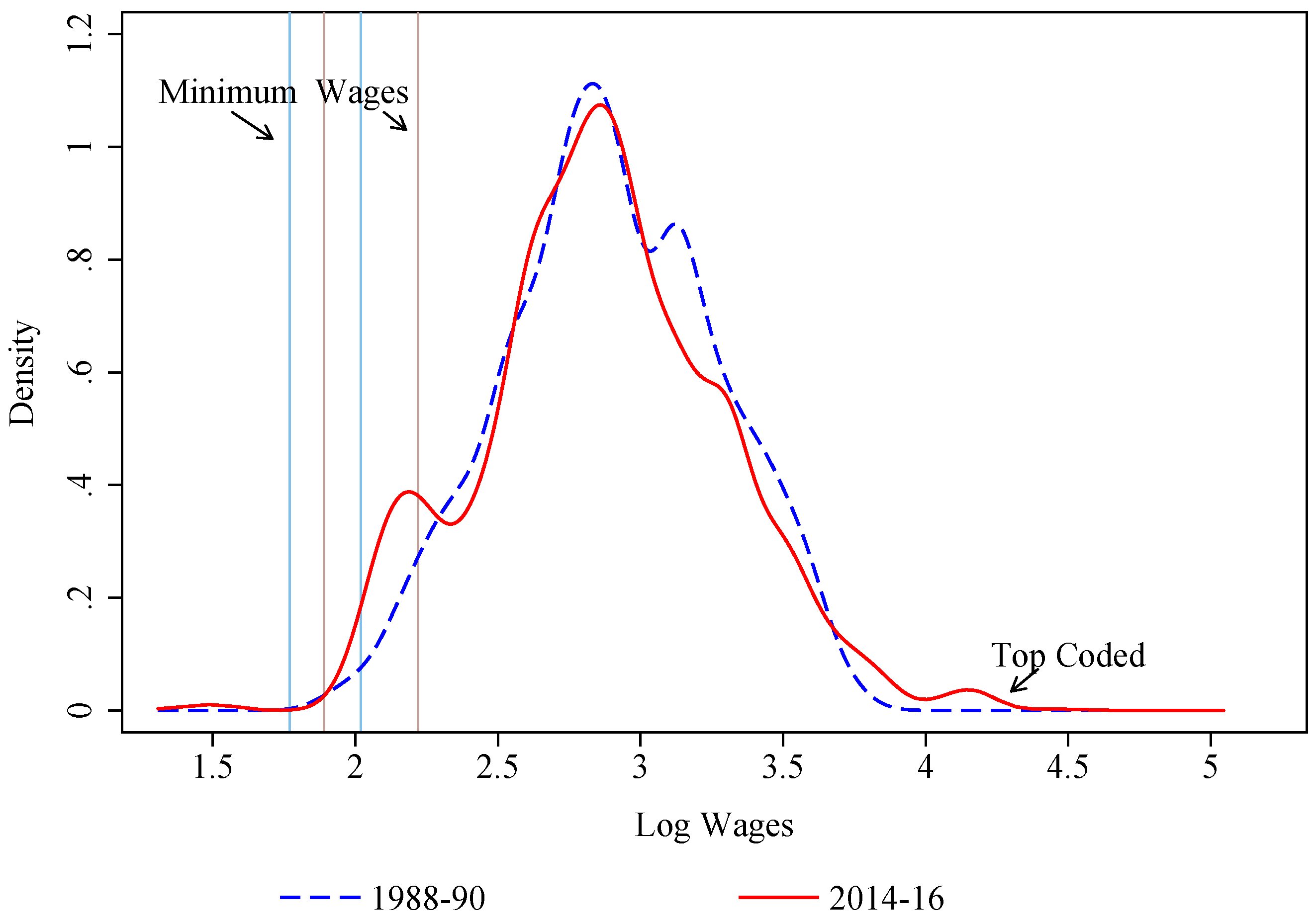
Before proceeding to the estimation of RIF-regressions, it is important to inspect the density of wages for unusual features that would challenge the estimation of the RIF at the quantiles of interest or the wage model that w use. Figure 1 presents kernel density estimates of male wages for 1988–1990 and 2014–2016 estimated using the Epanechnikov kernel and bandwidths of 0.06 and 0.08, respectively.22 The figure also shows the 1988–1990 density reweighted to have the same distribution of characteristics as in 2014–2016. The typical issues to look for include cliffs associated with minimum wage effects at the bottom of the distribution, peaks associated with heaping (the fact that hourly wage workers, in particular, are more likely to round their wages at next dollar amount) in the middle of the distribution, and top-coding at the top of the distribution. The impact of minimum wages is clearly seen in Figure 1 when vertical lines corresponding to the minimum and maximum of federal and state minimum wages are displayed. Because we do not model minimum wages in the current paper, the 1988–1990 density and the reweighted density are superimposed in those wage ranges, showing the wage setting variables that we include are inadequate for modeling the distribution of wages when minimum wages matter.23 Thus, we remain cautious with regards to the interpretation of any effect at the bottom of the distribution.
Heaping and top-coding can be problematic if they imply an unusually high value of the density at a particular quantile of interest that potentially biases the estimation of the denominator of the influence function (14). While only 0.7% of workers are top-coded in 1988–1990, this proportion increases to 3.6% in 2014–2016.24 A standard adjustment for top-coding consists of multiplying top-coded wages by a fixed adjustment factor. In Figure 1, we use the adjustment factor of 1.4 suggested by Lemieux (2006b). While there is no visual evidence of an impact of top-coding in 1988–1990, there is a clear spike in the 2014–2016 distribution around the point (log wage of about 4.5) where most top-coded observations lie.25 We deal with this issue using a more sophisticated stochastic imputation procedure (shown as the solid line) based on a Pareto distribution estimated using tax data from Alvaredo et al. (2013).
Given our large sample of hourly paid and salaried workers, heaping does not appear to be a serious issue in Figure 1.26 However, heaping is more visible in Figure 2, which plots the 1988–1990 and 2014–2016 densities of wages for our base group. This group of about 400 workers in each period consists of non-unionized, white, married, high school educated men with 20 to 25 years of experience, working as construction workers in the construction industry, but not in the public sector.27 The figure shows that the densities have changed very little over time, aside from different positioning of some local peaks associated with heaping.28 This group was chosen because the economic forces that impact the overall wage distribution are less likely at play among this non-unionized group of low-educated workers in non-routine manual jobs with little exposure to international trade.29
5.1. RIF-Regressions
Before showing the decomposition results, we first present some estimates from the RIF-regressions for different wage quantiles, the variance of log wages, and the Gini coefficient. From Equation (14), we compute for each observation using the sample estimate of , and the kernel density estimate of .
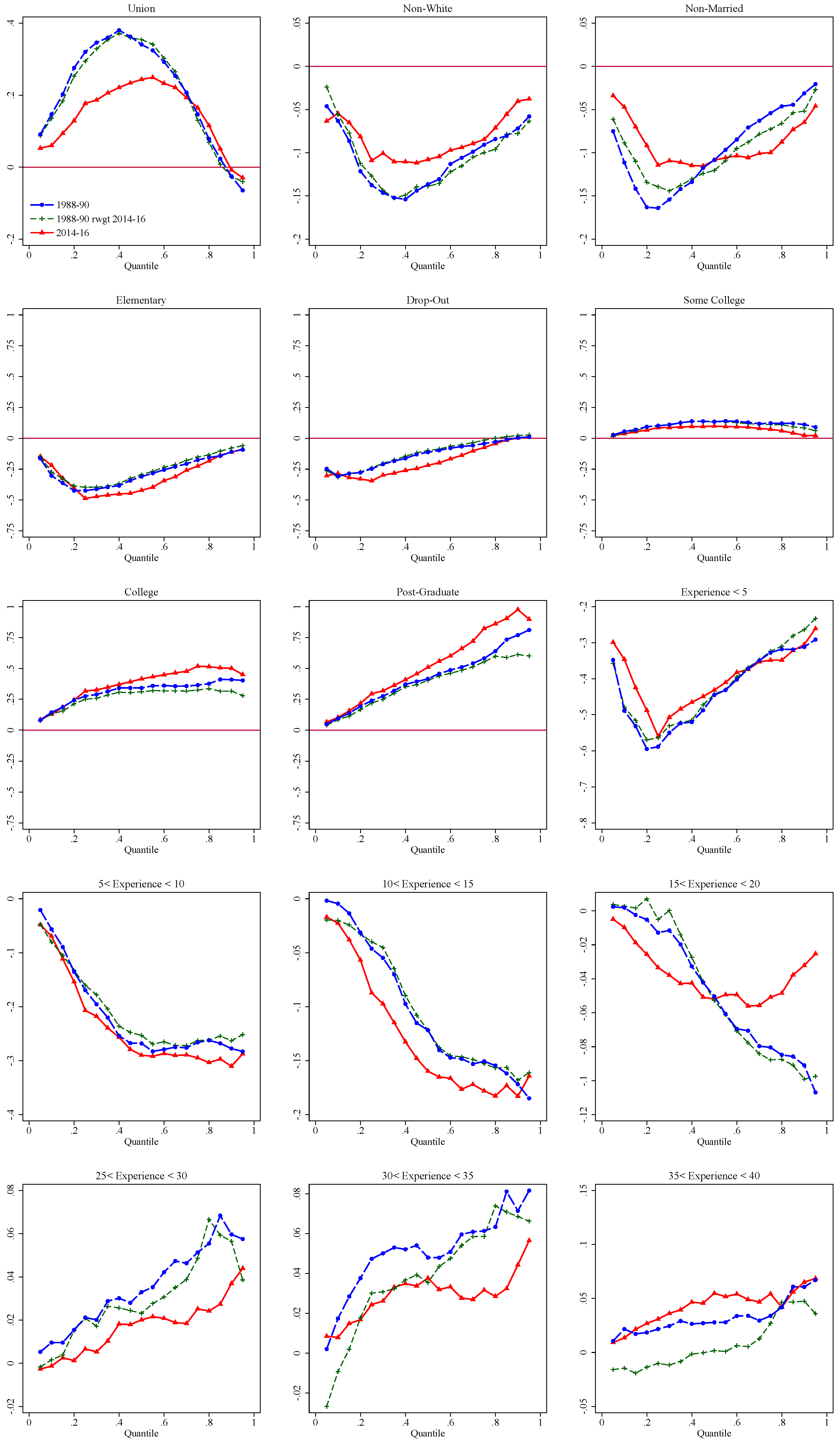
The RIF-regression coefficients for the 10th, 50th, and 90th quantiles in 1988–1990 and 2014–2016, along with bootstrapped standard errors, are reported in Table 1. The RIF-regression coefficients for the variance and the Gini are reported in Table 2. Detailed estimates for each of the 19 quantiles from the 5th to the 95th are also reported in Figure 3, Figure 4 and Figure 5. For several covariates (for example, union status, non-white, married, clerical, production, and service occupations, transportation and utility, public administration sectors). Figure 3 illustrates highly non-monotonic effects across the different quantiles for some demographics. For instance, in Panel 1, the effect of union status first increases up to around the 40th quantile in 1988–1990, and up the 50th quantile in 2014–2016, and then declines, even turning negative for the 90th and 95th quantiles.
As shown by the RIF-regressions for the more global measures of inequality—the variance of log wages and the Gini coefficient of the wage distribution—displayed in Table 2, the effect of unions on these measures is negative, although the magnitude of that effect has decreased over time. This is consistent with the well-known result (e.g., Freeman 1980) that unions tend to reduce the variance of log wages for men. More importantly, as shown in Table 1, the results also indicate that unions increase inequality in the lower end of the distribution, but decrease inequality even more in the higher end of the distribution. As we will see later in the decomposition results, this means that the continuing decline in the rate of unionization can account for some of the “polarization” of the labor market (decrease in inequality at the low-end, but increase in inequality at the top end). The results for unions also illustrate an important feature of RIF regressions for quantiles, namely that they capture both the between-group effect (arising from union wage premia) and the within-group effect (arising from wage union compression) of unions on wage dispersion, which go in opposite direction in this case.30
The RIF-regression estimates in Table 1 for other covariates also illustrate this point. Consider, for instance, the case of college education. Table 1 and Figure 3 show that the effect of college increases monotonically as a function of percentiles. In other words, increasing the fraction of the workforce with a college degree has a larger impact on higher than lower quantiles. The reason why the effect is monotonic is that education increases both the level and the dispersion of wages (see, e.g., Lemieux 2006a). As a result, both the within- and the between-group effects go in the same direction of increasing inequality.
Another clear pattern that emerges in Figure 3 and Figure 4 is that for most inequality enhancing covariates, i.e., those with a positively sloped curve, the inequality enhancing effect increases over time. In particular, the slopes for high levels of education (college graduates and post-graduates) and high-wage occupations (upper management, engineers and computer scientists, doctors, and lawyers) become steeper over time. This suggests that these covariates make a positive contribution to the wage structure effect.
There are some changes in the contribution of occupations and industries that are consistent with technological change and the routine-biased polarization of wages. For example, as shown in Figure 4 and Figure 5, there are increases in the returns to high-tech service industries at the upper end of the wage distribution, but decreases in the returns to production and clerical occupations in the middle of the wage distribution. There are also decreases in the penalties to some low skilled non-routine occupations and associated industries, such as service occupations and truck driving and the retail industry, although some increases at the lower end appear to be driven by changes in minimum wages. On the other hand, there are some offsetting effects in industries that could have compensated the decline in manufacturing employment, such as the primary (e.g., mining), wholesale and retail trade, and personal services industries. In summary, the changes in the rewards and penalties associated with occupations and industries provide a descriptive account of factors potentially offsetting the wage effects of the polarization of employment. We turn next to the evaluation of the magnitude of these effects.
5.2. Decomposition Results
The results for the aggregate decomposition are presented in Figure 6. Table 3 and Table 4 summarize the results for the standard measures of top-end (90–50 log wage differential) and low-end (50–10 log wage differential) wage inequality, as well as for the variance of log wages and the Gini coefficient. The covariates used in the RIF-regression models are those discussed above and listed in Table A1. A richer specification with additional interaction terms is used to estimate the logit models used compute the reweighting factor .31
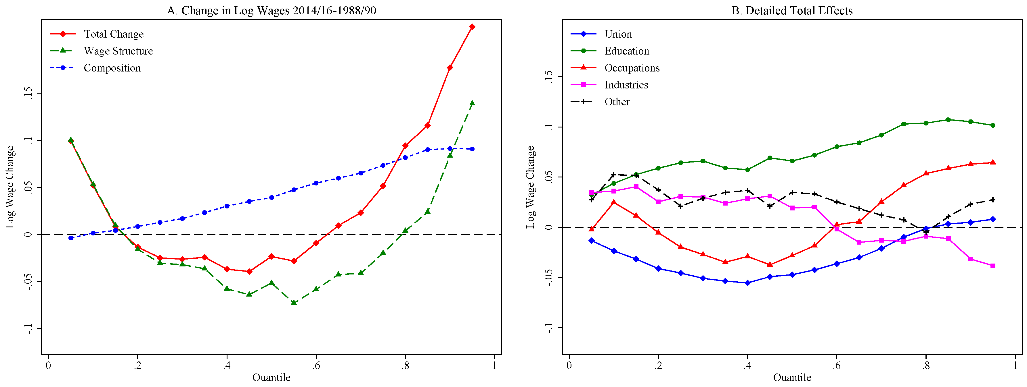
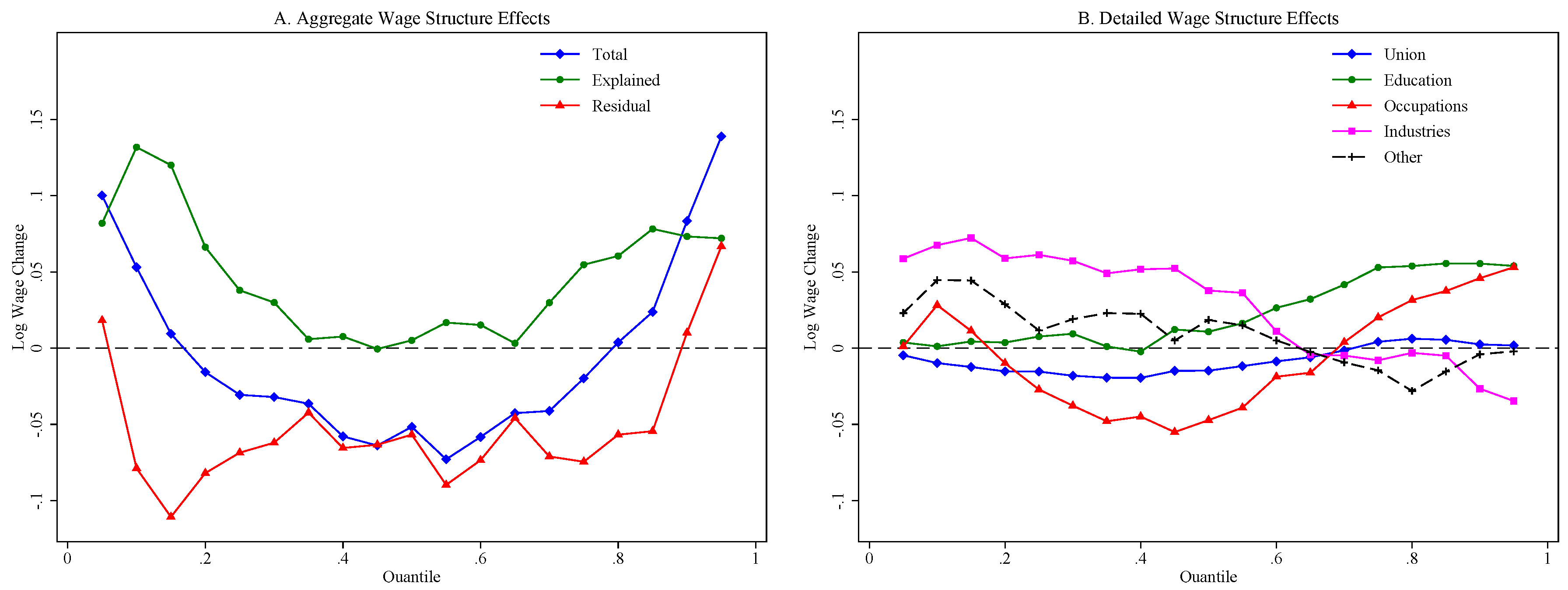
Figure 6a shows the overall change in (real log) wages at each percentile , , and decomposes this overall change into a composition () and wage structure () effect computed using the reweighting procedure of Result 1. Consistent with the pattern first documented in Autor et al. (2006), the overall change is U-shaped as wage dispersion increases in the top-end of the distribution, but declines in the lower end.32 Most summary measures of inequality such as the 90–10 gap nonetheless increase over the 1988–1990 to 2014–2016 period as wage gains in the top-end of the distribution exceed those at the low-end. In other words, although the curve for overall wage changes is U-shaped, its slope is positive, on average, suggesting that inequality generally goes up. This overall increase shows up as positive total changes in the 90–10 gap, the variance of log wages, and the Gini, reported in Table 3 and Table 4. In all cases, the aggregate decomposition of these overall measures attributes most (from 55% to 66%) of the changes to composition effects.
Figure 6a also shows that, consistent with Lemieux (2006b), composition effects have contributed to a substantial increase in inequality. In fact, once composition effects are accounted for, the remaining wage structure effects (estimated using reweighting) follow a “purer” U-shape than overall changes in wages. The wage declines are now right in the middle of the distribution (20th to 80th percentile), while wage gains at the top and low end are more similar. By the same token, however, composition effects cannot account at all for the U-shaped nature of wage changes.
Figure 7 moves to the next step of the decomposition using linear RIF-regressions to attribute the contribution of each set of covariates to the composition effect.33 Figure 8, which we discuss below, does the same for the wage structure effect. Figure 6b summarizes the total of the composition and wage structure effects by the sets of factors of interest. The combination of composition and wage structure effects shows the strong monotonic effect of education on wage changes, the mild U-shaped effect of union and occupations, and the offsetting hump-shaped effect of industries.
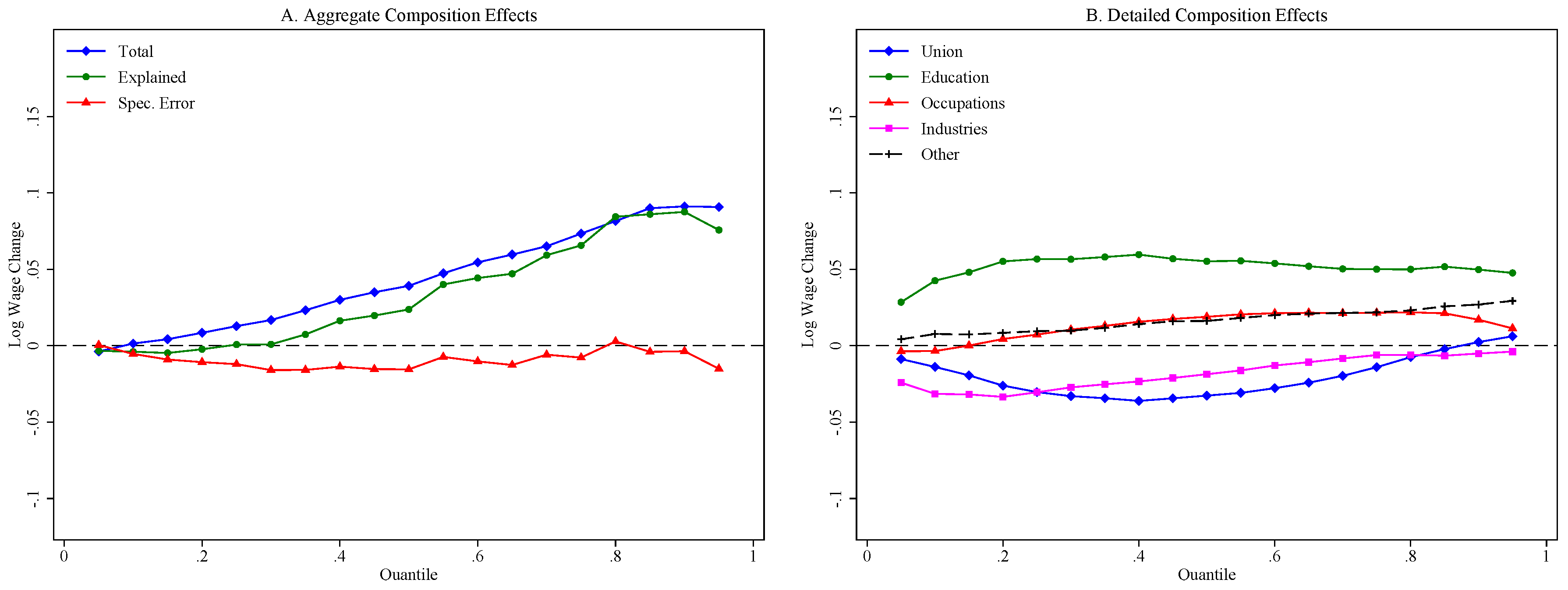
Figure 7a compares the overall composition effect obtained by reweighting and displayed in Figure 6a, , to the composition effect explained using the RIF-regressions, . The difference between the two curves is the specification (approximation) error . The error term is relatively small and does not exhibit much of a systematic pattern. This means that the RIF-regression model does relatively well at tracking down the composition effect estimated consistently using the reweighting procedure; however, as we discuss below, in some cases, the specification error is significantly different from zero.
Figure 7b then divides the composition effect (explained by the RIF-regressions) into the contribution of five main sets of factors. To simplify the discussion, we focus on the impact of each factor on overall wage inequality summarized by the 90–10 log wage differential in comparison to the 50–10 and 90–50 log wage differentials that capture what happened in the lower and upper parts of the distribution, respectively. The decomposition of the log wage differentials, the log variance, and the Gini are reported in Table 3 and Table 4. Table 3 presents the simple OB type decomposition computed from RIF-regressions of the five inequality measures, without reweighting. Table 4 applies the complete two-step procedure described above.
As discussed in Section 4.3, we compute the RIF of the difference between two (log) quantiles and , where , as , and use these differences as dependent variables in the regressions. For the variance of log wages and the Gini, the RIF are as described above. Using the estimation results from these sets of regressions, we compute the components of the simple OB-type decomposition for the changes over time, , from 1988–1990 () to 2014–2016 () as:
These results are displayed in Table 3 by groups of variables.34 In Table 4, we present the results of the decomposition that also applies the reweighting procedure
The four terms in this decomposition are easily obtained by running two OB decompositions using RIF regressions. First, we perform an OB decomposition using the sample and the counterfactual sample ( sample reweighted to be as in ) to get the pure composition effect, , using as reference wage structure. The total unexplained effect in this decomposition corresponds to the specification error, , and allows one to assess the importance of departures from the linearity assumption. Second, we perform the decomposition using the sample and the counterfactual sample, using the counterfactual wage structure as reference, and obtain the pure wage structure effect, , in the “unexplained" part of the decomposition. The total explained effect in this decomposition, , corresponds to the reweighting error which should go to zero in large samples. It provides an easy way of assessing the quality of the reweighting.35
Consistent with Figure 7a, specification errors reported in Table 4 are generally small. As discussed in Section 3, the specification error reflects departures from non-linearity of the RIF-regressions and the fact that, except for the mean, the RIF depends on the distribution of Y (and X through its effect on Y). In Table 4, we formally test whether the specification error is significantly different from zero. The results are mixed. The specification error is not significantly different from zero for the 90–10 and the 50–10 gaps, but is statistically significant for the 90–50 gap, the variance, and the Gini. The specification error is nonetheless small relative to the overall changes in the distributional statistics, which indicates that RIF-regressions provide highly accurate estimates of the overall composition and wage structure effects in the empirical example being studied here. However, as we discuss below, although the specification error is small, using the two-step decomposition instead of a standard OB decomposition matters much more when looking at the contribution of individual covariates to the wage structure effect.
In both Table 3 and Table 4, the composition effects linked to factors other than unions go the “wrong way” in the sense that they account for rising inequality at the bottom end while inequality is rising at the top end, a point noted earlier by Autor et al. (2005). This applies in particular to education and occupations effects that are larger for the 50–10 than for the 90–50, while the effects of industry and other factors (race, marital status, and experience) on the 50–10 and 90–50 are similar. In contrast, composition effects linked to unions (the impact of de-unionization) reduce inequality at the low end (effect of −0.019 on the 50–10) but increases inequality at the top end (effect of 0.035 on the 90–50). Note that, just as in an OB decomposition, these effects on the 50–10 and the 90–50 gap can be obtained directly by multiplying the 9.5 percent decline in the unionization rate (Table A1) by the relevant union effects in 1988–1990 shown in Table 1. The effect of de-unionization accounts for about 25 percent of the total change in the 50–10 gap, which is remarkably similar to the relative contribution of de-unionization to the growth in inequality in the 1980s (see Freeman 1993; Card 1992; and DiNardo et al. 1996).
Figure 8a divides the wage structure effect, , into the part explained by the RIF-regression models, , and the residual change (the change in for the base group captured by the intercepts). The contribution of each set of factors is then shown in Figure 8b. As in the case of the composition effects, it is easier to discuss the results by focusing on the 90–50 and 50–10 gaps shown in Table 3 and Table 4.
Here, we note that the contribution of different covariates to the wage structure effect are quite different in Table 3 and Table 4. This indicates that the OB decomposition of Table 3 is inaccurate because of differences between the estimated RIF-regression coefficients and . As discussed in Section 3, the difference between and used to compute wage structure effects in Table 4 solely reflects changes in the wage structure. By contrast, the difference between and used in Table 3 is likely contaminated by changes in the distribution of X that are being adjusted for (by reweighting) when estimating . The difference is particularly striking in the case of education. As expected, Table 4 shows that wages structure effects linked to education play an important role in the growth of the 90–50 gap. By contrast, the effect is small and insignificant when using a conventional OB decomposition in Table 3. The case of education, a central variable in most studies on the sources of growing inequality, dramatically illustrates the importance of using the two-step decomposition with reweighting proposed in this paper.
The wage structure results of Table 4 first show that covariates overexplain −0.127 (sum of the five effects) of the −0.105 change (decline) in the 50–10 gap, the constant capturing the difference. Covariates do a less impressive job explaining changes in the 90–50 gap explaining only 0.068 (half) of the 0.136 change. Occupations are the set of the covariates that best capture the changes in the wage structure. They account for −0.075 of the −0.105 decline (73%) in the 50–10 gap and 0.088 of the 0.135 increase (68%) in the 90–50 gap. These results justify the increased attention given in the literature to the role of occupational tasks (Firpo et al. 2011; Fortin and Lemieux 2016). Changes in the returns to education continue to play an important role at the top of distribution accounting for 0.045 of the 0.135 increase (33%) in the 90–50. This supports Lemieux (2006a)’s conjecture that increases in the return to post-secondary education contribute to the convexification of the wage distribution.
Finally, the total effect of each covariate (wage structure plus composition effect) is reported in Figure 6b and the bottom panel of Table 4. Unions and occupations are the two factors that best account for the differential changes at the bottom and top of the distribution, capturing both a negative effect on the 50–10 and a positive effect on the 90–50. The total effect of the two factors on the 50–10 gap corresponds to −0.078 out of −0.105 (74%) of the change, while they account for 0.139 out of 0.136 change in the 90–50 (102%). This goes a substantial way towards explaining the polarization of the labor market.
6. Conclusions
We provide a detailed exposition of a two-stage method to decompose changes in the distribution of wages (or other outcome variables). In Stage 1, distributional changes are divided into a wage structure effect and a composition effect using a reweighting method. In Stage 2, these two components are further divided into the contribution of each individual covariate using the recentered influence function regression technique introduced by FFL. This two-stage procedure generalizes the popular OB decomposition method by extending the decomposition to any distributional measure (besides the mean), and allowing for a more flexible wage setting model. Other procedures (Machado and Mata 2005; Melly 2005; Rothe 2012; CFM) have been suggested for performing part of this decomposition for distributional parameters besides the means. One important advantage of our procedure is that it is easy to use in practice, as it simply involves estimating a logit model (first stage) and running least-square regressions (second stage). Another more distinctive advantage is that it can be used to divide the contribution of each covariate to the composition effect, something that most existing methods cannot do.
We illustrate the workings of our method by looking at changes in male wage inequality in the United States between 1988 and 2016. This is an interesting case to study as the wage distribution changed very differently at different points of the distribution, a phenomenon that cannot be captured by summary measures of inequality such as the variance of log wages. Our method is particularly well suited for looking in detail at the source of wage changes at each percentile of the wage distribution. Our findings indicate that unions, occupations, and education are the most important factors accounting for the observed changes in the wage distribution over this period.
Author Contributions
All authors contributed equally to the paper.
Funding
Fortin and Lemieux thank the Social Sciences and Humanities Research Council of Canada (grant# for financial support. Firpo thanks CNPq-Brazil for financial support.
Conflicts of Interest
The authors declare no conflict of interest.
Appendix A. Tables

Table A1.
Sample Means.
| Years: | 1988/90 | 2014/16 | Difference |
|---|---|---|---|
| Log wages | 2.860 | 2.901 | 0.041 |
| Std of log wages | 0.579 | 0.622 | 0.043 |
| Union covered | 0.223 | 0.127 | −0.095 |
| Non-white | 0.134 | 0.186 | 0.052 |
| Non-Married | 0.388 | 0.457 | 0.068 |
| Age | 36.204 | 39.882 | 3.677 |
| Education | |||
| Primary | 0.059 | 0.034 | −0.025 |
| Some HS | 0.118 | 0.054 | −0.064 |
| High School | 0.381 | 0.307 | −0.074 |
| Some College | 0.202 | 0.275 | 0.072 |
| College | 0.139 | 0.218 | 0.078 |
| Post-grad | 0.101 | 0.113 | 0.012 |
| Occupations | |||
| Upper Management | 0.082 | 0.080 | −0.002 |
| Lower Management | 0.040 | 0.068 | 0.028 |
| Engineers & Computer Occ. | 0.061 | 0.081 | 0.019 |
| Other Scientists | 0.014 | 0.010 | −0.004 |
| Social Support Occ. | 0.052 | 0.061 | 0.009 |
| Lawyers & Doctors | 0.010 | 0.015 | 0.005 |
| Health Treatment Occ. | 0.010 | 0.019 | 0.009 |
| Clerical Occ. | 0.066 | 0.068 | 0.002 |
| Sales Occ. | 0.086 | 0.085 | −0.001 |
| Insur. & Real Estate Sales | 0.007 | 0.006 | −0.001 |
| Financial Sales | 0.003 | 0.002 | −0.001 |
| Service Occ. | 0.107 | 0.149 | 0.042 |
| Primary Occ. | 0.026 | 0.011 | −0.015 |
| Construction & Repair Occ. | 0.164 | 0.155 | −0.009 |
| Production Occ. | 0.141 | 0.086 | −0.055 |
| Transportation Occ. | 0.086 | 0.060 | −0.026 |
| Truckers | 0.045 | 0.041 | −0.004 |
| Industries | |||
| Agriculture, Mining | 0.033 | 0.026 | −0.007 |
| Construction | 0.097 | 0.101 | 0.005 |
| Hi-Tech Manufac | 0.102 | 0.066 | −0.037 |
| Low-Tech Manufac | 0.137 | 0.087 | −0.050 |
| Wholesale Trade | 0.051 | 0.033 | −0.018 |
| Retail Trade | 0.105 | 0.113 | 0.008 |
| Transportation & Utilities | 0.086 | 0.079 | −0.008 |
| Information except Hi-Tech | 0.018 | 0.012 | −0.006 |
| Financial Activities | 0.047 | 0.058 | 0.011 |
| Hi-Tech Services | 0.035 | 0.064 | 0.029 |
| Business Services | 0.051 | 0.065 | 0.014 |
| Education & Health Services | 0.097 | 0.113 | 0.016 |
| Personal Services | 0.081 | 0.127 | 0.046 |
| Public Admin | 0.058 | 0.054 | −0.005 |
| Public Sector | 0.149 | 0.126 | −0.024 |
Note: Computed using sample weights. All differences over time are statistically significant at the p = 0.001 level.
Table A2.
Occupation and Industry Definitions.
| Code Sources: | 2010 Census SOC | 1980 SOC |
|---|---|---|
| Occupations | ||
| Upper Management | 10–200, 430 | 1–13, 19 |
| Lower Management | 200–950 | 14–18, 20–37, 473–476 |
| Engineers & Computer Occ. | 1000–1560 | 43–68, 213–218, 229 |
| Other Scientists | 1600–1960 | 69–83, 166–173, 223–225, 235 |
| Social Support Occ. | 2000–2060, 2140–2960 | 113–165, 174–177, 183–199, 228, 234 |
| Lawyers & Doctors | 2100–2110, 3010, 3060 | 84–85, 178–179 |
| Health Treatment Occ. | 3000, 3030–3050, 3110–3540 | 86–106, 203–208 |
| Clerical Occ. | 5000–5940 | 303–389 |
| Sales Occ. | 4700–4800, 4830–4900, 4930–4965 | 243–252, 256–285 |
| Insur. & Real Estate Sales | 4810,4920 | 253–254 |
| Financial Sales | 4820 | 255 |
| Service Occ. | 3600–4650 | 430–470 |
| Primary Occ. | 6000–6130 | 477–499 |
| Construction & Repair Occ. | 6200–7620 | 503–617, 863–869 |
| Production Occ. | 7700–8960 | 633–799, 873, 233 |
| Transportation Occ. | 9000–9120, 9140–9750 | 803, 808–859, 876–889, 226–227 |
| Truck Drivers | 9130 | 804–806 |
| Industries | ||
| Agriculture, Mining | 170–490 | 10–50 |
| Construction | 770 | 60 |
| Hi-Tech Manufac | 2170–2390, 3180, 3360–3690, 3960 | 180–192, 210–212, 310, 321–322, 340–372 |
| Low-Tech Manufac | 1070–2090, 2470–3170, 3190–3290, 3770–3890, 3970–3990 | 100–162, 200–201,220–301, 311–320, 331–332, 380–392 |
| Wholesale Trade | 4070–4590 | 500–571 |
| Retail Trade | 4670–5790 | 580–640, 642–691 |
| Transportation & Utilities | 570–690, 6070–6390 | 400–432, 460–472 |
| Information except Hi-Tech | 6470–6480, 6570–6670, 6770–6780 | 171–172, 852 |
| Financial Activities | 6870–7190 | 700–712 |
| Hi-Tech Services | 6490, 6675–6695, 7290–7460 | 440–442, 732–740, 882 |
| Business Services | 7270–7280, 7470–7790 | 721–731, 741–791, 890, 892 |
| Education & Health Services | 7860–8470 | 812–851, 860–872, 891 |
| Personal Services | 8560–9290 | 641, 750–802, 880–881 |
| Public Admin | 9370–9590 | 900–932 |
Appendix B. Supplemental Material
Appendix B.1. Details of Weighting Functions Estimation
Appendix B.1.1. Estimating the Weights
We are interested in estimating weights that are generally functions of the distribution of (). The three weighting functions under consideration are , , and . The first two weights are trivially estimated as:
where .
The weighting function can be estimated as
where is an estimator of the true probability of being in Group 1 given X. We describe in detail below the two approaches that we consider, a parametric one and a non-parametric one. In addition, to have weights summing up to one, we use the following normalization procedures:
Appendix B.1.2. Estimating the Distributional Statistics
We are interested in the estimation and inference of , , and . It can be shown that, under certain regularity conditions, estimators of these objects will be distributed asymptotically normal. We now show how to estimate those quantities, and derive their asymptotic distributions below.
The estimation follows a plug-in approach. Replacing the CDF by the empirical distribution function yields the estimators of interest:
where
Note that, in practice, it is not usually necessary to compute these empirical distribution functions to get estimates of a distributional statistic, . Standard software programs such as Stata can be used to compute distributional statistics directly from the observations on Y using the appropriate weighting factor.
The estimated distributional statistics can then be used to estimate the wage structure and composition effects as and .
Appendix B.1.3. Parametric Propensity Score Estimation
Suppose that is correctly specified up to a finite vector of parameters . That is, or more formally:
Assumption A1.
(Parametric p-score) ; where is a known function up to , .
Estimation of follows by maximum likelihood:
Define the derivative of with respect to as . The score function is:
Using a normalization argument, we suppress the entry for whenever a function of it is evaluated at the true . Therefore,
and finally
In particular, in this paper, we assume that the can be modeled as a logit, that is,
where ,.
Appendix B.1.4. Nonparametric Propensity Score Estimation
Suppose that is completely unknown to the researcher. In that case, following Hirano et al. (2003), we approximate the log odds ratio by a polynomial series. In practice, this is done by finding a vector that is the solution of the following problem:
where , a vector of length J of polynomial functions of satisfying the following properties: (i) ; and () . More details on this estimation procedure can be found at Hirano et al. (2003) or in Firpo (2007). The non-parametric feature of this estimation procedure comes from the fact that such approximation is refined as the sample size increases, that is, J will be a function of the sample size as .
In this approach, is estimated by , thus:
Appendix B.2. Asymptotic Distribution
We first show that the plug-in estimators are asymptotically normal and compute their asymptotic variances. We then do the same for the density estimators.
Appendix B.2.1. The Asymptotic Distribution of Plug-In Estimators
We start by assuming that the estimators are asymptotically linear in the following sense:
Assumption A2 (Asymptotic Linearity).
and are asymptotically linear, that is,
Assumption A2 establishes that the estimators are either exactly linear, as those that are based on sample moments, or they can be linearized and the remainder term will approach zero as the sample size increases.
An additional technical assumption is that the influence function are square integrable and its conditional expectation given X is differentiable. To simplify notation, let us write .
Assumption A3.
For all weighting functions ω considered,
(i) , and
(ii) and are continuously differentiable for all x in .
Under ignorability, both types of estimators (parametric and non-parametric first step) for , , and proposed before will remain asymptotically linear. The theorem below considers both the parametric and non-parametric cases.
Theorem A1.
:
Under Assumptions 1, 2, A2 and A3:
(i-ii) ,
(iii) (a) if in addition, Assumption A1 holds, then:
(iii) (b) otherwise, if in addition we assume [non-parametric], then:
where
Appendix B.3. Proofs
Proof of Result 1.
A proof can be found in Firpo and Pinto (2016). □
Proof of Result 2.
Part (i) is straightforward and follows from identification of the functionals , and , a direct consequence of identification of , and . Part () follows from the fact that
where
thus, if , then for all y, and
Part () follows from a similar argument:
where
thus if , then for all x, and therefore, for all y, and
□
Proof of Theorem A1.
A proof of parts (i), () and () (b) can be found in Firpo and Pinto (2016). A proof of part () (a) can be found in Chen et al. (2008). □
References
- Acemoglu, Daron, and David H. Autor. 2011. Skills, Tasks, and Technologies: Implications for Employment and Earnings. In Handbook of Labor Economics. Edited by Orley Ashenfelter and David Card. Amsterdam: North-Holland, vol. IV.B, pp. 1043–172. [Google Scholar]
- Alvaredo, Facundo, Anthony B. Atkinson, Thomas Piketty, and Emmanuel Saez. 2013. The Top 1 Percent in International and Historical Perspective. Journal of Economic Perspectives 27: 3–20. [Google Scholar] [CrossRef]
- Autor, David H., and David Dorn. 2013. The Growth of Low-Skill Service Jobs and the Polarization of the US Labor Market. American Economic Review 103: 1553–97. [Google Scholar] [CrossRef] [Green Version]
- Autor, David H., David Dorn, Gordon H. Hanson, and Jae Song. 2014. Trade Adjustment: Worker-level Evidence. Quarterly Journal of Economics 129: 1799–860. [Google Scholar] [CrossRef]
- Autor, David H., David Dorn, and Gordon H. Hanson. 2015. Untangling Trade and Technology: Evidence from Local Labour Markets. Economic Journal 125: 621–46. [Google Scholar] [CrossRef]
- Autor, David H., Lawrence F. Katz, and Melissa S. Kearney. 2005. Rising Wage Inequality: The Role of Composition and Prices. NBER Working paper No. 11628. Cambridge, MA, USA: National Bureau of Economic Research. [Google Scholar]
- Autor, David H., Lawrence F. Katz, and Melissa S. Kearney. 2006. The Polarization of the U.S. Labor Market. American Economic Review 96: 189–94. [Google Scholar] [CrossRef]
- Autor, David H., Frank Levy, and Richard J. Murnane. 2003. The Skill Content Of Recent Technological Change: An Empirical Exploration. Quarterly Journal of Economics 118: 1279–333. [Google Scholar] [CrossRef]
- Barsky, Robert, John Bound, Kerwin Kofi Charles, and Joseph P. Lupton. 2002. Accounting for the Black-White Wealth Gap: A Nonparametric Approach. Journal of the American Statistical Association 97: 663–73. [Google Scholar] [CrossRef]
- Bento, Antonio, Kenneth Gillingham, and Kevin Roth. 2017. The Effect of Fuel Economy Standards on Vehicle Weight Dispersion and Accident Fatalitiesc. NBER Working paper No. w23340. Cambridge, MA, USA: National Bureau of Economic Research. [Google Scholar]
- Blinder, Alan. 1973. Wage Discrimination: Reduced Form and Structural Estimates. Journal of Human Resources 8: 436–55. [Google Scholar] [CrossRef]
- Brochu, Pierre, David A. Green, Thomas Lemieux, and James Townsend. 2017. The Minimum Wage, Turnover, and the Shape Effects of Wage Distribution. In Mimeo. Vancouver: University of British Columbia. [Google Scholar]
- Card, David. 1992. The Effects of Unions on the Distribution of Wages: Redistribution or Relabelling? NBER Working paper No. 4195. Cambridge, MA, USA: National Bureau of Economic Research. [Google Scholar]
- Cattaneo, Matias D., Michael Jansson, and Xinwei Ma. 2017. Simple Local Polynomial Density Estimators. In Mimeo. Berkeley: UC Berkeley. [Google Scholar]
- Chamberlain, Gary. 1994. Quantile Regression Censoring and the Structure of Wages. In Advances in Econometrics. Edited by Christopher Sims. New York: Elsevier. [Google Scholar]
- Chernozhukov, Victor, Ivan Fernandez-Val, and Blaise Melly. 2013. Inference on Counterfactual Distributions. Econometrica 81: 2205–68. [Google Scholar]
- Chen, Xiaohong, Han Hong, and Alessandro Tarozzi. 2008. Semiparametric Efficiency in GMM Models with Auxiliary Data. The Annals of Statistics 36: 808–43. [Google Scholar] [CrossRef]
- Choe, Chung, and Philippe Van Kerm. 2014. Foreign Workers and the Wage Distribution: Where Do They Fit in? Technical Report 2014-02. Esch-sur-Alzette: Luxembourg Institute of Socio-Economic Research. [Google Scholar]
- Cowell, Frank, and Maria-Pia Victoria-Feser. 1996. Robustness Properties of Inequality Measures. Econometrica 64: 77–101. [Google Scholar] [CrossRef]
- DiNardo, John, Nicole M. Fortin, and Thomas Lemieux. 1996. Labor Market Institutions and the Distribution of Wages, 1973–1992: A Semiparametric Approach. Econometrica 64: 1001–44. [Google Scholar] [CrossRef]
- Eeckhout, Jan, Roberto Pinheiro, and Kurt Schmidheiny. 2014. Spatial sorting. Journal of Political Economy 122: 554–620. [Google Scholar] [CrossRef]
- Essama-Nssah, Boniface, and Peter J. Lambert. 2012. Influence functions for policy impact analysis. In Inequality, Mobility and Segregation: Essays in Honor of Jacques Silber. Edited by John A. Bishop and Rafael Salas. Cheltenham: Emerald Group Publishing Limited, chp. 6. pp. 135–59. [Google Scholar]
- Firpo, Sergio. 2007. Efficient Semiparametric Estimation of Quantile Treatment Effects. Econometrica 75: 259–76. [Google Scholar] [CrossRef]
- Firpo, Sergio, Nicole M. Fortin, and Thomas Lemieux. 2007. Decomposing Wage Distributions using Recentered Influence Functions Regressions. In Mimeo. Vancouver: University of British Columbia. [Google Scholar]
- Firpo, Sergio, Nicole M. Fortin, and Thomas Lemieux. 2009. Unconditional Quantile Regressions. Econometrica 77: 953–973. [Google Scholar]
- Firpo, Sergio, Nicole M. Fortin, and Thomas Lemieux. 2011. Occupational Tasks and Changes in the Wage Structure. In Mimeo. Vancouver: University of British Columbia. [Google Scholar]
- Firpo, Sergio, and Cristine Pinto. 2016. Identification and Estimation of Distributional Impacts of Interventions Using Changes in Inequality Measures. Journal of Applied Econometrics 31: 457–86. [Google Scholar] [CrossRef]
- Fortin, Nicole, Thomas Lemieux, and Sergio Firpo. 2011. Decomposition Methods in Economics. In Handbook of Labor Economics. Edited by Orley Ashenfelter and David Card. Amsterdam: North-Holland, vol. IV.A, pp. 1–102. [Google Scholar]
- Fortin, Nicole, and Thomas Lemieux. 2016. Inequality and Changes in Task Prices: Within and between Occupation Effects? In Income Inequality, Causes and Consequences (Research in Labor Economics, Vol. 43). Edited by Lorenzo Cappellari, Solomon W. Polachek and Konstantinos Tatsiramos. Cheltenham: Emerald Group Publishing Limited, pp. 195–226. [Google Scholar]
- Freeman, Richard B. 1980. Unionism and the Dispersion of Wages. Industrial and Labor Relations Review 34: 3–23. [Google Scholar] [CrossRef]
- Freeman, Richard B. 1993. How Much has Deunionization Contributed to the Rise of Male Earnings Inequality? In Uneven Tides: Rising Income Inequality in America. Edited by Sheldon Danziger and Peter Gottschalk. New York: Russell Sage Foundation, pp. 133–63. [Google Scholar]
- Gâteaux, René. 1913. Sur les fonctionnelles continues et les fonctionnelles analytiques. Comptes Rendus de l’Académie des Sciences-Series I—Mathematics 157: 325–27. [Google Scholar]
- Gardeazabal, Javier, and Arantza Ugidos. 2004. More on the Identification in Detailed Wage Decompositions. Review of Economics and Statistics 86: 1034–57. [Google Scholar] [CrossRef]
- Gradín, Carlos. 2016. Why Is Income inequality so High in Spain? In Income Inequality Around the World (Research in Labor Economics, Vol. 44). Edited by Lorenzo Cappellari, Solomon W. Polachek and Konstantinos Tatsiramos. Cheltenham: Emerald Group Publishing Limited, pp. 109–77. [Google Scholar]
- Hampel, Frank R. 1974. The Influence Curve and Its Role in Robust Estimation. Journal of the American Statistical Association 60: 383–93. [Google Scholar] [CrossRef]
- Heckman, James J. 1990. Varieties of Selection Bias. American Economic Review 80: 313–18. [Google Scholar]
- Heckman, James J., Hidehiko Ichimura, and Petra Todd. 1997. Matching as an Econometric Evaluation Estimator. Review of Economic Studies 65: 261–94. [Google Scholar] [CrossRef]
- Heckman, James J., Hidehiko Ichimura, Jeffrey A. Smith, and Petra Todd. 1998. Characterizing Selection Bias Using Experimental Data. Econometrica 66: 1017–98. [Google Scholar] [CrossRef]
- Heckman, James J., and Richard Robb. 1985. Alternative Methods for Evaluating the Impact of Interventions: An Overview. Journal of Econometrics 30: 239–67. [Google Scholar] [CrossRef]
- Heckman, James J., and Richard Robb. 1986. Alternative Methods for Solving the Problem of Selection Bias in Evaluating the Impact of Treatments on Outcomes. In Drawing Inference from Self-Selected Samples. Edited by Howard Wainer. New York: Springer, pp. 63–107. [Google Scholar]
- Hirano, Keisuke, Guido W. Imbens, and Geert Ridder. 2003. Efficient Estimation of Average Treatment Effects Using the Estimated Propensity Score. Econometrica 71: 1161–89. [Google Scholar] [CrossRef]
- Jann, Ben. 2008. The Oaxaca-Blinder Decomposition for Linear Regression Models. Stata Journal 8: 435–79. [Google Scholar]
- Juhn, Chinhui, Kevin Murphy, and Brooks Pierce. 1993. Wage Inequality and the Rise in Returns to Skill. Journal of Political Economy 101: 410–42. [Google Scholar] [CrossRef]
- Kline, Patrick. 2011. Oaxaca-Blinder as a Reweighting Estimator. American Economic Review 101: 532–37. [Google Scholar] [CrossRef]
- Koenker, Roger. 2005. Quantile Regression. Cambridge: Cambridge University Press. [Google Scholar]
- Koenker, Roger, and Gilbert Bassett Jr. 1978. Regression Quantiles. Econometrica 46: 33–50. [Google Scholar] [CrossRef]
- Lemieux, Thomas. 2002. Decomposing Changes in Wage Distributions: A Unified Approach. Canadian Journal of Economics 35: 646–88. [Google Scholar] [CrossRef]
- Lemieux, Thomas. 2006a. Post-secondary Education and Increasing Wage Inequality. American Economic Review 96: 195–99. [Google Scholar] [CrossRef]
- Lemieux, Thomas. 2006b. Increasing Residual Wage Inequality: Composition Effects, Noisy Data, or Rising Demand for Skill? American Economic Review 96: 461–98. [Google Scholar] [CrossRef]
- Lemieux, Thomas. 2008. The Changing Nature of Wage Inequality. Journal of Population Economics 21: 21–48. [Google Scholar] [CrossRef]
- Machado, José A. F., and José Mata. 2005. Counterfactual Decomposition of Changes in Wage Distributions Using Quantile Regression. Journal of Applied Econometrics 20: 445–65. [Google Scholar] [CrossRef]
- Melly, Blaise. 2005. Decomposition of Differences in Distribution Using Quantile Regression. Labour Economics 12: 577–1990. [Google Scholar] [CrossRef]
- Monti, Anna Clara. 1991. The Study of the Gini Concentration Ratio by Means of the Influence Function. Statistica 51: 561–77. [Google Scholar]
- Oaxaca, Ronald. 1973. Male-Female Wage Differentials in Urban Labor Markets. International Economic Review 14: 693–709. [Google Scholar] [CrossRef]
- Oaxaca, Ronald, and Michael R. Ransom. 1999. Identification in Detailed Wage Decompositions. Review of Economics and Statistics 81: 154–57. [Google Scholar] [CrossRef]
- Rosenbaum, Paul R., and Donald B. Rubin. 1983. The Central Role of the Propensity Score in Observational Studies for Causal Effects. Biometrika 70: 41–55. [Google Scholar] [CrossRef]
- Rosenbaum, Paul R., and Donald B. Rubin. 1984. Reducing Bias in Observational Studies Using Subclassification on the Propensity Score. Journal of the American Statistical Association 79: 516–24. [Google Scholar] [CrossRef]
- Rothe, Christoph. 2010. Nonparametric Estimation of Distributional Policy Effects. Journal of Econometrics 155: 56–70. [Google Scholar] [CrossRef]
- Rothe, Christoph. 2012. Partial Distributional Policy Effects. Econometrica 80: 2269–301. [Google Scholar]
- Rothe, Christoph. 2015. Decomposing the Composition Effect. Journal of Business Economics and Statistics 33: 323–37. [Google Scholar] [CrossRef]
- Von Mises, Richard. 1947. On the Asymptotic Distribution of Differentiable Statistical Functions. The Annals of Mathematical Statistics 18: 309–48. [Google Scholar] [CrossRef]
- White, Halbert. 1980. Using Least Squares to Approximate Unknown Regression Functions. International Economic Review 21: 149–70. [Google Scholar] [CrossRef]
- Yun, Myeong-Su. 2005. A simple Solution to the Identification Problem in Detailed Wage Decompositions. Economic Inquiry 43: 766–72. [Google Scholar] [CrossRef]
| 1 | Recentered influence functions have since been derived for a host of inequality measures by Essama-Nssah and Lambert (2012). |
| 2 | Eeckhout et al. (2014) compare the CFM approach to the RIF-regressions approach to decompose the skill distributions across large and small cities in terms of education, occupations, and industries, focusing on the bottom and top decile. Bento et al. (2017) provide a useful comparison of local kernel regressions, conditional quantile regressions, and RIF regressions in the context of a Monte-Carlo simulation of the effect of fuel economy standards on the distribution of vehicle weight. |
| 3 | |
| 4 | The federal minimum wage has declined substantially (in real terms) over time and is now superseeded by higher state minimum wages in most states. As a result, the effect of state and federal minimum wages would need to be modeled over of a range of wages. This task is beyond the scope of the current paper. |
| 5 | Consider, for instance, the contribution of increasing returns to education to changes in mean wages over time in the case where workers are either high school graduates or college graduates. In the case where high school is the base group, is a dummy variable indicating that the worker is a college graduate, and and are the effect of college on wages in years and 1. If returns to college increase over time (), then the contribution of education to the wage structure effect, , is positive, where is the share of college graduates. If we use instead college as the base group, then is negative, where represents the share of high school () and represents the effect of high school (). Thus, whether changes in returns to schooling contribute positively or negatively to the change in mean wages critically depends on the choice of the base group. |
| 6 | As we show below, our goal is to estimate a counterfactual mean wage that would prevail if workers in Group 1 were paid under the wage structure of Group 0. Under the linearity assumption, this is equal to , a term that appears in both the wage structure and composition effect. The problem is that, when linearity does not hold, the counterfactual mean wage is not be equal to . |
| 7 | |
| 8 | We discuss the case of reweighting in more detail below. In the case where the conditional expectation is estimated non-parametrically, a whole different procedure would have to be used to separate the wage structure into the contribution of each covariate. For instance, average derivative methods could be used to estimate an effect akin to the coefficients used in standard decompositions. Unfortunately, these methods are difficult to use in practice, and would not be helpful in dividing up the composition effect into the contribution of each individual covariate. |
| 9 | We sometimes refer to the functional simply as In the Oaxaca–Blinder decomposition discussed earlier, the parameter equals the mean () and is the total difference in mean wages. |
| 10 | See, for instance, Rosenbaum and Rubin (1983, 1984), Heckman et al. (1997) and Heckman et al. (1998). |
| 11 | This rules out selection into Group 1 or 0 based on unobservables. |
| 12 | This is not a restrictive assumption when looking at changes in the wage distribution over time. Problems could arise, however, in gender wage gap decompositions where some of the detailed occupations are only held by men or by women. |
| 13 | See also Firpo and Pinto (2016). |
| 14 | Note that, even if and , the result from Result 2 is unaffected. The intuition is that, since () have a joint distribution, we can use the available information on that distribution to reweight the effect of the ’s on Y. |
| 15 | This finding is closely linked to the well-known fact that estimates of marginal effects estimated using a linear probability model tend to be very similar, in practice, to those obtained using a probit, logit, or another flexible non-linear discrete response model. |
| 16 | In the case of the mean, another rationale for using a linear model comes from Kline (2011), who notes that the OB decomposition remains valid even when the regression function is non-linear as long as the reweighting factor is well approximated by a linear odds ratio model. Unfortunately, this property does not hold for distributional statistics besides the mean. |
| 17 | In the case of the mean, several procedures have been suggested as potential solutions to the base group problem. They typically involve creating an artificial base group with the average observed characteristics in the population (see, e.g., Yun 2005). As this choice is as arbitrary as other choices of base group, and arguably harder to interpret, especially across studies, it does not really solve the base group problem. See Fortin et al. (2011) for a more complete discussion. In Footnote 29, we also discuss some issues with previous attempts (Firpo et al. 2007) using a normalization approach to the base group. |
| 18 | In practice, we simply use the Stata integ command. |
| 19 | This technological change explanation was first suggested by Autor et al. (2003). It also implies that the wages of both skilled (e.g., doctors) and unskilled (e.g., truck drivers) non-routine jobs, at the top and low end of the wage distribution, increased relative to those of “routine” workers in the middle of the wage distribution. |
| 20 | Autor et al. (2005) used the Machado and Mata (2005) method to decompose changes at each quantile into a “price” (wage structure) and “quantity” (composition) effect. They did not further consider, however, the contribution of each individual covariate to the wage structure effect, except for separating the contribution of (all) covariates from the residual change in inequality. See also Lemieux (2002) for a similar decomposition based on a reweighting procedure. |
| 21 | Table A2 gives the details of the occupation and industry categories used. |
| 22 | Several cross-validation tools suggested tuning parameters in that range, but the graphs were indistinguishable. In addition to the reweighting factors discussed in Section 3 and Section 4, we also use CPS sample weights throughout the empirical analysis. In practice, this means that we multiply the relevant reweighting factor with CPS sample weight. |
| 23 | See Brochu et al. (2017) for a more precise modeling of the effect of minimum wages on the distribution of wages. |
| 24 | Weekly earnings are top-coded at $1923 in 1988–1990 and $2884 in 2014–2016. The latter is substantially lower in constant dollars. Furthermore, the top-code is even higher in relative terms because of the substantial growth in real wages at the top end of the distribution. |
| 25 | A large fraction of workers top-coded at $2884 a week work 40 h a week, which yields an hourly wage rate of $72.1. Applying the 1.4 adjustment factor increases the wage to $100.9, or about $92.5 in dollars of 2010. This precisely matches the spike in Figure 1 since log(92.5) = 4.53. |
| 26 | Deflating wages with monthly CPI while combining several years of data helps mitigate the issue of heaping. |
| 27 | There are only 5–6 women in this category, which highlights the need of using different base groups for men and women. |
| 28 | In nominal terms, the mode of the distributions is around $10.00/h in 1988–1990 and around $19.00/h in 2014–2016. In 1988–1990, there is a second local peak around $12.00/h, while, in 2014–2016, the second lower local peak is around $10.00/h. |
| 29 | In Firpo et al. (2007), we used a mixed approach for the base group normalizing the coefficients of the occupation and industry dummies. That approach, although superficially attractive, has the important disadvantage of limiting the explanatory power of the variables whose coefficients are constrained. As a result, in this earlier version of the paper, very little of the changes in inequality were attributable to occupations and industries. |
| 30 | As argued in FFL, the different relative strength of between and within effects at different quantiles explain the inverse U-shaped effect of unions. This is in sharp contrast with the effect of unions found estimated using conditional quantile regressions which captures only within-group effects and declines monotonically over the wage distribution (Chamberlain 1994). |
| 31 | The logit specification also includes a full set of interaction between experience and education, union status and education, union status and experience, between education and occupations, and experience and industries. |
| 32 | This stands in sharp contrast with the situation that prevailed in the 1980s when the corresponding curve was positively sloped as wage dispersion increased at all points of the distribution (Juhn et al. 1993). |
| 33 | The effect of each set of factors is obtained by summing up the contribution of the relevant covariates. For example, the effect for “education” is the sum of the effect of each of the five education categories shown in Table 1. Showing the effect of each individual dummy separately would be cumbersome and harder to interpret. |
| 34 | In practice, we use the popular Jann (2008) “oaxaca" Stata ado file and obtain bootstrapped standard errors over the entire procedure given the statistics and the RIF are estimated values. We opted for boostrapped instead of analytical standard errors by simplicity. Computation of analytical standard errors would involve estimation of different functionals, increasing the degree of complexity of the estimation step, whereas bootstrapped standard errors, although being potentially computationally more demanding are typically simpler to implement. |
| 35 | Adding more terms in the specification of the reweighting function helps reducing the reweighting error. This has to be balanced with issues of common support, as more terms may lead to more perfect predictions, an undesirable outcome. As we discuss below, the specification we use yields a very small reweighting error. |
Figure 1.
Density of Log Wages ($2010)—Men CPS. Note: The vertical lines show the minimum and maximum of state and federal minimum wages in each time period.
Figure 1.
Density of Log Wages ($2010)—Men CPS. Note: The vertical lines show the minimum and maximum of state and federal minimum wages in each time period.

Figure 2.
Density of Log Wages ($2010)—Base Group. Note: The vertical lines show the minimum and maximum of state and federal minimum wages in each time period.
Figure 2.
Density of Log Wages ($2010)—Base Group. Note: The vertical lines show the minimum and maximum of state and federal minimum wages in each time period.

Figure 3.
Unconditional Quantile Coefficients—Demographics and Human Capital.

Figure 4.
Unconditional Quantile Coefficients—Occupations.

Figure 5.
Unconditional Quantile Coefficients—Industries.
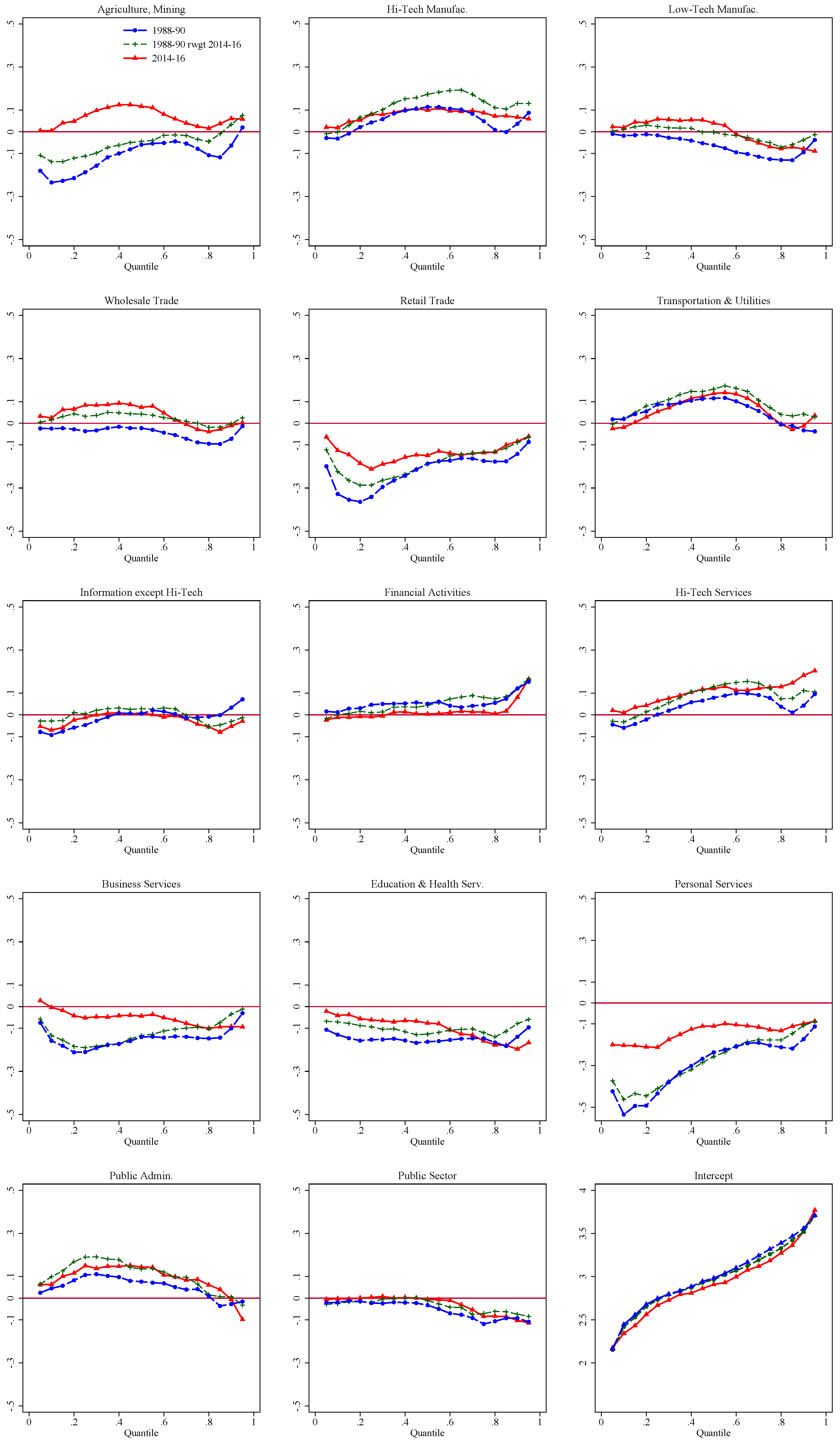
Figure 6.
Decomposition of Total Change into Composition and Wage Structure Effects.

Figure 7.
Decomposition of Composition Effects.

Figure 8.
Decomposition of Wage Structure Effects.

Table 1.
Unconditional Quantile Regression Coefficients on Log Wages.
| Years: | 1988/90 | 2014/16 | ||||
|---|---|---|---|---|---|---|
| Quantiles: | 10 | 50 | 90 | 10 | 50 | 90 |
| Explanatory Variables | ||||||
| Union covered | 0.146 | 0.343 | −0.025 | 0.058 | 0.240 | −0.008 |
| (0.003) | (0.005) | (0.004) | (0.003) | (0.006) | (0.007) | |
| Non-white | −0.063 | −0.137 | −0.072 | −0.053 | −0.106 | −0.041 |
| (0.006) | (0.005) | (0.005) | (0.004) | (0.004) | (0.006) | |
| Non-Married | −0.111 | −0.109 | −0.031 | −0.046 | −0.107 | −0.064 |
| (0.004) | (0.003) | (0.004) | (0.003) | (0.004) | (0.005) | |
| Education (High School omitted) | ||||||
| Primary | −0.301 | −0.312 | −0.109 | −0.212 | −0.415 | −0.110 |
| (0.011) | (0.006) | (0.005) | (0.01) | (0.009) | (0.006) | |
| Some HS | −0.305 | −0.112 | 0.005 | −0.275 | −0.215 | 0.002 |
| (0.007) | (0.005) | (0.003) | (0.008) | (0.007) | (0.004) | |
| Some College | 0.055 | 0.135 | 0.112 | 0.036 | 0.098 | 0.023 |
| (0.005) | (0.004) | (0.005) | (0.004) | (0.005) | (0.004) | |
| College | 0.143 | 0.343 | 0.410 | 0.125 | 0.409 | 0.493 |
| (0.005) | (0.005) | (0.008) | (0.004) | (0.006) | (0.009) | |
| Post-grad | 0.094 | 0.418 | 0.772 | 0.099 | 0.502 | 0.962 |
| (0.006) | (0.006) | (0.013) | (0.004) | (0.008) | (0.017) | |
| Potential Experience (20 ≤ Experience < 25 omitted) | ||||||
| Experience < 5 | −0.486 | −0.448 | −0.312 | −0.335 | −0.425 | −0.301 |
| (0.009) | (0.006) | (0.008) | (0.007) | (0.007) | (0.011) | |
| 5 ≤ Experience < 10 | −0.056 | −0.270 | −0.278 | −0.067 | −0.285 | −0.306 |
| (0.006) | (0.006) | (0.008) | (0.005) | (0.007) | (0.011) | |
| 10 ≤ Experience < 15 | −0.005 | −0.122 | −0.172 | −0.022 | −0.157 | −0.182 |
| (0.005) | (0.006) | (0.008) | (0.004) | (0.006) | (0.011) | |
| 15 ≤ Experience < 20 | 0.002 | −0.051 | −0.091 | −0.009 | −0.051 | −0.034 |
| (0.005) | (0.005) | (0.008) | (0.004) | (0.006) | (0.012) | |
| 25 ≤ Experience < 30 | 0.010 | 0.033 | 0.060 | −0.001 | 0.020 | 0.036 |
| (0.006) | (0.006) | (0.01) | (0.004) | (0.006) | (0.012) | |
| 30 ≤ Experience < 35 | 0.017 | 0.048 | 0.071 | 0.008 | 0.037 | 0.042 |
| (0.006) | (0.006) | (0.011) | (0.004) | (0.007) | (0.012) | |
| 35 ≤ Experience < 40 | 0.022 | 0.028 | 0.061 | 0.013 | 0.054 | 0.062 |
| (0.007) | (0.008) | (0.012) | (0.004) | (0.007) | (0.013) | |
| Experience ≥ 40 | 0.068 | 0.020 | −0.010 | 0.030 | 0.058 | −0.013 |
| (0.008) | (0.008) | (0.009) | (0.005) | (0.007) | (0.012) | |
| R−square | 0.253 | 0.359 | 0.206 | 0.182 | 0.353 | 0.202 |
| No. of observations | 268,494 | 236,296 | ||||
Note: Linear limited dependent variable model. Bootstrapped standard errors (500 repetitions) are in parentheses. Statistical signifiance levels: p ≤ 0.01, p ≤ 0.05, p ≤ 0.1. Also included in the regression are a public sector dummy, 16 occupation dummies, and 14 industry dummies. The base group is made up of individuals who are non-unionized (not covered), not in the public sector, white, married, have a high school degree, work as construction workers in the construction industry.
Table 2.
RIF Regression of Inequality Measures.
| Years: | 1988/90 | 2014/16 | 1988/90 | 2014/16 |
|---|---|---|---|---|
| Inequality Measures | Variance of Log Wages | Gini | ||
| Estimated Values: | 0.341 | 0.418 | 0.330 | 0.396 |
| Explanatory Variables | ||||
| Constant | 0.203 | 0.205 | 0.261 | 0.290 |
| (0.004) | (0.006) | (0.002) | (0.002) | |
| Union covered | −0.075 | −0.040 | −0.067 | −0.039 |
| (0.002) | (0.004) | (0.001) | (0.001) | |
| Non-white | −0.002 | 0.005 | 0.006 | 0.005 |
| (0.003) | (0.004) | (0.001) | (0.001) | |
| Non-Married | 0.039 | 0.001 | 0.022 | 0.008 |
| (0.002) | (0.004) | (0.001) | (0.001) | |
| Education (High School omitted) | ||||
| Primary | 0.074 | 0.073 | 0.051 | 0.057 |
| (0.004) | (0.006) | (0.002) | (0.002) | |
| Some HS | 0.104 | 0.129 | 0.048 | 0.063 |
| (0.003) | (0.005) | (0.001) | (0.001) | |
| Some College | 0.028 | −0.001 | 0.006 | −0.006 |
| (0.003) | (0.003) | (0.002) | (0.003) | |
| College | 0.121 | 0.166 | 0.053 | 0.061 |
| (0.005) | (0.005) | (0.002) | (0.001) | |
| Post-grad | 0.301 | 0.401 | 0.157 | 0.177 |
| (0.007) | (0.01) | (0.003) | (0.002) | |
| Potential Experience (20 ≤ Experience < 25 omitted) | ||||
| Experience < 5 | 0.047 | 0.027 | 0.031 | 0.021 |
| (0.004) | (0.007) | (0.002) | (0.002) | |
| 5 ≤ Experience < 10 | −0.098 | −0.093 | −0.036 | −0.030 |
| (0.005) | (0.007) | (0.002) | (0.002) | |
| 10 ≤ Experience < 15 | −0.078 | −0.070 | −0.035 | −0.028 |
| (0.004) | (0.007) | (0.002) | (0.002) | |
| 15 ≤ Experience < 20 | −0.050 | −0.006 | −0.026 | 0.003 |
| (0.005) | (0.008) | (0.002) | (0.002) | |
| 25 ≤ Experience < 30 | 0.023 | 0.024 | 0.012 | 0.014 |
| (0.006) | (0.008) | (0.002) | (0.002) | |
| 30 ≤ Experience < 35 | 0.022 | 0.017 | 0.008 | 0.007 |
| (0.006) | (0.008) | (0.002) | (0.002) | |
| 35 ≤ Experience < 40 | 0.015 | 0.022 | 0.008 | 0.008 |
| (0.007) | (0.008) | (0.003) | (0.002) | |
| Experience ≥ 40 | −0.031 | −0.012 | −0.015 | −0.005 |
| (0.005) | (0.008) | (0.003) | (0.002) | |
| Occupations (Construction & Repair Occ. omitted) | ||||
| Upper Management | 0.235 | 0.415 | 0.132 | 0.203 |
| (0.007) | (0.011) | (0.003) | (0.002) | |
| Lower Management | 0.090 | 0.200 | 0.027 | 0.080 |
| (0.008) | (0.009) | (0.003) | (0.002) | |
| Engineers & Computer Occ. | 0.107 | 0.202 | 0.013 | 0.054 |
| (0.006) | (0.009) | (0.003) | (0.002) | |
| Other Scientists | 0.081 | 0.134 | 0.025 | 0.068 |
| (0.011) | (0.027) | (0.005) | (0.006) | |
| Social Support Occ. | −0.001 | 0.065 | −0.012 | 0.012 |
| (0.007) | (0.009) | (0.003) | (0.003) | |
| Lawyers & Doctors | 0.524 | 0.637 | 0.337 | 0.363 |
| (0.027) | (0.032) | (0.010) | (0.008) | |
| Health Treatment Occ. | −0.020 | 0.115 | −0.035 | 0.011 |
| (0.0101) | (0.012) | (0.005) | (0.005) | |
| Clerical Occ. | 0.013 | 0.069 | 0.017 | 0.044 |
| (0.004) | (0.005) | (0.002) | (0.002) | |
| Explanatory Variables | ||||
| Occupations (cnt.) | ||||
| Sales Occ. | 0.088 | 0.177 | 0.043 | 0.084 |
| (0.005) | (0.008) | (0.002) | (0.002) | |
| Insur. & Real Estate Sales | 0.208 | 0.197 | 0.152 | 0.105 |
| (0.031) | (0.038) | (0.011) | (0.010) | |
| Financial Sales | 0.525 | 0.409 | 0.429 | 0.219 |
| (0.06) | (0.076) | (0.018) | (0.014) | |
| Service Occ. | 0.188 | 0.208 | 0.101 | 0.107 |
| (0.004) | (0.005) | (0.002) | (0.002) | |
| Primary Occ. | 0.226 | 0.222 | 0.114 | 0.127 |
| (0.008) | (0.015) | (0.004) | (0.004) | |
| Production Occ. | 0.004 | 0.020 | 0.011 | 0.028 |
| (0.003) | (0.005) | (0.001) | (0.002) | |
| Transportation Occ. | 0.119 | 0.145 | 0.079 | 0.094 |
| (0.004) | (0.006) | (0.002) | (0.002) | |
| Truckers | 0.015 | 0.042 | 0.030 | 0.040 |
| (0.004) | (0.006) | (0.002) | (0.002) | |
| Industries (Construction omitted) | ||||
| Agriculture, Mining | 0.079 | 0.013 | 0.036 | −0.001 |
| (0.008) | (0.012) | (0.003) | (0.003) | |
| Hi-Tech Manufac | 0.018 | 0.014 | −0.001 | 0.002 |
| (0.005) | (0.009) | (0.002) | (0.002) | |
| Low-Tech Manufac | −0.037 | −0.053 | −0.011 | −0.019 |
| (0.004) | (0.007) | (0.002) | (0.002) | |
| Wholesale Trade | −0.012 | −0.027 | 0.001 | −0.006 |
| (0.006) | (0.012) | (0.002) | (0.003) | |
| Retail Trade | 0.060 | 0.016* | 0.038 | 0.023 |
| (0.005) | (0.007) | (0.002) | (0.002) | |
| Transportation & Utilities | 0.013 | −0.029 | −0.005 | −0.019 |
| (0.005) | (0.007) | (0.002) | (0.002) | |
| Information except Hi-Tech | −0.001 | 0.055 | −0.010 | 0.041 |
| (0.008) | (0.019) | (0.003) | (0.005) | |
| Financial Activities | 0.065 | 0.064 | 0.052 | 0.053 |
| (0.009) | (0.013) | (0.004) | (0.003) | |
| Hi-Tech Services | 0.048 | 0.071 | 0.018 | 0.035 |
| (0.008) | (0.01) | (0.004) | (0.003) | |
| Business Services | 0.018 | −0.042 | 0.019 | −0.014 |
| (0.005) | (0.008) | (0.002) | (0.002) | |
| Education & Health Services | −0.008 | −0.064 | −0.001 | −0.018 |
| (0.006) | (0.008) | (0.003) | (0.002) | |
| Personal Services | 0.136 | 0.054 | 0.051 | 0.023 |
| (0.006) | (0.006) | (0.002) | (0.002) | |
| Public Admin | −0.038 | −0.071 | −0.036 | −0.029 |
| (0.007) | (0.011) | (0.003) | (0.003) | |
| Public Sector | −0.058 | −0.055 | −0.030 | −0.048 |
| (0.005) | (0.007) | (0.002) | (0.002) | |
| R-squared | 0.115 | 0.087 | 0.048 | 0.025 |
| No. of observations | 268,492 | 236,287 | 268,492 | 236,287 |
Note: Bootstrapped standard errors (500 repetitions) are in parentheses. Statistical signifiance levels: *** p ≤ 0.01, ** p ≤ 0.05, * p ≤ 0.1. The base group is made up of individuals who are non-unionized (not covered), not public sector, white, married, have a high school degree, work as construction workers in the construction industry. Trimmed sample drops 15 observations with hourly wages > $1,636 ($2010).
Table 3.
Decomposition Results without Reweighting.
| Inequality Measures | 90–10 | 50–10 | 90–50 | Variance (× 100) | Gini (× 100) |
|---|---|---|---|---|---|
| Total Change | 0.125 | −0.075 | 0.201 | 7.775 | 6.599 |
| Composition | 0.089 | 0.037 | 0.052 | 4.163 | 1.966 |
| Wage Structure | 0.037 | −0.112 | 0.149 | 3.612 | 4.633 |
| Composition Effects: | |||||
| Union | 0.016 | −0.019 | 0.035 | 0.713 | 0.639 |
| Other | 0.019 | 0.008 | 0.011 | 0.984 | 0.473 |
| Education | 0.009 | 0.013 | −0.005 | 0.665 | 0.207 |
| Occupation | 0.019 | 0.022 | −0.002 | 0.672 | 0.112 |
| Industry | 0.026 | 0.013 | 0.013 | 1.128 | 0.536 |
| Wage Structure Effects: | |||||
| Union | 0.014 | −0.002 | 0.015 | 0.442 | 0.360 |
| Other | −0.048 | −0.034 | −0.014 | −0.983 | −0.161 |
| Education | 0.015 | 0.008 | 0.007 | 1.444 | 0.188 |
| Occupation | 0.057 | −0.066 | 0.123 | 5.664 | 2.423 |
| Industry | −0.079 | −0.048 | −0.031 | −3.212 | −1.044 |
| Constant | 0.079 | 0.030 | 0.049 | 0.257 | 0.287 |
| Total Effects: | |||||
| Union | 0.030 | −0.021 | 0.051 | 1.156 | 0.998 |
| Other | −0.029 | −0.026 | −0.003 | 0.001 | 0.312 |
| Education | 0.024 | 0.022 | 0.002 | 2.110 | 0.395 |
| Occupation | 0.076 | −0.045 | 0.121 | 6.336 | 2.534 |
| Industry | −0.054 | −0.036 | −0.018 | −2.084 | −0.508 |
Note: Other includes non-white, non-married, and five categories of experience. Statistical signifiance levels: p ≤ 0.01, p ≤ 0.05, p ≤ 0.1. Bootstrapped standard errors over the entire procedure (500 replications) were used to compute the p-value. Trimmed sample for the variance and Gini drops 15 observations with hourly wages > $1,636 ($2010).
Table 4.
Decomposition Results with Reweighting.
| Inequality Measures | 90–10 | 50–10 | 90–50 | Variance (× 100) | Gini (× 100) |
|---|---|---|---|---|---|
| Total Change | 0.125 | −0.075 | 0.201 | 7.775 | 6.599 |
| Composition | 0.090 | 0.038 | 0.052 | 4.193 | 1.966 |
| Wage Structure | 0.030 | −0.105 | 0.135 | 3.149 | 4.402 |
| Composition Effects: | |||||
| Union | 0.016 | −0.019 | 0.035 | 0.712 | 0.638 |
| Other | 0.019 | 0.009 | 0.011 | 1.007 | 0.481 |
| Education | 0.007 | 0.013 | −0.005 | 0.600 | 0.173 |
| Occupation | 0.020 | 0.022 | −0.002 | 0.719 | 0.129 |
| Industry | 0.026 | 0.013 | 0.014 | 1.155 | 0.546 |
| Specification Error | 0.002 | −0.010 | 0.012 | −0.308 | 0.175 |
| Wage Structure Effects: | |||||
| Union | 0.012 | −0.005 | 0.017 | 0.338 | 0.220 |
| Other | −0.049 | −0.026 | −0.023 | −0.871 | −0.068 |
| Education | 0.054 | 0.010 | 0.045 | 2.303 | 1.183 |
| Occupation | 0.018 | −0.075 | 0.093 | 2.872 | 1.416 |
| Industry | −0.094 | −0.030 | −0.064 | −3.852 | −1.306 |
| Constant | 0.089 | 0.022 | 0.067 | 2.359 | 2.957 |
| Reweighting Error | 0.003 | 0.002 | 0.001 | 0.125 | 0.057 |
| Total Effects: | |||||
| Union | 0.029 | −0.024 | 0.052 | 1.050 | 0.857 |
| Other | −0.029 | −0.018 | −0.012 | 0.135 | 0.413 |
| Education | 0.062 | 0.022 | 0.039 | 2.903 | 1.356 |
| Occupation | 0.038 | −0.053 | 0.091 | 3.591 | 1.545 |
| Industry | −0.068 | −0.017 | −0.051 | −2.697 | −0.760 |
Note: Other includes non-white, non-married, and five categories of experience. Statistical signifiance levels: p ≤ 0.01, p ≤ 0.05, p ≤ 0.1. Bootstrapped standard errors over the entire procedure (500 replications) were used to compute the p-value. Trimmed sample for the variance and Gini drops 15 observations with hourly wages > $1,636 ($2010).
© 2018 by the authors. Licensee MDPI, Basel, Switzerland. This article is an open access article distributed under the terms and conditions of the Creative Commons Attribution (CC BY) license (http://creativecommons.org/licenses/by/4.0/).
Share and Cite
MDPI and ACS Style
Firpo, S.P.; Fortin, N.M.; Lemieux, T. Decomposing Wage Distributions Using Recentered Influence Function Regressions. Econometrics 2018, 6, 28. https://0-doi-org.brum.beds.ac.uk/10.3390/econometrics6020028
AMA Style
Firpo SP, Fortin NM, Lemieux T. Decomposing Wage Distributions Using Recentered Influence Function Regressions. Econometrics. 2018; 6(2):28. https://0-doi-org.brum.beds.ac.uk/10.3390/econometrics6020028
Chicago/Turabian StyleFirpo, Sergio P., Nicole M. Fortin, and Thomas Lemieux. 2018. "Decomposing Wage Distributions Using Recentered Influence Function Regressions" Econometrics 6, no. 2: 28. https://0-doi-org.brum.beds.ac.uk/10.3390/econometrics6020028
Note that from the first issue of 2016, this journal uses article numbers instead of page numbers. See further details here.