The Relation between Monetary Policy and the Stock Market in Europe

Abstract

We use a cointegrated structural vector autoregressive model to investigate the relation between monetary policy in the euro area and the stock market. Since there may be an instantaneous causal relation, we consider long-run identifying restrictions for the structural shocks and also used (conditional) heteroscedasticity in the residuals for identification purposes. Heteroscedasticity is modelled by a Markov-switching mechanism. We find a plausible identification scheme for stock market and monetary policy shocks which is consistent with the second-order moment structure of the variables. The model indicates that contractionary monetary policy shocks lead to a long-lasting downturn of real stock prices.

1. Introduction

The interaction of monetary policy and the stock market has been studied extensively with structural vector autoregressive (VAR) models. A central problem is the identification of the structural shocks. Nowadays, a range of different tools is available for identifying structural VARs (see Kilian and Lütkepohl 2017). Therefore, different types of identifying restrictions for monetary policy and stock market shocks have been used. For example, Bjørnland and Leitemo (2009) considered a structural VAR model for the US, where long-run and short-run restrictions were combined to identify structural shocks. Such models were also used in the context of identification by heteroscedasticity (e.g., Lütkepohl and Netšunajev 2017a, 2017b; Bertsche and Braun 2018). All these studies investigated the relation between monetary policy and the stock market in the US, but they ignored that the variables may be cointegrated. In the present study, we consider the relation between monetary policy and the stock market in Europe and explicitly account for possible cointegration of the variables involved.

European monetary policy is, of course, a central topic of empirical macroeconomics (e.g., Peersman and Smets 2001). There are also studies investigating explicitly the impact of monetary policy in Europe on the stock market. Cassola and Morana (2004) found that price-stabilizing monetary policy contributes to the stability of the stock market in the euro area. Bredin et al. (2009) performed an event study and found a negative relation between UK monetary policy and stock returns, but not between German monetary policy and stock returns. Kholodilin et al. (2009) used the approach of Rigobon and Sack (2004) and found heterogeneous relations between monetary policy and stock prices for different sectors, but the effect of an increase in the policy rate of the European Central Bank (ECB) on an aggregate stock index was reported to be negative. Haitsma et al. (2016) identified the ECB monetary policy shocks using an event-study approach and via heteroscedasticity following Rigobon and Sack (2004). Both identification methods yielded a negative relationship between unexpected changes in policy rates and stock returns. Alessi and Kerssenfischer (2016) estimated a structural factor model using euro area data and argued that the responses of stock returns to monetary policy are larger and quicker than in a conventional small-scale structural VAR. In a more recent study, Fausch and Sigonius (2018) used different techniques to investigate the relation between ECB monetary policy and German stock returns, including an event study, a VAR analysis—where monetary policy surprises are captured by a proxy variable—and a threshold VAR model. They found a negative relation between the ECB monetary policy and stock returns in the pre-crisis period.

In this study, we use a structural vector error correction model (VECM) identified through heteroscedasticity to investigate the relation between monetary policy and the stock market. The cointegration framework developed by Johansen and Juselius (see Johansen and Juselius 1990; Johansen 1991, 1995; Juselius 2006) opens up a convenient way to impose restrictions on the long-run effects of structural shocks in structural VAR analysis, as shown by King et al. (1991). They used the Granger–Johansen representation of a VAR model (Johansen 1995) to determine the long-run effects of their shocks, and the framework is easy to combine with identifying information obtained from the second-moment structure of the model (see Lütkepohl and Velinov 2016 or Kilian and Lütkepohl 2017, chp. 14). We use this framework in our empirical investigation.

We model the conditional heteroscedasticity in the data by a Markov-switching (MS) mechanism and find a cointegrated structural VAR model for which conventional identifying restrictions are in line with the second-moment structure of the data. The impulse responses are plausible and, in particular, production and price level go down after a contractionary monetary policy shock. Although the long-run impact of a monetary policy shock on stock prices is restricted to zero, such a shock is found to have a rather long-lasting negative impact on the stock market.

The structure of this study is as follows. In the next section, the basic structural VECM is presented and the model for the second moments is discussed in Section 3. The empirical analysis is considered in Section 4 and conclusions are presented in Section 5. The Appendix A provides details on the data sources.

2. Structural Vector Error Correction Models

The time series variables of interest are collected in the $(K\times 1)$ vector $y_t$. The components of $y_t$ may be integrated and cointegrated variables. We assume that all variables are stationary ($I(0)$) or integrated of order one ($I(1)$). Assuming a cointegration rank r, $0\le r\le K$, our point of departure is the VECM form of a VAR model,

$$\Delta y_t=\nu +\alpha {\beta }^{\prime }{y}_{t-1}+{\Gamma }_1\Delta y_{t-1}+\cdots +{\Gamma }_{p-1}\Delta y_{t-p+1}+u_t,$$

(1)

where $\Delta$ is the differencing operator such that $\Delta y_t=y_t-y_{t-1}$, $\nu$ is a $(K\times 1)$ constant intercept term, $\alpha$ is a $(K\times r)$ loading matrix of rank r, $\beta$ is a $(K\times r)$ cointegration matrix of rank r, and ${\Gamma }_1,\dots ,{\Gamma }_{p-1}$ are $(K\times K)$ coefficient matrices (see also Johansen 1995).

The reduced-form residuals $u_t$ are white noise, that is, $u_t$ is serially uncorrelated with mean zero but may have time-varying second moments. In other words, $u_t$ may be heteroscedastic or conditionally heteroscedastic. The structural shocks, denoted by ${\epsilon }_t$, are obtained from the reduced-form residuals by a linear transformation ${\epsilon }_t=B^{-1}{u}_t$ or $B{\epsilon }_t=u_t$. The $(K\times K)$ transformation matrix B is assumed to be such that the structural shocks are instantaneously uncorrelated. Hence, $\mathbb{E}({\epsilon }_t{\epsilon }_t^{\prime })={\Sigma }_{{\epsilon }_t}$ is a diagonal matrix.

Substituting $B{\epsilon }_t$ for $u_t$ in (1), the matrix B is easily recognized as the matrix of impact effects of the structural shocks. Thus, imposing restrictions directly on the impact effects means putting restrictions on the elements of B. Typically, zero restrictions are imposed on B, which implies that certain variables do not respond instantaneously to a shock.

The long-run effects of the shocks are easily obtained through the Granger–Johansen representation (see Johansen (1995, Theorem 4.2)) of $y_t$ corresponding to (1),

$$y_t=\Xi \sum _{i=1}^t{u}_i+{\Xi }^{\ast }(L)u_t+{\delta }_t+y_0^{\ast },$$

(2)

where

$$\Xi ={\beta }_{\perp }{\left[{\alpha }_{\perp }^{\prime }\left(I_K-\sum _{i=1}^{p-1}{\Gamma }_i\right){\beta }_{\perp }\right]}^{-1}{\alpha }_{\perp }^{\prime },$$

(3)

${\Xi }^{\ast }(L)u_t$ is a stationary process, ${\delta }_t$ contains deterministic terms, and $y_0^{\ast }$ represents initial conditions. In (3), ${\beta }_{\perp }$ and ${\alpha }_{\perp }$ are $(K\times (K-r))$ dimensional orthogonal complements of the $(K\times r)$ dimensional matrices $\beta$ and $\alpha$, respectively. If the cointegration rank r is zero, the orthogonal complement matrices are replaced by $(K\times K)$ identity matrices so that the long-run effects matrix becomes

$$\Xi ={\left(I_K-\sum _{i=1}^{p-1}{\Gamma }_i\right)}^{-1}.$$

(4)

The corresponding long-run effects of the structural shocks are given by $\Xi B$. Since $\alpha$ and $\beta$ have rank r, their orthogonal complements have rank $K-r$, implying that $\Xi$ also has rank $K-r$, and the same holds for $\Xi B$ because B is an invertible matrix of full rank K. For a given reduced-form matrix $\Xi$, restrictions on $\Xi B$ imply restrictions for B and, hence, can help identify the structural shocks. The reduced rank of the long-run effects matrix implies that there can be at most r shocks without any long-run effects, corresponding to r columns of zeros of $\Xi B$. In other words, only r shocks can be purely transitory. Another side effect of the reduced rank of $\Xi B$ is, however, that simply counting zero restrictions is not enough to assess identification of the structural matrix B, as we will see in our empirical application in Section 4.

This setup for identifying structural shocks in VAR models was proposed by King et al. (1991). Introductory treatments are given by Lütkepohl (2005, chp. 9) and Kilian and Lütkepohl (2017, chp. 10). An advantage of the structural VECM setup is that only the cointegration rank is needed, which implies the rank of the long-run effects matrix $\Xi B$. Knowing that rank, the structural shocks can be properly specified through long-run restrictions. Typically the actual cointegration relations are not needed. Thus, pretesting for specific cointegration relations and even knowing the precise order of integration of specific variables is not necessary, as long as the cointegration rank is known.

There are a number of situations of special interest. For $r=0$, the matrix of long-run effects $\Xi B$ is of full rank K and, hence, cannot have zero columns. Thus, for $r=0$, all K structural shocks have some long-run effects. If the cointegrating rank is zero, the VECM (1) reduces to a VAR model in first differences,

$$\Delta y_t=\nu +{\Gamma }_1\Delta y_{t-1}+\cdots +{\Gamma }_{p-1}\Delta y_{t-p+1}+u_t,$$

for which the accumulated long-run effects on the $\Delta y_t$ are known to be

$${\left(I_K-\sum _{i=1}^{p-1}{\Gamma }_i\right)}^{-1}B.$$

The accumulated effects on the first differences are just the long-run effects on the levels $y_t$, of course. This case was considered by Blanchard and Quah (1989), and the estimation of the structural parameters, i.e., the B matrix, is particularly easy for this case (e.g., Lütkepohl (2005, chp. 9)).

If some of the components of $y_t$ are $I(0)$, the long-run effects matrix $\Xi$ and, hence, also $\Xi B$, has corresponding rows of zero elements because a stationary variable is not affected permanently by a shock. Formally, that can be seen by dividing up the vector

$$y_t=\left[\begin{array}{c}{y}_t^n\\ y_t^s\end{array}\right],$$

where all components of the $(K_n\times 1)$ vector $y_t^n$ are $I(1)$ and all components of the $(K_s\times 1)$ vector $y_t^s$ are $I(0)$. In this case there exists a cointegration matrix of the form

$$\beta =\left[\begin{array}{cc}{\beta }_{(11)}& 0_{K_n\times K_s}\\ 0_{K_s\times (r-K_s)}& I_{K_s}\end{array}\right],$$

where ${\beta }_{(11)}$ is a $(K_n\times (r-K_s))$ matrix and $0_{M\times N}$ denotes a $(M\times N)$ zero matrix. Thus, there exists an orthogonal complement of $\beta$ such that

$${\beta }_{\perp }=\left[\begin{array}{c}{\beta }_{\perp }^{(1)}\\ 0_{K_s\times (K-r)}\end{array}\right].$$

Hence, the last $K_s$ rows of $\Xi$ are rows of zeros.

There are alternative proposals for imposing long-run restrictions for identifying structural shocks in VARs. Examples are proposals by Gonzalo and Ng (2001); Fisher et al. (2000), and Pagan and Pesaran (2008). Fisher and Huh (2014) review the literature and discuss the relations between alternative approaches.

3. Structural VAR Models with Changes in Volatility

If the reduced-form residuals $u_t$ are heteroscedastic or conditionally heteroscedastic, this property can be used for identification purposes. We use the approach of Lanne et al. (2010) and Herwartz and Lütkepohl (2014), who proposed a Markov-switching (MS) mechanism for modelling volatility changes in this context. They assumed that the distribution of the error term $u_t$ depends on a discrete Markov process $s_t$, such that

$$u_t|s_t\sim (0,{\Sigma }_u(s_t)).$$

(5)

The Markov process $s_t$ has states $1,\dots ,M$ and transition probabilities

$$p_{ij}=\mathrm{Pr}(s_t=j|s_{t-1}=i),i,j=1,\dots ,M.$$

Note that only the residual covariance matrices depend on the state $s_t$, whereas the VAR slope parameters are not state dependent. The model captures conditional heteroscedasticity of a quite general form.

The second-moment structure can be used for structural identification if the covariance matrices can be decomposed such that

$${\Sigma }_u(1)=B{B}^{\prime },{\Sigma }_u(m)=B{\Lambda }_m{B}^{\prime },m=2,\dots ,M,$$

(6)

where the ${\Lambda }_m$ are $(K\times K)$ diagonal matrices. In that case, the matrix B can be used to obtain the structural shocks from the reduced-form residuals, and B is identified if the following condition holds, where ${\lambda }_{jk}$ denotes the kth diagonal element of ${\Lambda }_j$:

$$\forall k,l\in \{1,\dots ,K\}\exists j\in \{2,\dots ,M\}\mathrm{such}\mathrm{that}{\lambda }_{jk}\ne {\lambda }_{jl}.$$

(7)

If $M=2$, the condition means that the diagonal elements of ${\Lambda }_2$ must all be distinct. Generally, the condition requires that there is sufficient heterogeneity in the volatility changes across the shocks. If this condition is satisfied, B is unique up to column sign changes and column permutations. In other words, using this B matrix for computing the structural shocks from the reduced-form residuals, only the sign and positioning of the shocks remain undetermined. Note, however, that this identification approach relies on the assumption that the impact effects of the shocks remain time-invariant and only the variances change over time.

Assuming a normal conditional distribution for $u_t|s_t$, the model can be estimated by Gaussian maximum likelihood (ML) using the algorithm described by Herwartz and Lütkepohl (2014). It may be useful to estimate the cointegration matrix $\beta$ in a first step and keep it fixed in the subsequent optimisation of the log-likelihood with respect to the remaining parameters, including the transition probabilities. Computing the Gaussian ML estimates can be a challenge for larger models with many variables, autoregressive lags, or volatility states.

The fact that the model assigns the volatility regimes endogenously is appealing. Hence, the researcher can estimate the volatility states rather than having to know or assume them. We use the model in our empirical application, which is discussed in the next section.

4. Monetary Policy and the Stock Market in Europe

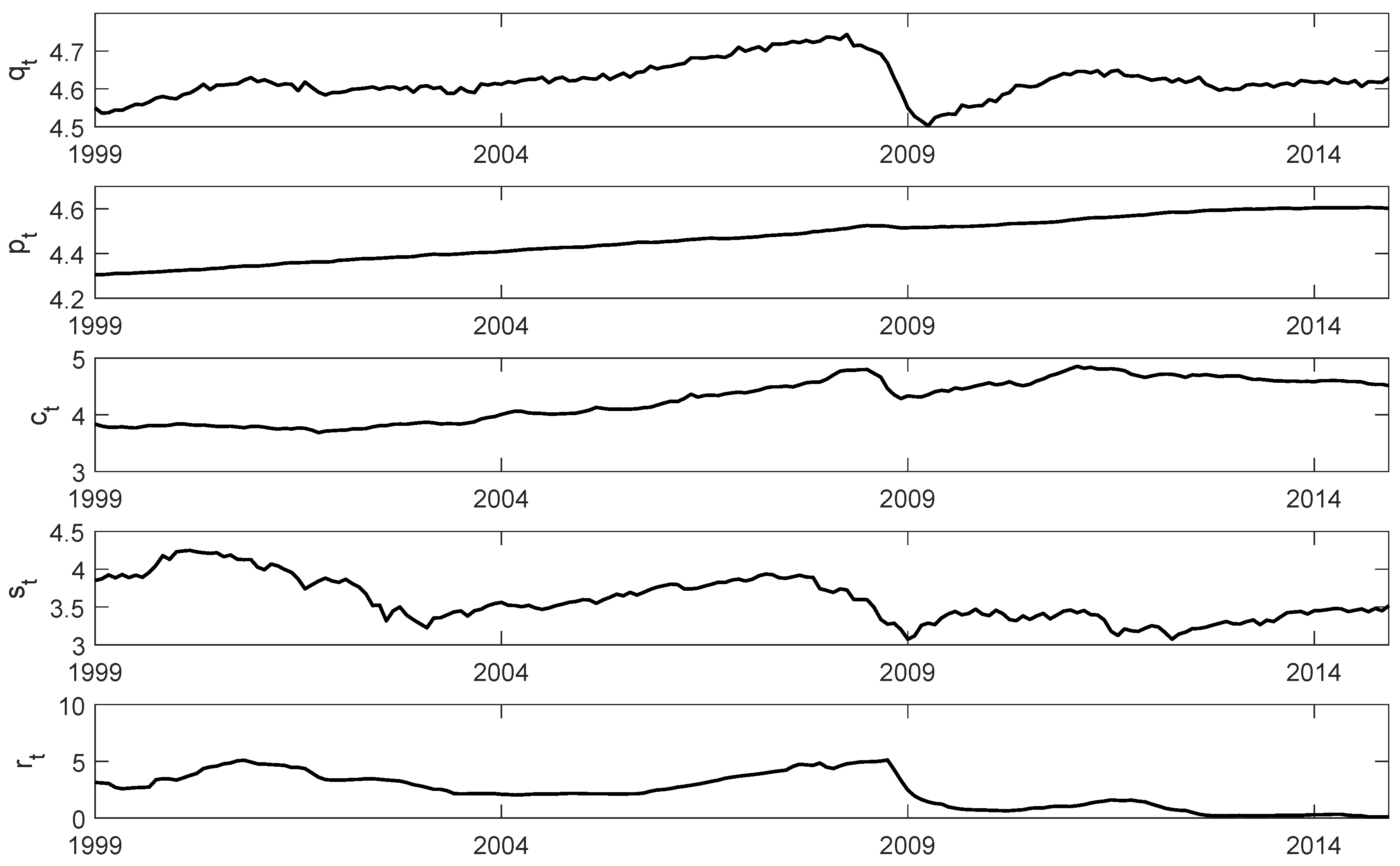
A five-dimensional VAR model for the euro area with variables $y_t={(q_t,p_t,c_t,s_t,r_t)}^{\prime }$ is considered, where $q_t$ is the log of an industrial production index, $p_t$ denotes the log of the harmonized index of consumer prices (HICP), $c_t$ is a log non-energy commodity price index, $s_t$ is the log of the real Euro Stoxx 50 stock price index, and $r_t$ denotes the 3 month Euribor. The set of variables corresponds to the system used by Bjørnland and Leitemo (2009) for analysing the relation between monetary policy and the stock market in the US. We use monthly data for the period 1999M1–2014M12 and, hence, avoid the period of quantitative easing in the eurozone. Further details on the variables and data sources are given in the appendix, and the time series are plotted in Figure 1.

Given the substantial impact of the financial crisis in 2008 following the collapse of Lehman Brothers, one may wonder whether a time-invariant VAR or VECM is appropriate for the full sample period. We have therefore fitted VAR(2) models for $y_t={(q_t,p_t,c_t,s_t,r_t)}^{\prime }$, where all or some of the coefficients are allowed to vary over time. The time-variation is governed by a two-state MS mechanism. Some models are compared in

Table 1. Comparison of Markov-switching vector autoregressive models for $y_t={(q_t,p_t,c_t,s_t,r_t)}^{\prime }$.

Model	Log L	AIC	SC	HQ
VAR(2)	2514.761	$-4889.522$	$-4662.230$	$-4797.449$
VAR(2)-MSIAH(2)	2668.241	$-5052.483$	$-4591.405$	$-4858.779$
VAR(2)-MSIH(2)	2617.071	$-5050.142$	$-4750.452$	$-4928.766$
VAR(2)-MSH(2)	2611.456	$-5048.912$	$-4766.421$	$-4934.479$

Note: L—Gaussian likelihood, AIC = $-2\log L+2\times$ number of free parameters, SC = $-2\log L+\log T\times$ number of free parameters, HQ = $-2\log L+2\times \mathrm{number}\mathrm{of}\mathrm{free}\mathrm{parameters}\times \log (\log T)$. MSIAH—model with time-varying intercept, VAR slope coefficients and error covariance matrix; MSIH—model with time-varying intercept and error covariance matrix; MSH—model with time-varying error covariance matrix but time-invariant intercept and VAR slope coefficients.

, using standard model selection criteria. The abbreviations used in Table 1 follow those proposed by Krolzig (1997), that is, MSIAH stands for a VAR model with time-varying intercept, VAR slope coefficients, and error covariance matrix; MSIH abbreviates a model where only the intercept vector and the error covariance matrix are allowed to vary; and MSH signifies a model with time-invariant intercept and VAR slope coefficients but varying error covariance matrix. In all cases, two Markov states are used, which is indicated in parentheses behind the model abbreviation. A lag order of $p=2$ is suggested by the Akaike information criterion (AIC), the Schwarz Criterion (SC), and the Hannan–Quinn criterion (HQ) (see Lütkepohl (2005, sct. 4.3)) for a time-invariant VAR process for the full sample period. Thus, in Table 1, for example, VAR(2)-MSH(2) signifies a VAR model of order 2 with 2 possible error covariance regimes and time-invariant intercept and VAR slope coefficients. It turns out that such a model is favoured by the SC and HQ model selection criteria, while AIC favours a fully flexible model. Provided the quantitative easing period is excluded from the sample, it is reasonable to believe that the monetary policy regime has not changed. With that in mind, and taking into account the preferences of the SC and HQ criteria, we use the model with time-invariant intercepts and slope coefficients and allow for a time-varying error covariance matrix only in the following. We decompose the covariance matrices such that time-invariant impact effects and time-invariant impulse responses are identified.

Based on conventional ADF tests, all five variables are classified as $I(1)$ variables. Thus, there may be cointegration among the variables, which is worth taking into account in our structural analysis. Since the VAR(2)-MSH(2) model, and thus a model with conditional heteroscedasticity, was favoured in the previous analysis, we base tests for the cointegration rank on Johansen’s (1995) cointegration rank tests robustified for conditional heteroscedasticity by generating the p-values with a wild bootstrap algorithm, as proposed by Cavaliere et al. (2010) and further investigated by Cavaliere et al. (2018). The results are presented in

Table 2. Testing for the cointegration rank of a VECM(1) with intercept for $y_t={(q_t,p_t,c_t,s_t,r_t)}^{\prime }$.

${\mathbb{H}}_{\mathbf{0}}$	LR Statistic	p-Value
$r=0$	70.570	0.036
$r\le 1$	59.559	0.001
$r\le 2$	20.539	0.081
$r\le 3$	6.227	0.482
$r\le 4$	0.248	0.978

Note: p-values are computed using Algorithm 1 of Cavaliere et al. (2010) with 1000 bootstrap replications.

and suggest a cointegration rank of $r=2$ if a 5% significance level is used. Thus, we consider a VECM(1) with one lag of the differenced variables (i.e., $p-1=1$) and cointegration rank $r=2$ for our structural analysis.

One advantage of imposing long-run restrictions on the long-run effects matrix $\Xi B$ obtained via the Granger–Johansen representation is that we do not have to take a stand on the exact cointegration relations, we just need to know the cointegration rank of the model. Imposing only the rank restriction is also in line with the original ideas behind structural VAR modelling, which imposes as few restrictions as possible. In this context, it is perhaps worth mentioning that Bjørnland and Leitemo (2009) considered a system $y_t={(q_t,\Delta p_t,\Delta c_t,\Delta s_t,r_t)}^{\prime }$ for US data which effectively assumes that there is no cointegration between the variables $p_t$, $c_t$ and $s_t$ so that these variables can be included in first differences. Although we do not want to reconsider the issue for US data here, it may be worth checking whether a setup with $\Delta p_t$, $\Delta c_t$, and $\Delta s_t$ instead of the levels variables can be used for European data as well, or whether the variables are potentially cointegrated. In

Table 3. Testing for the cointegration rank of a VECM(1) with intercept for $y_t={(p_t,c_t,s_t)}^{\prime }$.

${\mathbb{H}}_{\mathbf{0}}$	LR Statistic	p-Value
$r=0$	53.90	0.001
$r\le 1$	0.928	0.999
$r\le 2$	0.157	0.984

Note: p-values are computed using Algorithm 1 of Cavaliere et al. (2010) with 1000 bootstrap replications. The lag order of the VECM is suggested by HQ and SC.

, we present the results of cointegration rank tests and find clear evidence of cointegration between $p_t$, $c_t$, and $s_t$. Thus, the precise model specification used by Bjørnland and Leitemo (2009) would be difficult to defend for our European data, and we use the VECM(1) model with cointegration rank $r=2$ in the following. Another point worth emphasising is that this choice even accommodates the possibility that there are stationary variables in the model. For example, if there is a suspicion that the unit root tests have indicated unit roots just because of lack of power, this may be accommodated in our VECM setup as long as the cointegration tests indicate the cointegration rank adequately.

Based on the previous MS analysis we fit a volatility model of the type discussed in Section 3 with two states of the Markov process. The model is referred to as a VECM(1)-MSH(2) in the following. Given our small sample size, considering more volatility states is unreasonable.1 The AIC, HQ, and SC values of a VECM(1) model without allowing for heteroscedasticity and a VECM(1)-MSH(2) model are shown in

Table 4. Comparison of VECMs for $y_t={(q_t,p_t,c_t,s_t,r_t)}^{\prime }$.

Model	Log L	AIC	SC	HQ
VECM(1)	2505.139	$-4888.278$	$-4690.210$	$-4966.639$
VECM(1)-MSH(2)	2595.154	$-5034.308$	$-4781.040$	$-5134.507$

Note: L—Gaussian likelihood, AIC = $-2\log L+2\times$ number of free parameters, SC = $-2\log L+\log T\times$ number of free parameters, HQ = $-2\log L+2\times \mathrm{number}\mathrm{of}\mathrm{free}\mathrm{parameters}\times \log (\log T)$.

. They clearly signal that allowing for conditional heteroscedasticity improves the model fit. The values of all three model selection criteria are substantially smaller than the corresponding values for the model without heteroscedasticity. In other words, the second-moment structure may well provide useful identifying information for the structural shocks.

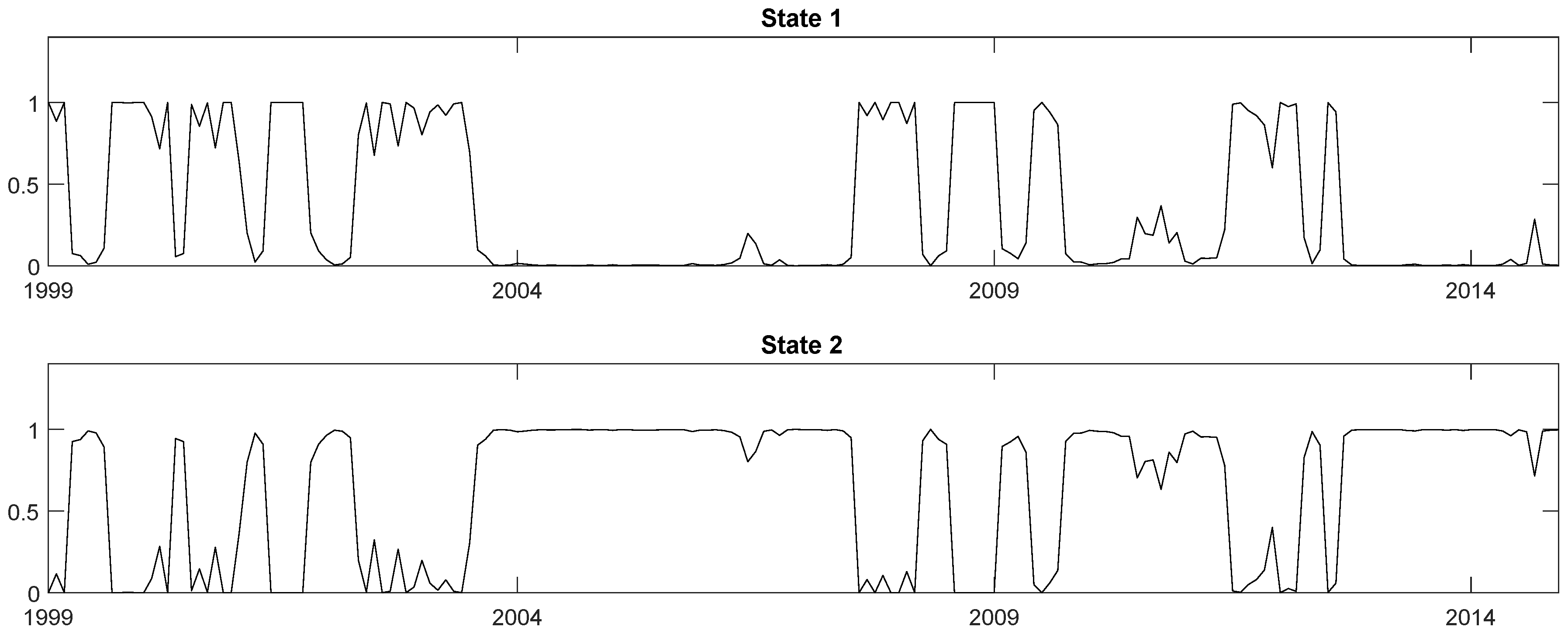
In Figure 2, the smoothed state probabilities of the VECM(1)-MSH(2) model are presented. They show that the two volatility regimes change frequently throughout the sample period so that guessing the change points reliably would be difficult for a researcher. Hence, using a model which allows for endogenously assigned volatility changes is clearly an advantage over a model where the volatility states have to be prespecified by the researcher.

To explore the identification issue, we have to consider the diagonal elements of ${\Lambda }_2$, which represent the variances of the structural shocks in the second volatility state relative to the first state, as explained in Section 3. They are displayed in

Table 5. Estimated relative variances of VECM(1)-MSH(2) model for $y_t={(q_t,p_t,c_t,s_t,r_t)}^{\prime }$.

Relative Variance	Estimate	Estimated Standard Error
${\lambda }_{21}$	1.557	0.587
${\lambda }_{22}$	0.765	0.294
${\lambda }_{23}$	0.479	0.186
${\lambda }_{24}$	0.024	0.007
${\lambda }_{25}$	0.202	0.075

, together with estimated standard errors. Four of the five estimated relative variances of the structural shocks in the second state are smaller than 1. Hence, most structural shocks have smaller variance in the second than in the first state. In other words, the second state captures potentially periods of lower volatility. From Figure 2, it can be seen that the first regime is associated with the period around the turn of the millennium, where the internet bubble burst, and with the period 2008/2009, where the financial crisis started. These events may have generated higher volatility in some of the structural shocks. Note, however, that at this point it is difficult to associate any of the shocks identified through heteroscedasticity with economic shocks of interest because the ordering of the shocks is arbitrary. Therefore, it is difficult to argue that specific economic shocks are more volatile in state 1.

For the identification of the shocks through heteroscedasticity, the diagonal elements of ${\Lambda }_2$ have to be distinct. Although the estimated diagonal elements are all distinct, the estimation uncertainty reflected in the standard errors is rather high and, hence, the true underlying quantities may not be distinct. This uncertainty in the estimates is not surprising given the relatively small sample size. However, some of the standard errors are quite small compared to the corresponding estimates of the relative variances, so it is reasonable to assume that at least some of the diagonal elements of ${\Lambda }_2$ are distinct. Thus, there is at least some identifying information in the second moments which may be sufficient to discriminate between competing conventional identification schemes. We emphasise that for this to hold, it is not necessary that all the ${\lambda }_{2i}$ are distinct.

We are primarily interested in a monetary policy shock and a stock market shock. Therefore, we place these shocks in the last two positions of ${\epsilon }_t$, that is, ${\epsilon }_t={({\epsilon }_{1t},{\epsilon }_{2t},{\epsilon }_{3t},{\epsilon }_t^{sm},{\epsilon }_t^{mp})}^{\prime }$. In other words, the stock market shock, ${\epsilon }_t^{sm}$, is the fourth shock, and the monetary policy shock, ${\epsilon }_t^{mp}$, is last. The other components of ${\epsilon }_t$ are left unspecified and represent other shocks to the economy.

We consider the two alternative identification schemes in

Table 6. Identification schemes for $y_t={(q_t,p_t,c_t,s_t,r_t)}^{\prime }$.

Scheme	B	$\mathbf{\Xi }\mathit{B}$
(1)	$\left[\begin{array}{ccccc}\ast & \ast & \ast & \ast & \ast \\ \ast & \ast & \ast & \ast \\ \ast & \ast & 0& \ast \\ \ast & \ast & \ast & \ast \\ \ast & \ast & \ast & \ast \end{array}\right]$	$\left[\begin{array}{ccccc}\ast & \ast & \ast & 0& 0\\ \ast & \ast & 0& 0\\ \ast & \ast & 0& 0\\ \ast & \ast & 0& 0\\ \ast & \ast & 0& 0\end{array}\right]$
(2)	$\left[\begin{array}{ccccc}\ast & 0& 0& 0& 0\\ \ast & 0& 0& 0\\ \ast & \ast & 0& 0\\ \ast & \ast & \ast & \ast \\ \ast & \ast & \ast & \ast \end{array}\right]$	$\left[\begin{array}{ccccc}\ast & \ast & \ast & \ast & \ast \\ \ast & \ast & \ast & \ast \\ \ast & \ast & \ast & \ast \\ \ast & \ast & \ast & 0\\ \ast & \ast & \ast & \ast \end{array}\right]$

. Since we have a cointegration rank $r=2$, the rank of $\Xi B$ is $K-r=3$. Thus, there can be two columns of zeros in the long-run effects matrix $\Xi B$. The first identification scheme in Table 6 assumes that both the stock market shock and the monetary policy shock are purely transitory and, hence, do not have any long-run effects on any of the variables. The two shocks are distinguished by the assumption that ${\epsilon }_t^{sm}$ does not affect the commodity price index instantaneously, but only with some delay. Hence, there is a corresponding zero in the third row of B. The long-run restrictions may be justified by the notion that the effects of monetary policy and stock market shocks should be transitory. In a conventional VAR analysis, effects of these shocks on the macroeconomic variables vanish over time (see Christiano et al. 1999; Bjørnland and Leitemo 2009). The restriction on the short-run effect is needed to distinguish the two shocks, which are both neutral in the long run, and it is part of the identification schemes used by Christiano et al. (1999), Bjørnland and Leitemo (2009), and others for US data. Note also that no restrictions are imposed on the first three columns of B and $\Xi B$ so that the first three shocks are identified purely by the volatility changes. Since we are not interested in them, we did not ensure that they have economic interpretations.

The second identification scheme is due to Bjørnland and Leitemo (2009), who used it for US data. They were also primarily interested in the last two shocks, and arbitrarily identified the first three shocks by imposing a recursive structure on their contemporaneous impact effects, which is seen by the recursive structure of the zero entries in the first three columns of B. Again, the last shock is specified as monetary policy shock. It is assumed to have no long-run impact on stock prices, and this distinguishes the shock from the stock market shock. Both shocks are assumed to have no impact effects on industrial production, the price level, and the commodity price index. This assumption reflects the belief that these variables move slowly in response to ${\epsilon }_t^{sm}$ and ${\epsilon }_t^{mp}$. There are no further long-run restrictions.

The two identification schemes differ not only in the way they identify the shocks of interest. While the first scheme relies primarily on long-run restrictions, the second scheme imposes most restrictions on the impact effects. Without heteroscedasticity, Scheme (1) is under-identified and the second scheme is just-identified. Thus, in the absence of heteroscedasticity, they cannot be compared with statistical tests without further assumptions. However, assuming that the shocks are already identified by the second-moment structure, the zero restrictions on B and $\Xi B$ are over-identifying and can be tested by standard likelihood ratio (LR) tests.

The results of such tests are presented in

Table 7. Tests of identification schemes.

${\mathbb{H}}_{\mathbf{0}}$	LR Statistic	Degrees of Freedom	p-Value
Scheme (1)	62.494	7	$4.787\times {10}^{-11}$
Scheme (2)	18.807	10	0.043

, where the alternative is a model that is purely identified by heteroscedasticity and has no zero restrictions on B or $\Xi B$. In addition to the value of the LR statistic, the assumed degrees of freedom of the ${\chi }^2$ limiting distributions are presented on which the p-values are based. For both tests, the number of degrees of freedom is determined under the assumption that the structural matrix B is fully identified by heteroscedasticity. The number of degrees of freedom for testing Scheme (1) is 7 because, for $r=2$, the long-run effects matrix $\Xi B$ has rank $K-r=3$ and, hence, each column of zeros counts for three independent restrictions only. In other words, the columns of the matrix $\Xi B$ can be represented as a linear combination of three basis vectors. A zero column is obtained if the basis vectors are multiplied by zero coefficients. Thus, each of the two columns of zeros is obtained by restricting the three weights of the basis vectors to zero. Hence, the 10 zero coefficients in the last two columns of the long-run effects matrix in Scheme (1) count for six restrictions only. In addition, there is one zero restriction on the impact effects matrix B.

For Scheme (1), the p-value of the LR test is less than 1%, so Scheme (1) is rejected at any conventional significance level. This also indicates that there must be identifying information in the second-moment structure because the ${\mathbb{H}}_0$ model is not identified by the zero restrictions alone. Thus, the heteroscedastic structure has identifying power. However, since the evidence of all relative variances being distinct in Table 5 is weak, there is of course the possibility that the structure is only partially identified by heteroscedasticity. In that case, the degrees of freedom of the LR tests in Table 7 may be smaller than assumed in the table, implying that the p-values would be even smaller than those in the table.

Considering the second p-value in Table 7, Identification Scheme (2) cannot be rejected at a 1% level, although its p-value is slightly below 5%, at least if a ${\chi }^2$ distribution with 10 degrees of freedom is used as reference. This outcome is interesting because, in a related study based on identification through heteroscedasticity, Lütkepohl and Netšunajev (2017a) found strong evidence against the restrictions for the US. Admittedly, this evidence is based on a quite different sample period. Moreover, Bertsche and Braun (2018) did not confirm this result with a different volatility model. However, Lütkepohl and Netšunajev (2017b) also found an implausible reaction of the inflation rate to a monetary policy shock for the US. Thus, it is instructive to see the responses of the variables to the two shocks of interest for our European model when Identification Scheme (2) is used.

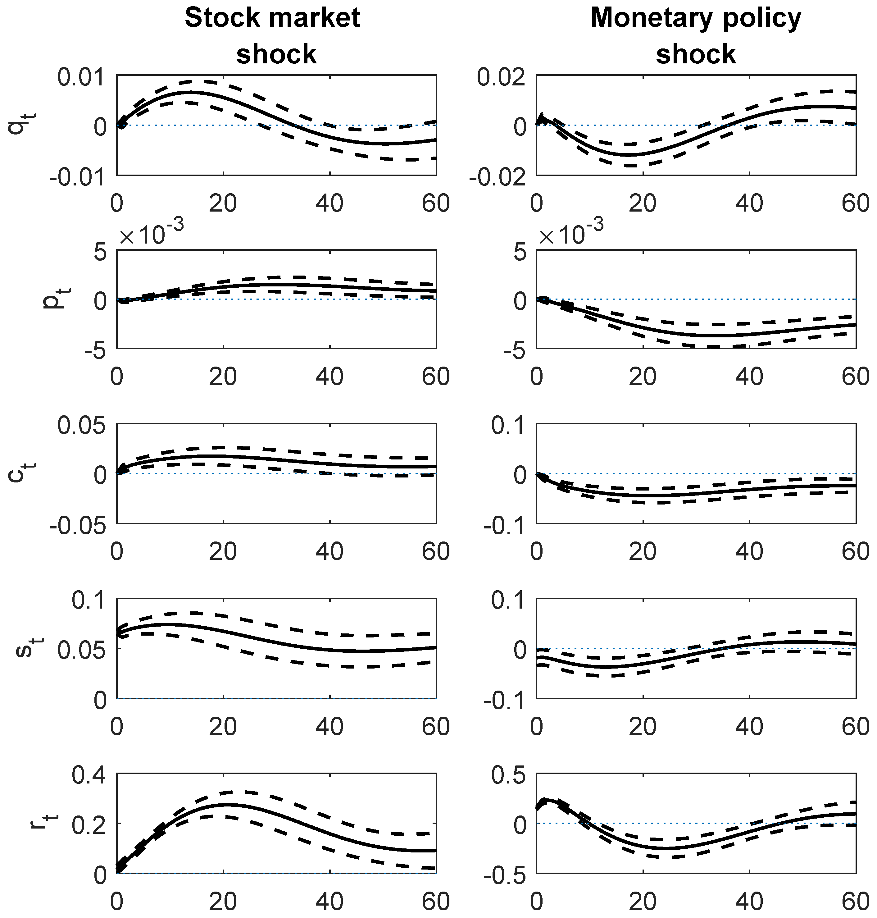
The estimated impulse responses with ± one standard error bootstrap confidence intervals are shown in Figure 3. The confidence intervals have a 68% level in a Gaussian environment. The standard errors are estimated with a fixed-design wild bootstrap conditioning on the transition probabilities, as proposed in Herwartz and Lütkepohl (2014) and also used in Lütkepohl and Netšunajev (2017a).

The responses of the variables to both shocks are quite plausible. A stock market shock is followed by increases in all other variables, although these upswings occur with some delay. This is in line with the studies by Bjørnland and Leitemo (2009) and Li et al. (2010) for the US. The increase in output and inflation is consistent with the view that a rise in stock prices increases consumption (Beaudry and Portier 2006) through a wealth effect and investment through a Tobin Q effect, thus inducing aggregate demand to increase. Due to nominal rigidities, prices react slowly, and inflation as well as commodity prices rise in the intermediate run. The response of the interest rate may be explained by the behaviour of an inflation-targeting central bank which is increasing interest rates to combat the inflationary pressure of a high aggregate demand.

A contractionary monetary policy shock, induced by an increase in the interest rate, reduces industrial production, the price level, and commodity prices with some delay. Similar to Peersman and Smets (2001) and Ehrmann et al. (2003), we do not find any price puzzle and observe long-run effects on prices. The shock leads to a long-lasting downturn of the stock index after a monetary policy tightening. This is in line with results of Bjørnland and Leitemo (2009) for the US, but the effect for the euro area is not as pronounced as in their study. Even though there is mixed evidence regarding the influence of monetary policy on industry- or country-level stock returns in Europe, most of the studies agree on a negative relation between ECB monetary policy and aggregate stock returns in the euro area (Kholodilin et al. 2009; Alessi and Kerssenfischer 2016; Fausch and Sigonius 2018). Clearly, our results support those previous findings which show that the policy of the ECB has a substantial impact on the stock market in Europe.

5. Conclusions

We have constructed a five-dimensional cointegrated structural VAR model for monthly euro area variables for the period 1999M1–2014M12 to study the relation between monetary policy and the stock market. The period of quantitative easing is explicitly excluded because it may be regarded as a new monetary policy regime. We allowed for conditional heteroscedasticity in the data and modelled volatility changes by a Markov-switching mechanism. Heteroscedasticity was used to disentangle a stock market and a monetary policy shock. Conventional identification restrictions on the impact and long-run effects of the structural shocks that have been used for a similar model for the US are found to be roughly consistent with the second-moment structure of the variables for our sample period, while an alternative identification scheme is strongly rejected.

The impulse responses for the maintained identification scheme are economically plausible and, in particular, production and price level go down after a contractionary monetary policy shock. Although the long-run impact of a monetary policy shock on stock prices is restricted to be neutral, such a shock is found to have a rather long-lasting negative impact on the stock market.

References

- Alessi, Lucia, and Mark Kerssenfischer. 2016. The Response of Asset Prices to Monetary Policy Shocks: Stronger Than Thought. Working Paper Series 1967; Frankfurt am Main, Germany: European Central Bank. [Google Scholar]
- Beaudry, Paul, and Franck Portier. 2006. Stock prices, news, and economic fluctuations. American Economic Review 96: 1293–307. [Google Scholar] [CrossRef]
- Bertsche, Dominik, and Robin Braun. 2018. Identification of Structural Vector Autoregressions by Stochastic Volatility. Technical Report 2018-01. Konstanz: University of Konstanz. [Google Scholar]
- Bjørnland, Hilde C., and Kai Leitemo. 2009. Identifying the interdependence between US monetary policy and the stock market. Journal of Monetary Economics 56: 275–82. [Google Scholar] [CrossRef]
- Blanchard, Olivier J., and Danny Quah. 1989. The dynamic effects of aggregate demand and supply disturbances. American Economic Review 79: 655–73. [Google Scholar]
- Bredin, Don, Stuart Hyde, Dirk Nitzsche, and Gerard O’Reilly. 2009. European monetary policy surprises: The aggregate and sectoral stock market response. International Journal of Finance & Economics 14: 156–71. [Google Scholar] [CrossRef]
- Cassola, Nuno, and Claudio Morana. 2004. Monetary policy and the stock market in the euro area. Journal of Policy Modeling 26: 387–99. [Google Scholar] [CrossRef]
- Cavaliere, Giuseppe, Anders Rahbek, and A. M. Robert Taylor. 2010. Cointegration rank testing under conditional heteroskedasticity. Econometric Theory 26: 1719–60. [Google Scholar] [CrossRef]
- Cavaliere, Giuseppe, Luca De Angelis, Anders Rahbek, and AM Robert Taylor. 2018. Determining the cointegration rank in heteroskedastic VAR models of unknown order. Econometric Theory 34: 349–82. [Google Scholar] [CrossRef]
- Christiano, Lawrence J., Martin Eichenbaum, and Charles L. Evans. 1999. Monetary policy shocks: What have we learned and to what end? In Handbook of Macroeconomics. Amsterdam: Elsevier, chp. 2. vol. 1, pp. 65–148. [Google Scholar] [CrossRef]
- Ehrmann, Michael, Leonardo Gambacorta, Jorge Martinez-Pagés, Patrick Sevestre, and Andreas Worms. 2003. The effects of monetary policy in the euro area. Oxford Review of Economic Policy 19: 58–72. [Google Scholar] [CrossRef]
- Fausch, Jürg, and Markus Sigonius. 2018. The impact of ECB monetary policy surprises on the German stock market. Journal of Macroeconomics 55: 46–63. [Google Scholar] [CrossRef]
- Fisher, Lance A., and Hyeon-Seung Huh. 2014. Identification methods in vector-error correction models: Equivalence results. Journal of Economic Surveys 28: 1–16. [Google Scholar] [CrossRef]
- Fisher, Lance A., Hyeon-Seung Huh, and Peter M. Summers. 2000. Structural identification of permanent shocks in VEC models: A generalization. Journal of Macroeconomics 22: 53–68. [Google Scholar] [CrossRef]
- Gonzalo, Jesus, and Serena Ng. 2001. A systematic framework for analyzing the dynamic effects of permanent and transitory shocks. Journal of Economic Dynamics and Control 25: 1527–46. [Google Scholar] [CrossRef] [Green Version]
- Haitsma, Reinder, Deren Unalmis, and Jakob de Haan. 2016. The impact of the ECB’s conventional and unconventional monetary policies on stock markets. Journal of Macroeconomics 48: 101–16. [Google Scholar] [CrossRef]
- Herwartz, Helmut, and Helmut Lütkepohl. 2014. Structural vector autoregressions with Markov switching: Combining conventional with statistical identification of shocks. Journal of Econometrics 183: 104–16. [Google Scholar] [CrossRef]
- Johansen, Søren, and Katarina Juselius. 1990. Maximum likelihood estimation and inference on cointegration—With applications to the demand for money. Oxford Bulletin of Economics and Statistics 52: 169–210. [Google Scholar] [CrossRef]
- Johansen, Søren. 1991. Estimation and hypothesis testing of cointegration vectors in Gaussian vector autoregressive models. Econometrica 59: 1551–81. [Google Scholar] [CrossRef]
- Johansen, Søren. 1995. Likelihood-based Inference in Cointegrated Vector Autoregressive Models. Oxford: Oxford University Press. [Google Scholar]
- Juselius, Katarina. 2006. The Cointegrated VAR Model: Methodology and Applications. Oxford: Oxford University Press. [Google Scholar]
- Kholodilin, Konstantin, Alberto Montagnoli, Oreste Napolitano, and Boriss Siliverstovs. 2009. Assessing the impact of the ECB’s monetary policy on the stock markets: A sectoral view. Economics Letters 105: 211–13. [Google Scholar] [CrossRef]
- Kilian, Lutz, and Helmut Lütkepohl. 2017. Structural Vector Autoregressive Analysis. Cambridge: Cambridge University Press. [Google Scholar]
- King, Robert, Charles I. Plosser, James H. Stock, and Mark W. Watson. 1991. Stochastic trends and economic fluctuations. American Economic Review 81: 819–40. [Google Scholar]
- Krolzig, Hans-Martin. 1997. Markov-Switching Vector Autoregressions: Modelling, Statistical Inference, and Application to Business Cycle Analysis. Berlin: Springer. [Google Scholar]
- Lütkepohl, Helmut, and Aleksei Netšunajev. 2017a. Structural vector autoregressions with heteroskedasticy: A review of different volatility models. Econometrics and Statistics 1: 2–18. [Google Scholar] [CrossRef]
- Lütkepohl, Helmut, and Aleksei Netšunajev. 2017b. Structural vector autoregressions with smooth transition in variances. Journal of Economic Dynamics and Control 84: 43–57. [Google Scholar] [CrossRef]
- Lütkepohl, Helmut, and Anton Velinov. 2016. Structural vector autoregressions: Checking identifying long-run restrictions via heteroskedasticity. Journal of Economic Surveys 30: 377–92. [Google Scholar] [CrossRef]
- Lütkepohl, Helmut. 2005. New Introduction to Multiple Time Series Analysis. Berlin: Springer. [Google Scholar]
- Lanne, Markku, Helmut Lütkepohl, and Katarzyna Maciejowska. 2010. Structural vector autoregressions with Markov switching. Journal of Economic Dynamics and Control 34: 121–31. [Google Scholar] [CrossRef]
- Li, Yun Daisy, Talan B. Iscan, and Kuan Xu. 2010. The impact of monetary policy shocks on stock prices: Evidence from Canada and the United States. Journal of International Money and Finance 29: 876–96. [Google Scholar] [CrossRef]
- Pagan, Adrian R., and M. Hashem Pesaran. 2008. Econometric analysis of structural systems with permanent and transitory shocks. Journal of Economic Dynamics and Control 32: 3376–95. [Google Scholar] [CrossRef]
- Peersman, Gert, and Frank Smets. 2001. The Monetary Transmission Mechanism in the Euro Area: More Evidence from VAR Analysis. Working Paper Series 0091; Frankfurt am Main, Germany: European Central Bank. [Google Scholar]
- Rigobon, Roberto, and Brian Sack. 2004. The impact of monetary policy on asset prices. Journal of Monetary Economics 51: 1553–75. [Google Scholar] [CrossRef]