Detecting and Measuring Nonlinearity

EconomiX-CNRS (UMR7235), Bureau G-517, Université Paris Nanterre, 92000 Nanterre, France
Econometrics 2018, 6(3), 37; https://0-doi-org.brum.beds.ac.uk/10.3390/econometrics6030037
Submission received: 28 January 2018
/
Revised: 18 March 2018
/
Accepted: 2 August 2018
/
Published: 9 August 2018
Abstract
:This paper proposes an approach to measure the extent of nonlinearity of the exposure of a financial asset to a given risk factor. The proposed measure exploits the decomposition of a conditional expectation into its linear and nonlinear components. We illustrate the method with the measurement of the degree of nonlinearity of a European style option with respect to the underlying asset. Next, we use the method to identify the empirical patterns of the return-risk trade-off on the SP500. The results are strongly supportive of a nonlinear relationship between expected return and expected volatility. The data seem to be driven by two regimes: one regime with a positive return-risk trade-off and one with a negative trade-off.
JEL Classification:
C10; G101. Introduction
Economic theories are often operationalized under linearity assumptions on the relationships between the underlying variables or joint normality assumptions on their distributions. Famous examples include the Capital Asset Pricing Model (CAPM) and Value at Risk models. Often, linearity and normality assumptions are needed in order to obtain analytical formulas and elegant characterizations of the phenomena of interest. However, such assumptions may lead to wrong conclusions when they are not valid. Recognizing these limits and observing the relatively high frequency of extreme economic events (e.g., financial crises and recessions), a body of the empirical literature in finance emphasizes the distributional characteristics of assets returns that do not reflect normality, in particular asymmetry and fat tails.
For example, Harvey and Siddique (1999, 2000) propose a model to estimate the conditional skewness and highlight the importance of taking this into account when analyzing the cross sectional properties of assets prices. Christoffersen et al. (2006) propose a framework to price options in the presence of conditional skewness. Feunou and Tedongap (2012) propose a stochastic volatility model with conditional skewness for assets prices and show that these distributional aspects are very important to explain how investors value options. Gabaix (2009, 2016) argues that stable laws approximate the distribution of many economic and financial variables fairly well while Gabaix (2011) proves that macroeconomic fluctuations can have granular origins. Indeed, Gabaix’s work draws attention on a more general issue, namely, the fact that the aggregation of independent phenomena does not always lead to the normal distribution as stipulated by the central limit theorem.
If non-normality is now well entrenched in the mind of academic researchers and financial risk managers, non-linearity has received much less attention in the literature. The joint normality of two random variables X and Y implies that is a linear function of X and that conversely is linear in Y. While a linear relation can still exist between X and Y without joint normality, a nonlinear relationship precludes joint normality. This shows that nonlinearity and non-normality are distinct concepts. Despite the availability of more and more complex computer solutions, linear relationships remain largely advocated for empirical inquiries in economics and finance. Prominent models that are based on linear relationships include the Arbitrage Pricing Theory (APT), Taylor rules and Keynesian consumption functions. Unfortunately, a linearity assumption may lead to wrongly falsifying a theory when the true unknown relationship of interest is nonlinear. Even after acknowledging that the relationship between two variables is nonlinear, finding the functional form that works best for the situation of interest may still be difficult.
In this paper, I propose an approach to measure the degree of nonlinearity of the relationship between two variables. For any pair , I define the exposure of Y to X as the expectation of Y given X. The relationship between X and Y is then said to be nonlinear if either Y is nonlinearly exposed to X or X is nonlinearly exposed to Y. Said differently, the relationship between X and Y is linear if and only if Y is linearly exposed to X and in turn X is linearly exposed to Y. Indeed, it is possible that be a linear function of X without being linear in Y. In this case, the linearity of is spurious as it is misleading about the true relationship between the two variables. Please note that the relationship between variables is approached in this paper from a predictive point of view rather than from a causal perspective. Knowing that the predictive relationship between X and Y is nonlinear is a good starting point for the search of the true underlying causal relationship.
The proposed measure for the degree of nonlinearity of the function , denoted , exploits the relative importance of the norms of the linear and nonlinear parts of in a functional space. The decomposition of into its linear and nonlinear part is done via a functional projection of onto a basis of orthogonal polynomials , where is a polynomial of order j and the orthogonality is defined with respect to a metrics . Upon observing that linear functions of X are loaded only on and , a function is said to be purely nonlinear when it is entirely loaded on the higher order polynomials . For any function of X, the value of always lies between 0 and 1, with 0 meaning that is linear in X and 1 meaning that is purely nonlinear as per the previous definition. The index is invariant to linear transformations of Y as well as to the addition of an independent noise to Y. It is not invariant to the choice of the metrics and it is therefore sensitive to transformations of X.
Unlike our proposed measure of nonlinearity, the Pearson linear correlation coefficient measures the propensity of a random variable Y of being replicated by a linear function of another variable X. It always lies between and , with 1 meaning a perfectly linear and positive relationship, 0 the absence of linear relationship and a perfectly linear and negative relationship. A linear correlation coefficient lying strictly between and 1 indicates that a fit of Y by a linear function of X will not be perfect. This imperfection arises either from the dependence of Y on random factors other than X or from nonlinearity in the relationship between Y and X (or both). The linear correlation coefficient is smaller than 1 in absolute value when X and Y are bound by a deterministic but nonlinear relationship. In an effort to repair the limitations of the linear correlation, measures of nonlinear association (typically, based on ranks) have been proposed. Notably, we have the rank correlation coefficient of Spearman (1904), Kendall’s tau (Kendall 1938, 1970), Goodman and Kruskal’s gamma (Goodman and Kruskal 1954, 1959) and the quadrant count ratio (see Holmes 2001). All rank correlation measures are designed to detect the strength of possibly nonlinear but monotonic relationships between Y and X. Unlike the linear correlation, a rank correlation coefficient equals 1 if for instance and if (assuming ). However, like the linear correlation, a rank correlation coefficient can be non significant if the relationship between X and Y is non-monotonic.
The remainder of the paper is organized as follows. Section 2 motivates the use of the nonlinearity index () proposed in this paper. Section 3 presents the derivation of . Section 4 discusses the choice of the metrics used to calculate . Section 5 examines the invariance properties of . Section 6 illustrates the calculation of for simple functions and warns against coarse errors when choosing the metrics . Section 7 proposes a feasible estimator for and shows its consistency. Section 8 proposes three applications of our methodology. In the first application, I compute the nonlinearity index of a European option relatively to the underlying asset. It is found that the degree of nonlinearity of the option depends on its maturity and strike as well as on the volatility of the underlying asset. The second application underscores the importance of performing a nonlinearity diagnosis prior to designing a hedging strategy for a portfolio. In the third application, I analyze the nature of the relationship between the returns on the SP500 index and the associated risk as measured by the realized variance (RV). The empirical results are supportive of the existence of a nonlinear relationship between the expected return and the expected risk. The SP500 seems to be driven by two regimes, one regime in which the expected return is increasing in the expected risk and another regime in which the trade-off is negative. Within each regime, the return-risk trade-off is approximately linear. Section 9 concludes. The mathematical proofs are gathered in Appendix A.
2. Motivation
This section starts with an empirical example which shows that can be linear with being concomitantly nonlinear. The second subsection presents a theoretical explanation for the empirical example. The third subsection presents a situation where ignoring the presence of nonlinearity in the data can be harmful.
2.1. Pitfalls in the Linearity of Conditional Expectations
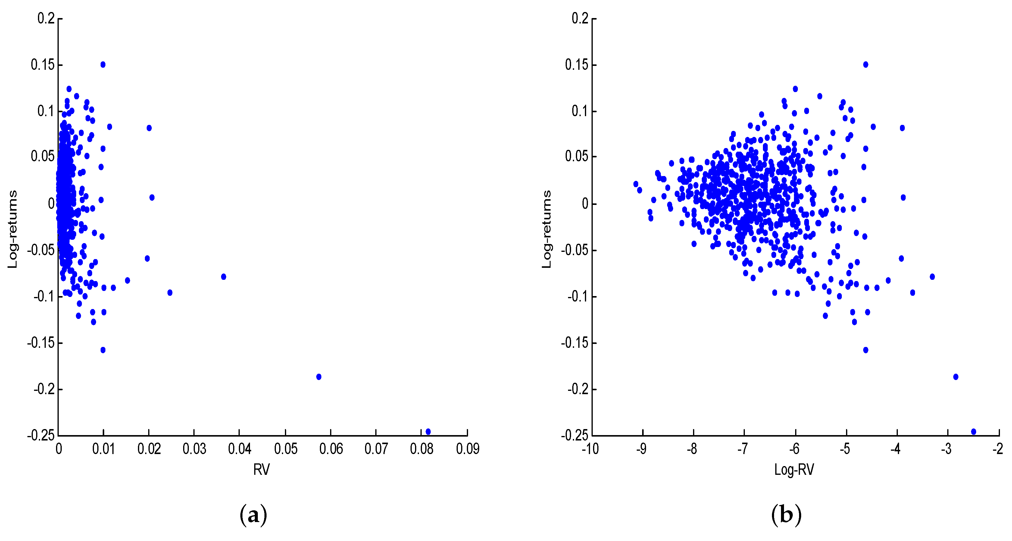
It is possible to have two random variables X and Y such that is linear in X while is nonlinear in Y. To support this point by empirical arguments, I downloaded daily observations on the SP500 from Yahoo Finance covering the period from 1 February 1959 to 30 April 2013 (14,173 days). The daily data are used to generate monthly returns () and log-returns denoted (652 months). The realized volatility () is computed as the sum of squared daily log-returns within Month t. Figure 1a shows the scatter plot of the on the y-axis against on the x-axis. The relationship between and is not visible on this plot. Figure 1b,c shows the scatter plots of against and respectively. Taking the log of zooms the pictures out. The shapes of the two graphs are quite similar.
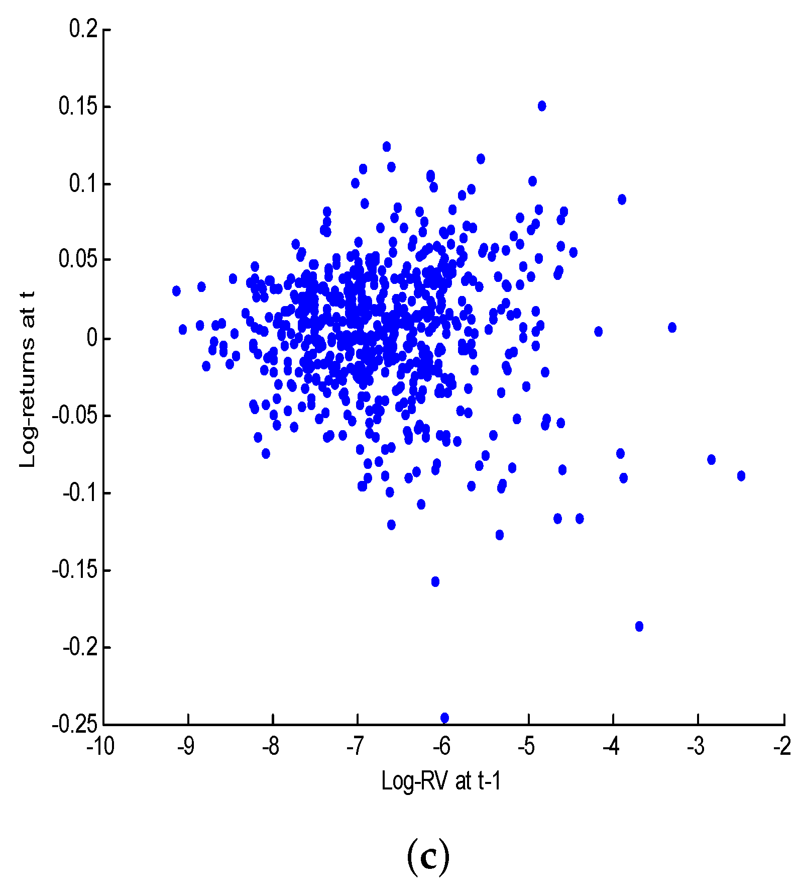
Figure 2 shows the nonparametric estimators of and . For any pair , the expectation of Y conditional on is estimated as:
where is the observed sample, is the Gaussian kernel, , and . The curve of shown on Figure 2a suggests that the relationship between and is more or less linear. However, the curve of shows on Figure 2b is clearly nonlinear.
The shape of is consistent with the existence of two regimes in the joint dynamics of , as found by Ghysels et al. (2014). The first regime is a vicious circle in which higher levels of expected risk are associated with higher losses (financial crises occur during this regime)1. By contrast, the second regime is a virtuous circle where higher levels of expected risk are associated with higher gains. The nonlinearity index proposed in this paper can be used to identify the two regimes.
2.2. Spurious Linearity
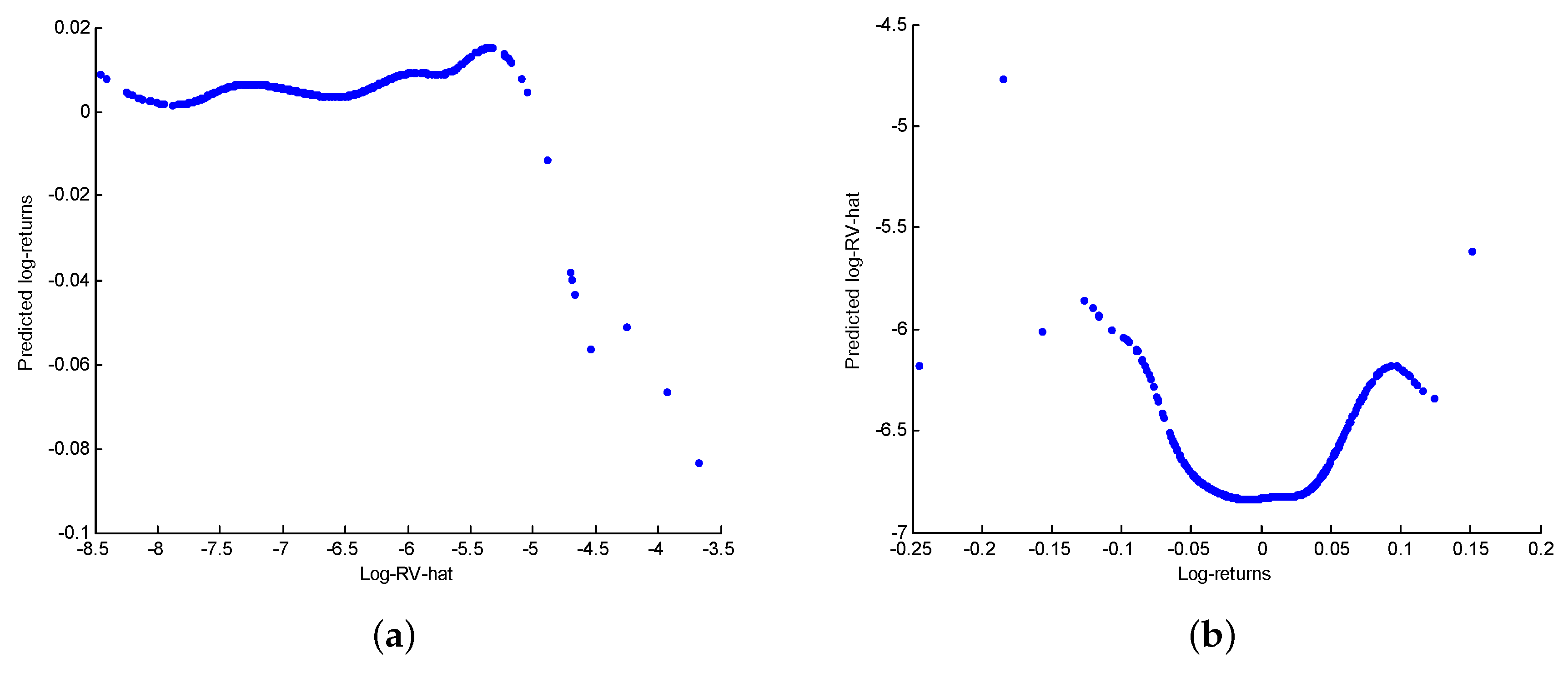
The expression “spurious linearity” may be used to describe a situation where the exposure of X to Y is linear while the reverse exposure is nonlinear, as in the previous example. To illustrate this concept theoretically, let us consider a deterministic mapping of the following form:
The relationship described by Equation (1) is plotted in Figure 3a. In this equation, Y is a deterministic and nonlinear transformation of X, which means that and that the pseudo- of the nonlinear regression of Y onto X is .2
However the reciprocal mapping from Y to X is not deterministic. To see this, assume that X follows a Uniform distribution on . Figure 3b plots X on the vertical axis against Y on the horizontal axis. Each value of Y is related to two possible values of X. Therefore, the knowledge of Y does not permit to identify with certainty the value of X to which it is associated. For each Y, the possible values of X are and .
To find , it helps to think of the joint distribution of as being generated by two regimes. Under Regime , and whereas under Regime , we have and . Hence:
This shows that is linear in Y while is nonlinear in Y. The pseudo- of the nonlinear regression of X onto Y is given by:
In summary, the exposure of Y to X is nonlinear and strong while the exposure of X to Y is linear and weak. This simply reflects the fact that X is a richer conditioning information set than Y. Indeed, the values of X implicitly determine the regimes so that:
where . Consequently, more information is gleaned about the type of relationship between X and Y by examining the expectation of Y given X.
The methodology proposed in this paper can be used to compute and compare the degrees of nonlinearity of and . If one of the two conditional expectations is far more nonlinear than the other, this would be suggestive that the relationship between X and Y is non-monotonic. In the empirical example of Figure 2b and the theoretical illustration of Figure 3a, an examination of the degree of nonlinearity of on increasing subsets of type of the support of X can be used to identify a candidate threshold for a piecewise linear approximation to the true model.
2.3. Disentangling Nonlinearity from Non-Normality
Models of equity premium prediction are typically specified as:
where is an excess return process, is a vector of risk factors and is an error term. The Capital Asset Pricing Model (CAPM) is a one factor model which takes to be the excess return on the market portfolio (See e.g., Sharpe 1964). Merton (1973) proposed an Intertemporal Capital Asset Pricing Model (ICAPM) where is the lagged realization of the asset’s volatility. Merton (1980) further insisted on the fact that empirical predictions of expected returns must be related to changes in expected future market risk in order to be consistent with equilibria model.
Following this idea, French et al. (1987) conducted an empirical study where and are respectively the stock market excess return and expected volatility. They found that expected return is positively related to expected risk while unexpected return is negatively related to unexpected risk (so-called “leverage effect”). Attempts have also been made to predict the equity premium using valuation ratios, such as companies’ sizes, earnings-to-price ratios, cash flow-to-price ratios, book-to-market equity, sales growth, etc. See for instance Fama and French (1996) and their famous three-factor model.
Another strand of this literature focuses on the estimation of long run return-risk trade-off. Using long horizon regression models, Bandi and Perron (2008) find that past realized market variance is a good predictor of future excess returns. Jacquier and Okou (2014) reappraise this result by separating the market realized variance into its continuous part and its jump component. They find that the power of past realized volatility at predicting the future risk premium is attributable to its continuous part. Okou and Jacquier (2016) refined their own results by performing statistical inferences on the term structure of the return-risk trade off at long horizon. Their main finding is that the results depend much on whether an intercept is included in the regressions or not, and that there is an horizon effect in the risk return trade-off. They argued that differences in the data frequency may be responsible for the conflicting empirical conclusions on the risk-return trade-off.3 I argue that in the presence of unsuspected nonlinearity, a linear regression can lead to quite misleading conclusions. In fact, the slope of the regression (2) can be insignificant as a result of being nonlinear in . Moreover, the estimate of that comes out of this regression is meaningless in the presence of nonlinearity.
Nonparametric regressions are sometimes advocated by empirical researchers on the ground that excess returns are non-normal (See e.g., Harvey 2001). However, it is easy to conceive a linear relationship between and with non-normal residuals. Likewise, can be nonlinear while is Gaussian. In the latter case, nonlinearity can cause the residuals of the linear regression of onto to be skewed or fat-tailed. The index proposed in this paper can help suspect whether the behavior of the model is driven by nonlinearity or non-normality.
3. Measuring Nonlinearity
Let the exposure of Y to X be given by:
where X and Y are scalar random variables and is a possibly nonlinear function of X. In assets pricing, Y could be the risk premium on an asset and X a measure of the risk for bearing that asset, in which case describes a nonlinear risk-return trade-off. Alternatively, Y can be viewed as an investors portfolio and X the traditional market index. In the latter case, would be reflecting a nonlinear exposure to the market stemming from a non-directional investment strategy. In macroeconomics, Y could be the inflation rate and X the unemployment rate, in which case features a nonlinear Phillips curve. Finally, could be an arbitrary process and its lagged value in a nonlinear time series model.
My objective is to assess the extent of nonlinearity of . Let the population linear regression of Y onto X be denoted by:
where and are real numbers. Please note that coincides with the linear regression of onto X and that coincides with if and only if Y can be represented as:
where is linearly uncorrelated with X. In the particular case where is bivariate Gaussian, and are necessarily identical and is normally distributed as well. That is, the joint Gaussianity of is sufficient but not necessary for linearity.
With no loss of generality, I assume that admits a series representation of the following form:
where is a complete sequence of orthogonal polynomials over the support of X under some metrics , that is:
and is the tight range of X, that is, the domain over which the values of X are meaningful. For instance, is a priori for a price process and for a log-return process. is a polynomial of order j and . Please note that satisfies (5) if and only if:
See Carrasco et al. (2007) and the references therein. Upon knowing , the metrics can always be selected to meet the condition (6).
Let the projection of onto under the metrics be given by:
where:
and denotes the scalar product under . The function is linear if and only if it is loaded only on the first two basis functions, that is:
where the first equality is deduced from (5) and the last equality stems from (4).
is nonlinear if and only if the residual of the projection of onto , i.e., , is not identically null. Therefore, the nonlinear part of may be isolated as:
Based of this observation, a measure of the degree of nonlinearity of is given by:
By construction, if is perfectly linear and if is fully loaded on the nonlinear basis functions. Hence, always lies between 0 and 1 and is decreasing in the degree of linearity of as measured by the ratio of the norms of and . Equivalent expressions of are therefore given by:
Please note that is not defined when , just as the linear correlation coefficient between Y and a constant does not exist.
The choice of the metrics is a crucial step of the methodology presented above. Indeed, the value of depends on the metrics used and a bad choice of metrics may lead to spuriously detect nonlinearity. This issue is discussed in the next section.
4. The Conditioning Information Set and the Suitable Choice of Metrics
Let denote the conditioning information set, that is, the support of X. A probability measure on is said to belong to Pearson’s family if and only if it satisfies:
For instance, letting and leads to:
which is the Gaussian probability distribution function on . Likewise, letting yields the uniform distribution on while setting () and yields an exponential distribution on . The Student, Gamma, Beta distributions are also special members of the Pearson family. See Johnson et al. (1994, pp. 15–25) and Bontemps and Meddahi (2012) for more details.
If a probability measure defined on belongs to the Pearson family, the sequence of orthogonal polynomials under are given by Rodrigues’ formula (see Askey 2005):
where is the nth order differentiation operator and is a sequence of normalization factors that could be chosen so as to achieve specific purposes. That is, any sequence given by (14) satisfies:
Subsequently, we consider five cases that are representative of the situations that researchers will often face in practice.
Case 1: When , a suitable choice of metrics is . The corresponding orthogonal basis is given by Hermite polynomials:
where is the derivative of with respect to x. In this case, the nonlinearity of is given by:
where:
Case 2: When , one may use along with the corresponding orthogonal basis formed by Laguerre polynomials:
The nonlinearity of is then given by:
where:
Case 3: If X can realistically not fall below a given threshold , one may consider defining the domain of X as . The corresponding Laguerre polynomials are obtained by noting that:
Hence for , is orthogonal to with respect to on .
Case 4: When , the simplest possible choice of metrics is uniform weighting function . The corresponding orthogonal basis of functions consists of Legendre’s polynomials:4
Case 5: For an arbitrary bounded domain , we simply note that:
Hence, by letting , it is straightforward to show that:
Hence, a suitable choice of basis functions when is given by the sequence . The measure of nonlinearity for this case is:
where:
The latter set up best suits for measuring nonlinearity on segments of the support of X.
Any metrics that follows the guideline described above will delivers a measure of nonlinearity that is reliable. This means that for an appropriately chosen metrics, the function under consideration is nonlinear as soon as is strictly positive. However, the interpretation of the result is “metrics specific”, meaning that is a relative measure of nonlinearity. While the degrees of nonlinearity of different functions obtained under different metrics cannot be compared, different functions sharing the same support can be compared under the same metrics.
5. Invariance Properties
Observe that has the flavor of the of a linear regression as it measures the “goodness-of-fit” of the functional projection of onto . Based on this observation, one is tempted to claim that shares all the invariance properties as an . However, such a statement is only partially true because of the dependence of on the metrics . The invariance properties of are discussed below.
Proposition 1.
κ is invariant to a linear transformation of Y.
Proposition 1 establishes that the amount of nonlinearity remains the same under drifting and scaling of Y. Applied to a portfolio of financial assets, this property means that leverage does not affect the nonlinearity of a financial position. Another property shared by the is stated below.
Proposition 2.
κ is invariant to the addition of a randomness ε to Y provided that ε is independent of X.
This property is rather interesting as it implies that may be used to diagnose linear models with additive error terms. Let us assume that X is the return on the market index and Y the return on the portfolio of an investor such that (i.e., we are assuming that the exposure of Y to X is perfectly linear). The strength of the exposure of Y to X is given by the linear correlation between Y and , that is, the square root of of the regression of Y onto X. Suppose the investor decides to implement a non-directional (i.e., market neutral) diversification strategy by changing Y into , where is independent of X. The exposure of the new position is given by , where and . The alpha of the new position may have increased of decreased depending on the value of and its beta is reduced by half. However, the nonlinearity of the new position as measured by is unaltered since remains linear in X.
The next proposition examines the consequence of an addition of a linear function of X to Y.
Proposition 3.
If Y is nonlinearly exposed to X, Adding a linear function of X to Y does not necessarily decrease its degree of nonlinearity.
Indeed, is not invariant to the addition of a linear function of X to Y. To understand this result in the context of the proposition (see the proof in Appendix A for more details), suppose is positive so that . Then adding to Y exacerbates its nonlinearity if a is negative and lies within the range . The degree of nonlinearity decreases only if or . Alternatively, suppose is negative so that . Then adding to Y exacerbates its nonlinearity if a is positive and lies within the range . Otherwise, the nonlinearity of Y decreases. Applied to portfolio choice, Proposition 3 implies that an asset that is linearly exposed to X can be used to increase the nonlinearity of an already nonlinear position Y. A sufficient condition for the addition of to reduce the nonlinearity of Y is that a be of the same sign as .
The property of highlighted by Proposition 3 is also shared by the linear correlation coefficient. Unlike the correlation coefficient however, the value of is sensitive to drifting and scaling of X.
Proposition 4.
Let where a and b are some constants. Then the degree of nonlinearity of Y with respect to X under is equal to its degree of nonlinearity with respect to Z under .
The result of Proposition 4 stems from the fact that any transformation of X alters the metrics , which in turn invalidates the orthogonality of . It implies that the values of are not directly comparable across different choices of metrics, which is a drawback of the proposed methodology. However, this drawback is a minor one if is continuous and puts zero weights outside the support of X. Also, functions that are defined on the same domain may be compared under the same metrics provided that they all have finite norms.
6. Spurious Nonlinearity
This section illustrates how to compute when is known and in passing, underscores the importance of selecting the metrics wisely. Indeed, spurious nonlinearity may arise from a bad choice of metrics. To see this, let us consider the exponential function , which also has the following representation:
It is tempting to claim based on (24) that . However, such a claim would be false since and have been defined as the coordinates of in the basis formed by the orthogonal polynomials . By noting that for the exponential function, we let so that , where are Hermite polynomials and:
This yields the following measure of nonlinearity:
Let us now consider . This function is defined only for and hence, its nonlinearity should not be measured as though x lies on the whole real line. For illustration purposes, let us ignore this warning by letting . This leads to:
The measure of nonlinearity that results is:
which is quite excessive compared to what is obtained for the exponential. In reality, the nonlinearity calculated above is for the function given by:
which is distinct from on . The domain of is the whole real line whereas the tight domain of is . This explains why we obtain a spuriously high value of .
Let us now account for the fact that the domain of is by letting , where are Laguerre polynomials. We obtain:
This yields:
which is more reasonable than previously.
7. Feasible Estimators
Upon observing a sample of size T from the joint distribution of , the conditional expectation can be estimated by the nonparametric method of Nadaraya (1964) and Watson (1964):
where is a kernel function and h is a bandwidth.
With the estimator above in hand, the sample counterpart of is:
where
with if , if and if . Given these choices of metrics, integrals of the form can be solved analytically when is a polynomial. For more complicated functions however, numerical quadratures should be used.
When , the quadrature rule yields:
where are Gauss-Hermite quadrature points associated with the weights .
For the alternative metrics , the quadrature rule becomes:
where are Gauss-Laguerre quadrature points associated with the weights .
Finally, for the natural metrics , we have:
where are Gauss-Legendre quadrature points associated with the weights .
The quadrature rules above are designed such that they are exact when the integrand is a polynomial of order . That is:
Thus, it is straightforward to show that:
where . If , the approximation error of by a quadrature rule is:
Please note that the finiteness of the norm of imposes that . Furthermore, is an approximation of . Consequently, the approximation error (42) converges to zero fast as N increases (especially for and ). This is a good news given that the expression of only requires on and .
The next proposition states a consistency result for by assuming that its numerical approximation error is negligible.
Proposition 5.
Assume that , where is a sequence of bandwidth satisfying as . Then we have:
According to Proposition 5, any consistent estimator of may be plugged into (30) to (32) to obtain a consistent estimator of . Nonparametric estimators of type (28) have been shown to be consistent under quite general settings (Bierens 1987).
8. Applications
This section presents three applications of . The first subsection discusses the degree of nonlinearity of a European option with respect to the underlying asset. The second subsection discusses the optimal hedge ratio in the presence of nonlinearity. The third subsection presents an empirical example where the relationship between the risk and the returns on the SP500 index is analyzed.
8.1. How Nonlinear Are Put and Call Options?
This section examine the nonlinearity of the price of a European style option with respect to the underlying asset. This exercise is trivial in a sense as options generate nonlinear payoffs by construction. However, it is nevertheless useful as it gives us a pretext to compare the degree of nonlinearity of several functions under the same metrics and to further illustrate the importance of correctly selecting the metrics .
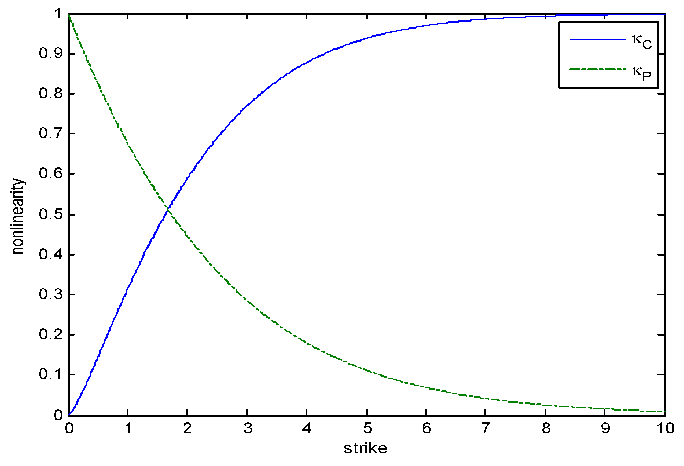
The payoff a European Call option at maturity is given by , where X is the price of the underlying asset and K is the strike.
If one ignores the fact that the support of X is and use to compute the nonlinearity of , then one obtains the following expressions:
where is the standard normal cumulative distribution function. This suggests that where , and are given above. Evaluating this formula at yields:
The value of is clearly misleading since is linear when .
To avoid spurious nonlinearity, one uses . We have:
Hence the nonlinearity of the payoff of an European Call is given by:
We see that the formula above now implies that , consistently with the fact that when .
I now consider the payoff a Put option with strike K, given by . Having learned from the previous example, I set and obtain:
The nonlinearity of the payoff of an European Put is given by:
Please note that for a Put, when . Hence, we expect to see as . Indeed, we have:
Figure 4 compares the nonlinearity of a the payoffs of a Call and a Put under the metrics . As K increases to infinity, starts at and converges to 1 whereas at and converges to zero .5
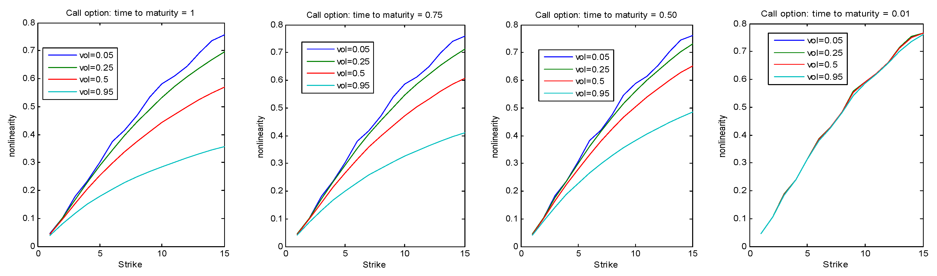
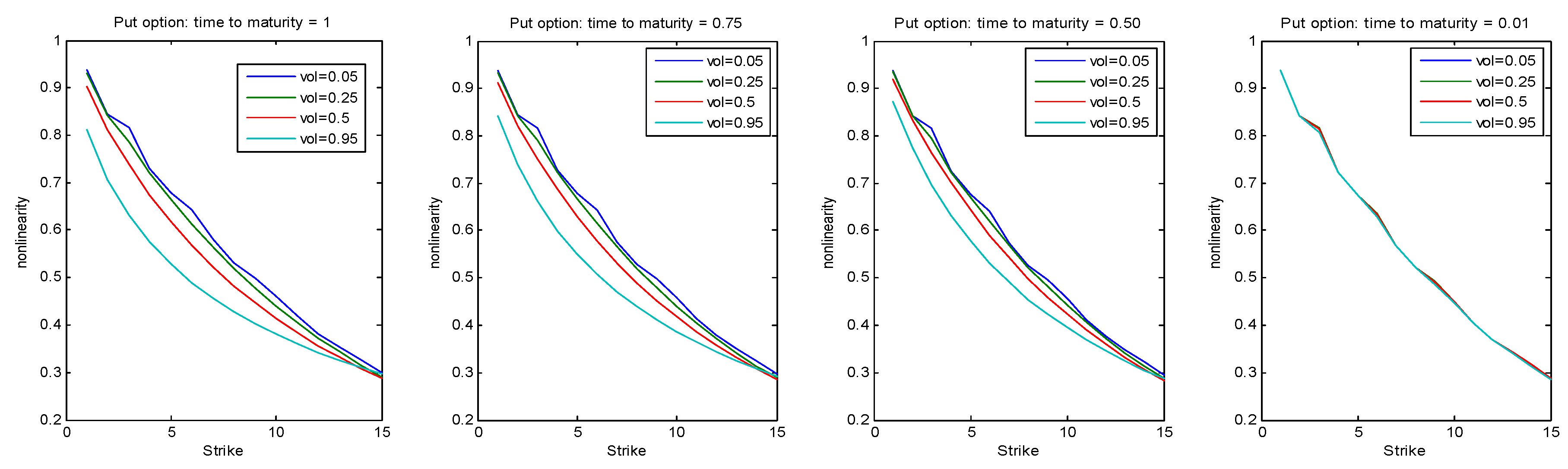
Over the course of its lifetime, the price of a Call as given by the Black-Scholes formula is:
where:
X is the price of the underlying asset, K is the strike, t is the current date, T is the maturity and is the spot volatility of X.
The following quantities are needed in order to evaluate the nonlinearity of as K, t and vary:
These integrals cannot be computed in closed form. A numerical approximation based on Gauss-Laguerre rule yields:
where are quadrature points associated with weights . Hence,
For an European Put option, the price evolves according to:
The nonlinearity of this price with respect to the underlying asset is:
Figure 5 is drawn by assuming that year, , and . For a Call option (resp., Put options), nonlinearity increases (resp., decreases) in the strike K for all values of volatility and time to maturity. For both types of options, the nonlinearity is decreasing in the volatility and time to maturity. The nonlinearity appears to be more sensitive in the volatility and time to maturity for a Call than for a Put.
8.2. Nonlinearity and Optimal Hedging
Assume that an investor wants to hold units of a risk free asset () and units of a risky asset () so as to hedge against the volatility of an asset . This investor would form a hedge portfolio whose value is . The hedging error is given by:
where
In practice, a perfect hedge that results in can rarely be achieved. Therefore, the best solution often consists of minimizing the variance of the hedging error with respect to the “hedge ratio” , which is the number of units of Asset to hold per unit of Asset . When is the payoff of an option and the price of the underlying asset, corresponds to the “delta” of the option (hence the expression “Delta Hedging”).
The optimal hedging problem boils down to the following minimization:
The optimal hedge ratio is given by . However, can be zero if is nonlinearly exposed to . In this case, one would wrongly conclude that Asset is of no help for hedging against the fluctuations of .
Now, suppose we have detected that is nonlinear using the methodology proposed in this paper. A reasonable hedging strategy would therefore consist of first using state-of-the-art models to predict as and next linearizing around this prediction to obtain:
An approximately optimal hedge ratio would then be given by:
This example underscores the importance of being aware of the presence of nonlinearity in assets returns for a sound portfolio risk management.
8.3. Empirical Application: Return-Risk Trade-Off on the SP500
In this section, I illustrate an empirical use of the measure of nonlinearity by performing an analysis of the return-risk trade-off based on the Merton’s (1973) intertemporal capital asset pricing model (ICAPM). This model posits the following relation between the conditional expected return on the market index and the conditional expected variance :
where is the risk free rate and is the relative risk aversion coefficient of the representative agent. A multivariate version of the ICAPM is proposed in Bollerslev et al. (1988).
Ghysels et al. (2005) employed a MIxed DAta Sampling (MIDAS) methodology to the CRSP value-weighted portfolio and concluded that “there is a [positive] risk-return trade-off after all.” Previous studies who found a positive relationship between risk premium and expected risk include French et al. (1987) and Campbell and Hentschel (1992), in contrast with Nelson (1991) who find a negative relationship or Glosten et al. (1993) and Harvey (2001) whose conclusions are mixed. Ghysels et al. (2005) attributes the conflicting conclusions to differences in the models posited for the conditional variance. Jacquier and Okou (2014) suspect the differences in data frequencies to be responsible of the inconsistencies across findings. The empirical results of the current paper suggest that the controversy on the nature of the return-risk trade-off is mainly due to nonlinearity.
I consider estimating the following nonlinear version of the ICAPM:
If one assume that and are IID and Gaussian, Equations (54) and (55) imply that:
As in the ICAPM, the conditional expected return is increasing in conditional expected variance . Unlike in the ICAPM, the relationship between the conditional expected return and the innovation on the log-variance process () is explicitly characterized. Namely, the conditional expected return is decreasing in the variance of , as observed empirically by French et al. (1987). Finally, the market price of risk is a nonlinear function of the conditional expected variance.
I estimate the AR(1) for the log-RV and compute the fitted values as . These fitted values are the expected risk at time t as perceived by investors at time . The estimated coefficients are (significant at level) and (significant at level). The of this regression is and the estimated error variance is . Figure 5a shows the scatter plot of against . Next, I regress the log-return on and a constant and compute the fitted values as . This yields and . Neither of these coefficients is significant at level and not surprisingly, the of the regression is less than . The poor fit provided but the linear regression of onto suggests that the relationship between these variable is nonlinear. This is confirmed by the nonparametric estimator of shown by Figure 2.
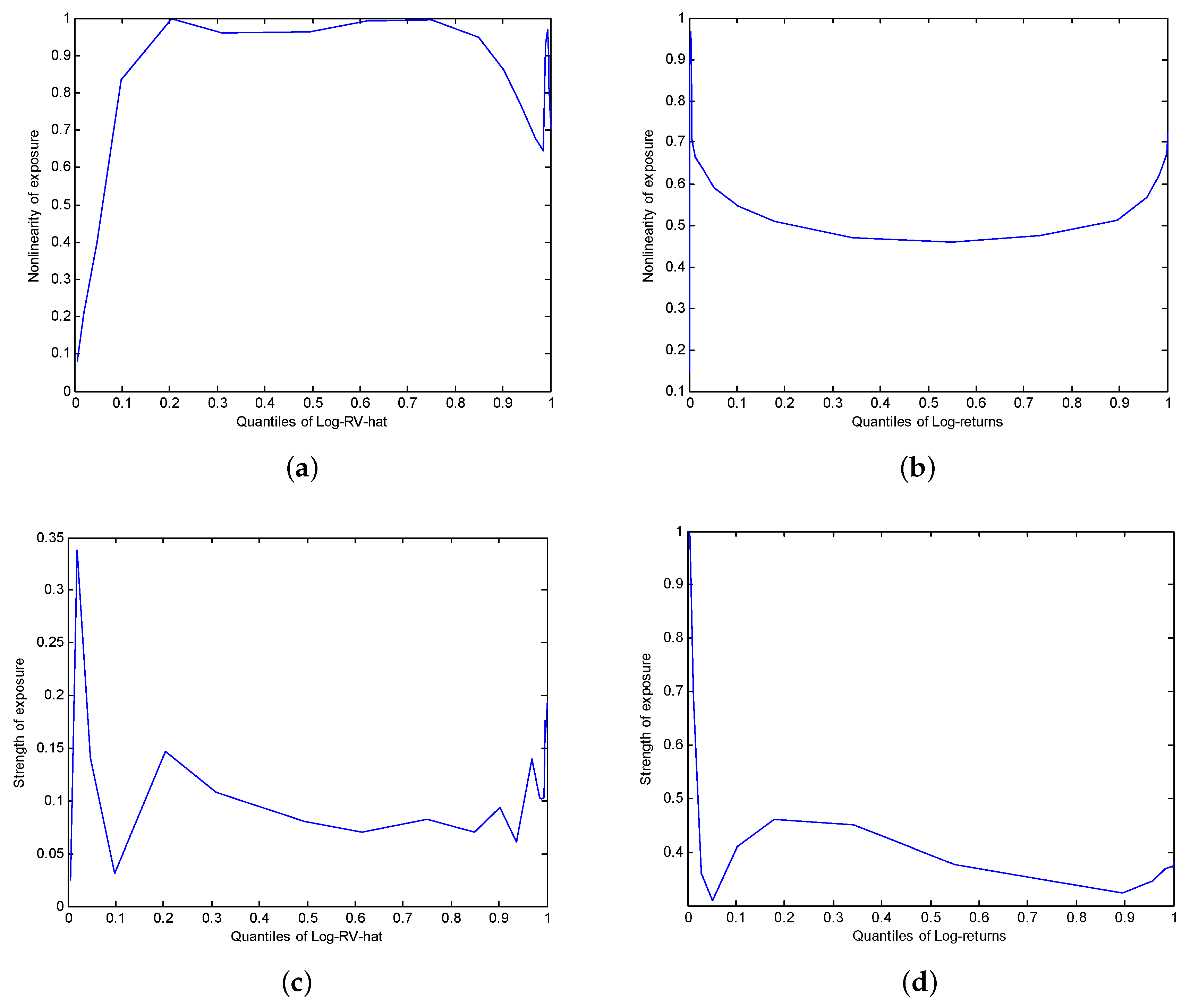
Figure 6a,b respectively show the estimated nonlinearity of and on increasing segments of the support of and . The scaling of the x-axis corresponds to the quantiles of the conditioning variable. For any pair , the nonlinearity of is computed on the segments using the metrics along with Gauss-Legendre’s polynomials, where:
For each , is obtained by spline interpolation based on .
We see that the nonlinearity of increases fast and remains high after the 20th percentile of . By contrast, the nonlinearity of decreased on the first portion of the support of and increases steadily after the median. The point at which the nonlinearity of is minimized, , is a good candidate for the threshold of a piecewise linear model.
Figure 6c,d respectively show the strength of the exposure of to and to on increasing subsample of type . The correlation of and approximately equals on a large portion of the support of while that of and is on average equal to . This means that fits better than fits .
Acting on the fact that the linearity of reaches its maximum at , I estimate the following piecewise linear regression:
Let denote the fitted values obtained from this piecewise linear regression.
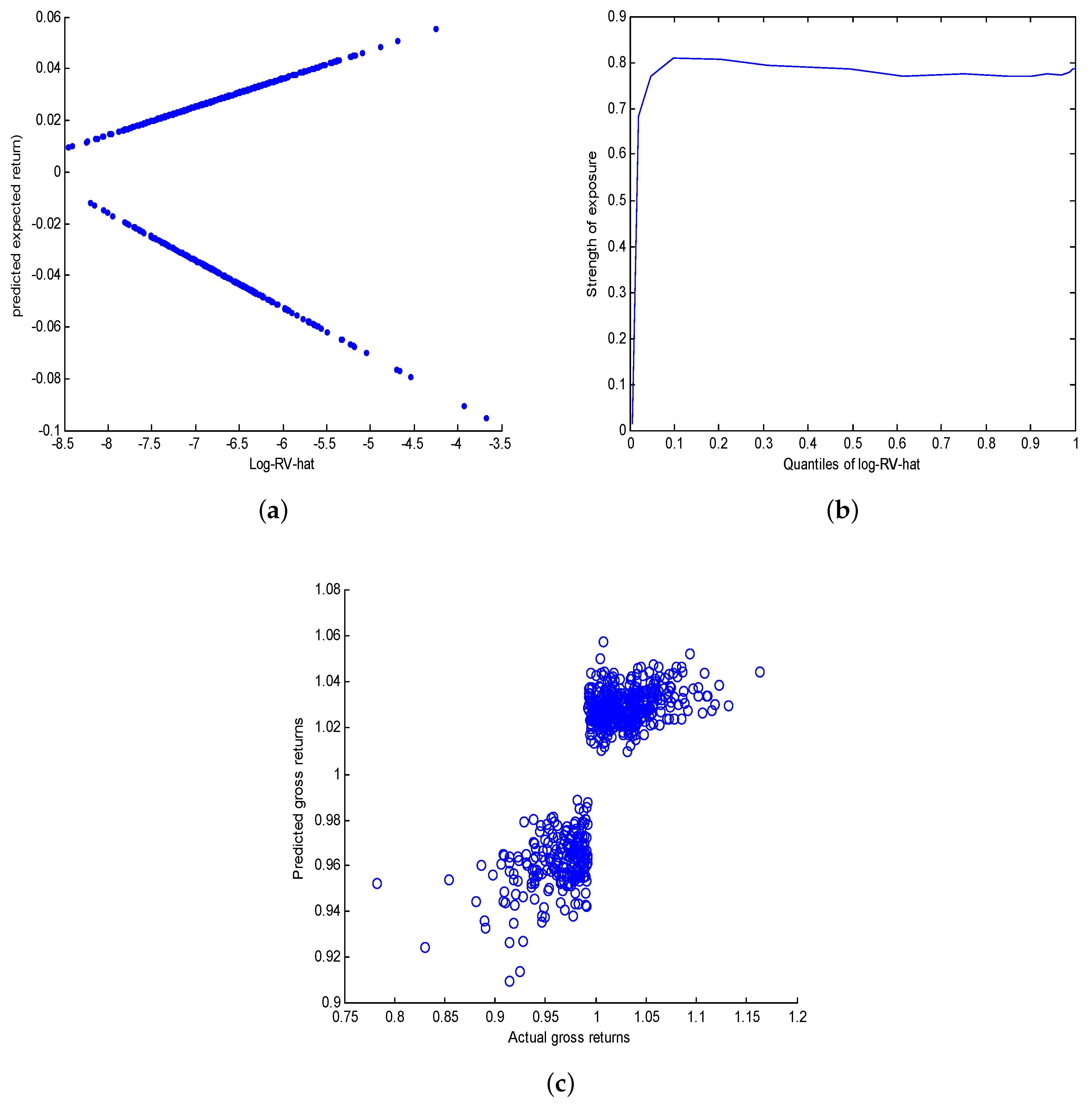
Figure 7a shows the fitted regression lines while Figure 7b plots the linear correlation between and against the quantiles of . The correlation between and reaches at the 10th percentile and remains above thereafter. This strong nonlinear relationship between log-returns and log-realized volatility is completely missed by the naive linear regression of onto .
The estimated regression lines are:
The estimated error variances are respectively for the first regime and for the second regime. Finally, the estimated nonlinear return-risk trade-offs are:
Based on the equation, the unconditional correlation between the actual gross-returns and their predictions shown on Figure 7c is .
A natural implication of these results is that option pricing models should at least account for the presence of regimes or parameter uncertainty in the distribution of the returns on the underlying asset. Our findings provide a strong empirical support for regime switching models in which volatility influences returns (as in Duan et al. 2002), heteroskedastic mixture models or Bayesian models that naturally account for parameter uncertainty (e.g., Rombouts and Stentoft 2014, 2015).
9. Conclusions
This paper proposes an approach to measure the degree of nonlinearity of the exposure of a variable Y to the movements of another variable X. The exposure is defined in terms of the expectation of Y conditional on X, denoted . The proposed measure of nonlinearity, denoted , is constructed by exploiting the ratio of the norms of the linear and nonlinear parts of . The separation of into its linear and nonlinear parts is done via its projection onto an orthogonal basis of polynomials with respect to some metrics . The invariance properties of are studied. For cases where the exposure function is unknown, an estimator of that exploits a consistent nonparametric estimator is proposed. It is shown that inherits the consistency of .
Three fields of application are proposed. The first application concerns the measurement of the nonlinearity of the price of a European style option with respect to the underlying asset. I find that the nonlinearity of a Call increases with the strike but decreases with the volatility and time to maturity. For a Put, the nonlinearity decreased with the strike, volatility and time to maturity. The second application attempts to motivate the use of for portfolio risk management. Basically, I argue that hedge ratios are misleading in the presence of nonlinearity and therefore, that a diagnosis of nonlinearity should be performed prior to designing the optimal hedge strategy. The third application is empirical and concerns the relationship between the return and realized volatility of the SP500 index. The empirical results provide supportive evidence that the return-risk trade-off on the SP500 is nonlinear and governed by regimes.
Acknowledgments
The author wishes to thank Marine Carrasco, Bruno Feunou, Pierre Evariste Nguimkeu, Georges Tsafack, Romeo Tedongap, the Editor and two anonymous referees for helpful comments.
Conflicts of Interest
The author declares no conflict of interest.
Appendix A. Proofs of Propositions
Proof of Proposition 1.
Let where a and b are constants. We have:
where and for all . Hence:
This shows that and Y have the same amount of nonlinearity. □
Proof of Proposition 2.
Please note that , which has the same amount of nonlinearity as according to Proposition 1. □
Proof of Proposition 3.
implies , where and for all . Also, “Y is nonlinearly exposed to X” means that . We have,
where we note that . Taking the derivative of with respect to a yields:
Hence, is increasing in the region , and decreasing in the region . Furthermore, is symmetric around .6 Consequently:
where and
Proof of Proposition 4. First, note that:
Next, observe that is an orthogonal basis under . That is, for :
This shows that is an orthogonal basis under . The coordinates of in this basis is:
Furthermore, and hence:
The L.H.S. is the degree of nonlinearity of Y with respect to X under while the R.H.S. is its degree of nonlinearity with respect to Z under
Proof of Proposition 5.
Please note that where for all j. Hence:
where for all j. Let so that . We have:
Now, note that . Hence
The dominant term of this expression is and it satisfies:
This shows that . The same rate of convergence is obtained for by using Slutsky’s Theorem. For the term , we have:
so that
Finally, by Slutsky’s Theorem. □
References
- Askey, Richard. 2005. The 1839 paper on permutations: Its relation to the Rodrigues formula and further developments. In Mathematics and Social Utopias in France: Olinde Rodrigues and His Times. Edited by Simon Altmann and Eduardo. L. Ortiz. History and Mathematics 28. Providence: American Mathematical Society, pp. 105–18. [Google Scholar]
- Bandi, Federico M., and Benoit Perron. 2008. Long-Run Risk-Returns Trade-Offs. Journal of Econometrics 143: 349–74. [Google Scholar] [CrossRef]
- Bierens, Herman J. 1987. Kernel estimators of regression functions. In Advances in Econometrics 5th World Congress. Edited by Truman F. Bewley. Cambridge: Cambridge University Press, pp. 99–144. [Google Scholar]
- Bollerslev, Tim, Robert F. Engle, and Jeffrey M. Wooldridge. 1988. A Capital Asset Pricing Model with Time-Varying Covariances. Journal of Political Economy 96: 116–31. [Google Scholar] [CrossRef]
- Bontemps, Christian, and Nour Meddahi. 2012. Testing Distributional Assumptions: A GMM Approach. Journal of Applied Econometrics 27: 978–1012. [Google Scholar] [CrossRef]
- Campbell, John. Y., and Ludger Hentschel. 1992. No news is goodnews: An asymmetric model of changing volatility in stock returns. Journal of Financial Economics 31: 281–318. [Google Scholar] [CrossRef]
- Carrasco, Marine, Jean-Pierre Florens, and Eric Renault. 2007. Linear inverse problems and structural econometrics: Estimation based on spectral decomposition and regularization. Handbook of Econometrics 6: 5633–751. [Google Scholar]
- Christoffersen, Peter, Steve Heston, and Kris Jacobs. 2006. Option valuation with conditional skewness. Journal of Econometrics 131: 253–84. [Google Scholar]
- Duan, Jin-Chuan, Ivilina Popova, and Peter Ritchken. 2002. Option pricing under regime switching. Quantitative Finance 2: 1–17. [Google Scholar] [CrossRef]
- Fama, Eugene F., and Kenneth R. French. 1996. Multifactor Explanations of Asset Pricing Anomalies. The Journal of Finance 51: 55–84. [Google Scholar] [CrossRef] [Green Version]
- Feunou, Bruno, and Romeo Tedongap. 2012. A Stochastic Volatility Model with Conditional Skewness. The Journal of Business and Economic Statistics 30: 576–91. [Google Scholar] [CrossRef]
- French, Kenneth R., G. William Schwert, and Robert F. Stambaugh. 1987. Expected stock returns and volatility. Journal of Financial Economics 19: 3–29. [Google Scholar] [CrossRef]
- Gabaix, Xavier. 2016. Power Laws in Economics: An Introduction. Journal of Economic Perspectives 30: 185–206. [Google Scholar] [CrossRef]
- Gabaix, Xavier. 2011. The Granular Origins of Aggregate Fluctuations. Econometrica 79: 733–72. [Google Scholar]
- Gabaix, Xavier. 2009. Power Laws in Economics and Finance. Annual Review of Economics 1: 255–93. [Google Scholar] [CrossRef]
- Ghysels, Eric, Pedro Santa-Clara, and Rossen Valkanov. 2005. There is a risk-return trade-off after all. Journal of Financial Economics 76: 509–48. [Google Scholar] [CrossRef]
- Ghysels, Eric, Pierre Guérin, and Massimiliano Marcellino. 2014. Regime switches in the risk–return trade-off. Journal of Empirical Finance 28: 118–38. [Google Scholar] [CrossRef]
- Glosten, Lawrence R., Ravi Jagannathan, and David E. Runkle. 1993. On the relation between the expected value and the volatility of the nominal excess return on stocks. Journal of Finance 48: 1779–801. [Google Scholar] [CrossRef]
- Goodman, Leo A., and William H. Kruskal. 1954. Measures of Association for Cross Classifications. Journal of the American Statistical Association 49: 732–64. [Google Scholar]
- Goodman, Leo A., and William H. Kruskal. 1959. Measures of Association for Cross Classifications. II: Further Discussion and References. Journal of the American Statistical Association 54: 123–63. [Google Scholar] [CrossRef]
- Harvey, Campbell R. 2001. The specification of conditional expectations. Journal of Empirical Finance 8: 573–637. [Google Scholar] [CrossRef]
- Harvey, Campbell R., and Akhtar Siddique. 1999. Autoregressive Conditional Skewness. The Journal of Financial and Quantitative Analysis 34: 465–87. [Google Scholar] [CrossRef]
- Harvey, Campbell R., and Akhtar Siddique. 2000. Conditional Skewness in Asset Pricing Tests. The Journal of Finance 55: 1263–95. [Google Scholar] [CrossRef]
- Holmes, Peter. 2001. Correlation: From Picture to Formula. Teaching Statistics 23: 67–71. [Google Scholar] [CrossRef]
- Jacquier, Eric, and Cédric Okou. 2014. Disentangling Continuous Volatility from Jumps in Long-Run Risk–Return Relationships. Journal of Financial Econometrics 12: 544–83. [Google Scholar] [CrossRef]
- Johnson, Norman L., Samuel Kotz, and Narayanaswam Balakrishnan. 1994. Continuous Univariate Distributions. Chichester: Wiley. [Google Scholar]
- Kendall, Maurice G. 1938. A New Measure of Rank Correlation. Biometrika 30: 81–89. [Google Scholar] [CrossRef]
- Kendall, Maurice G. 1970. Rank Correlation Methods, 4th ed.Griffin: London, ISBN 978-0-852-6419-96. [Google Scholar]
- Merton, Robert C. 1973. An intertemporal capital asset pricing model. Econometrica 41: 867–87. [Google Scholar] [CrossRef]
- Merton, Robert C. 1980. On Estimating the Expected Return on the Market: An Exploratory Investigation. Journal of Financial Economics 8: 323–61. [Google Scholar] [CrossRef]
- Nadaraya, E. A. 1964. On Estimating Regression. Theory of Probability and its Applications 9: 141–42. [Google Scholar] [CrossRef]
- Nelson, Daniel B. 1991. Conditional heteroskedasticity in asset returns: A new approach. Econometrica 59: 347–70. [Google Scholar] [CrossRef]
- Okou, Cédric, and Eric Jacquier. 2016. Horizon effect in the term structure of long-run risk-return trade-offs. Computational Statistics and Data Analysis 100: 445–66. [Google Scholar] [CrossRef]
- Rombouts, Jeroen V. K., and Lars Stentoft. 2014. Bayesian option pricing using mixed normal heteroskedasticity models. Computational Statistics and Data Analysis 76: 588–605. [Google Scholar] [CrossRef] [Green Version]
- Rombouts, Jeroen V. K., and Lars Stentoft. 2015. Option pricing with asymmetric heteroskedastic normal mixture models. Computational Statistics and Data Analysis 31: 635–50. [Google Scholar] [CrossRef]
- Sharpe, William F. 1964. Capital asset prices: A theory of market equilibrium under conditions of risk. Journal of Finance 19: 425–42. [Google Scholar]
- Spearman, Charles. 1904. The proof and measurement of association between two things. American Journal of Psychology 15: 72–101. [Google Scholar] [CrossRef]
- Watson, Geoffrey S. 1964. Smooth regression analysis. Sankhyā: The Indian Journal of Statistics Series A 26: 359–72. [Google Scholar]
| 1 | Please note that outliers have not been removed from the sample. |
| 2 | As with , we have . Hence:
|
| 3 | Two empirical studies using different databases recorded at the same frequency or two studies based on the same dataset but using different methods, may still lead to conflicting conclusion. See the introduction of Ghysels et al. (2005). |
| 4 | Alternative choices of basis functions are Jacobi, Gegenbauer or Tchebychev’s polynomials along with the suitable metrics. |
| 5 | The crossing point where is approximately . |
| 6 | This can be seen by solving for given . When , the solutions are and . |
Figure 1.
Scatter plots of daily log-returns against RV and log-RV. (a) rt against RVt; (b) rt against vt; (c) rt against vt−1.
Figure 1.
Scatter plots of daily log-returns against RV and log-RV. (a) rt against RVt; (b) rt against vt; (c) rt against vt−1.


Figure 2.
Nonparametric estimation of and . (a) ; (b) .

Figure 3.
Spurious linearity. (a) Y is nonlinear deterministic function of X; (b) Expectation of X given Y is linear function of Y.
Figure 3.
Spurious linearity. (a) Y is nonlinear deterministic function of X; (b) Expectation of X given Y is linear function of Y.

Figure 4.
Comparing the Nonlinearity of a Call and Put with Same Strike.

Figure 5.
Nonlinearity of the Prices of Calls and Puts w.r.t the Underlying Asset.


Figure 6.
Nonlinearity and strength of exposure. (a) Nonlinearity of exposure of to ; (b) Nonlinearity of exposure of to ; (c) Strength of exposure of to; (d) Strength of exposure of to .
Figure 6.
Nonlinearity and strength of exposure. (a) Nonlinearity of exposure of to ; (b) Nonlinearity of exposure of to ; (c) Strength of exposure of to; (d) Strength of exposure of to .

Figure 7.
Piecewise linear regression of on . (a) Fitted log-returns; (b) Strength of the fit; (c) Predicted gross-returns.
Figure 7.
Piecewise linear regression of on . (a) Fitted log-returns; (b) Strength of the fit; (c) Predicted gross-returns.
© 2018 by the author. Licensee MDPI, Basel, Switzerland. This article is an open access article distributed under the terms and conditions of the Creative Commons Attribution (CC BY) license (http://creativecommons.org/licenses/by/4.0/).
Share and Cite
MDPI and ACS Style
Kotchoni, R. Detecting and Measuring Nonlinearity. Econometrics 2018, 6, 37. https://0-doi-org.brum.beds.ac.uk/10.3390/econometrics6030037
AMA Style
Kotchoni R. Detecting and Measuring Nonlinearity. Econometrics. 2018; 6(3):37. https://0-doi-org.brum.beds.ac.uk/10.3390/econometrics6030037
Chicago/Turabian StyleKotchoni, Rachidi. 2018. "Detecting and Measuring Nonlinearity" Econometrics 6, no. 3: 37. https://0-doi-org.brum.beds.ac.uk/10.3390/econometrics6030037
Note that from the first issue of 2016, this journal uses article numbers instead of page numbers. See further details here.