Estimation of Treatment Effects in Repeated Public Goods Experiments

Abstract

This paper provides a new statistical model for repeated voluntary contribution mechanism games. In a repeated public goods experiment, contributions in the first round are cross-sectionally independent simply because subjects are randomly selected. Meanwhile, contributions to a public account over rounds are serially and cross-sectionally correlated. Furthermore, the cross-sectional average of the contributions across subjects usually decreases over rounds. By considering this non-stationary initial condition—the initial contribution has a different distribution from the rest of the contributions—we model statistically the time varying patterns of the average contribution in repeated public goods experiments and then propose a simple but efficient method to test for treatment effects. The suggested method has good finite sample performance and works well in practice.

1. Introduction

Experimental data from the laboratory have unique features. The most well known statistical benefit from laboratory experiments is the randomized outcome: by selecting subjects randomly, the difference between the treated and controlled groups can be directly measured. However, data from laboratory experiments have properties that sometimes make the information contained in them difficult to extract. Decisions in lab experiments are often repeated in order to give the subjects time to gain familiarity with the environment and strategic context. As subjects learn, responses may change considerably between the first and final periods of play. With repetition, subjects’ responses are highly persistent and cross-sectionally correlated. The question is how to estimate the treatment effects from such complicated data.

This paper aims to provide a simple and novel estimation method to analyze the treatment effect in repeated public goods games with voluntary contribution mechanism (VCM). A VCM game is one of the most popular experimental games, and its use has increased exponentially in the social and natural sciences. Applications to economics, political sciences, marketing, finance, psychology, biology and behavioral sciences are common. In each round, individuals are given a fixed amount of tokens and asked to invest in either a private or group account. The invested tokens in the public account are multiplied by a factor—which is usually greater than unity—and then are distributed evenly to all individuals. The overall outcome or the fraction of tokens contributed to the public account becomes the prime objective of experimentalists.

Let $y_{it}$ be the fraction of contributed tokens to a public account of the i-th subject at the round $t.$ As Ledyard (1995) points out, there are some common agreements among experimental studies: (i) the total amount of tokens does not influence on the overall outcomes. Hence, rather than the total amount of contributed tokens, the fraction of contributed tokens, $y_{it},$ becomes of interest. In other words, $y_{it}$ is a bounded series between zero and unity; (ii) the average of initial contributions to a public account is around half of endowed tokens; (iii) as a game repeats, the cross-sectional average of contributions decreases usually over rounds; (iv) Even though an initial contribution, $y_{i1},$ is not cross-sectionally dependent—since subjects are randomly selected—, as a game repeats, $y_{it}$ is dependent on the previous group account. In other words, $y_{it}$ is cross-sectionally correlated; (v) Lastly, $y_{it}$ is serially dependent as well.

Another interesting feature is the existence of different subject types. Commonly assumed types are free-riders, selfish contributors (or strategists), reciprocators, and altruists. Usually, it is not feasible to identify each type statistically because subjects change their own types over rounds. Instead, following Ambrus and Greiner (2012), we attempt to approximate heterogeneous behaviors econometrically into three groups: increasing, decreasing and fluctuating. The increasing and fluctuating groups are obtained by changing parameters in the decreasing model, which we propose in this paper. If experimental outcomes are generated from a single group, the cross-sectional dispersion of the outcome should not diverge over rounds. We will discuss how to test the homogeneity restriction by using the notion of weak $\sigma$—convergence developed by Kong et al. (2018).

The purpose of this paper is to provide a simple but efficient method to analyze treatment effects by utilizing stylized facts. To achieve this goal, we first build a simple time series model with a nonstationary initial condition: the distribution of the first round outcomes is different from the rest of outcomes. The nonstationary initial condition model generates a temporal time decaying function. When experimental outcomes are generated from a decreasing (or increasing) group, the unknown mean of the initial outcome and decay rate for each experiment can be measured directly from estimating the following trend regression in the logarithm of the cross-sectional averages of individual experimental outcomes, $y_{it}$.1 That is,

$$\log \left(\frac{1}{N}{\sum }_{i=1}^N{y}_{it}\right)=\log \mu +\left(\log \rho \right)\left(t-1\right)+v_{N,t};i=1,\dots ,N;t=1,\dots ,T,$$

(1)

where i and t index subject and round, $\log \mu$ denotes the true log mean of the initial outcome, and $\log \rho$ represents the log decay rate of the repeated experimental outcomes. After obtaining the estimates of $\mu$ and $\rho$ by running a regression of (1) for each experiment, the overall outcome in the long run, $\pi ,$ can be estimated by

$$\widehat{\pi }=\widehat{\mu }/\left(1-\widehat{\rho }\right).$$

(2)

The remainder of the paper is organized as follows: Section 2 presents empirical examples in detail in order to motivate key issues and identify statistical problems. Section 3 builds a new statistical model for repeated experiments. This section also explains how the trend regression in Label (1) and the measurement of treatment effects in Label (2) are created, and provides the justification for why such measures can be used in practice. Section 4 provides asymptotic properties of the trend regression and discusses how to measure and test the treatment effects. Section 5 presents empirical evidence establishing the effectiveness of the new regression and measures in practice. Section 6 examines the finite sample performance of the suggested methods. Section 7 provides conclusions. The appendix includes technical derivations.

2. Canonical Examples

Throughout the paper, we use two sets of experimental data from Croson (1996) and Keser and Van Winden (2000). The design of these experiments are very similar to each other. Both papers aim to test the difference between Strangers Group and Partners Group in a repeated public goods game. In a standard repeated public goods game, several subjects play the game together as a group and the game is usually repeated for T rounds. The size of the group (number of subjects in a group) is denoted as G. At the beginning of each round, every subject is given some endowment tokens e to divide between a public account and a private account. Each token contributed to the public account will be multiplied by M and then divided among all members in the group. In this environment, the payoff function at each round for the subject i can be written as ${\pi }_i=e-g_i+(M/G){\sum }_{j=1}^G{g}_j$, where $g_i$ is the amount subject i contributes to the public account. $M/G$ is called marginal per capita return (MPCR). If subjects are rematched randomly into groups for each iteration of the game, then it is a Strangers Group. If the composition of the group does not change through all the rounds, then it is a Partners Group.

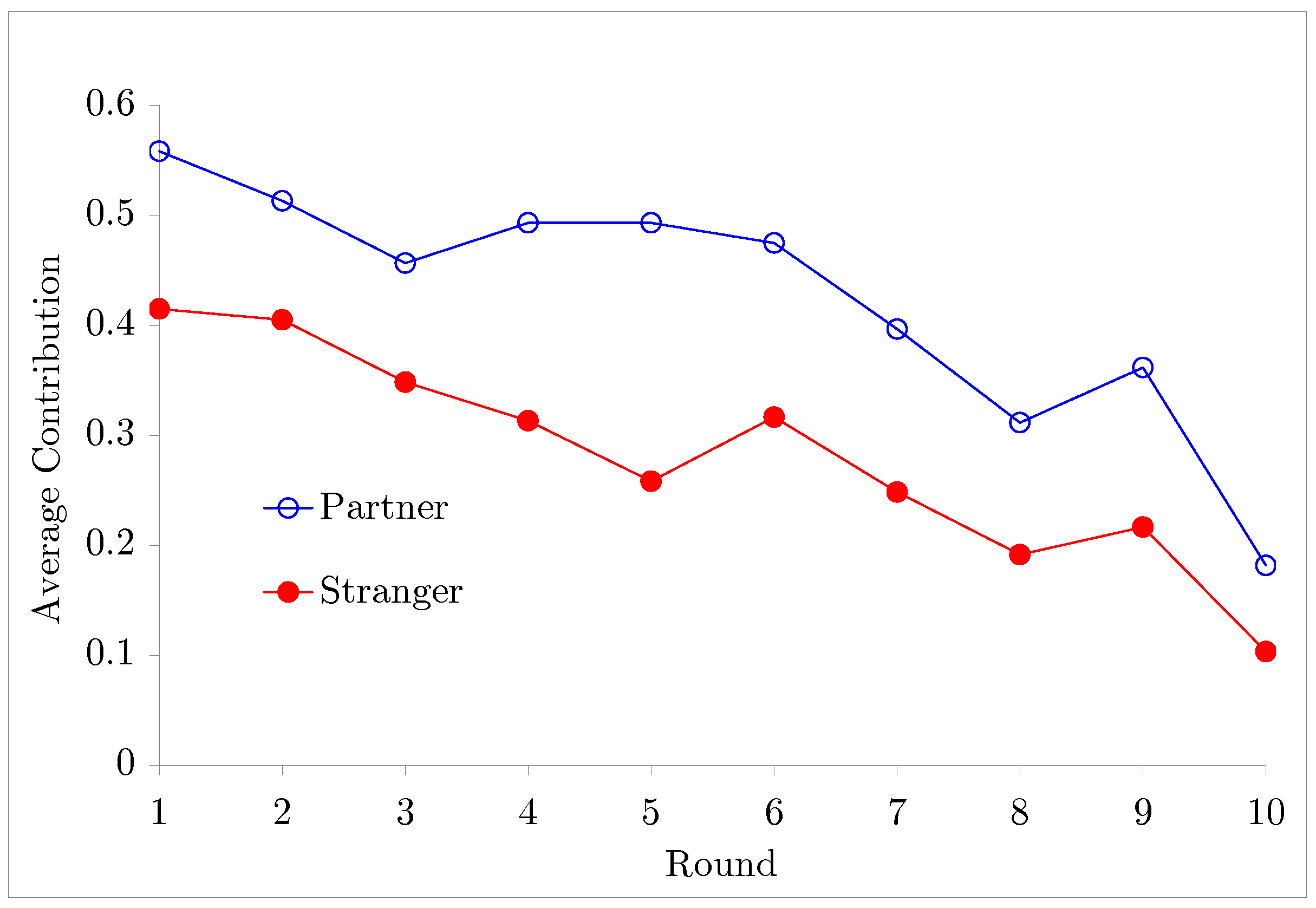
Since Andreoni (1988) found that the average contribution from Strangers group was relatively larger than that from Partners group, there are lots of papers investigating the difference between Strangers and Partners group, but the results are inconclusive. Andreoni and Croson (2008) summarize the results from many replications and studies that have explored this question: ‘Nonetheless, this summary of results does little to clear up the picture. In all, four studies find more cooperation among Strangers, five find more by Partners, and four fail to find any difference at all.’ The answer to whether partners group or strangers group contribute more is really mixed. We will re-examine the treatment effect of rematching in this paper. Among all the replications of Partners vs. Strangers Game, the experiments from Croson (1996) and Keser and Van Winden (2000) are identical except for the number of rounds. Interestingly, both papers found that the average contribution from Partners group was higher than that from Strangers group.

Table 1. Data description.

Authors	Croson3		Keser and Winden
	Strangers	Partners	Strangers	Partners
subjects no.	24	24	120	40
$MPCR$	$0.5$	$0.5$	$0.5$	$0.5$
G	4	4	4	4
T	10	10	25	25
e	25	25	10	10

describes the data and various features of the experiments, and Figure 1 shows the average contribution for each round in Croson (1996). Note that it seems to be straightforward to compare two samples in Figure 1 if all samples are independently distributed. In many experimental studies, however, this assumption is violated: usually, $y_{it}$ is cross-sectionally and serially correlated. Under this circumstance, a conventional z-score test with $y_{it}$ for each $t,$ or with time series averages of $y_{it}$ becomes invalid unless the cross sectional dependence is considered properly. For the same reason, other statistics used in practice become invalid as well.2

For each study, controlled and treated groups may be defined and then the treatment effects can be measured. For all cases, the null hypothesis of interest becomes no treatment effect or the same overall outcomes given by

$${\mathcal{H}}_0:\mathbb{E}{\pi }_c=\mathbb{E}{\pi }_{\tau },$$

(3)

where ${\pi }_c$ and ${\pi }_{\tau }$ are controlled and treated overall outcomes, respectively. Under the null hypothesis, the overall outcomes become the same regardless of the number of rounds.

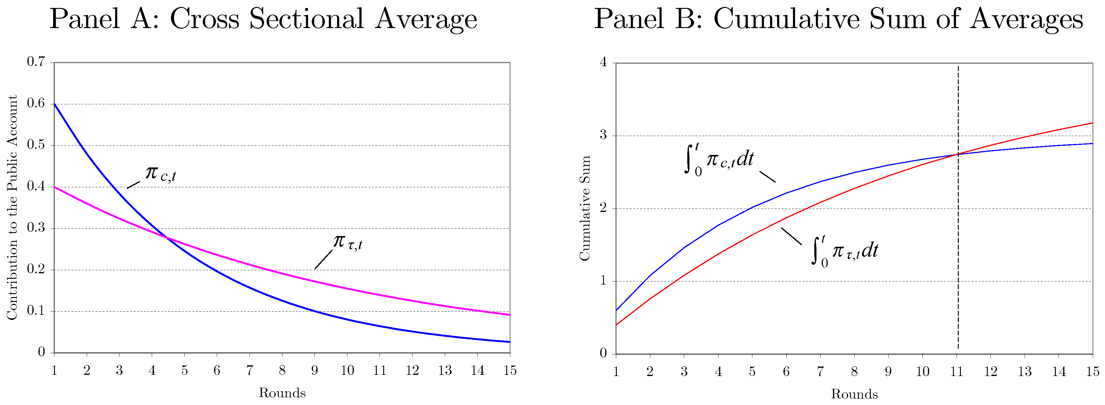
The overall outcomes can be measured by the area below of the cross sectional averages. Let ${\pi }_{s,t}$ be the true, but unknown decay function for the sth experiment. Then, the overall outcome can be defined as ${\pi }_s={\int }_0^{\infty }{\pi }_{s,t}dt.$4 When the treated experimental outcome at time t is always greater or equal to the controlled one for all $t,$ that is, ${\pi }_{\tau ,t}>{\pi }_{c,t},$ then the overall treatment effects, $\mathsf{\Pi }={\pi }_{\tau }-{\pi }_c,$ becomes positive. However, when ${\pi }_{ct}$ is crossing over ${\pi }_{\tau ,t}$, it is hard to judge whether or not the treatment effects become positive or negative. Figure 2 demonstrates such an artificial case where the null hypothesis is not easy to be tested.5 Panel A in Figure 2 shows the hypothetical average of the controlled and treated outcomes for each round. The decay rate for the controlled group is faster than that for the treated group, but the initial average outcome for the controlled group is higher than that for the treated group. The overall effects can be measured by the areas below the average of the outcomes which are displayed in Panel B in Figure 2. Evidently, the treatment effect is depending on the number of rounds. The treatment effect becomes negative, zero and positive when the final round T becomes $T<11,$ $T=11,$ and $T>11.$

3. Statistical Model

There is one important and distinctive feature of the repeated lab-experimental data: a nonstationary initial condition. This unique feature is rarely seen in conventional data, and, more importantly, the estimation without accounting for this feature is invalid, which consequently leads to wrong judgements. This section provides a new statistical model for this nonstationary initial condition.

3.1. Statistical Modelling Nonstationary Initial Condition

Here, we statistically approximate the decay rate in Figure 1 and Figure 2 as an exponential decay function. We do not aim to model or explain the unknown decay function theoretically but rather approximate it. In other words, we model it statistically. In repeated experiments, subjects are randomly selected but exhibit common behavior. Typically, responses decrease over successive rounds as shown in Figure 1. Interestingly, such common behavior, or highly cross-sectionally correlated behavior, can be generated if the true mean of the initial contributions is different from the mean of the contributions in the long run. Note that, in this subsection, we will ignore the subscript s for notational convenience.

Define $y_{N,t}$ to be the cross-sectional average of $y_{it}$ at time $t.$ When $t=1,$ we let

$$y_{N,1}=\mu +{ϵ}_{n,1}.$$

(4)

Meanwhile, $t>1,$ we assume that the cross-sectionally aggregated series follows AR(1) process:

$$y_{N,t}=a\left(1-\rho \right)+\rho y_{N,t-1}+{ϵ}_{N,t},\mathrm{for}t\ge 2,$$

(5)

where a can be treated as the long run value of $y_{N,t}$ in the sense that

$$\underset{t\to \infty }{\lim }\mathbb{E}{y}_{N,t}=a\left(1-\rho \right)+\rho \underset{t\to \infty }{\lim }\mathbb{E}{y}_{N,t-1},$$

(6)

so that

$$\underset{t\to \infty }{\lim }\mathbb{E}{y}_{N,t}=a,$$

(7)

since ${\lim }_{t\to \infty }\mathbb{E}{y}_{N,t-1}={\lim }_{t\to \infty }\mathbb{E}{y}_{N,t}.$ Usually, the expected value of initial outcome is not the same as the long run outcome. That is, $\mu \ne a.$ Statistically, the transitory behavior of $y_{Nt}$ due to the nonstationary initial condition in (4) can be modeled by

$$y_{N,t}=a+\left(\mu -a\right){\rho }^{t-1}+e_{N,t},\mathrm{for}t=1,\dots ,T,$$

(8)

where the error follows an AR(1) process with the nonstationary initial condition.

$$e_{N,t}=\rho e_{N,t-1}+{ϵ}_{N,t}\mathrm{with}{e}_{N,1}={ϵ}_{N,1}.$$

If the initial mean, $\mu ,$ is different from the long run mean, $a,$ then $y_{Nt}$ have a time decay function ${\rho }^{t-1}$ as it is shown in (8).

One of the most interesting features of the repeated games is the convergent behavior. As t approaches the last round, the fraction of free riders increases and, for some games, this fraction becomes one.6 That is, the average outcome, $y_{N,t},$ is converging to the long run equilibrium. This implies that the variance of the random error should be decreasing over time as well. Otherwise, the fraction of free riders does not converge to unity as t increases. To reflect this fact, we assume that the variance of $e_{N,t}$ is shrinking at the rate ${\rho }^{t-1}$ over time.7

$$e_{N,t}=u_{N,t}{\rho }^{t-1}\mathrm{for}0\le \rho \le 1.$$

(9)

This implies that at $t=1,$ ${ϵ}_{N,1}=u_{N,1}.$ Since $y_{N,t}$ is bounded between zero and one, the initial error term, $u_{N,1},$ should be bounded between $-\mu$ and $1-\mu .$ We assume that this restricted condition holds with $t>1$ as well. That is, $u_{N,t}$ is independently distributed but bounded between $-\mu$ and $1-\mu .$ Statistically, we write as

$$u_{N,t}\sim idB{\left(0,{\sigma }^2\right)}_{-\mu }^{1-\mu },$$

(10)

where $id$ stands for ‘independently distributed’, B implies boundedness, and the superscript and subscript show the upper and lower bounds.

3.2. Features of New Statistical Model

In the previous subsection, we assume that the nonstationary initial condition model can approximate well the cross-sectional average of individual outcomes. In this subsection, we consider the possibility that the aggregated model in (8) through (10) holds for all subjects. That is, we further assume that the stochastic process for $y_{it}$ can be written as

$$y_{it}=a_i+\left({\mu }_i-a_i\right){\rho }^{t-1}+e_{it}\mathrm{for}{e}_{it}=u_{it}{\rho }^{t-1},\mathrm{and}{u}_{it}\sim idB{\left(0,{\sigma }_i^2\right)}_{-{\mu }_i}^{1-{\mu }_i},$$

(11)

where the experimental outcome $y_{it}$ is normalized by the maximum number of tokens so that $0\le y_{it}\le 1$ always for all i and $t.$ The long run value of $y_{it}$ is $a_i,$ ${\mu }_i$ is the unknown initial mean of $y_{i1},$ $\rho$ is the decay rate and $e_{it}$ is the approximation error. Note that $u_{it}$ is a bounded, but independent random variable with mean zero and variance ${\tilde{\sigma }}_i^2,$ or $u_{it}\sim iB{\left(0,{\tilde{\sigma }}_i^2\right)}_{-{\mu }_i}^{1-{\mu }_i}.$ As t increases, the unconditional mean of individual outcome, $y_{it},$ converges $a_i$ which can be interpreted as a long run steady state.

If the assumption in (11) holds, then the simple stochastic process for $y_{it}$ may explain the temporal cross-sectional dependence. When $t=1$ (initial round), the individual outcome, $y_{i1},$ is not cross sectionally dependent since subjects are randomly selected. However, when $t\ge 2,$ the individual outcome becomes cross-sectionally dependent due to the time varying mean part, $\left({\mu }_i-a_i\right){\rho }^{t-1}.$ The common factor model captures the kind of behavior described in Ashley et al. (2010): the previous group outcome affects the experimental outcome for each subject. To see this, consider the fact that the group means excluding the ith subject outcome, ${\left(G-1\right)}^{-1}{\sum }_{j\ne i}^G{y}_{it},$ is similar to the group mean of $G^{-1}{\sum }_{i=1}^G{y}_{it}.$ In addition, the group mean is similar to the cross sectional average: $G^{-1}{\sum }_{i=1}^G{y}_{it}\simeq N^{-1}{\sum }_{i=1}^N{y}_{it}={\mu }_N{\rho }^{t-1}+e_{N,t}$ where ${\mu }_N$ and $e_{N,t}$ are the cross-sectional averages of ${\mu }_i$ and $e_{it}.$ Note that with large N, $e_{N,t}$ is close to zero, so that this term can be ignored. Statistically $e_{N,t}=O_p\left(N^{-1/2}\right)$ for any $t.$ Hence, the subject’s outcome at time t can be rewritten as

$$y_{it}=\frac{{\mu }_i}{{\mu }_N}\rho \times \left({\mu }_N{\rho }^{t-2}\right)+e_{it}+O_p\left(N^{-1/2}\right).$$

The first term represents the marginal rate of the relative contribution of each subject, and the second term is the group average in the previous round, and the last two terms are random errors.

Nonetheless, we do not attempt to model the implicit behaviors of individuals, such as selfish, reciprocal and altruistic behaviors. Instead, we model the time varying patterns of the outcome (contribution to group account) statistically. By following Ambrus and Greiner (2012), we approximate heterogeneous behaviors of subjects econometrically into three groups: increasing, decreasing and fluctuating. The increasing group includes two subgroups of subjects: subjects contribute all tokens to the public account for all rounds or contribute more tokens over successive rounds. Similarly, the decreasing group includes the two subgroups of subjects: Subjects do not contribute at all, or subjects contribute fewer tokens over rounds. Lastly, a fluctuating or confused subject is neither in the decreasing or increasing group.

In public goods games, if the long run Nash equilibrium occurs (or if $a_i=0$ and $0<\rho <1$), the fraction of free riders increases over rounds. Meanwhile, if $a_i=1$ and $0<\rho <1,$ then the unconditional mean of the individual outcome, $y_{it},$ converges to the Pareto optimum $\left(a_i=1\right)$. Furthermore, except for the initial round, the experimental outcomes are cross-sectionally dependent so that individual’s decision depends on the overall group outcome. Lastly, if the decay rate becomes unity or $\rho =1$, then the individual outcome becomes purely random.

To be specific, we can consider the following three dynamic patterns:

$$y_{it}=\left\{\begin{array}{cc}{\mu }_i{\rho }^{t-1}+e_{1,it}\hfill & \mathrm{if}i\in G_1,\mathrm{or}{a}_i=0\mathrm{and}0<\rho <1,\hfill \\ {\mu }_i+e_{2,it}\hfill & \mathrm{if}i\in G_2,\mathrm{or}\rho =1,\hfill \\ 1-\left(1-{\mu }_i\right){\rho }^{t-1}+e_{3,it}\hfill & \mathrm{if}i\in G_3,\mathrm{or}{a}_i=1\mathrm{and}0<\rho <1.\hfill \end{array}\right.$$

(12)

For groups $G_1$ and $G_3$, the contribution is decaying each round at the same rate, $\rho .$ If a subject belongs to $G_1$, the contribution is decreasing over rounds and, if she belongs to $G_3$, the contribution is increasing. The remaining subjects are classified together in a ‘fluctuating’ group. For non-fluctuating groups ($G_1$ and $G_3$), the random errors can be rewritten as $e_{s,it}=u_{s,it}{\rho }^{t-1}$ for $s=1,3.$ Hence, as round increases, the variance of $e_{s,it}$ decreases and eventually converges to zero. Meanwhile, the random error for $G_2$ is not time varying since $\rho$ is always unity.

Let $N_1$ be the number of subjects in $G_1$ and $n_1=N_1/N.$ Similarly, we can define $N_2$ and $N_3$as the numbers of subjects in $G_2$ and $G_3,$ and $n_2$ and $n_3$as their fractions, respectively. The sample cross-sectional averages for each round under homogeneity (only $G_1$ exists) and heterogeneity can be written as

$$\frac{1}{N}{\sum }_{i=1}^N{y}_{it}=\left\{\begin{array}{cc}\mu {\rho }^{t-1}+e_{Nt}^{†}\hfill & \mathrm{if}\mathrm{all}i\in G_1,\hfill \\ \tau +\phi {\rho }^{t-1}+e_{Nt}^{\ast }\hfill & \mathrm{if}\mathrm{some}i\notin G_1,\hfill \end{array}\right.$$

(13)

where $\tau =n_2\mu +n_3$, $\phi =\mu -\tau ,$ and

$$\begin{array}{ccc}\hfill e_{Nt}^{†}& =& N^{-1}{\sum }_{i=1}^N{e}_{it}+{\rho }^{t-1}{N}^{-1}{\sum }_{i=1}^N\left({\mu }_i-\mu \right),\hfill \\ \hfill e_{Nt}^{\ast }& =& {\rho }^{t-1}{N}^{-1}{\sum }_{i=1}^N\left({\mu }_i-\mu \right)+\left(1-{\rho }^{t-1}\right)N^{-1}{\sum }_{i=1}^{N_2}\left({\mu }_i-\mu \right)+N^{-1}{\sum }_{i=1}^N{e}_{it}.\hfill \end{array}$$

Therefore, the time varying behavior of the cross-sectional averages under homogeneity become very different from those under heterogeneity. First, under homogeneity, the average outcome decreases each round and converges to zero. However under heterogeneity, depending on the value of $\phi ,$ the average outcome may decrease $\left(\phi >0\right)$, increase $\left(\phi <0\right)$ or does not change at all $\left(\phi =0\right)$ over rounds. Second, the variance of the random part of the cross-sectional average, $e_{Nt}^{†},$ under homogeneity is much smaller than that under heterogeneity. In other words, the cross-sectional averages under heterogeneity become much more volatile than those under homogeneity. Third, both random errors, $e_{Nt}^{†}$ and $e_{Nt}^{\ast },$ are serially correlated. However, the serial correlation of the random errors under homogeneity, $E{e}_{Nt}^{†}{e}_{Nt-s}^{†},$ goes away quickly as s increases, meanwhile the serial correlation under heterogeneity, $E{e}_{Nt}^{\ast }{e}_{Nt-s}^{\ast }$ never goes to zero even when $s\to \infty$ as long as $n_2\ne 0.$

It is not hard to show that under heterogeneity the cross-sectional variance of $y_{it}$ diverges over rounds. In this case, the estimation of the treatment effects is not straightforward since $\tau$ and $\phi$ in (13) cannot be identified in some cases.8 We leave the case of heterogeneity for future work, and mainly focus on the estimation of the treatment effects under homogeneity. The homogeneity assumption is testable. One may test the convergence directly by using Phillips and Sul (2007) or Kong et al. (2018). Particularly the weak $\sigma$—convergence test proposed by Kong et al. (2018) is more suitable for the convergence test since the relative convergence test by Phillips and Sul (2007) requires somewhat more restrictive conditions than the weak $\sigma -$convergence test by Kong et al. (2018).

The contributions to the public account up to the last round T can be measured by the following statistic.

$${\sum }_{t=1}^T\frac{1}{N}{\sum }_{i=1}^N{y}_{it}={\mu }_N\frac{1-{\rho }^T}{1-\rho }+e_{N,T},$$

where

$$e_{N,T}={\sum }_{t=1}^T\frac{1}{N}{\sum }_{i=1}^N{e}_{it}={\sum }_{t=1}^T\frac{1}{N}{\sum }_{i=1}^N{u}_{it}{\rho }^{t-1}=O_p\left(N^{-1/2}\right),$$

since the sum of ${\rho }^{2t-2}$ over T is $O\left(1\right).$9 The estimation of the overall treatment can be done simply by comparing the two means, provided the subjects in the two experiments are independently and randomly selected. Let $N=\min \left[N_c,N_{\tau }\right],$ where $N_c$ and $N_{\tau }$ are the total numbers of subjects for the controlled and treated experiments, respectively. Then, from (11), the probability limit of the average difference becomes the treatments effect (TE) given by

$$\begin{array}{ccc}\hfill TE& =& {\mathrm{plim}}_{N\to \infty }\left[{\sum }_{t=1}^T\frac{1}{N_c}{\sum }_{i=1}^{N_c}{y}_{c,it}-{\sum }_{t=1}^T\frac{1}{N_{\tau }}{\sum }_{i=1}^{N_{\tau }}{y}_{\tau ,it}\right]\hfill \\ & =& {\mu }_c\frac{1-{\rho }_c^T}{1-{\rho }_c}-{\mu }_{\tau }\frac{1-{\rho }_{\tau }^T}{1-{\rho }_{\tau }},\hfill \end{array}$$

(14)

where ${\mu }_c$ and ${\mu }_{\tau }$ are the cross-sectional mean of the initial contributions. When ${\mu }_c={\mu }_{\tau },$ the overall treatment effect with the slower decay rate is higher than the treatment effect with the faster decay rate. When two experimental outcomes cross over each other, the overall effect becomes ambiguous. Mathematically, this case can be written as ${\mu }_c>{\mu }_{\tau }$ but ${\rho }_c<{\rho }_{\tau }$. Suppose that, with a fixed T (say $T=10),$ the overall effect in the crossing-over case is identical between the two experiments. Then, such a result does not become robust since, with more repetitions, the experimental outcome with the slower decay rate must be higher than that with the faster decay rate. Hence, for a such case, the following asymptotic treatment effect can measure the two outcomes robustly and effectively:

$$\mathrm{Asy}.\mathrm{TE}=\mathsf{\Pi }=\underset{T\to \infty }{\lim }TE=\frac{{\mu }_c}{1-{\rho }_c}-\frac{{\mu }_{\tau }}{1-{\rho }_{\tau }}={\pi }_c-{\pi }_{\tau },\mathrm{let}’\mathrm{s}\mathrm{say}.$$

(15)

3.3. Estimation of Overall Treatment Effects

The experimental outcomes will converge to zero when the dominant strategy is Nash bargaining.10 It is better to use this convergence result in the estimation of the asymptotic treatment effect. That is, the percentage of free-riding is assumed to become one as the total number of rounds increases.11 If there are multiple dominant strategies in a game, then the experimental outcomes do not need to converge to a certain value. In this case, the outcome for each round may be volatile and, more importantly, the cross-sectional variance will increase over rounds.

The estimation of the asymptotic treatment effects requires the estimation of two unknown parameters; $\mu$ and $\rho .$ There are two ways to estimate both parameters jointly: nonlinear least squares estimators (NLS) and log transformed least squares estimation with the cross-sectionally averaged data. Below, we first discuss the potential problems associated with NLS estimation, and then go on to show the simple log trend regression.

Nonlinear Least Squares (NLS) Estimation

To estimate $\mu ,$ one may consider estimating ${\mu }_i$ first by running the following NLS regression for each i:

$$y_{it}=f\left({\mu }_i,\rho \right)+e_{it}={\mu }_i{\rho }^{t-1}+e_{it},\mathrm{let}\text{’}\mathrm{s}\mathrm{say}.$$

It is well known that the NLS estimators for ${\mu }_i$ and $\rho$ are inconsistent as $T\to \infty$ because ${\sum }_{t=1}^{\infty }{\left(f\left({\mu }_i,\rho \right)-m_t\left({\mu }_i^{+},{\rho }^{+}\right)\right)}^2=M<\infty$ for ${\mu }_i\ne {\mu }_i^{+}$ and $\rho \ne {\rho }^{+}.$ See Malinvaud (1970) and Wu (1981) for more detailed discussions. However, there is a way to estimate $\mu$ and $\rho$ by using cross sectional averages. Consider the following regression with cross-sectional averages

$$y_{N,t}={\mu }_N{\rho }^{t-1}+e_{N,t}.$$

(16)

For a given $T,$ as $N\to \infty ,$ ${\sum }_{i=1}^N{\sum }_{t=1}^T{\left({\mu }_i{\rho }^{t-1}-{\mu }_i^{+}{\left[{\rho }^{+}\right]}^{t-1}\right)}^2\to \infty$ for ${\mu }_i\ne {\mu }_i^{+}$ and $\rho \ne {\rho }^{+}.$ Therefore, both ${\mu }_N$ and $\rho$ can be estimated consistently as $N\to \infty .$ Denote the resulting estimators as ${\widehat{\mu }}_{\mathrm{nls}}$ and ${\widehat{\rho }}_{\mathrm{nls}}.$ We will discuss the underlying asymptotic theory in the next section, but, in the meantime, we want to emphasize here that the fastest convergence rate for ${\widehat{\rho }}_{\mathrm{nls}}$ is $\sqrt{N}$ even when $T,N\to \infty$ jointly.

Logarithm Transformation

Alternatively, the nonlinear regression in (16) can be transformed into a linear regression by taking the logarithm in $y_{N,t}$.12 Observe this:

$$\log y_{N,t}=\log {\mu }_N+\left(\log \rho \right)\left(t-1\right)+\log \left(1+\frac{e_{N,t}}{{\mu }_N{\rho }^{t-1}}\right).$$

(17)

From (9), the last term can be rewritten as

$$\log \left(1+\frac{e_{N,t}}{{\mu }_N{\rho }^{t-1}}\right)=\log \left(1+\frac{u_{N,t}}{{\mu }_N}\right)=\frac{u_{N,t}}{{\mu }_N}+O_p\left(N^{-1}\right)=v_{N,t}^{\ast }+O_p\left(N^{-1}\right),$$

(18)

where $u_{N,t}=N^{-1}{\sum }_{i=1}^N{u}_{it}.$ Hence, the following simple trend regression can be used to estimate $\log {\mu }_N$ and $\log \rho$:

$$\log \left(\frac{1}{N}{\sum }_{i=1}^N{y}_{it}\right)=\log {\mu }_N+\left(\log \rho \right)\left(t-1\right)+v_{N,t};t=1,...,T.$$

(19)

Taking the exponential function of $\widehat{\log {\mu }_N}$ and $\widehat{\log \rho }$ provides consistent estimators for ${\widehat{\mu }}_N$ and $\widehat{\rho }$, respectively. The asymptotic properties of the trend regression in (19) will be discussed in detail shortly, but here note that the convergence rate for $\widehat{\rho }$ is much faster than ${\widehat{\rho }}_{\mathrm{nls}}.$ However, this does not always imply that $\widehat{\rho }$ is more accurate than ${\widehat{\rho }}_{\mathrm{nls}}$, especially with small $N.$ It is possible that the minimum value of the cross-sectional averages of $y_{it}$ can be near-zero or zero. In this case, the dependent variable in (19) is not well-defined.

4. Asymptotic Theory

This section provides the asymptotic theory for the proposed estimators in (16) and (19). We make the following assumptions.

Assumption A: Bounded Distributions

(A.1) 

${\mu }_i$is independent and identically distributed with mean$\mu$and variance${\sigma }_{\mu }^2$, but it is bounded between 0 and 1:${\mu }_i\sim iidB{\left(\mu ,{\sigma }_{\mu }^2\right)}_0^1$

(A.2) 

$e_{it}=u_{it}{\rho }^{t-1}$for$0\le \rho \le 1$where$u_{it}$is independently distributed with mean zero and variance${\sigma }_i^2$, but it is bounded between$-{\mu }_i$and$1-{\mu }_i.$That is,$u_{it}\sim idB{\left(0,{\sigma }_i^2\right)}_{-{\mu }_i}^{1-{\mu }_i}.$

Assumption B: Data Generating Process

The data generating process is given by$y_{it}={\mu }_i{\rho }^{t-1}+e_{it}.$

Under Assumptions A and B, it is easy to show that, if $0\le \rho <1,$ all subjects’ outcomes become zero in the long run:

$$\underset{t\to T^{\ast }}{\lim }{y}_{it}=0\mathrm{for}\mathrm{all}i.$$

In other words, $y_{it}$ converges to zero. Assumption A.2 implies no serial dependence in $u_{it}$ for the sake of simplicity. We will show later that we cannot find any empirical evidence suggesting that $u_{it}$ is serially correlated. In addition, see Remark 5 and 6 for more discussion of the ramifications of the violation of Assumption A.2.

Define the nonlinear least squares estimator in (16) as the minimizer of the following loss function:

$$\arg \underset{{\mu }_N,\rho }{\min }{\sum }_{t=1}^T{\left(y_{N,t}-{\mu }_N{\rho }^{t-1}\right)}^2.$$

Meanwhile, the ordinary least squares estimator in (19) is defined as

$$\left[\begin{array}{c}{\widehat{\log \mu }}_N\\ \widehat{\log \rho }\end{array}\right]={\left[\begin{array}{cc}\sum _{t=1}^{T}1& \sum _{t=0}^{T-1}t\\ \sum _{t=0}^{T-1}t& \sum _{t=0}^{T-1}{t}^2\end{array}\right]}^{-1}\left[\begin{array}{c}\sum _{t=1}^T\log y_{N,t}\\ \sum _{t=1}^T\left(t-1\right)\log y_{N,t}\end{array}\right].$$

(20)

Since the point estimates are obtained by running either nonlinear or linear time series regression, the initial mean, ${\mu }_i,$ for each subject is not directly estimated, but the cross-sectional mean, ${\mu }_N,$ is estimated. Define ${\tilde{\mu }}_N$ as an estimator for ${\mu }_N.$ Then, the deviation from its true mean $\mu$ can be decomposed as

$${\tilde{\mu }}_N-\mu =\left({\tilde{\mu }}_N-{\mu }_N\right)+\left({\mu }_N-\mu \right).$$

(21)

Since ${\mu }_N-\mu =O_p\left(N^{-1/2}\right),$ ${\tilde{\mu }}_N-\mu$ also becomes $O_p\left(N^{-1/2}\right)$ as long as ${\tilde{\mu }}_N-{\mu }_N=O_p\left(N^{-1/2}{T}^{-\kappa }\right)$ for $\kappa >0.$ There are two ways to derive the limiting distribution for ${\tilde{\mu }}_N$, depending on the definition of the regression errors or the definition of the regression coefficients. First, the error terms can be defined as in (16) and (19). Then, the limiting distribution of ${\tilde{\mu }}_N-{\mu }_N$ can be derived, which is the first term in (21). After that, the limiting distribution of ${\tilde{\mu }}_N-\mu$ can be obtained by adding the limiting distribution of ${\mu }_N-\mu$ to that of ${\tilde{\mu }}_N-{\mu }_N.$

Second, the error terms or the coefficient terms may be re-defined as follows:

$$\begin{array}{ccc}\hfill y_{N,t}& =& \mu {\rho }^{t-1}+{\epsilon }_{N,t},\mathrm{for}{\epsilon }_{N,t}=\left[u_{N,t}+\left({\mu }_N-\mu \right)\right]{\rho }^{t-1},\hfill \end{array}$$

(22)

$$\begin{array}{ccc}\hfill \log y_{N,t}& =& \log \mu +\left(\log \rho \right)\left(t-1\right)+v_{N,t}\mathrm{for}{v}_{N,t}=\left[v_{N,t}^{\ast }+\left({\mu }_N-\mu \right)\right]/\mu .\hfill \end{array}$$

(23)

Of course, the limiting distributions of the estimators in (16) and (19) are identical to those in (22) and (23). Nonetheless, it is important to address how to estimate the variance of ${\mu }_i$ consistently. We will discuss this later but now provide the limiting distributions for the estimators of $\mu$ and $\rho$ in (22) and (23) here first. Let $\widehat{\mu }=\exp ({\widehat{\log \mu }}_N)$ and $\widehat{\rho }=\exp (\widehat{\log \rho }),$ where ${\widehat{\log \mu }}_N$ and $\widehat{\log \rho }$ are LS estimators of the coefficients given in (23).

Theorem 1.

Limiting Distributions

Under Assumption A and B, as $N,T\to \infty$ jointly,

(i) the limiting distributions of the NLS estimators in (22) are given by

$$\left[\begin{array}{c}\sqrt{N}\left({\widehat{\mu }}_{nls}-\mu \right)\\ \sqrt{N}\left({\widehat{\rho }}_{nls}-\rho \right)\end{array}\right]{\to }^d\mathcal{N}\left(\left[\begin{array}{c}0\\ 0\end{array}\right],\left[\begin{array}{cc}{\mathsf{\Omega }}_{11}& {\mathsf{\Omega }}_{12}\\ {\mathsf{\Omega }}_{12}& {\mathsf{\Omega }}_{22}\end{array}\right]\right),$$

(24)

where

$$\begin{array}{ccc}\hfill {\mathsf{\Omega }}_{11}& =& \frac{3{\rho }^2+{\rho }^4-5{\rho }^6+1}{{\left(1+{\rho }^2\right)}^3}{\sigma }^2+\left[\left(1+2{\rho }^2\right)-\left(2-\rho \right){\rho }^3\left(1+{\rho }^2\right)\right]{\sigma }_{\mu }^2,\hfill \\ \hfill {\mathsf{\Omega }}_{12}& =& -\rho {\left(1-{\rho }^2\right)}^2\left(1+3{\rho }^2\right)\frac{{\sigma }^2}{\mu {\left(1+{\rho }^2\right)}^3}-\left(1+{\rho }^2-{\rho }^3\right)\left(1-\rho \right)\frac{1-{\rho }^2}{\mu }{\sigma }_{\mu }^2\rho ,\hfill \\ \hfill {\mathsf{\Omega }}_{22}& =& \frac{2{\left(1-{\rho }^2\right)}^3{\rho }^2}{{\mu }^2{\left(1+{\rho }^2\right)}^3}{\sigma }^2+{\left(1-\rho \right)}^2{\left(1-{\rho }^2\right)}^2\frac{{\rho }^2{\sigma }_{\mu }^2}{{\mu }^2}.\hfill \end{array}$$

(ii) The limiting distributions of the LS estimators in (23) are given by

$$\left[\begin{array}{c}\sqrt{N}\left(\widehat{\mu }-\mu \right)\\ \sqrt{N}{T}^{3/2}\left(\widehat{\rho }-\rho \right)\end{array}\right]{\to }^d\mathcal{N}\left(\left[\begin{array}{c}0\\ 0\end{array}\right],\Sigma \right)where\Sigma =\left[\begin{array}{cc}{\sigma }_{\mu }^2& 0\\ 0& 12{\rho }^2{\sigma }^2/{\mu }^2\end{array}\right].$$

(25)

See Appendix A for the detailed proof of Theorem 1. Here, we provide an intuitive explanation of the results, especially regarding the convergence rate. The convergence rate of the NLS estimators is $\sqrt{N}$ even under the condition of $N,T\to \infty$ jointly. The underlying reason is as follows. The first derivative of $\mu {\rho }^{t-1}$ with respect to $\rho ,$ $f_{\rho ,t},$ is $\mu \left(t-1\right){\rho }^{t-2},$ so that ${\sum }_{t=1}^T{f}_{\rho ,t}^2=O\left(1\right)$ since ${\lim }_{t\to \infty }t{\rho }^t=0.$ However, the order in probability of the regression errors is $O_p\left(N^{-1/2}\right)$, which determines the convergence rate of ${\widehat{\rho }}_{\mathrm{nls}}.$ Meanwhile, the LS estimators with the logged cross-sectional averages in (23) are free from this problem. That is why the convergence rate of the estimator for $\log \rho$ is $\sqrt{N}{T}^{3/2}.$ From the delta method, $\widehat{\rho }-\rho =\rho (\widehat{\log \rho }-\log \rho )+O_p\left(N^{-1}{T}^{-3}\right).$ Hence, the convergence rate of $\widehat{\rho }-\rho$ is also $\sqrt{N}{T}^{3/2}.$ As we discussed under (21), the convergence rate of $\widehat{\mu }$ is totally dependent on that of ${\mu }_N-\mu ,$ which is $\sqrt{N}.$ We will show later by means of Monte Carlo simulation that the LS estimators have better finite sample performance than NLS estimators.

Here are some important remarks regarding the properties of the considered estimators.

Remark 1.

Limiting Distributions for Fixed T

Define ${\widehat{\theta }}_{nls}={\left({\widehat{\mu }}_{nls}{\widehat{\rho }}_{nls}\right)}^{\prime },$ $\widehat{\theta }={\left(\widehat{\mu }\widehat{\rho }\right)}^{\prime }$ and $\theta ={\left(\mu \rho \right)}^{\prime }.$ Under Assumption A and B, as $N\to \infty$ with fixed $T,$ the limiting distributions are given by

$$\sqrt{N}\left({\widehat{\theta }}_{nls}-\theta \right){\to }^d\mathcal{N}\left(0,{\mathsf{\Omega }}_T\right),\sqrt{N}\left(\widehat{\theta }-\theta \right){\to }^d\mathcal{N}\left(0,{\Sigma }_T\right).$$

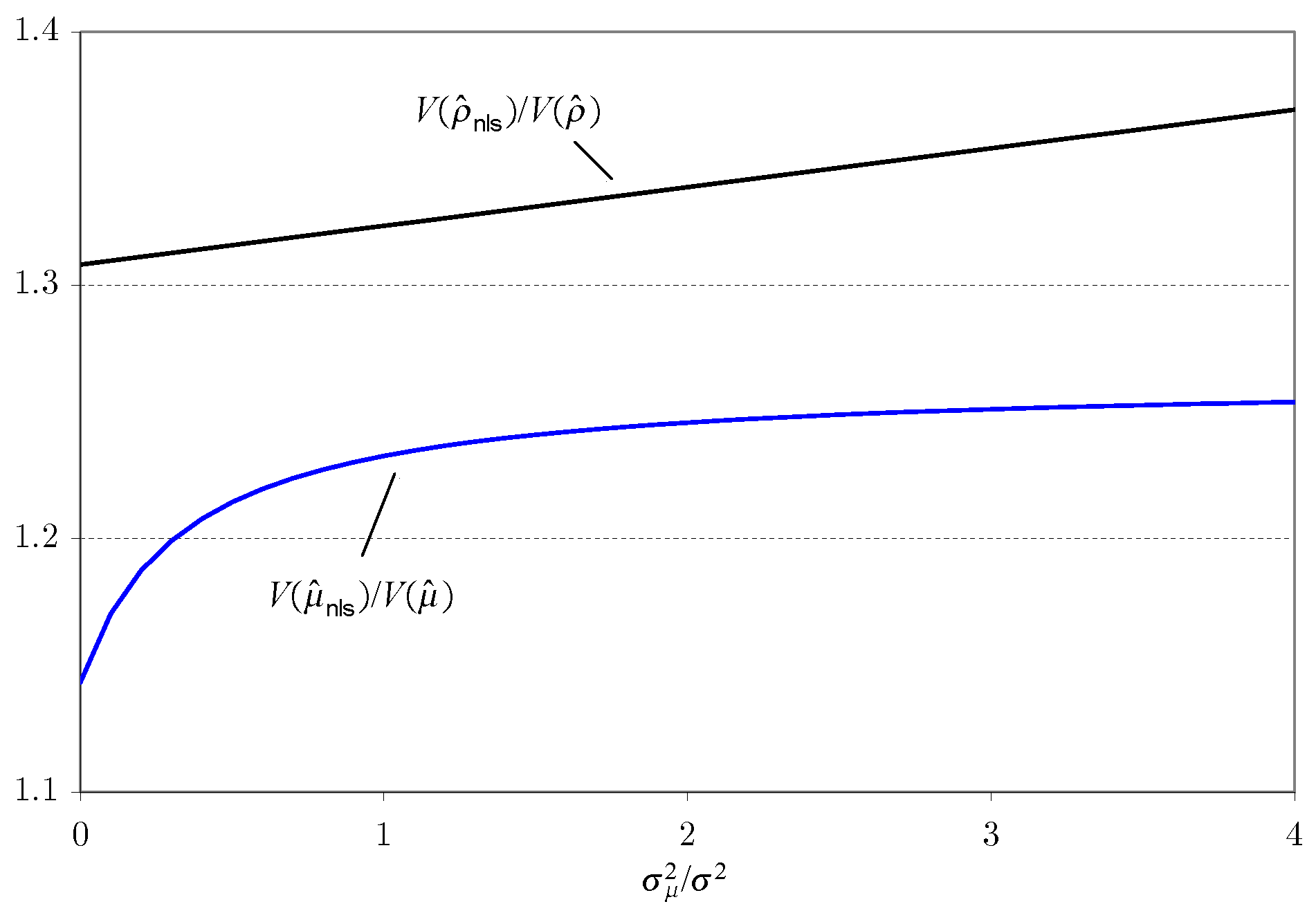
The variances ${\mathsf{\Omega }}_T$ and ${\Sigma }_T$ are finite constants but are not expressed explicitly since their formulae are very complicated. To evaluate and compare the two variances analytically, we set $T=10$ and $\rho =0.9$.13 With these values, the relative variance, ${\mathsf{\Omega }}_T/{\Sigma }_T,$ becomes a function of the relative variance of ${\sigma }_{\mu }^2/{\sigma }^2.$ Figure 3 displays the relative variance of ${\mathsf{\Omega }}_T/{\Sigma }_T$ to ${\sigma }_{\mu }^2/{\sigma }^2.$ Obviously, the LS estimators are more efficient than the NLS estimators because the variance of the LS estimator is always smaller than that of the NLS estimator for all ${\sigma }_{\mu }^2/{\sigma }^2\ge 0$. Interestingly, as ${\sigma }_{\mu }^2/{\sigma }^2$ increases, ${\mathsf{\Omega }}_T/{\Sigma }_T$ also increases.

Remark 2.

Consistent Estimator of ${\sigma }_{\mu }^2$

There are several ways to construct consistent estimators for ${\sigma }_{\mu }^2$ by utilizing the LS estimator $\widehat{\rho }.$ To save space, we do not report all consistent estimators. By means of (unreported) Monte Carlo simulation, we find that the following estimator for ${\sigma }_{\mu }^2$ provides the smallest variance among several estimators. The individual fixed effects, ${\mu }_i,$ can be estimated by running $y_{it}$ on ${\widehat{\rho }}^{t-1}.$ Note that, for any $t,$

$${\widehat{\rho }}^{t-1}={\rho }^{t-1}+\left(t-1\right){\rho }^{t-2}\left(\widehat{\rho }-\rho \right)+O_p\left(N^{-1}{T}^{-3}\right),$$

so that $y_{it}$ can be rewritten as

$$y_{it}={\mu }_i{\widehat{\rho }}^{t-1}+e_{it}^{+}for{e}_{it}^{+}=e_{it}+\left(t-1\right){\rho }^{t-2}\left(\widehat{\rho }-\rho \right){\mu }_i+O_p\left(N^{-1}{T}^{-3}\right).$$

(26)

Rewrite the LS estimator of ${\widehat{\mu }}_i$ in (26) as

$${\widehat{\mu }}_i={\mu }_i+{\left({\sum }_{t=1}^T{\widehat{\rho }}^{2t-2}\right)}^{-1}{\sum }_{t=1}^T{\widehat{\rho }}^{t-1}{e}_{it}^{+}.$$

By direct calculation, it is easy to show that this estimator is almost unbiased. Specifically,

$$\mathbb{E}\left({\sum }_{t=1}^T{\widehat{\rho }}^{t-1}{e}_{it}^{+}\right)=\frac{{\mu }_i^2}{{\mu }^2}\frac{12{\rho }^2\left({\rho }^2+{\rho }^4\right)}{{\left(1-{\rho }^2\right)}^{3}N{T}^3}{\sigma }^2.$$

Note that the convergence rate of ${\widehat{\mu }}_i$ over T is not $\sqrt{T}$ but $O\left(1\right)$ since the denominator term, ${\sum }_{t=1}^T{\widehat{\rho }}^{2t-2},$ becomes $O_p\left(1\right).$ However, the sample variance of ${\widehat{\mu }}_i$ estimates ${\sigma }_{\mu }^2$ consistently. As $N\to \infty ,$ the probability limit of the sample mean of ${\widehat{\mu }}_i$ becomes

$${plim}_{N\to \infty }\frac{1}{N}{\sum }_{i=1}^N{\widehat{\mu }}_i=\mu +{\left(\frac{1-{\rho }^{2T}}{1-{\rho }^2}\right)}^{-1}{plim}_{N\to \infty }\frac{1}{N}{\sum }_{i=1}^N{\sum }_{t=1}^T{\widehat{\rho }}^{t-1}{e}_{it}^{+}=\mu .$$

In addition, the probability limit of its variance is given by

$${plim}_{N\to \infty }\frac{1}{N}{\sum }_{i=1}^N{\left({\widehat{\mu }}_i-\frac{1}{N}{\sum }_{i=1}^N{\widehat{\mu }}_i\right)}^2={\sigma }_{\mu }^2.$$

Remark 3.

Limiting Distribution of Asymptotic Treatment Effects

Let the overall average individual outcome be

$$\widehat{\pi }=\frac{\widehat{\mu }}{1-\widehat{\rho }}.$$

To derive its limiting distribution, define $R=\left[\begin{array}{cc}{\left(1-\rho \right)}^{-1},& -\mu {\left(1-\rho \right)}^{-2}\end{array}\right]$. Then, by using the delta method, the limiting distribution of $\widehat{\pi }$ can be obtained from (25) directly:

$$\sqrt{N}\left(\widehat{\pi }-\pi \right){\to }^d\mathcal{N}\left(0,{\mathsf{\Omega }}_{\pi }\right),$$

(27)

where ${\mathsf{\Omega }}_{\pi }=R\Sigma R^{\prime }$ and Σ is defined in (25). The variance can be estimated by replacing the true parameters by the point estimates since

$${\widehat{\mathsf{\Omega }}}_{\pi }{\to }^p{\mathsf{\Omega }}_{\pi }.$$

Further note that the average treatment effect between the controlled and treated outcomes, $\mathsf{\Pi }={\pi }_c-{\pi }_{\tau },$ can be estimated by $\widehat{\mathsf{\Pi }}={\widehat{\pi }}_c-{\widehat{\pi }}_{\tau },$ and its limiting distribution is

$$\sqrt{N}\left(\widehat{\mathsf{\Pi }}-\mathsf{\Pi }\right){\to }^d\mathcal{N}\left(0,{\mathsf{\Omega }}_{\pi ,c}+{\mathsf{\Omega }}_{\pi ,\tau }\right).$$

Remark 4.

Heterogeneity of ρ

If the decay rate is heterogeneous across subjects, both parameters should be estimated for each i. However, as $T\to \infty ,$ the NLS estimators are inconsistent, as we discussed before. In addition, the logarithm approximation for each subject’s outcome cannot be calculated for any i such that $y_{it}=0$ for some $t.$ Moreover, the cross-sectional average of $y_{it}$ yields

$$N^{-1}{\sum }_{i=1}^N{y}_{it}\ne \left(N^{-1}{\sum }_{i=1}^N{\mu }_i\right){\left(N^{-1}{\sum }_{i=1}^N{\rho }_i\right)}^{t-1}+N^{-1}{\sum }_{i=1}^N{e}_{it},$$

even when ${\mu }_i$ is assumed to be independent from ${\rho }_i.$ To see this, let ${\rho }_i\sim iid\left(\rho ,{\sigma }_{\rho }^2\right)$ and take Taylor expansion of ${\rho }_i^{t-1}$ around $\rho :$

$${\rho }_i^{t-1}-{\rho }^{t-1}=\left(t-1\right){\rho }^{t-2}\left({\rho }_i-\rho \right)+\left(t-1\right)\left(t-2\right){\rho }^{t-3}{\left({\rho }_i-\rho \right)}^2+R_{\rho },$$

where $R_{\rho }$ is the higher order term. Since the second term does not have zero mean, $\mathbb{E}\left({\rho }_i^{t-1}\right)={\rho }^{t-1}+\left(t-1\right)\left(t-2\right){\rho }^{t-3}{\sigma }_{\rho }^2+$ $\mathbb{E}{R}_{\rho }\ne {\rho }^{t-1}$ for $t>2.$

Remark 5.

Violation of Assumption A.2 and Serial Dependence in Error

The error term can be serially dependent if subjects do not form rational expectation. In addition, if Assumption A.2 does not hold, then the logarithm approximation in (17) and (18) does not hold. To accommodate such situations, we change Assumption A.2 as follows:

Assumption A.3:

$e_{it}=u_{it}{t}^{-\beta }$ for $0\le \rho \le 1$ and $\beta >0$ where $u_{it}$ has a finite fourth moment over i for each t and follows autoregressive process of order 1. In particular $u_{it}=\varphi u_{it-1}+w_{it}$ for $0\le \varphi \le \rho <1$ where $w_{it}\sim iid\left(0,{\sigma }_i^2\right),$ and ${\lim }_{N\to \infty }{N}^{-1}{\sum }_{i=1}^N{\sigma }_i^2={\sigma }^2.$

Under Assumption A.3, the convergence rate of $e_{it}$ is slower than that of ${\mu }_i{\rho }^{t-1}$ since $t^{\beta }{\rho }^t\to 0$ for all $\beta >0$ and $0<\rho <1.$ In this case, the error $v_{Nt}^{\ast }$ should be re-defined as $u_{N,t}{t}^{-\beta }{\rho }^{1-t}/{\mu }_N.$ Therefore, the variance of $v_{Nt}^{\ast }$ diverges to infinity since ${\left(t^{\beta }{\rho }^t\right)}^{-1}\to \infty$ as $t\to \infty$. This problem can be avoided by considering only N asymptotics with fixed $T.$ Under Assumption A.3, as $N\to \infty$ with fixed $T,$ the limiting distribution is given by

$$\left[\begin{array}{c}\sqrt{N}\left(\widehat{\log \mu }-\log \mu \right)\\ \sqrt{N}\left(\widehat{\log \rho }-\log \rho \right)\end{array}\right]{\to }^d\mathcal{N}\left(\left[\begin{array}{c}0\\ 0\end{array}\right],{\mathsf{\Omega }}^{\ast }\right)for{\mathsf{\Omega }}^{\ast }=\left[\begin{array}{cc}{\omega }_{11}+{\sigma }_{\mu }^2/{\mu }^2& {\omega }_{12}\\ {\omega }_{12}& {\omega }_{22}\end{array}\right].$$

The definition of ${\mathsf{\Omega }}^{\ast }$ is given in Appendix B.

Remark 6.

Violation of Assumption A.2 under Local to Unity

Next, consider the local to unity setting which allows $t^{\beta }{\rho }_T^t\to \infty$ as $t\to \infty .$ In this case, the faster convergence rate can be restored. We replace Assumption A.3 with

Assumption A.4:

$u_{it}$ has a finite fourth moment over i for each $t,$ and is weakly dependent and stationary over $t.$ Define the autocovariance sequence of $u_{it}$ as $E\left(u_{it}{u}_{it+k}\right)={\phi }_i\left(k\right)$ where ${\sum }_{k=1}^{\infty }k\left|{\phi }_i\left(k\right)\right|<\infty .$ Partial sums of $u_{it}$ over t satisfy the panel functional limit laws

$$\frac{1}{\sqrt{T}}\sum _{t=1}^{\left[Tr\right]}{u}_{it}{\to }^d{B}_i\left(r\right)asT\to \infty foralli,$$

where $B_i$ is an independent Brownian motion with variance ${\omega }_{ii}^2$ over $i.$ Moreover, the limit, ${\lim }_{N\to \infty }$ $N^{-1}{\sum }_{i=1}^N{\omega }_{ii}^2$ = ${\omega }^2<\infty .$ The decay rate becomes a function of $T.$ Particularly, ${\rho }_T=\exp \left({\displaystyle \frac{\eta }{T}}\right)$ where $\epsilon <\eta <0$ for any small $\left|\epsilon \right|>0.$

Under Assumption A.1, A.4 and B, as $N,T\to \infty$ jointly the limiting distribution is given by

$$\left[\begin{array}{c}\sqrt{N}\left(\widehat{\log \mu }-\log \mu \right)\hfill \\ \sqrt{N{T}^{3+2{\beta }_s}}\left(\widehat{\log \rho }-\log \rho \right)\hfill \end{array}\right]{\to }^d\mathcal{N}\left(0,{\mathsf{\Omega }}^{+}\right),for{\mathsf{\Omega }}^{+}=\left[\begin{array}{cc}{\mathsf{\Omega }}_{11}^{+}& 0\\ 0& {\mathsf{\Omega }}_{22}^{+}\end{array}\right],$$

(28)

where ${\mathsf{\Omega }}_{11}^{+}={\sigma }_{\mu }^2/{\mu }^2,$ ${\mathsf{\Omega }}_{22}^{+}=36{\displaystyle \frac{{\omega }^2}{{\mu }^2}}{\int }_0^1{\displaystyle \frac{r^{-2\beta }{\left(1-2r\right)}^2}{1+2\eta r}}dr,$ ${\omega }^2$ is the long run variance of $u_{it}.$ See Appendix C for the detailed proof.

5. Return to Empirical Examples

As we discussed early, the estimation of the treatment effects based on (27) requires the pretesting for homogeneity. We use the weak $\sigma -$convergence test proposed by Kong et al. (2018) to examine the homogeneity restriction. Here, we briefly discuss how to test the weak $\sigma -$convergence. Define ${\widehat{\sigma }}_t^2$ as the sample cross-sectional variance of $y_{it}$ at time $t.$ That is,

$${\widehat{\sigma }}_t^2=\frac{1}{N}{\sum }_{i=1}^N{\left(y_{it}-\frac{1}{N}{\sum }_{i=1}^N{y}_{it}\right)}^2.$$

Next, run ${\widehat{\sigma }}_t^2$ on a constant and a linear trend

$${\widehat{\sigma }}_t^2=a+\gamma t+u_t.$$

Denote the t-ratio of $\widehat{\gamma }$ as

$$t_{\widehat{\gamma }}=\widehat{\gamma }/\sqrt{V\left(\widehat{\gamma }\right)},$$

where $V\left(\widehat{\gamma }\right)$ is the heteroskedasticity autocorrelation consistent (HAC) estimator for the long run variance of $\widehat{\gamma }.$ Kong et al. (2018) suggest to use Newey and West (1987)’s HAC estimator with the window length of int$\left(T^{1/3}\right),$ where int$\left(·\right)$ is an integer function.

Table 2. Estimation of trend regressions and homogeneity Tests.

	Croson		Keser & Winden
	Partner	Strangers	Partner	Strangers
Total Number of Subjects	24	24	120	40
Number of Pure Altruistic	1	0	0	1
$\widehat{\gamma }\times 10$	−0.098	−0.043	−0.049	−0.016
(s.e × 10)	0.007	0.020	0.007	0.009
$\widehat{\mu }$	0.614	0.459	0.618	0.381
(s.e)	0.080	0.081	0.033	0.036
$\widehat{\rho }$	0.912	0.884	0.972	0.934
(s.e)	0.021	0.018	0.014	0.002

reports the number of pure altruistic subjects—those who contribute all tokens for all rounds—for each experimental setting, the homogeneity test, and the estimation of the trend regression. It is important to note that the weak $\sigma -$convergence holds even when a few $y_{it}$ does not converge into the cross-sectional average. For example, in Croson (1996)’s data, one subject in the Partner game always contributes all tokens, so that the fraction of pure altruistic subjects is around 4%. In addition to Keser and Van Winden (2000)’s data, one subject in the Stranger game always contributes all tokens as well. Since the fraction of the pure altruistic subjects is too small, the homogeneity test is influenced very little. The estimation of the treatment effects is influenced very little by an outlier as well. In all cases, the point estimates of $\gamma$ become significantly negative statistically, which implies that there is only a single group of subjects asymptotically.

Table 2 also reports the point estimates of $\mu$ and $\rho$ and their standard errors. These estimates can be used to construct the long run treatment effects, $\mathsf{\Pi }.$ In addition, note that the point estimates of $\mu$ and their standard errors can be used to test the treatment effect in the initial round. Here, we show how to calculate them. Consider Croson’s case as example. The treatment effect in the initial round becomes ${\widehat{\mu }}_p-{\widehat{\mu }}_s$ where the control group becomes Strangers, but the treated group becomes Partners. Then, the difference becomes

$${\widehat{\mu }}_p-{\widehat{\mu }}_s=0.614-0.459=0.155,$$

but its standard error becomes

$$\sqrt{V\left({\widehat{\mu }}_p-{\widehat{\mu }}_s\right)}=\sqrt{0.{08}^2+0.{081}^2}=0.114.$$

Hence, the t-ratio is not big enough to conclude that the Partners game provides more contributions. Meanwhile, the initial treatment in Keser and Van Winden (2000)’s case becomes significant. The resulting t-ratio becomes $4.853$. Hence, the Partners game provides more contributions in the first round.

Next, we estimate the long run treatment effects, and the null hypothesis of the same asymptotic treatment of Strangers and Partners:

$${\mathcal{H}}_0:{\pi }_p-{\pi }_s=\mathsf{\Pi }=0,$$

where ${\pi }_s$ and ${\pi }_p$ stand for the asymptotic contribution from Strangers and Partners groups, respectively. Note that the asymptotic or long run contribution can be calculated by summing up all contributions across rounds as it shown in Figure 2.

The estimates of ${\pi }_s$ and ${\pi }_p$ are given in

Table 3. Asymptotic treatment effects.

Group/Treatment	Croson	Keser & Winden
${\widehat{\pi }}_p$ (s.e)	7.000 (2.309)	20.74 (12.18)
${\widehat{\pi }}_s$ (s.e)	3.951 (1.051)	5.798 (0.617)
$\widehat{\mathsf{\Pi }}$ (s.e)	3.050 (2.537)	14.94 (12.20)

. As it is shown in Figure 1, in both cases, the asymptotic contribution from Partners game (${\widehat{\pi }}_p$) is larger than that from Strangers game (${\widehat{\pi }}_s$). The difference between ${\widehat{\pi }}_p$ and ${\widehat{\pi }}_s,$ $\widehat{\mathsf{\Pi }},$ is the treatment effect. In Croson’s case, the estimated asymptotic treatment effect is around 3.1, but its standard error is too big, so that the null hypothesis of no difference cannot be rejected. In Keser and Winden’s case, the estimated asymptotic treatment effect becomes around 15, but again its standard error is also very large. Hence, in both cases, the null hypothesis cannot be rejected. Partners appear to contribute more than Strangers in both of the studies, but large standard errors result in insignificant differences.

6. Monte Carlo Study

This section examines the finite sample performance of the proposed estimators and tests. The data generating process is given by

$$y_{it}={\mu }_i{\rho }^{t-1}+e_{it},e_{it}=u_{it}{\rho }^{t-1},u_{it}\sim iidB{\left(0,{\sigma }^2\right)}_{-{\mu }_i}^{{\mu }_i},{\mu }_i\sim iidB{\left(0.5,{\sigma }_{\mu }^2\right)}_0^1.$$

In addition, we impose the restriction of $0\le y_{it}\le 1.$ The parameters are set based on the results in Table 2, as follows: $\rho =\left[0.85,0.9,0.95\right]$, ${\sigma }_{\mu }^2=$[$0.15,$ $0.12,$ $0.10$], ${\sigma }^2=\left[0.05,0.03,0.01\right]$, $T=\left[10,20\right]$ and $N=\left[20,40,100,200\right]$. All errors are generated from a truncated normal distribution. The total number of replications is 2000. Note that $u_{it}$ is assumed to be serially independent here, but allowing serial dependence does not alter the main findings in this section. To be specific, we allow $u_{it}={\varphi }_i{u}_{it-1}+{ϵ}_{it}$ where ${\varphi }_i\sim iidU\left[-0.99,0.99\right]$. Under this setting, the results of the Monte Carlo simulation become slightly better compared to those under serial independence. To save space, only a few highlighted results under serial independence are reported here, but the rest of results are available on the authors’ website.

Table 4. Comparison between NLS and LS estimators.

(${\mathit{\sigma }}^2=0.03,$ $\mathit{\rho }=0.9,$ $\mathit{\mu }=0.5$)
			$\mathbb{E}\left(\tilde{\mathit{\mu }}\right)$		$\mathbb{E}\left(\tilde{\mathit{\rho }}\right)$		V$\left(\tilde{\mathit{\mu }}\right)\times {\mathbf{10}}^{\mathbf{3}}$		V$\left(\tilde{\mathit{\rho }}\right)\times {\mathbf{10}}^{\mathbf{5}}$
${\mathit{\sigma }}_{\mathit{\mu }}^{\mathbf{2}}$	$\mathit{N}$	$\mathit{T}$	${\widehat{\mathit{\mu }}}_{\mathbf{nls}}$	$\widehat{\mathit{\mu }}$	${\widehat{\mathit{\rho }}}_{\mathbf{nls}}$	$\widehat{\mathit{\rho }}$	${\widehat{\mathit{\mu }}}_{\mathbf{nls}}$	$\widehat{\mathit{\mu }}$	${\widehat{\mathit{\rho }}}_{\mathbf{nls}}$	$\widehat{\mathit{\rho }}$
0.15	25	10	0.499	0.499	0.900	0.900	4.205	4.188	4.927	3.891
0.15	50	10	0.500	0.500	0.900	0.900	2.262	2.252	2.466	1.910
0.15	100	10	0.500	0.500	0.900	0.900	1.169	1.159	1.150	0.900
0.15	200	10	0.500	0.500	0.900	0.900	0.567	0.557	0.600	0.455
0.15	25	20	0.501	0.500	0.900	0.900	4.518	4.442	1.259	0.502
0.15	50	20	0.501	0.500	0.900	0.900	2.328	2.261	0.588	0.224
0.15	100	20	0.500	0.500	0.900	0.900	1.132	1.109	0.296	0.116
0.15	200	20	0.501	0.500	0.900	0.900	0.549	0.535	0.149	0.056
0.12	25	10	0.500	0.499	0.900	0.900	3.752	3.736	5.030	3.977
0.12	50	10	0.500	0.500	0.900	0.900	2.025	2.014	2.535	1.958
0.12	100	10	0.500	0.500	0.900	0.900	1.050	1.038	1.186	0.931
0.12	200	10	0.500	0.500	0.900	0.900	0.510	0.499	0.620	0.470
0.12	25	20	0.501	0.500	0.900	0.900	4.041	3.964	1.286	0.516
0.12	50	20	0.501	0.500	0.900	0.900	2.076	2.008	0.607	0.231
0.12	100	20	0.500	0.500	0.900	0.900	1.012	0.987	0.307	0.120
0.12	200	20	0.501	0.500	0.900	0.900	0.491	0.476	0.155	0.058
0.1	25	10	0.500	0.499	0.900	0.900	3.392	3.376	5.118	4.056
0.1	50	10	0.500	0.500	0.900	0.900	1.834	1.822	2.591	1.996
0.1	100	10	0.500	0.500	0.900	0.900	0.951	0.939	1.218	0.958
0.1	200	10	0.500	0.500	0.900	0.900	0.463	0.453	0.636	0.482
0.1	25	20	0.501	0.500	0.900	0.900	3.655	3.576	1.311	0.526
0.1	50	20	0.501	0.500	0.900	0.900	1.872	1.802	0.620	0.237
0.1	100	20	0.500	0.500	0.900	0.900	0.915	0.889	0.313	0.122
0.1	200	20	0.501	0.500	0.900	0.900	0.444	0.430	0.158	0.060

reports the finite sample performance of the NLS and LS estimators given in (16) and (19). Both estimators do not show any bias at all. The variances of ${\widehat{\mu }}_{\mathrm{nls}}$ and $\widehat{\mu }$ are similar, but the variance of $\widehat{\mu }$ is slightly smaller than that of ${\widehat{\mu }}_{\mathrm{nls}}$ as our theory predicts. Meanwhile, the variance of $\widehat{\rho }$ is much smaller than that of ${\widehat{\rho }}_{\mathrm{nls}}$, and the efficiency gain of $\widehat{\rho }$ over ${\widehat{\rho }}_{\mathrm{nls}}$ becomes dominant as T becomes bigger. When $T=10,$ the variance of NLS estimator is approximately 1.3 times larger than that of the LS estimator. However, as T approaches 20, the variance of the NLS estimator becomes about three times larger than that of the LS estimator. Hence, asymptotic theory established in Theorem 1 also explains the finite sample properties of both estimators very well.

Table 5. Size and power of test.

Size (5%): ${\mathit{\rho }}_1={\mathit{\rho }}_2=0.9,$ ${\mathit{\mu }}_1={\mathit{\mu }}_2=0.5$
		${\mathit{\sigma }}^{\mathbf{2}}=$ 0.05			${\mathit{\sigma }}^2=$ 0.03			${\mathit{\sigma }}^{\mathbf{2}}=$ 0.01
${\mathit{\sigma }}_{\mathit{\mu }}^{\mathbf{2}}$	$\mathit{N}\backslash \mathit{T}$	10	15	20	10	15	20	10	15	20
0.15	25	0.018	0.040	0.042	0.028	0.051	0.050	0.041	0.062	0.058
0.15	50	0.018	0.023	0.035	0.025	0.031	0.044	0.043	0.042	0.052
0.15	100	0.018	0.027	0.040	0.024	0.034	0.045	0.038	0.047	0.051
0.15	200	0.016	0.028	0.036	0.023	0.032	0.043	0.040	0.039	0.051
0.12	25	0.015	0.035	0.041	0.026	0.047	0.048	0.038	0.062	0.056
0.12	50	0.016	0.020	0.034	0.022	0.027	0.041	0.040	0.042	0.052
0.12	100	0.014	0.025	0.038	0.021	0.032	0.045	0.036	0.048	0.051
0.12	200	0.012	0.024	0.033	0.022	0.030	0.038	0.038	0.041	0.052
0.10	25	0.013	0.030	0.039	0.022	0.041	0.046	0.038	0.061	0.054
0.10	50	0.014	0.020	0.031	0.021	0.024	0.037	0.038	0.039	0.049
0.10	100	0.012	0.023	0.033	0.019	0.031	0.042	0.036	0.047	0.050
0.10	200	0.010	0.020	0.031	0.018	0.028	0.036	0.037	0.040	0.049
Power (5%): ${\rho }_1=0.9,$ ${\rho }_2=0.85,$ ${\mu }_1={\mu }_2=0.5$
0.15	25	0.392	0.476	0.534	0.472	0.517	0.562	0.566	0.558	0.597
0.15	50	0.715	0.801	0.812	0.769	0.828	0.829	0.841	0.853	0.845
0.15	100	0.960	0.980	0.983	0.971	0.986	0.986	0.985	0.989	0.990
0.15	200	1.000	1.000	1.000	1.000	1.000	1.000	1.000	1.000	1.000
0.12	25	0.422	0.516	0.571	0.509	0.556	0.604	0.612	0.606	0.632
0.12	50	0.743	0.835	0.845	0.806	0.860	0.859	0.872	0.893	0.877
0.12	100	0.967	0.990	0.990	0.982	0.993	0.993	0.993	0.994	0.996
0.12	200	1.000	1.000	1.000	1.000	1.000	1.000	1.000	1.000	1.000
0.10	25	0.446	0.546	0.603	0.537	0.599	0.642	0.647	0.656	0.677
0.10	50	0.776	0.865	0.873	0.839	0.895	0.890	0.904	0.929	0.909
0.10	100	0.979	0.994	0.996	0.988	0.995	0.998	0.998	0.999	0.998
0.10	200	1.000	1.000	1.000	1.000	1.000	1.000	1.000	1.000	1.000

exhibits the size and power of the test. Under the null of no treatment effect, we set ${\mu }_1={\mu }_2=0.5$ and ${\rho }_1={\rho }_2=0.9,$ but ${\sigma }_{\mu }^2$ and ${\sigma }^{2}vary.$ Overall, when T is small or ${\sigma }^2$ is large, the proposed test suffers from a mild size distortion. However, the distortion goes away very quickly either as T increases or if ${\sigma }^2$ is small. Under the alternative, we decrease the decay rate for the second game from 0.9 to 0.85: ${\rho }_2=0.85$. Even with such a small change, the proposed test captures the treatment effects very well. Regardless of the values of ${\sigma }_{\mu }^2,$ ${\sigma }^2$ and $T,$ the power of the test becomes perfect as long as $N\ge 100.$ Even with $N=50,$ the power of the test approximately reaches 90%.

7. Conclusions

This paper deals with the repeated public donation games and provides a simple but efficient method to test overall treatment effects. We assume that the cross-sectional average of experimental outcomes follows AR(1) process. In the initial round, subjects do not have any information on other players. Over rounds, subjects are learning about the game and other subjects’ behaviors. Hence, the distribution of the initial average differs from the rest of averages. When the initial average differs from the long run mean, this nonstationary initial condition model generates a temporal time decay function. We use the simple nonstationary initial condition model to approximate the cross-sectional averages over time. The nonstationary initial condition model is a nonlinear function of three key parameters: initial average ($\mu ),$ time decay rate or AR(1) coefficient $\left(\rho \right),$ and long run average $\left(a\right).$ The long run average is not identifiable unless a game repeats many times. Hence, we had to assume that this value is known. Under this restrictive assumption, we provide a logarithm approximation of the nonlinear function, which becomes a simple log trend regression. Comparing with previous methods, the newly suggested method takes statistical inference very seriously.

By means of Monte Carlo simulations, we showed that the finite sample performance of the suggested method is reasonably good. We applied the new estimation method to Croson (1996) and Keser and Van Winden (2000)’s experiments. The estimates of the overall outcomes in Partners games are larger than those in Strangers games. However, due to large standard errors, which come from persistent values of the time decay functions, the difference between the two games is not statistically significant.

References

- Ambrus, Attila, and Ben Greiner. 2012. Imperfect Public Monitoring with Costly Punishment: An Experimental Study. American Economic Review 102: 3317–32. [Google Scholar] [CrossRef]
- Andreoni, James. 1988. Why Free Ride? Strategies and Learning in Public Goods Experiments. Journal of Public Economics 37: 291–304. [Google Scholar] [CrossRef]
- Andreoni, James, and Rachel Croson. 2008. Partners versus Strangers: Random Rematching in Public Goods Experiments. In Handbook of Experimental Economics Results. Amsterdam: Elsevier. [Google Scholar]
- Ashley, Richard, Sheryl Ball, and Catherine Eckel. 2010. Motives for Giving: A Reanalysis of Two Classic Public Goods Experiments. Southern Economic Journal 77: 15–26. [Google Scholar] [CrossRef]
- Chao, John, Myungsup Kim, and Donggyu Sul. 2014. Mean Average Estimation of Dynamic Panel Models with Nonstationary Initial Condition. In Advances in Econometrics. Bingley: Emerald Group Publishing Limited, vol. 33, pp. 241–79. [Google Scholar]
- Croson, Rachel. 1996. Partners and Strangers Revisited. Economics Letters 53: 25–32. [Google Scholar] [CrossRef]
- Dal Bó, Pedro, and Guillaume R. Fréchette. 2011. The Evolution of Cooperation in Infinitely Repeated Games: Experimental Evidence. American Economic Review 101: 411–29. [Google Scholar] [CrossRef]
- Keser, Claudia, and Frans Van Winden. 2000. Conditional Cooperation and Voluntary Contributions to Public Goods. Scandinavian Journal of Economics 102: 23–39. [Google Scholar] [CrossRef] [Green Version]
- Kong, Jianning, and Donggyu Sul. 2013. Estimation of Treatment Effects under Multiple Equilibria in Repeated Public Good Experiments. New York: mimeo, Richardson: University of Texas at Dallas. [Google Scholar]
- Kong, Jianning, Peter C. B. Phillips, and Donggyu Sul. 2018. Weak σ- Convergence: Theory and Applications. New York: mimeo, Richardson: University of Texas at Dallas. [Google Scholar]
- Ledyard, John O. 1995. Public Goods: A Survey of Experimental Research. In The Handbook of Experimental Economics. Edited by John H. Kagel and Alvin E. Roth. Princeton: Princeton University Press. [Google Scholar]
- Malinvaud, Edmond. 1970. The Consistency of Nonlinear Regressions. Annals of Mathematical Statistics 41: 956–69. [Google Scholar] [CrossRef]
- Newey, Whitney K., and Kenneth D. West. 1987. A Simple, Positive Semi-definite, Heteroskedasticity and Autocorrelation Consistent Covariance Matrix. Econometrica 55: 703–8. [Google Scholar] [CrossRef]
- Phillips, Peter C. B., and Donggyu Sul. 2007. Transition modeling and econometric convergence tests. Econometrica 75: 1771–855. [Google Scholar] [CrossRef]
- Wu, Chien-Fu. 1981. Asymptotic Theory of Nonlinear Least Squares Estimation. Annals of Statistics 9: 501–13. [Google Scholar] [CrossRef]