On the Stock–Yogo Tables


1
Department of Economics, The University of Melbourne, Parkville, 3010, Australia
2
Department of Economics and IEU, University of Bristol, Bristol, BS8 1TU, UK
*
Author to whom correspondence should be addressed.
Econometrics 2018, 6(4), 44; https://0-doi-org.brum.beds.ac.uk/10.3390/econometrics6040044
Submission received: 31 March 2018
/
Revised: 17 October 2018
/
Accepted: 8 November 2018
/
Published: 13 November 2018
(This article belongs to the Special Issue Celebrated Econometricians: Peter Phillips)
Abstract
:A standard test for weak instruments compares the first-stage F-statistic to a table of critical values obtained by Stock and Yogo (2005) using simulations. We derive a closed-form solution for the expectation from which these critical values are derived, as well as present some second-order asymptotic approximations that may be of value in the presence of multiple endogenous regressors. Inspection of this new result provides insights not available from simulation, and will allow software implementations to be generalised and improved. Finally, we explore the calculation of p-values for the first-stage F-statistic weak instruments test.
Keywords:
weak instruments; hypothesis testing; Stock–Yogo tables; hypergeometric functions; quadratic forms; p-valuesJEL Classification:
C12; C36; C46; C52; C65; C881. Introduction
In a seminal contribution, Phillips (1989) focussed the attention of the profession on the distributional consequences of what has come to be known as the problem of weak instruments. There followed a series of important papers that helped crystallise the consequences for inference of this problem including, but not restricted to, Nelson and Startz (1990a, 1990b); Buse (1992); Cragg and Donald (1993); Dufour (1997) and Kleibergen (2002). There have been many, many responses seeking to address the issues raised in this literature, some with greater merit than others. Phillips continues to make substantial contributions to this area of the literature. See, for example, Phillips (2016, 2017); Phillips and Gao (2017). One development that, for better or worse,1 has had significant practical impact, as a consequence of its inclusion in widely used econometric software, is that of Stock and Yogo (2005), hereafter SY. It is this latter development which is the focus of this paper.
The fundamental contribution of SY was to develop quantitative definitions of weak instruments, based on either IV estimator bias or Wald test size distortion, that were testable. Their idea was to relate the first-stage F-statistic (or, when there are multiple endogenous regressors, the Cragg–Donald (Cragg and Donald 1993) statistic) to a non-centrality parameter that, in turn, was related to the aforementioned estimator bias or test size distortion. In this way, they were able to use this F-statistic to test whether instruments were weak.2 That such tests have become part of the toolkit of many practitioners is evidenced by the fact that critical values for the SY tests are available within standard computer software, such as Stata (StataCorp 2015, e.g.,) when using either the intrinsic ivregress command or the ivreg2 package (Baum et al. 2010). The difficulty in the SY approach is that, in order to compute appropriate critical values, it is necessary to evaluate a complicated integral as an intermediate step. SY did this by Monte Carlo simulation and the tables of critical values they provided are widely used in practice.
In this paper, we focus primarily on the two-stage least squares (2SLS) bias representation of weak instruments for the single endogenous variable case, which we shall call the scalar case. Although the SY tables allow for more endogenous regressors, Sanderson and Windmejer (2016) demonstrate how these situations can all be mapped into the single endogenous regressor case, making it the case of greatest interest and importance. We show that, for this case, the integral mentioned above need not be estimated by simulation methods, as it can be resolved analytically and evaluated numerically using the intrinsic functions of software such as Matlab (MathWorks 2016). This result, Theorem 1, is presented in the next section, in which we also provide complete details of the model in question and the problem to be addressed.
From an empirical perspective, there are two important consequences of Theorem 1. First, it allows us to examine the accuracy of the SY critical values that have become so important in empirical research. For the most part, these critical values concord reasonably well with those that we derive analytically, although the most substantial differences occur in regions that we would argue are of practical significance.3 Second, it is now straightforward to generate more extensive sets of critical values, something that we do in Table 1 (also in Section 2). In particular, we extend the SY tables to include more values of both and B, where is the number of instruments and B denotes the bias of 2SLS relative to that of ordinary least squares (OLS).
From a theoretical perspective, Theorem 1 provides a foundation that allows us to explore analytically certain patterns that exist in the SY tables, something that can only be alluded to on the basis of simulation results. These cases are explored in Section 3 of the paper. To further support the discussion of Section 3, we present in Section 4 some Monte Carlo simulation results, where we explore the sampling distributions of the F-statistics in relation to the bias of the 2SLS estimator relative to that of the OLS estimator, for the and cases.
Key to the development of Theorem 1 is the expectation of the ratio of a bilinear form in perfectly correlated normally distributed random variables, that differ only in their means, to a quadratic form in one of these same random variables, which is of some independent interest. We note in passing that the problem could be re-cast as one involving the expectation of a ratio of quadratic forms in normal variables, although in this form the normal variables have a singular distribution and both the numerator and the denominator weighting matrices are also singular, with the numerator weighting matrix asymmetric. This observation explains the difficulty in evaluating the integral analytically, but is also the reason that the expectation ultimately has such a simple structure. This expectation is evaluated in Appendix A.
Given the recent statement on p-values issued by the American Statistical Association Board of Directors (Wasserstein and Lazar 2016), it would be remiss of a paper such as this to be silent on the matter. In Section 5, we extend our discussion to show how p-values can be readily calculated on the basis of our earlier results.
Having extensively studied the scalar case, in Section 6, we turn our attention to analysing the model when there are multiple endogenous regressors in the model of interest. We shall, hereafter, refer to this as the general case. We find that we are able to draw on a variety of results developed in the exact finite sample literature. Not that any of our results are exact, they are all asymptotic in nature, but they do share a common structure with the earlier work that we are able to exploit. In addition to obtaining results for the relative bias of 2SLS, in the general case, we also provide first- and second-order asymptotic approximations to the relative bias, where the nesting sequence is the number of instruments. Overall, the analysis of the general case is less favourable to the SY approach than is the scalar case.
Final remarks appear in Section 8. For the most part, we have relegated technical developments to the various appendices, as well as discussion of some matters deemed secondary to the main ideas of the paper.
2. An Analytic Development of Stock–Yogo
Consider the simple model
where , and are vectors, with n the number of observations. The regressor x is assumed endogenous, so that . Other exogenous regressors in the model, including the constant, have been partialled out.
We can implicitly define a set of instruments via the following linear projection
where Z is an matrix of instruments (with full column rank), a vector of parameters and v is an error vector. In this model, is the degree of over-identification. We assume that individual observations are independently and identically distributed, and
where denotes the ith row of Z. A test for against , is the so-called first-stage F-statistic
where and . Here, a large value of the statistic is evidence against the null hypothesis, which is that the nominated instruments are irrelevant.
Following Staiger and Stock (1997), we consider values of local to zero, as . We then obtain for the concentration parameter ,
where is positive definite by assumption. We see that is a sample analogue of . With this formulation, the testing problem previously discussed is equivalent to that of testing against . Rather than testing for the irrelevance of instruments, SY characterised weak instruments as a situation where was greater than zero but proximate to it. Specifically, their testing problem can be thought of as against , for some suitably specified value of . The statistic F is still a natural one in this problem; although, of course, the null distribution is no longer the central distribution associated with . Instead, we have
where denotes a random variable following a non-central chi-squared distribution with k degrees of freedom and non-centrality parameter .4 Let
denote the th quantile of a non-central chi-squared distribution with degrees of freedom and non-centrality parameter . Then, the relevant size critical region is
where can be obtained, for given and , as the solution to either of the equations
and where denotes a confluent hypergeometric function (Slater 1960).
The aspect of the SY approach that remains outstanding is the choice of . Their quantitative definition of the weakness of a set of instruments is couched in terms of the impact that it has on inference. They provided two possible definitions that variously reflect the known consequences of weak instruments for (i) estimation, through the bias of the estimator, and (ii) hypothesis testing, through the size of a particular Wald test relative to its nominal size. It is the former that is in most common use and the approach of interest here.5
In particular, SY relate the bias of the 2SLS estimator of , , relative to that of the ordinary least squares estimator of , , to the first-stage F-statistic by showing that they are both related to . A value for , denoted , is then chosen to allow a certain level of relative bias. Specifically, let denote the relative bias for a given sample size n, i.e.,
As discussed in Chao and Swanson (2007), if there exists a positive integer such that6
for some > 0, then the limit of the sequence of finite sample biases will coincide with the bias computed from the local-to-zero asymptotic distribution. That is,
where . The test for weak instruments then proceeds as follows:
- The practitioner chooses a value for , e.g., , if an asymptotic relative bias of less than 10% is deemed acceptable.
- Given and , is obtained on solving (8).
- Given , critical values for F can be determined, which are proportional to those of the non-central chi-squared distribution as specified in (4).
- The null of weak instruments is then rejected for sufficiently large values of the first-stage F-statistic, and we conclude that is no larger than the value chosen in Step 1 above.
The difficulty in the procedure just described is that, at Step 2, there is an integral that must be evaluated as part of a search for . SY do this using a 20,000 draw Monte Carlo simulation. This is unnecessary as the integral can be solved analytically. The result is summarised in the following theorem.
Theorem 1.
If B is as defined in Equation (8), then, provided ,
where, as noted following (6), denotes a confluent hypergeometric function.
Proof.
The result follows immediately from Theorem A1, in Appendix A, which establishes the equality, and from the observation that if but then , which establishes the inequality.7 □
That Theorem 1 involves a confluent hypergeometric function is not surprising as they have long figured prominently in the finite sample literature; see, for example, Phillips (1980) and the papers cited therein. These functions have been very intensively studied in the mathematics literature over a period of hundreds of years and so an important consequence of Theorem 1 is that it allows the use of efficiently programmed intrinsic functions in readily available software, such as Matlab (MathWorks 2016), at each step of a search for rather than having to estimate an integral by simulation.8 For the special case of ,
making evaluation of the expression especially simple.
Using our result, we provide in Table 1 an extended version of that panel of SY Table 5.1 corresponding to a single endogenous variable, which is the set of critical values most commonly used. We note that SY start their tables at even though, following the arguments of Kinal (1980), finite biases will exist for all if one is prepared to make a normality assumption. As this is a practically relevant case, we include it in Table 1. However, such inclusion is not without controversy. The mode of convergence leading to Label (8) is convergence in distribution. Existence of moments is not sufficient to imply convergence in expectation, which is a stronger result (see Label (7) and the accompanying discussion). Heuristically, (7) might be interpreted as meaning that a little more than simply the existence of the moments of the estimators is required for the sequence of biases to converge to the local-to-zero asymptotic results, and so this might be achieved by requiring in the case of a single endogenous regressor rather than just , although we note that (7) doesn’t actually say this. In any event, the inclusion in Table 1 of the row may be viewed as something of an ad hoc approximation. Some confidence in the value of the approximation may be garnered from the simulation results presented in Section 4.
Where Table 1 overlaps with SY (Table 5.1), we are able to provide an indication of the difference made by the analytical evaluation of the expectation in (8). As shown in Table 2, the differences are typically small, with the largest differences when and B are themselves small, which we would argue is the most important case in practice.9
3. Some Further Consequences of Theorem 1
Theorem 1 allows us to prove a variety of further results that can only be speculated about on the basis of simulation results.
Remark 1.
Implicit in Theorem 1 is the observation that, whenever , OLS and 2SLS are always asymptotically biased in the same direction, making the absolute value function of in (8) redundant.
Remark 2.
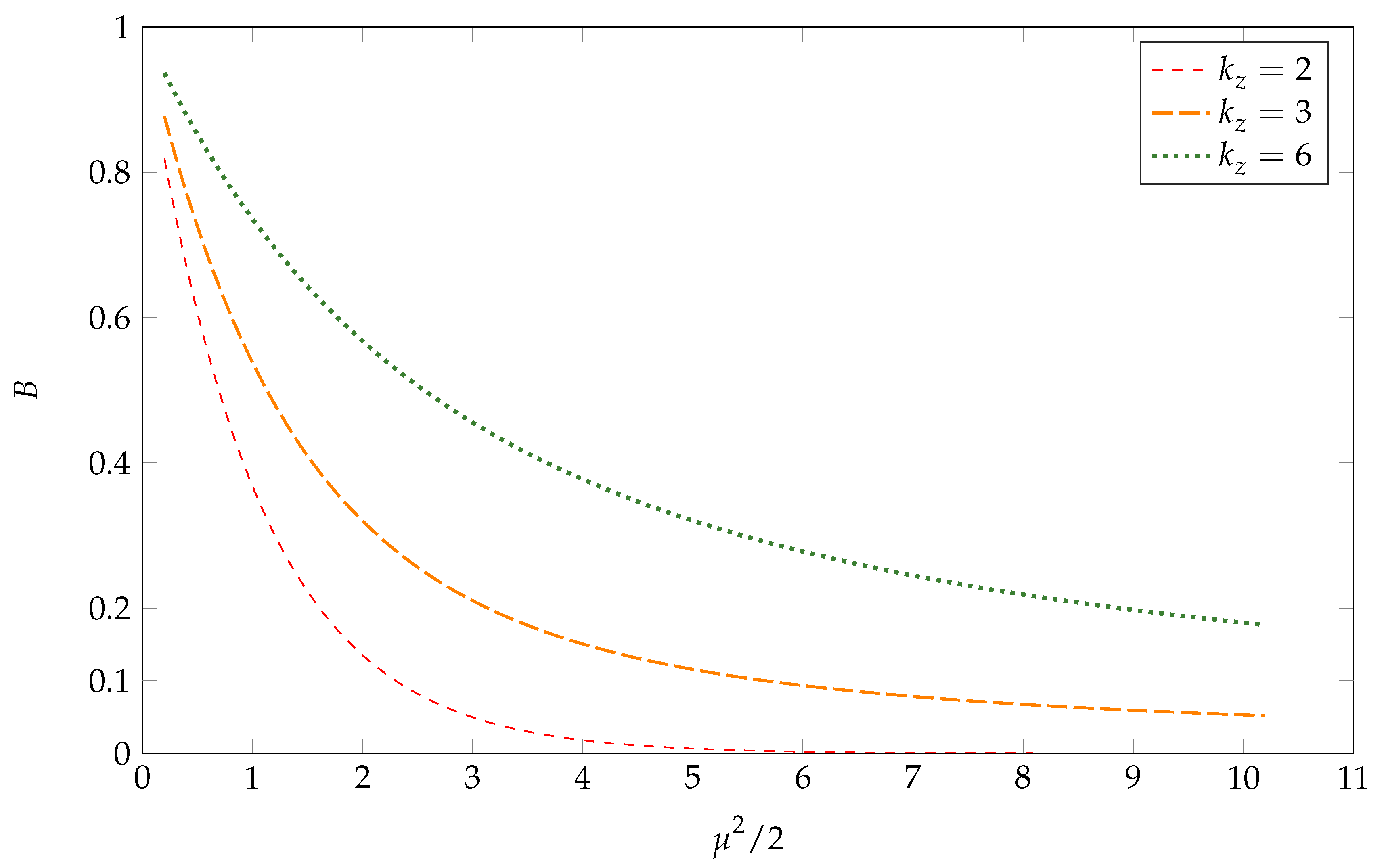
The values of the limiting relative biases of and are explored in Figure 1 for different values of the parameters and . The figure illustrates that, for , the function is increasing in its argument, which is . Note also that, as , the information in the instruments approaches zero, and so the local-to-zero asymptotic bias of approaches that of from below. Hence, the limit of the relative asymptotic biases at is unity, which is the value of .
Remark 3.
Theorem 2.
The critical values are decreasing functions of B for given .
Proof.
See Appendix B.2. □
Heuristically, Theorem 2 states that the critical values will necessarily decrease as one moves from left to right across any given row of Table 1; that is, the critical values decrease as the practitioner is willing to accept increasing amounts of 2SLS bias relative to that of OLS. The intuition behind the results is as follows. An increase in B for fixed implies that the argument of the confluent hypergeometric function in (9) must increase, i.e., that must decrease. As approaches zero, the non-central chi-squared distribution from which critical values are drawn approaches a central chi-squared and the corresponding quantiles become smaller. Hence, as one moves across columns from left to right in Table 1, the become smaller.
Theorem 2 explains the row behaviour of Table 1. Explaining the column behaviour is much more complicated. Observation suggests the following to be true.
Conjecture 1.
For given B, the critical values , presented in Table 1, are increasing functions of up to some value, k say, whereafter they are decreasing functions of . k is a decreasing function of B.
Some intuition for Conjecture 1 is available from the definition of , see (5), if one considers the impact of increasing the number of instruments by one, from to , with superscripts ‘0’ and ‘1’ distinguishing the two cases, respectively. For given B and ,
k is then that value of after which the start diminishing.
Remark 4.
Although B does not exist when , the confluent hypergeometric function of Theorem 1 remains well-defined. In Appendix D, we analyse the properties of .
4. Some Monte Carlo Results
We follow Sanderson and Windmejer (2016) and specify the model is as in (1) and (2), with and
The instruments in Z are independent standard normally distributed random variables and , where is a vector of ones, and with chosen such that the relative bias B is equal to , , or , for values of and . The sample size 10,000 and the results are presented in Table 3 for 100,000 Monte Carlo replications.
For , the results are exactly in line with the theory: the Monte Carlo relative biases are equal to B and the rejection frequencies of the first-stage F-test are 5% at the 5% nominal level, using the critical values reported in Table 1.
The results for are also in line with the theory, although we see here that the standard deviations of are much larger than those of the case at the same values of B. This is due to the fact that the information needed to obtain the same relative bias is much smaller for the case than for the case, as reflected by their smaller values, but it also reflects the problem that the second moment does not exist when the degree of over-identification is equal to 1. The interquartile ranges for the 2SLS estimator when are and for and , respectively. These Monte Carlo results therefore confirm our theoretical findings for the case. Clearly some caution should be exercised when working with 2SLS in this case because it possesses no second moment.
5. -Values
p-values are readily available as a straightforward extension of our earlier analysis. Specifically, from (4), we have the limiting result
For any particular sample value of the F-test, say , if then the p-value for the SY weak instruments test considered in this paper is simply . Of course, the problem here is the determination of . Table 4 reports those values of that were calculated in order to construct Table 1. For those values of B considered in Table 1, we now have the parameters and . Consequently, any computer software that can evaluate a non-central chi-squared cdf can readily calculate p-values for the test for weak instruments considered here.
6. Multiple Endogenous Regressors
The general case is obtained by defining x in (1) to be a matrix of endogenous regressors of dimension , say, so that is . Then, (2) becomes a multivariate regression model with of dimension and v of dimension . The rows of are independent with common covariance matrix . All other aspects of the model described in (1) and (2) remain essentially unchanged.11
In terms of the SY analysis, it clearly makes no sense to proceed in terms of the ratio
given that is now a vector rather than a scalar quantity. Thus, instead, they focus attention on the quadratic form (SY, Equation 3.8)
where h is a matrix analogue of the expectation explored in Theorem 1 and , with defined in SY (p. 85). The essential feature of is that it is not a function of . Despite being somewhat more tractable, the quadratic form tells us no more about the non-centrality parameter determining the bias of the 2SLS estimator than does
say, where the elements of the matrix are jointly distributed according to
with as defined in SY (p. 85).12 Again, we should stress that the normality of is a consequence of the local-to-zero asymptotic analysis and is not a strong distributional assumption. As is independent of , it is sufficient to focus attention on the vector of expectations . If we let denote the ith row of the identity matrix then we have immediately13
where the ith element of the vector is , with .14 Here, denotes ordered partitions of j into no more than parts, so that where the integers satisfy the restrictions (i) , (ii) , and (iii) . The symbol then denotes the sum over all such partitions of j. For example, the ordered partitions of 2 are the so-called top partition and .15 The invariant polynomials and the symbol are defined in Davis (1979), p. 465, with a constant that may be zero. These were developed as extensions (to two matrix arguments) of the zonal polynomials originally due to James (1961).16 Finally, the generalised hypergeometric coefficients are defined as (Constantine 1963 Equation (26))
where , is the usual Pochhammer symbol or forward factorial (see Slater 1966, Appendix I).
Expressions like (14) are computationally problematic. The available evidence suggests that the series are typically slow to converge (Phillips 1983a, 1983b). Unfortunately, the invariant polynomials of Davis are tabulated only to low order and, to date, no algorithms have been derived for their computation.17 Consequently, until such time as the computational restrictions are lifted, the practical relevance of the result is limited and is offered here only for completeness. Better progress might be made working with one of the various approximation techniques that are available, e.g., the Laplace approximation used by Phillips (1983b) to extract approximate marginal distributions for IV estimators in this more general setting. In this case, however, we can further adapt the results of Hillier et al. (1984) to obtain many instrument approximations to (14). Specifically, analogous to their Equations (32) and (33), we have
and
where denotes the ith element of .18
Although these approximations are operational, in the presence of multiple endogenous regressors, we question whether the approach of SY is as sound as it is in the single endogenous regressor case. Our concern is rooted in the structure of the Davis polynomials themselves. For matrix arguments, X and Y with given indices k and l, respectively, the polynomials are ‘linear combinations of the distinct products of traces
of total degree k, l in the elements of X, Y, respectively (Davis 1979, p. 468). It is immediately apparent that local-to-zero asymptotic expression for the bias of 2SLS is not a function of the eigenvalues of the concentration parameter or, at least, not a function of them alone. Stock and Yogo (2005), p. 90, remark on this themselves when discussing certain numerical results, where they observe that 2SLS bias is decreasing in all eigenvalues of the concentration parameter for all values of (what we call) . To focus on the smallest eigenvalue, as the Cragg–Donald statistic does, is, consequently, problematic. Another way of thinking of this problem is to consider the problem of determining the magnitude of a matrix and to ask which of the following three matrices is either largest or smallest:
While consideration of the smallest eigenvalue will lead to a particular choice, it is not clear that that choice actually has that much to do with the exact behaviour of the IV estimator, except in the scalar case. Indeed, for this reason, the SY results for multiple endogenous variable cases are only approximate and provide upper bounds on critical values for the Cragg–Donald minimum eigenvalue test. That the SY approach works in the case of a single endogenous regressor is a consequence of the commutative law of multiplication that allows us to extract scalars from products in ways that we can’t in more general matrix situations. In summary, the SY approach results in a well-posed problem in the case of a single endogenous regressor but a somewhat poorly-posed problem in the case of multiple endogenous regressors.
If one must deal with multiple endogenous regressors, then we prefer the approach of Sanderson and Windmejer (2016), who define weak identification as the rank of being local to a rank reduction of one, which is essentially a scalar problem. By reducing the problem in this way, the approach is reduced to a well-posed problem for which the single endogenous variable results apply, only the degrees of freedom need to be adjusted for the number of endogenous variables (see Sanderson and Windmejer (2016) for details).
7. The Wisdom of Hindsight: Some Historical Remarks
As discussed in Footnote 7, helpful referees drew our attention to the fact that there are other ways that we might have approached this problem than the one that we initially chose. Indeed, once one recognises the the structure of the problem, many results become available. However, before discussing some of these, we will again stress that the results derived in the previous sections are all asymptotic in nature, there are no underlying exact distributional assumptions beyond those originally made in Staiger and Stock (1997). What these results share with the exact distribution literature is integrals with similar structures and a common approach to resolving them. Furthermore, the parameterisations adopted here are different from the canonical forms underlying the exact distributional results and so the resultant expressions are different even if their structures are reminiscent of earlier results. A prime example of this is given by the similarities between the many, local-to zero, instrument approximations of Equations (15) and (16) and the large-sample approximations of (Hillier et al. (1984, Equations (32) and (33)).
It was noted in Footnote 7 that Chao and Swanson (2007) had derived local-to-zero asymptotic expressions for the bias of both 2SLS and OLS in the scalar case, so that they might bias correct the estimators, and that these provide an alternate path to Theorem 1. If moments were the focus of our attention, then we should note that the results of Chao and Swanson (2007) have the same structure as do those of Richardson (1968) and references cited therein, who first derived moments in the scalar case with arbitrary numbers of instruments and proved Basmann’s conjecture (Richardson 1968, Section 4.3) for the existence of moments. In the general case, we should, of course, be looking to Hillier et al. (1984) for results with the same structure as presented here and to Kinal (1980), who established existence criteria in the general case. Noting that the distributions of interest in the exact finite sample literature are different from the distributions thrown up by the local-to zero asymptotics, with different parameters, it might be argued that the exact results for misspecified models are closer in spirit to what we have here. In this event, we might argue that results for moments are implicit (but unrecognisable) in Hale et al. (1980) or, in a far more recognisable form in Knight (1982), for the scalar case, or Skeels (1995) in the general case. However, here moments are only of interest as an intermediate result to obtain the relative bias that is used to obtain a non-centrality parameter that determines the non-central chi-squared distribution of interest in step 3 of the procedure given following (8). Perhaps of greater historical interest, in the scalar case, are the results of Richardson and Wu (1971) who explore the properties of the relative bias. However, these results are of limited interest for two reasons. First, and probably most important, because the parameterisation of their model differs from that generated by the local-to-zero asymptotics, their tabulated results are not comparable with what is done here. Second, to reiterate, the relative bias is only of interest to us inasmuch as it allows us, given certain other information, to chose a non-centrality parameter useful in determining SY critical values in the scalar case. That is, unlike for all of the above-mentioned papers, moments are only of tangential interest to us, as this is not a study of the estimators themselves. To the best of our knowledge, Section 6 provides the first treatment of the (local-to-zero asymptotic) relative bias in the general case.
8. Conclusions
The main contribution of this paper has been to resolve analytically an integral as a special function, obviating the need to resolve it by simulation. This integral is of independent interest in the theory of ratios of quadratic forms in normal variables. Here, it is of primary interest because it provides a functional relationship between the bias in the 2SLS estimator and the limiting sampling distribution of a test statistic that SY proposed for testing the presence of weak instruments, when the null of weak instruments is true. Analysis of this special function provides theoretical foundations for the remarks of Section 3, which explore patterns observed in Table 1 as the parameters B and vary. This analysis required the derivation of certain results that are of independent interest in the theory of confluent hypergeometric functions. We have also explored the problem of p-values of the aforementioned test for weak instruments, on the basis of our earlier theoretical developments. We provide information such that any computer software that can then evaluate a non-central chi-squared cdf can readily compute p-values in essentially all practical circumstances. The final contribution of this paper has been the analysis of the general case characterised by an arbitrary number of endogenous regressors. Here, we find that the analysis is able to draw heavily on the foundations laid down in the literature on exact sampling distributions. This allows us to provide expressions for both the expectation of interest and also first- and second-order many-instrument expansions of this expectation. The exact expression obtained for the integral of interest in the general case is not of great practical interest, as it involves invariant polynomials with two matrix arguments for which, at the time of writing, there exist no algorithms for their computation, except in special cases. Nevertheless, the asymptotic expansions obtained are readily computable and potentially of practical importance. Given our reservations about the usefulness of the overall procedure in the general case, we leave such explorations to others.
One aspect of the SY tables that we have not addressed relates to those tables based on size distortions of a Wald statistic. This is a much more difficult analytical problem than has been addressed here and it is not clear that there is much benefit in tackling it as, in our estimation, the bias tables are in much more frequent use, making them of greater practical relevance.
Finally, in support of the results presented in the paper, we provide two Matlab programs on an ‘as is’ basis. The first of these, Table1.m, provides the body of Table 1. The second program, entitled sypval.m, provides p-values. Appendix C provides some discussion on the contents of these programs. The programs are available at https://sites.google.com/site/skeelscv/.
Author Contributions
F.W. conceived, designed, and performed the simulation experiments; C.S. and F.W. wrote the paper.
Funding
Windmeijer acknowledges funding from the Medical Research Council (MC_UU_12013/9).
Acknowledgments
We happily acknowledge our intellectual debt to Peter Phillips, whose seminal contributions to the analysis of inference in simultaneous equations models is but a small part of his enormous contribution to the econometrics literature over a nearly 50-year period. We are particularly grateful to Grant Hillier for helping us with some technical details that form the basis of Appendix E. We also acknowledge Jon Temple, who provided extensive comments on an earlier draft of this paper, and Mark Schaffer for more recent comments. We would also like to thank the anonymous referees for their very constructive comments. The usual caveat applies. Skeels thanks the Department of Economics at the University of Bristol for their hospitality during his visits there, which is where this paper was first written. Finally, we would like to dedicate this paper to the memory of John Knight, a fine scholar and, far more importantly, one of nature’s true gentlemen, taken far too soon.
Conflicts of Interest
The authors declare no conflict of interest.
Appendix A. The Expectation of a Particular Function of Normal Random Variables
Theorem A1.
Suppose that . Then,
where .
Proof.
It is straightforward to demonstrate that the expectation is unbounded when and so we shall assume hereafter that . Given the normality assumption on , we can write
In accordance with Herz (1955), Lemma 1.4, we can decompose almost all k-vectors into , where , so that , and , with volume elements
This is essentially a transformation to polar coordinates. The resulting expression is
almost everywhere. Next, write
and evaluate the integrals over using Hillier et al. (1984), Equation (6):
This yields, on replacing by ,
where denotes a generalised hypergeometric function. Finally, differentiating with respect to t, using say NIST (2015, Equation 16.3.1), evaluating the derivative at , and then resolving the resulting Laplace transforms using
yields
where the second to last equality exploits one of the relationships for contiguous confluent hypergeometric functions (NIST 2015, Equation 13.3.4) and the final equality is another application of Kummer’s transformation. □
Appendix B. Analysis of Table 1
Appendix B.1. Preliminaries
In this appendix, we analyse how the critical values , presented in Table 1, change in response to changes in one of either or B when the other is held fixed; that is, as one either moves down columns of the table or across rows, from left to right, respectively. Some additional analysis is available in Skeels and Windmeijer (2016).
From Equation (5),
with the solution to the equation
where denotes the density function of a non-central chi-squared random variable; specifically
where
The parameter is chosen to satisfy
The absolute values can be ignored as the confluent hypergeometric function is positive for all whenever , which shall be assumed for the rest of this appendix unless indicated otherwise.
Appendix B.2. The Consequence of Varying B for Fixed
With held fixed we have, from (A4),
First,
for all and . Second, using Leibniz’s Rule for the differentiation of integrals, we can differentiate both sides of (A5) with respect to to obtain,
Note that (A11) implicitly assumes , so that . In the event that either or is infinite, then , as does its derivative with respect to , making the representation (A11) invalid. Indeed, as these cases are on the boundaries of support of a non-central chi-squared random variable, the ordinary derivative is not well-defined and so the approach taken above would require modification. For this reason, hereafter, we shall assume that .
Integrating by parts allows us to write
and so (A11) becomes
as . The positivity of the ratio follows because each of the functions f are values of non-central chi-squared density functions which differ only in their degrees of freedom, versus respectively, and so are both everywhere positive for all , as is assumed above. As an aside, we know that as degrees of freedom increase for given these functions cross, which means that sometimes and sometimes the converse is true. That is, we are unable to bound from above.
Appendix C. Some Remarks on Computational Aspects
For the most part, both the programs Table1.m and sypval.m rely on intrinsic Matlab functions. Once the relevant inputs are available then the structure of the programs is immediately apparent. Specifically, for given values of and B, it is necessary to obtain the corresponding value for from the nonlinear Equation (9). We adopt a fairly simple-minded approach to this, by iterating from a starting value to the correct solution using a bisection algorithm.
Our starting values are chosen as follows. When , we know from (10) that the values of can be calculated exactly as and so no search is required. When we exploit an approximation asymptotic in (Slater 1960, Equation (4.1.8)) that reduces to . As expected, the performance of the approximation improves as B decreases which, for fixed , corresponds to increasing (see Appendix B.2). Nevertheless, for all cases where , this approximation provides much better starting values in the search for than do naive alternatives, such as starting the search from zero (say). Moreover, this approximation performs best under exactly the same circumstances that naive methods are at their slowest, affording considerable computational time savings. As the values of are much more stable for any given B than the , as can be deduced from Table 4, we use this parameterisation in our search algorithm.
Appendix D. Some Remarks on the Just-Identified Scalar Case
The SY approach is not available if because the bias of 2SLS does not exist, hence is undefined.19 Nevertheless, given the difficulties often encountered in finding appropriate instruments, the exactly identified model is one of considerable practical relevance. As the confluent hypergeometric function of Theorem 1 remains well-defined when , one might ask if it could provide an ad hoc basis for a test for weak instruments in this case, based on F, in the spirit of the SY approach.
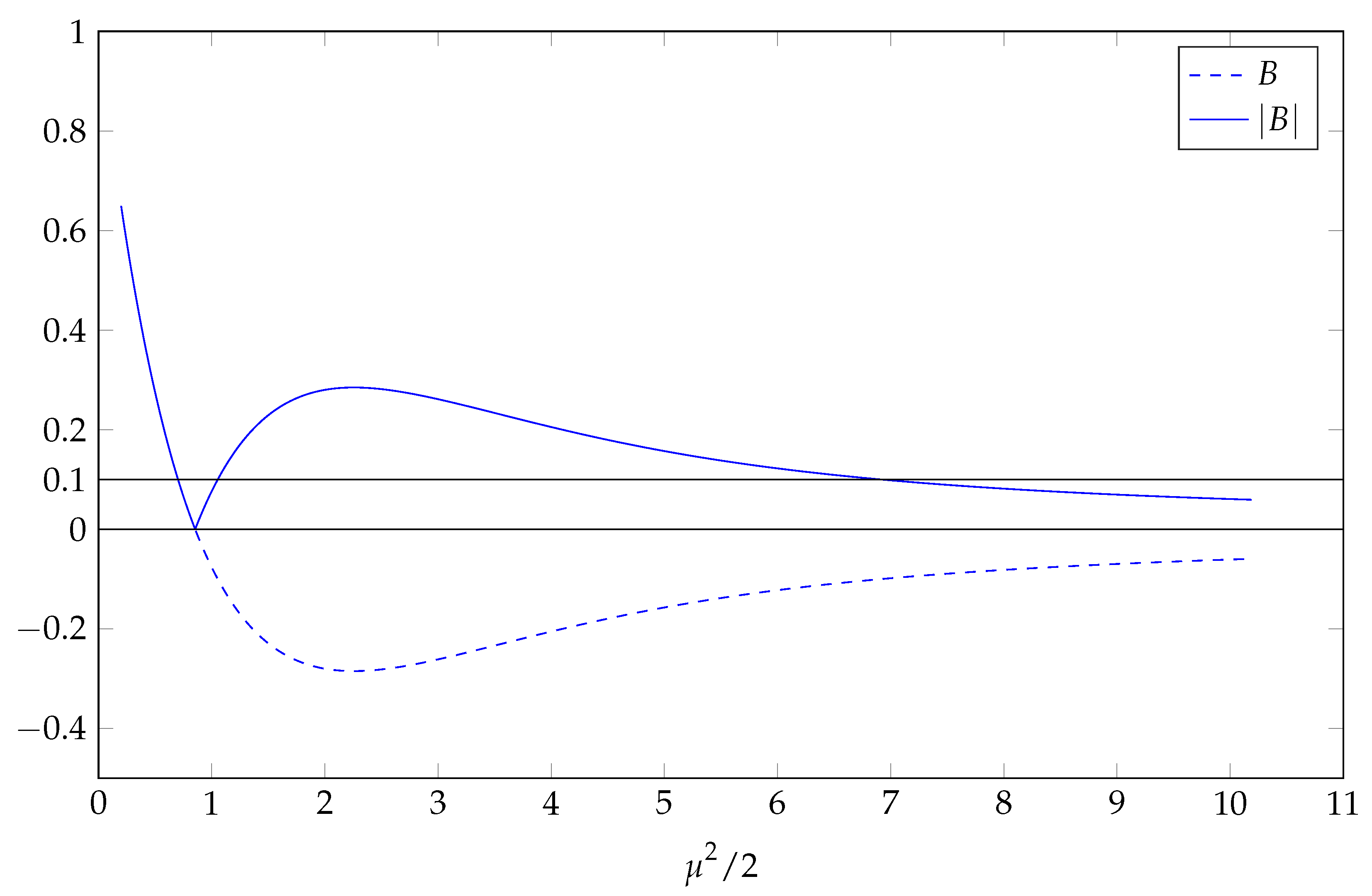
The function displays behaviours that are quite different to what was observed in over-identified models. These behaviours are displayed in Figure A1 where we plot both the confluent hypergeometric function and its absolute value against , when . Note that in the figure we use the symbol B to represent the confluent hypergeometric function , rather than the expectation , with the latter unbounded when .
In Figure A1, we see that neither B nor are monotonic in when , in contrast to the over-identified cases. That the confluent hypergeometric function can take negative values when means that this case is the only one considered where taking the absolute value of the hypergeometric function has any material impact on observed behaviour. We can establish numerically that B, and hence , both have a zero at . As this is in the region where the hypergeometric function is a decreasing value of its argument, we see that, as B moves through its zero to the right, so that is increasing, it becomes negative and appears to stay that way, with a minimum of approximately occurring at . Clearly, cannot become negative and so, at , it has a local maximum of approximately . Consequently, there are three values of that yield the same value of for , there are two values of corresponding to , and for there is a one-to-one mapping between and .
Figure A1.
Plots of and its absolute value against .

Observe in Figure A1 that there are three values of corresponding to . Setting , the largest of these numbers, we find a critical value for the first-stage F-test of 28.77. At this level of information, the 2SLS estimator appears well-behaved. This is shown in Table A1, which shows the estimation result of a Monte Carlo analysis as in Section 4 for . Even though it has no moments as the model is just-identified, we find that the Monte Carlo relative bias is indeed 10% with the rejection frequency of the F-test again 5%. The same holds at the smaller values of of 0.05 and 0.01, for which the largest implied values of are 23.41 and 103.06, with the estimation results very similar to those for . However, when we consider the case, for which is 8.198, the lack of moments of the 2SLS estimator becomes apparent, with the standard deviation now very large at 6.05. These results suggest that the approximation might be useful for the smaller values of , if one works with the largest implied values of , even though the 2SLS estimator does not possess any moments in this case.

Table A1.
Simulation results for .
| B | ||||||||
|---|---|---|---|---|---|---|---|---|
| −0.01 | −0.05 | −0.10 | −0.20 | |||||
| mean | std dev | mean | std dev | mean | std dev | mean | std dev | |
| 1.4949 | 0.0086 | 1.4988 | 0.0086 | 1.4993 | 0.0086 | 1.4996 | 0.0087 | |
| 0.9954 | 0.1003 | 0.9753 | 0.2327 | 0.9495 | 0.4389 | 0.8936 | 6.0492 | |
| F | 104.11 | 20.411 | 24.429 | 9.8352 | 14.821 | 7.5732 | 9.1757 | 5.8671 |
| −0.0092 | −0.0496 | −0.1011 | −0.2130 | |||||
| 103.06 | 23.412 | 13.830 | 8.198 | |||||
| cv F | 139.17 | 42.035 | 28.769 | 20.323 | ||||
| rej freq F | 0.0496 | 0.0507 | 0.0485 | 0.0489 | ||||
Notes: Sample size n = 10,000, number of Monte Carlo replications is 100,000.
Confirming the approximate median unbiasedness of the just-identified 2SLS estimator (see, for example, the discussion in Angrist and Pischke (2009), p. 209), we find that the median biases, not reported in the table, are very close to 0 at all values of .
Appendix E. Derivation of the O() Term in (16)
The following derivation is due to Grant Hillier, via private communication, and we thank him for allowing us to include it here.
By analogy with Hillier et al. (1984), Equation (31), the term in (16) requires the resolution of an integral of the form
where denotes the ith column of an identity matrix, , with , and the range of integration is the set of complex, symmetric matrices of dimension with fixed, positive definite real part. Noting that
where and are the non-zero eigenvalues of , and and are the corresponding eigenvectors, respectively. Making this substitution, the integral of interest reduces a weighted sum of integrals of the form , where
We shall present the key result in the following lemma.
Lemma A1.
Let W be a complex, symmetric matrix whose real part is fixed and positive definite, i.e., , let S denote a non-singular, symmetric matrix of the same dimension, and let η denote a fixed p-vector. Then, the inverse Laplace transform of
is
Proof.
Noting that
we see that is times the coefficient on in
That is,
The hypergeometric function in (A15) has the integral representation (James 1961, Theorem 5)
where denotes the normalised invariant Haar measure on the unit sphere, and so
where
is symmetric and positive definite for small enough t,and the final equality in (A15) follows from Muirhead (1982), pp. 252–53. Now
say, where and . Hence,
Applying Lemma A1 to (A14), and re-combining the spectral decomposition, we find that
Equation (16) follows directly on substituting for .
References
- Angrist, Joshua D., and Jörn-Steffen Pischke. 2009. Mostly Harmless Econometrics. An Empiricist’s Companion. Princeton and Oxford: Princeton University Press. [Google Scholar]
- Baum, Christopher F., Mark E. Schaffer, and Steven Stillman. 2010. ivreg2: Stata Module for Extended Instrumental Variables/2SLS, GMM and AC/HAC, LIML, and k-Class Regression. Boston College Department of Economics, Statistical Software Components S425401. Available online: http://ideas.repec.org/c/boc/bocode/s425401.html (accessed on 26 August 2015).
- Buse, Adolf. 1992. The bias of instrumental variables estimators. Econometrica 60: 173–80. [Google Scholar] [CrossRef]
- Chao, John, and Norman R. Swanson. 2007. Alternative approximations of the bias and MSE of the IV estimator under weak identification with an application to bias correction. Journal of Econometrics 137: 515–55. [Google Scholar] [CrossRef]
- Cohen, Jonathan D. 1988. Noncentral Chi-Square: Some observations on recurrence. The American Statistician 42: 120–22. [Google Scholar] [CrossRef]
- Constantine, A. Graham. 1963. Some non-central distribution problems in multivariate analysis. Annals of Mathematical Statistics 34: 1270–85. [Google Scholar] [CrossRef]
- Cragg, John G., and Stephen G. Donald. 1993. Testing identifiability and specification in instrument variable models. Econometric Theory 9: 222–40. [Google Scholar] [CrossRef]
- Das Gupta, Somesh, and Michael D. Perlman. 1974. Power of the noncentral F-test: Effect of additional variates on Hotelling’s T2-test. Journal of the American Statistical Association 69: 174–80. [Google Scholar]
- Davis, A. William. 1979. Invariant polynomials with two matrix arguments extending the zonal polynomials: Applications to multivariate distribution theory. Annals of the Institute of Statistical Mathematics 31 Pt A: 465–85. [Google Scholar] [CrossRef]
- Dufour, Jean-Marie. 1997. Some impossibility theorems in econometrics with applications to structural and dynamic models. Econometrica 65: 1365–87. [Google Scholar] [CrossRef]
- Forchini, Giovanni, and Grant H. Hillier. 2003. Conditional inference for possibly unidentified structural equations. Econometric Theory 19: 707–43. [Google Scholar] [CrossRef]
- Hale, Christopher, Roberto S. Mariano, and John G. Ramage. 1980. Finite sample analysis of misspecification in simultaneous equation models. Journal of the American Statistical Association 75: 418–27. [Google Scholar] [CrossRef]
- Herz, Carl S. 1955. Bessel functions of matrix argument. Annals of Mathematics 61: 474–523. [Google Scholar] [CrossRef]
- Hillier, Grant H., Raymond Kan, and Xiaolu Wang. 2009. Computationally efficient recursions for top-order invariant polynomials with applications. Econometric Theory 25: 211–42. [Google Scholar] [CrossRef]
- Hillier, Grant H., Raymond Kan, and Xiaolu Wang. 2014. Generating functions and short recursions, with applications to the moments of quadratic forms in noncentral normal vectors. Econometric Theory 30: 436–73. [Google Scholar] [CrossRef]
- Hillier, Grant H., Terrence W. Kinal, and Virendra K. Srivastava. 1984. On the moments of ordinary least squares and instrumental variables estimators in a general structural equation. Econometrica 52: 185–202. [Google Scholar] [CrossRef]
- James, Alan T. 1961. Zonal polynomials of the real positive definite symmetric matrices. Annals of Mathematics 74: 456–69. [Google Scholar] [CrossRef]
- James, Alan T. 1964. Distributions of matrix variates and latent roots derived from normal samples. The Annals of Mathematical Statistics 35: 475–501. [Google Scholar] [CrossRef]
- Johansson, Fredrik. 2016. Computing Hypergeometric Functions Rigorously. Available online: https://hal.inria.fr/hal-01336266v2 (accessed on 15 September 2016).
- Kinal, Terrence W. 1980. The existence of moments of k-class estimators. Econometrica 49: 241–49. [Google Scholar] [CrossRef]
- Kleibergen, Frank. 2002. Pivotal statistics for testing structural parameters in instrumental variables regression. Econometrica 70: 1781–803. [Google Scholar] [CrossRef]
- Knight, John L. 1982. A note on finite sample analysis of misspecification in simultaneous equation models. Economics Letters 9: 275–79. [Google Scholar] [CrossRef]
- MathWorks. 2016. MATLAB and Statistics Toolbox Release 2016b. Natick: The MathWorks Inc. [Google Scholar]
- Muirhead, Robb J. 1982. Aspects of Multivariate Statistical Theory. New York: John Wiley and Sons, Inc. [Google Scholar]
- National Institute of Standards and Technology (NIST). 2015. Digital Library of Mathematical Functions; Edited by Frank W. J. Olver, Adri B. Olde Daalhuis, Daniel W. Lozier, Barry I. Schneider, Ronald F. Boisvert, Charles W. Clark, Bruce R. Miller and Bonita V. Saunders. Release 1.0.10 of 2015-08-07; Gaithersburg: NIST. Available online: http://dlmf.nist.gov/ (accessed on 10 August 2015).
- Nelson, Charles R., and Richard Startz. 1990a. The distribution of the instrumental variables estimator and its t-ratio when the instrument is a poor one. Journal of Business 63 Pt 2: S125–40. [Google Scholar] [CrossRef]
- Nelson, Charles R., and Richard Startz. 1990b. Some further results on the exact small sample properties of the instrumental variable estimator. Econometrica 58: 967–76. [Google Scholar] [CrossRef]
- Phillips, Peter C. B. 1980. The exact distribution of instrumental variable estimators in an equation containing n + 1 endogenous variables. Econometrica 48: 861–78. [Google Scholar] [CrossRef]
- Phillips, Peter C. B. 1983a. Exact small sample theory in the simultaneous equations model. In Handbook of Econometrics, Volume I. Edited by Zvi Griliches and Michael D. Intriligator. Amsterdam: North Holland, Chapter 8. pp. 449–516. [Google Scholar]
- Phillips, Peter C. B. 1983b. Marginal densities of instrumental variable estimators in the general single equation case. Advances in Econometrics 2: 24. [Google Scholar]
- Phillips, Peter C. B. 1989. Partially identified econometric models. Econometric Theory 5: 181–240. [Google Scholar] [CrossRef]
- Phillips, Peter C. B. 2016. Inference in near-singular regression. Advances in Econometrics 36: 461–86. [Google Scholar] [CrossRef]
- Phillips, Peter C. B. 2017. Reduced forms and weak instrumentation. Econometric Reviews 36: 818–39. [Google Scholar] [CrossRef]
- Phillips, Peter C. B, and Wayne Y. Gao. 2017. Structural inference from reduced forms with many instruments. Journal of Econometrics 199: 96–116. [Google Scholar] [CrossRef]
- Richardson, David H. 1968. The exact distribution of a structural coefficient estimator. Journal of the American Statistical Association 63: 1214–26. [Google Scholar] [CrossRef]
- Richardson, David H., and De-Min Wu. 1971. A note on the comparison of ordinary and two-stage least squares estimators. Econometrica 39: 973–81. [Google Scholar] [CrossRef]
- Sanderson, Eleanor, and Frank Windmejer. 2016. A weak instrument F-test in linear IV models with multiple endogenous variables. Journal of Econometrics 190: 212–21. [Google Scholar] [CrossRef] [PubMed]
- Skeels, Christopher L. 1995. Instrumental variables estimation in misspecified single equations. Econometric Theory 11: 498–529. [Google Scholar] [CrossRef]
- Skeels, Christopher L., and Frank Windmeijer. 2016. On the Stock–Yogo Tables. Discussion Paper 16/679. Bristol: Department of Economics, University of Bristol. [Google Scholar]
- Slater, Lucy J. 1960. Confluent Hypergeometric Functions. Cambridge: Cambridge University Press. [Google Scholar]
- Slater, Lucy J. 1966. Generalized Hypergeometric Functions. Cambridge: Cambridge University Press. [Google Scholar]
- Staiger, Douglas, and James H. Stock. 1997. Instrumental variables regression with weak instruments. Econometrica 65: 557–86. [Google Scholar] [CrossRef]
- StataCorp. 2015. Stata Statistical Software: Release 14. College Station: StataCorp LP. [Google Scholar]
- Stock, James H., and Motohiro Yogo. 2005. Testing for weak instruments in linear IV regression. In Identification and Inference for Econometric Models: Essays in Honor of Thomas Rothenberg. Edited by Donald W. K. Andrews and James H. Stock. Cambridge: Cambridge University Press, Chapter 5. pp. 80–108. [Google Scholar]
- Wasserstein, Ronald L., and Nicole A. Lazar. 2016. The ASA’s statement on p-values: Context, process, and purpose. The American Statistician 70: 129–33. [Google Scholar] [CrossRef]
| 1. | Much of the later literature has focussed less on testing for the presence of weak instruments and more on the development of techniques that are robust to the presence of weak instruments. |
| 2. | A heuristically appealing aspect of using the first-stage F-statistic as a measure of instrument weakness, in the case of a single endogenous regressor, is its consistency with the well-known Staiger–Stock rule of thumb. Staiger and Stock (1997), p. 557, suggested that instruments be deemed weak if the first-stage F is less than 10. SY (pp. 101–2) observe that 10 corresponds closely to their tabulated critical values for a 5% test that the relative bias is 10% for all values of , and concluded that ‘this provides a formal, and not unreasonable, testing interpretation of the the Staiger–Stock rule of thumb.’ |
| 3. | Through the use of more extensive simulation results than those used originally by SY, we are able to support the proposition that the numerical approximation errors inherent in the computation of our analytical results are less than those contained in the original SY tables. |
| 4. | Some references specify the non-centrality parameter for a non-central chi-squared distribution as , whereas others specify it as . We have adopted the former convention here. |
| 5. | The exact details of these arguments can be found in SY and will not be repeated here. |
| 6. | We thank an anonymous referee for bringing this subtlety to our attention. For a more complete discussion of this point, we refer the reader to the discussion of (Chao and Swanson 2007, pp. 518–19) and the references cited therein. |
| 7. | It should be noted that the proof provided is not the only one possible and we would like to thank helpful referees for drawing various alternatives to our attention. For example, in an elegant paper, Chao and Swanson (2007), Proposition 3.1 and Lemma 3.3, respectively, derive local to zero approximations for each of and , from whence derivation of the ratio is straightforward. Similarly, there are finite sample papers in the literature from which it would be possible to start a proof along the lines of the one presented but at a more advanced point (see, for example, Forchini and Hillier 2003, Equation B.13). However, we favour the proof presented for two reasons. First, it is a direct continuation of the developments of Stock and Yogo (2005), Equation 3.1, and the discussion immediately thereafter. Second, when viewed in the correct light, there are much earlier antecedents that take precedence over the two mentioned here. We discuss this further in Section 6. |
| 8. | |
| 9. | We have also computed simulated critical values from 20,000 random draws as in SY, but repeating the exercise 1000 times. The resulting mean critical values are virtually identical to those in Table 1, with the maximum difference being 0.02. |
| 10. | Theorem 2 is similar in spirit to Das Gupta and Perlman (1974), p. 180, Remark 4.1, although they only address the numerator of the ratio in Equation (5). Consequently, Das Gupta and Perlman are silent on the relative magnitudes of and which, in essence, is the content of Theorem 2. |
| 11. | The complete set of assumptions are presented in SY (Section 2.4). |
| 12. | |
| 13. | Make the substitutions for , respectively, in Hillier et al. (1984), Equation (30). |
| 14. | Please note that the definition of adopted here is slightly different from the definitions used in either Hillier et al. (1984) and SY. |
| 15. | |
| 16. | The zonal polynomials appearing in (14) adopt a normalisation due to Constantine (1963), which typically leads to more compact expressions than do the polynomials originally proposed by James (1961). |
| 17. | Some progress towards addressing the computational aspects of these polynomials has been made by Hillier et al. (2009, 2014). |
| 18. | Although the derivation of (15) is straightforward, this is less true for (16). A derivation of the terms in (16) that are in addition to those in (15) is provided in Appendix E. |
| 19. | Similarly, in the proof of Theorem A1, we established that was unbounded when . |
| 20. |
Figure 1.
Plots of against for and 6.

Table 1.
5% Critical values for single endogenous regressor, 2SLS bias.
| 0.01 | 0.05 | 0.1 | 0.15 | 0.2 | 0.25 | 0.3 | |
|---|---|---|---|---|---|---|---|
| 2 | 11.57 | 9.02 | 7.85 | 7.14 | 6.61 | 6.19 | 5.83 |
| 3 | 46.32 | 13.76 | 9.18 | 7.52 | 6.60 | 5.96 | 5.49 |
| 4 | 63.10 | 16.72 | 10.23 | 7.91 | 6.67 | 5.88 | 5.32 |
| 5 | 72.55 | 18.27 | 10.78 | 8.11 | 6.71 | 5.82 | 5.19 |
| 6 | 78.59 | 19.19 | 11.08 | 8.21 | 6.70 | 5.75 | 5.09 |
| 7 | 82.75 | 19.79 | 11.25 | 8.25 | 6.67 | 5.69 | 5.01 |
| 8 | 85.78 | 20.20 | 11.36 | 8.26 | 6.64 | 5.63 | 4.93 |
| 9 | 88.07 | 20.49 | 11.42 | 8.25 | 6.60 | 5.58 | 4.87 |
| 10 | 89.86 | 20.70 | 11.46 | 8.24 | 6.56 | 5.52 | 4.81 |
| 11 | 91.30 | 20.86 | 11.49 | 8.22 | 6.53 | 5.48 | 4.76 |
| 12 | 92.47 | 20.99 | 11.50 | 8.20 | 6.49 | 5.43 | 4.71 |
| 13 | 93.43 | 21.08 | 11.50 | 8.17 | 6.46 | 5.39 | 4.67 |
| 14 | 94.25 | 21.16 | 11.50 | 8.15 | 6.42 | 5.36 | 4.63 |
| 15 | 94.94 | 21.22 | 11.49 | 8.13 | 6.39 | 5.32 | 4.59 |
| 16 | 95.54 | 21.26 | 11.49 | 8.11 | 6.36 | 5.29 | 4.56 |
| 17 | 96.05 | 21.30 | 11.48 | 8.08 | 6.34 | 5.26 | 4.53 |
| 18 | 96.50 | 21.33 | 11.46 | 8.06 | 6.31 | 5.23 | 4.50 |
| 19 | 96.09 | 21.35 | 11.45 | 8.04 | 6.29 | 5.21 | 4.47 |
| 20 | 97.25 | 21.37 | 11.44 | 8.02 | 6.26 | 5.18 | 4.45 |
| 21 | 97.56 | 21.39 | 11.43 | 8.00 | 6.24 | 5.16 | 4.43 |
| 22 | 97.84 | 21.40 | 11.41 | 7.98 | 6.22 | 5.14 | 4.40 |
| 23 | 98.09 | 21.41 | 11.40 | 7.96 | 6.20 | 5.12 | 4.38 |
| 24 | 98.32 | 21.41 | 11.39 | 7.94 | 6.18 | 5.10 | 4.36 |
| 25 | 98.53 | 21.42 | 11.38 | 7.93 | 6.16 | 5.08 | 4.35 |
| 26 | 98.71 | 21.42 | 11.36 | 7.91 | 6.15 | 5.06 | 4.33 |
| 27 | 98.88 | 21.42 | 11.35 | 7.90 | 6.13 | 5.05 | 4.31 |
| 28 | 99.04 | 21.42 | 11.34 | 7.88 | 6.11 | 5.03 | 4.30 |
| 29 | 99.18 | 21.42 | 11.32 | 7.87 | 6.10 | 5.02 | 4.28 |
| 30 | 99.31 | 21.42 | 11.31 | 7.85 | 6.08 | 5.00 | 4.27 |
Table 2.
Differences: .
| 0.05 | 0.10 | 0.20 | 0.30 | |
|---|---|---|---|---|
| 3 | 0.15 | −0.10 | −0.14 | −0.10 |
| 4 | 0.13 | 0.04 | 0.04 | 0.02 |
| 5 | 0.10 | 0.05 | 0.06 | 0.06 |
| 6 | 0.09 | 0.04 | 0.06 | 0.06 |
| 7 | 0.07 | 0.04 | 0.06 | 0.07 |
| 8 | 0.05 | 0.03 | 0.05 | 0.06 |
| 9 | 0.04 | 0.04 | 0.05 | 0.05 |
| 10 | 0.04 | 0.03 | 0.05 | 0.05 |
| 11 | 0.04 | 0.01 | 0.03 | 0.04 |
| 12 | 0.02 | 0.02 | 0.04 | 0.04 |
| 13 | 0.02 | 0.02 | 0.03 | 0.04 |
| 14 | 0.02 | 0.02 | 0.03 | 0.04 |
| 15 | 0.01 | 0.02 | 0.03 | 0.04 |
| 16 | 0.02 | 0.01 | 0.03 | 0.03 |
| 17 | 0.01 | 0.01 | 0.02 | 0.03 |
| 18 | 0.01 | 0.02 | 0.02 | 0.03 |
| 19 | 0.01 | 0.01 | 0.02 | 0.04 |
| 20 | 0.01 | 0.01 | 0.02 | 0.03 |
| 21 | 0.00 | 0.01 | 0.02 | 0.03 |
| 22 | 0.00 | 0.01 | 0.02 | 0.03 |
| 23 | 0.00 | 0.01 | 0.02 | 0.03 |
| 24 | 0.00 | 0.01 | 0.02 | 0.03 |
| 25 | 0.00 | 0.00 | 0.02 | 0.02 |
| 26 | 0.00 | 0.01 | 0.01 | 0.02 |
| 27 | 0.00 | 0.01 | 0.01 | 0.03 |
| 28 | 0.00 | 0.02 | 0.02 | 0.02 |
| 29 | 0.00 | 0.01 | 0.01 | 0.03 |
| 30 | 0.00 | 0.01 | 0.01 | 0.02 |
Note: The values of are taken from Stock and Yogo (2005), Table 5.1.
Table 3.
Simulation results for and .
| B | ||||||||
|---|---|---|---|---|---|---|---|---|
| 0.01 | 0.05 | 0.10 | 0.20 | |||||
| mean | std dev | mean | std dev | mean | std dev | mean | std dev | |
| 1.4950 | 0.0086 | 1.4989 | 0.0087 | 1.4994 | 0.0087 | 1.4997 | 0.0087 | |
| 1.0054 | 0.0998 | 1.0241 | 0.2222 | 1.0506 | 0.3161 | 1.1025 | 0.4276 | |
| F | 34.713 | 6.7626 | 8.0336 | 3.1828 | 4.7849 | 2.3952 | 3.0948 | 1.8630 |
| rel bias | 0.0108 | 0.0482 | 0.1014 | 0.2052 | ||||
| 33.674 | 7.0445 | 3.7754 | 2.0902 | |||||
| cv F | 46.316 | 13.765 | 9.1815 | 6.5960 | ||||
| rej freq F | 0.0515 | 0.0505 | 0.0508 | 0.0511 | ||||
| mean | std dev | mean | std dev | mean | std dev | mean | std dev | |
| 1.4996 | 0.0087 | 1.4997 | 0.0087 | 1.4997 | 0.0087 | 1.4998 | 0.0087 | |
| 1.0056 | 0.4398 | 1.0256 | 0.7195 | 1.0519 | 0.9651 | 1.0981 | 1.1404 | |
| F | 5.6124 | 3.1989 | 4.0004 | 2.6492 | 3.2963 | 2.3746 | 2.6011 | 2.0502 |
| rel bias | 0.0111 | 0.0513 | 0.1039 | 0.1962 | ||||
| 4.6052 | 2.9957 | 2.3026 | 1.6094 | |||||
| cv F | 11.572 | 9.0232 | 7.8521 | 6.6087 | ||||
| rej freq F | 0.0509 | 0.0507 | 0.0505 | 0.0498 | ||||
Notes: Sample size n = 10,000, number of Monte Carlo replications is 100,000.
Table 4.
Values for corresponding to Table 1.
Table 4.
Values for corresponding to Table 1.
| 0.01 | 0.05 | 0.1 | 0.15 | 0.2 | 0.25 | 0.3 | |
|---|---|---|---|---|---|---|---|
| 02 | 04.605 | 02.996 | 2.303 | 1.897 | 1.609 | 1.386 | 1.204 |
| 03 | 33.674 | 07.045 | 3.775 | 2.677 | 2.090 | 1.706 | 1.426 |
| 04 | 50.000 | 10.000 | 5.000 | 3.329 | 2.483 | 1.960 | 1.599 |
| 05 | 59.799 | 11.793 | 5.784 | 3.774 | 2.761 | 2.144 | 1.724 |
| 06 | 66.332 | 12.991 | 6.315 | 4.081 | 2.958 | 2.277 | 1.816 |
| 07 | 70.998 | 13.848 | 6.696 | 4.304 | 3.102 | 2.375 | 1.885 |
| 08 | 74.498 | 14.491 | 6.982 | 4.472 | 3.212 | 2.450 | 1.938 |
| 09 | 77.221 | 14.992 | 7.205 | 4.604 | 3.298 | 2.510 | 1.980 |
| 10 | 79.398 | 15.392 | 7.384 | 4.709 | 3.367 | 2.558 | 2.014 |
| 11 | 81.180 | 15.720 | 7.531 | 4.796 | 3.424 | 2.597 | 2.043 |
| 12 | 82.665 | 15.993 | 7.653 | 4.868 | 3.471 | 2.630 | 2.066 |
| 13 | 83.922 | 16.224 | 7.756 | 4.929 | 3.511 | 2.658 | 2.086 |
| 14 | 84.999 | 16.423 | 7.845 | 4.981 | 3.546 | 2.682 | 2.104 |
| 15 | 85.932 | 16.594 | 7.922 | 5.027 | 3.576 | 2.703 | 2.119 |
| 16 | 86.749 | 16.745 | 7.989 | 5.067 | 3.602 | 2.721 | 2.132 |
| 17 | 87.470 | 16.877 | 8.048 | 5.102 | 3.626 | 2.738 | 2.144 |
| 18 | 88.110 | 16.995 | 8.101 | 5.133 | 3.646 | 2.752 | 2.154 |
| 19 | 88.683 | 17.101 | 8.148 | 5.161 | 3.665 | 2.765 | 2.163 |
| 20 | 89.199 | 17.196 | 8.191 | 5.186 | 3.681 | 2.777 | 2.172 |
| 21 | 89.666 | 17.281 | 8.229 | 5.209 | 3.697 | 2.787 | 2.179 |
| 22 | 90.090 | 17.360 | 8.264 | 5.230 | 3.710 | 2.797 | 2.186 |
| 23 | 90.477 | 17.431 | 8.296 | 5.249 | 3.723 | 2.806 | 2.193 |
| 24 | 90.833 | 17.496 | 8.326 | 5.266 | 3.734 | 2.814 | 2.198 |
| 25 | 91.159 | 17.556 | 8.353 | 5.282 | 3.745 | 2.821 | 2.204 |
| 26 | 91.461 | 17.612 | 8.377 | 5.297 | 3.755 | 2.828 | 2.209 |
| 27 | 91.740 | 17.663 | 8.400 | 5.311 | 3.764 | 2.834 | 2.213 |
| 28 | 91.999 | 17.711 | 8.422 | 5.323 | 3.772 | 2.840 | 2.217 |
| 29 | 92.241 | 17.755 | 8.442 | 5.335 | 3.780 | 2.846 | 2.221 |
| 30 | 92.466 | 17.797 | 8.460 | 5.346 | 3.787 | 2.851 | 2.225 |
© 2018 by the authors. Licensee MDPI, Basel, Switzerland. This article is an open access article distributed under the terms and conditions of the Creative Commons Attribution (CC BY) license (http://creativecommons.org/licenses/by/4.0/).
Share and Cite
MDPI and ACS Style
Skeels, C.L.; Windmeijer, F. On the Stock–Yogo Tables. Econometrics 2018, 6, 44. https://0-doi-org.brum.beds.ac.uk/10.3390/econometrics6040044
AMA Style
Skeels CL, Windmeijer F. On the Stock–Yogo Tables. Econometrics. 2018; 6(4):44. https://0-doi-org.brum.beds.ac.uk/10.3390/econometrics6040044
Chicago/Turabian StyleSkeels, Christopher L., and Frank Windmeijer. 2018. "On the Stock–Yogo Tables" Econometrics 6, no. 4: 44. https://0-doi-org.brum.beds.ac.uk/10.3390/econometrics6040044
Note that from the first issue of 2016, this journal uses article numbers instead of page numbers. See further details here.