On the Validity of Tests for Asymmetry in Residual-Based Threshold Cointegration Models

Abstract

This paper investigates the properties of tests for asymmetric long-run adjustment which are often applied in empirical studies on asymmetric price transmissions. We show that substantial size distortions are caused by preconditioning the test on finding sufficient evidence for cointegration in a first step. The extent of oversizing the test for long-run asymmetry depends inversely on the power of the primary cointegration test. Hence, tests for long-run asymmetry become invalid in cases of small sample sizes or slow speed of adjustment. Further, we provide simulation evidence that tests for long-run asymmetry are generally oversized if the threshold parameter is estimated by conditional least squares and show that bootstrap techniques can be used to obtain the correct size.

1. Introduction

Almost all economic processes, like production, refinement or trading, involve some kind of transmission of input prices to output prices. For example in the fuel market, crude oil prices are transmitted to gasoline prices paid by consumers at a retail filling station. Such a price transmission is said to be asymmetric, if its characteristics differ between periods of increasing and decreasing prices. It is frequently suspected that oil refining companies, due to their market power, tend to delay decreases in crude oil prices whereas they transmit crude oil price increases immediately. In standard economic theory such asymmetric price transmissions are considered to be a result of market failure which should be avoided.

Various statistical methods have been developed to test if price transmissions in a given market are asymmetric.1 All approaches based on historical times series are faced with the problem that price series usually follow non-stationary processes. We distinguish in the literature between short-run asymmetry referring to asymmetries in the reaction to transitory price movements and long-run asymmetry referring to differing speeds of adjustment after equilibrium errors. The latter category of models requires the existence of a cointegration relationship between input prices and output prices.

In the original residual-based cointegration model by Engle and Granger (1987), the only type of cointegrating relation allowed was a static linear equation whose stationarity was assessed by a single adjustment coefficient. As this is unable to capture asymmetries in the price transmission, Enders and Granger (1998) and Enders and Siklos (2001) devised a concept of threshold cointegration which allows the cointegrating relation to revert to its long-term equilibrium with two different speeds of adjustment. Their first model specification is based on the self-exciting threshold autoregressive (SETAR) model introduced by Tong (1978). Here, the speed on adjustment depends on whether the deviation from the equilibrium is above or below some threshold value. Alternatively, the momentum threshold autoregressive (MTAR) model replaces the deviation from equilibrium by its first differences, hence allowing for different speeds of adjustment for momentum above or below a threshold value. In both cases, the existence of a cointegration relationship can be confirmed by a residual-based test for cointegration. However, empirical studies on asymmetric price transmissions are mainly interested in a formal test for equality of both adjustment coefficients (Galeotti et al. 2003; Godby et al. 2000; Grasso and Manera 2007; Mohammadi 2011; Simioni et al. 2013). A rejection of the null hypothesis would then constitute statistical evidence for asymmetric long-run adjustment. Enders and Siklos (2001) proclaim that ‘... the null hypothesis of symmetric adjustment (i.e., ${\varrho }_1={\varrho }_2$) can be tested using a standard F-distribution’ as long as a cointegration relationship can be confirmed.

The above outlined approach leads to a hierarchy of two tests: the primary aim is to reject the null hypothesis of no cointegration and only if the alternative holds true will the test for asymmetry be conducted. This might not result in a serious problem if evidence for cointegration were easy to obtain. However, tests for cointegration usually have very low power against the null hypothesis of no cointegration, so that the test for asymmetry is performed in very special situations (see, for example, Karoglou and Morley (2012); Payne and Waters (2008); Thompson (2006)). In this paper, we demonstrate by means of simulation experiments that tests for asymmetry in SETAR and MTAR models excessively reject their null hypothesis of symmetry in small samples and for slow adjustment rates. The extent of oversizing the test seems to depend inversely on the power of the primary threshold cointegration test. Furthermore, we find that the size and power properties of standard F-tests for asymmetry vary considerably depending on whether a fixed or optimizing threshold is used. We provide simulation evidence that bootstrapping the test statistic leads to the correct size of the test while maintaining suitable power properties.

The performance of tests for asymmetry in residual-based cointegration models has been investigated in prior simulation studies. Von Cramon-Taubadel and Meyer (2000) diagnose a bias towards overrejecting the null hypothesis of symmetry. However, the authors deal with the effects of structural breaks, which from the perspective of the test is a misspecification. Hence, their results do not in general render the test invalid. There are also papers which point in the opposite direction of a tendency to underreject the hypothesis of symmetry. Cook et al. (1999) investigate the power of tests for asymmetry and find that they typically have low power which seems to increase with the sample size. Galeotti et al. (2003) state that the tests for asymmetry are biased toward accepting the null of symmetry in small samples without providing references or simulation evidence for their finding. They suggest bootstrapping the F-statistic but do not describe the bootstrap algorithm in detail or evaluate its properties. Grasso and Manera (2007) also use a bootstrap test for asymmetry. Honarvar (2010) conducts extensive simulation experiments for several asymmetric error correction models.2 These models measure the potentially asymmetric adjustment contributed by upstream and downstream prices whereas the adjustment of each variable is not explicitly modelled in our simulation experiments. Still, his results provide further evidence that test for asymmetry have low power against the alternative of threshold adjustment. It is argued that this is caused by the Engle-Granger two steps procedure which produces biased estimates of the cointegration vector if sample sizes are small. Additionally, Norman (2008) investigates the small sample property of threshold estimators in two-regime SETAR models. He finds that the estimator is biased in small samples because of its imprecision and the fact that the threshold is restricted to the range of data.

In the remainder of the paper, we briefly describe the threshold cointegration model and corresponding tests for asymmetry in Section 2, discuss our simulation experiments in Section 3 and provide an empirical illustration in Section 4 using fuel market data. Section 5 concludes and offers some recommendations for practitioners.

2. Models and Tests

For their residual-based cointegration test, Enders and Siklos (2001) follow the Engle-Granger two-step procedure and estimate the long-run equilibrium equation,

$$y_t={\beta }_0+{\beta }_1{x}_t+z_t,$$

(1)

for integrated processes $x_t$ and $y_t$ by OLS. Under the null hypothesis of no cointegration, the error term $z_t$ is assumed to be generated by a unit root process,

$$\Delta z_t={\epsilon }_t+\sum _{j=1}^k{\gamma }_j\Delta z_{t-j},$$

(2)

while $z_t$ is assumed to follow a stationary SETAR/MTAR model under the alternative,

$$\Delta z_t={\varrho }^{+}{I}_t{z}_{t-1}+{\varrho }^{-}(1-I_t)z_{t-1}+\sum _{j=1}^k{\gamma }_j\Delta z_{t-j}+{\epsilon }_t.$$

(3)

The Heaviside indicator variable $I_t$ is specified according to the TAR model,

$$I_t:=\left\{\begin{array}{cc}1\hfill & z_{t-1}\ge \tau \hfill \\ 0\hfill & z_{t-1}<\tau \hfill \end{array}\right.\left(\mathrm{SETAR}(\tau \right))\mathrm{or}{I}_t:=\left\{\begin{array}{cc}1\hfill & \Delta z_{t-1}\ge \tau \hfill \\ 0\hfill & \Delta z_{t-1}<\tau \hfill \end{array}\right.\left(\mathrm{MTAR}(\tau \right)).$$

(4)

Petruccelli and Woolford (1984) have shown that the stationarity of the SETAR process is ensured if ${\varrho }_1<0$, ${\varrho }_2<0$ and $(1+{\varrho }_1)(1+{\varrho }_2)<1$ holds, while Lee and Shin (2000) have proven that the stationarity of MTAR processes is ensured if ${\varrho }_1<0$, ${\varrho }_2<0$, $(1+{\varrho }_1)(1+{\varrho }_2)<1$, $(1+{\varrho }_1){(1+{\varrho }_2)}^2<1$ and ${(1+{\varrho }_1)}^2(1+{\varrho }_2)<1$ holds.

To test for cointegration, Enders and Siklos (2001) recommend to estimate the linear regression in Equation (3) and conduct an F-test ($F_{CI}$) with the null hypothesis that both coefficients are zero,

$$H_{01}:{\varrho }^{+}={\varrho }^{-}=0.$$

(5)

While an alternative straightforward test would be to evaluate the maximum t-statistic, Enders and Siklos (2001) provide simulation evidence that the F-test has considerably more power against the null hypothesis.

Since the regressors $I_t{z}_{t-1}$ and $(1-I_t)z_{t-1}$ are orthogonal, we can write the test statistic as

$$F_{CI}=\frac{t_1^2+t_2^2}{2},$$

(6)

where $t_1$ and $t_2$ are the t-ratios for ${\widehat{\varrho }}_1$ and ${\widehat{\varrho }}_2$, respectively. Considering the stationarity region for SETAR and MTAR processes, the null should only be rejected if both coefficients have the correct (negative) sign. This means that large values of the F-statistic do not lead to a rejection of the null hypothesis if at least one coefficient is positive.3 Consequently, the alternative hypothesis takes the form of

$$H_{A1}:-2<{\varrho }^{+},{\varrho }^{-}<0.$$

(7)

Critical values for rejecting the null hypothesis are much larger than those coming from the conventional F-distribution and the power of this test is quite poor for small sample sizes and slow speed of adjustment. Given that the test decision is in favor of cointegration, the test for asymmetry amounts to an F-test of the null hypothesis,

$$H_{02}:{\varrho }^{+}={\varrho }^{-},$$

(8)

against the alternative

$$H_{A2}:{\varrho }^{+}\ne {\varrho }^{-},$$

(9)

using standard critical values (Enders and Siklos 2001). We denote the F-statistic with $F_{apt}$ and the corresponding critical value with $F_{apt}^{*}$. To simplify notation, we only implicitly assume that both coefficients have a negative sign if $H_{02}$ is rejected, i.e., in the event that $F_{apt}>F_{apt}^{*}$. The test for linear cointegration against threshold cointegration is therefore based on the composite hypothesis,

$$H_0:H_{A1}\cap H_{02}.$$

(10)

The correct nominal size of the test for asymmetry, i.e., the probability of rejecting the null hypothesis of linear cointegration in situations where $H_0$ holds true is given by

$$\begin{array}{ccc}\hfill P(F_{CI}>F_{CI}^{*}\cap F_{apt}>F_{apt}^{*}|H_0)& =& P(F_{CI}>F_{CI}^{*}|H_0)\hfill \\ & ·& P(F_{apt}>F_{apt}^{*}|F_{CI}>F_{CI}^{*},H_0).\hfill \end{array}$$

(11)

Rearranging the equation yields

$$P(F_{apt}>F_{apt}^{*}|F_{CI}>F_{CI}^{*},H_0)=\frac{\alpha }{P(F_{CI}>F_{CI}^{*}|H_0)},$$

(12)

where $\alpha =P(F_{CI}>F_{CI}^{*}\cap F_{apt}>F_{apt}^{*}|H_0)$ is the chosen nominal level of significance and $P(F_{CI}>F_{CI}^{*}|H_0)$ is the power curve of the Enders-Siklos cointegration test under symmetric adjustment as a function of the sample size and the speed of adjustment. We conclude that the test only maintains the chosen level of significance if the power of the primary cointegration test is unity which we know is not the case for small sample sizes or adjustment coefficients close to zero. If the power of the cointegration test, for example, takes the level 0.8, the nominal size of the test for asymmetry is inflated by the factor 1.25.

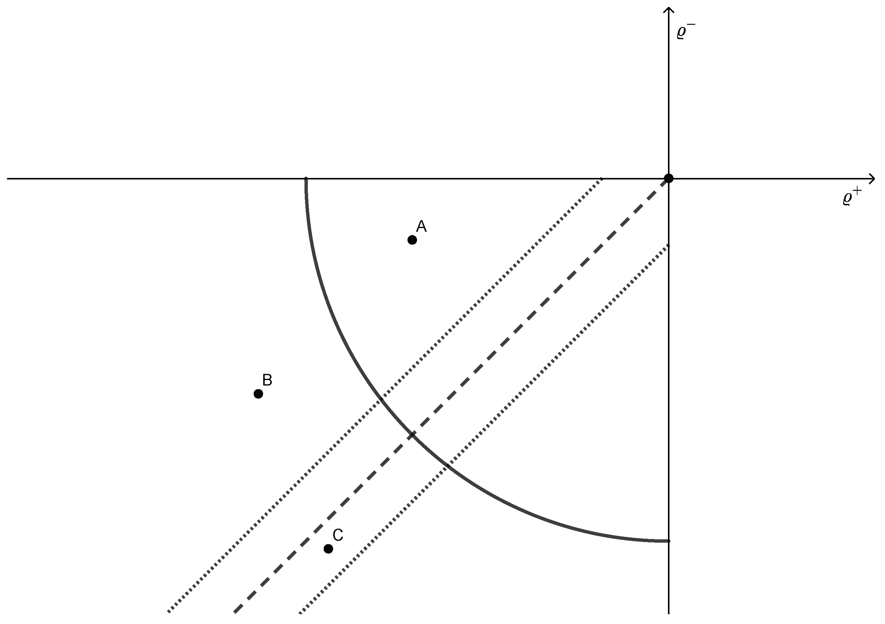
The difficulties to obtain the correct size of tests for asymmetry with cointegration pretesting can also be illustrated from a geometrical perspective. In general, the acceptance region for a joint hypothesis on uncorrelated coefficients ${\varrho }^{+}$ and ${\varrho }^{-}$ is an ellipse, its axes parallel to the coordinate axis with the length from end to end along one axis being $d_1=2se\left({\widehat{\varrho }}_1\right)Q_F(1-\alpha )$ and its length along the other axis being $d_2=2se\left({\widehat{\varrho }}_2\right)Q_F(1-\alpha )$, where $Q_F(·)$ denotes the quantile function of $F_{CI}$ and the origin corresponds to the null hypothesis (here: ${\varrho }^{+}={\varrho }^{-}=0$). In this particular model, we can assume without loss of generality that the standard errors of ${\varrho }^{+}$ and ${\varrho }^{-}$ have the same magnitude. Hence, the ellipse becomes a circle with radius $r=\frac{d_1}{2}=\frac{d_2}{2}$.

Figure 1 displays a sketch of the acceptance region in the Cartesian plane. The null hypothesis of no cointegration is not rejected if one of the coefficients is positive so that we restrict the analysis to the third quadrant of the plane. Moving to a higher level of confidence shifts the circle further away from the origin. The null hypothesis of symmetric adjustment is represented by the dashed bisector and its acceptance region is indicated by two dotted lines. The composite rejection region is located to the left of the circle and outside of both dotted lines. We have added three points in the plane to illustrate the properties of the composite test. Point A coincides with a coefficient combination which should not lead to a rejection of symmetric adjustment. Point B lies within the acceptance region of the cointegration test. Although the combination of ${\varrho }^{+}$ and ${\varrho }^{-}$ is asymmetric, we cannot reject the null hypothesis of no cointegration and the test for equality of coefficients is not conducted. If we maintain the same ratio of ${\varrho }^{+}$ and ${\varrho }^{-}$ and move to Point C, the $F_{CI}$ statistic would increase and the null hypothesis of symmetric adjustment would be rejected. While it is more difficult to reject the null hypothesis of symmetric adjustment for combinations close to the origin considering the width of the acceptance region relative to the area of all possible combinations of ${\varrho }^{+}$ and ${\varrho }^{-}$, it is much easier to reject far from the origin. If we compare the composite test to the unconditional test for asymmetry, the latter does not specifically take the exclusion of the cointegration test acceptance region into account, where the null hypothesis is hardly ever rejected although the coefficients differ. Consequently, using critical values obtained from the standard F-distribution leads to size distortions.

In order to improve the ability of the cointegration test to detect cointegration, Enders and Siklos (2001) suggest to follow Chan (1993) and select the threshold $\tau$ by optimizing the SSE of regression (3). In practice, this is achieved by estimating many regressions with fixed $\tau$, where $\tau$ runs through to all values of the cointegration residual series (SETAR) or its first difference (MTAR). Chan (1993) has shown that this procedure results in a superconsistent estimator for the threshold value which we denote by ${\tau }^{*}$. Usually a 100q percentage lateral trimming is applied to avoid ${\tau }^{*}$ becoming too close to the extreme values and hence ensuring a sufficient number of observations in each regime. This procedure, however, has important implications for the follow-up tests for asymmetry as the threshold parameter is not identified under the null hypothesis. Considering a specification with no additional lags, the F-statistic takes the form of

$$F_{apt}\left(\tau \right)=\frac{(SS{E}_1-SS{E}_2\left(\tau \right))}{SS{E}_2\left(\tau \right)}(n-p_2),$$

(13)

where $SS{E}_1$ denotes the sum of squared errors for the symmetric model (${\varrho }^{+}={\varrho }^{-}$), $SS{E}_2\left(\tau \right)$ denotes the sum of squared errors for the asymmetric model depending on the threshold parameter $\tau$ and $p_2$ denotes the number of parameters in the asymmetric model (here $p_2=2$). Therefore, we observe that the F-statistic is a function of the nuisance parameter $\tau$. Since $SS{E}_1$ is fixed, it holds that $F\left(\tau \right)\uparrow$ for $SS{E}_2\left(\tau \right)\downarrow$. Optimizing the threshold value with respect to the SSE criterion leads to generally oversized tests for asymmetry if we assume the incorrect standard F-distribution in those cases Hansen (1996, 1999).

One way to obtain correctly sized tests is to bootstrap the distribution of the F-statistics. We employ a residual bootstrap algorithm similar to the procedure described in Hansen (1996) for SETAR processes or in Caner and Hansen (2001) for MTAR processes with a potential unit root. The algorithm is designed as follows:

(1)

Estimate the long-run equilibrium equation to obtain ${\widehat{\beta }}_0$, ${\widehat{\beta }}_1$ and the cointegration residuals ${\widehat{z}}_t$. Conduct the F-test for asymmetry based on the MTAR/SETAR model and save $F_{apt}$.

(2)

Estimate the symmetric model

$$\Delta z_t=\varrho z_{t-1}+\sum _{j=1}^k{\gamma }_j\Delta z_{t-j}{\epsilon }_t$$

to obtain $\widehat{\varrho }$, ${\widehat{\gamma }}_1,\dots ,{\widehat{\gamma }}_k$ and save the residuals ${\widehat{\epsilon }}_t$.

(3)

Draw randomly from the residuals ${\widehat{\epsilon }}_t$ to obtain a bootstrap sample ${\epsilon }_t^b$.

(4)

Generate the bootstrap cointegration residuals series as $\Delta z_t^b=\widehat{\varrho }{z}_{t-1}^b+{\sum }_{j=1}^k{\widehat{\gamma }}_j\Delta z_{t-j}^b+{\epsilon }_t^b$ and use $(z_1^b,\dots ,z_k^b)=({\widehat{z}}_1,\dots ,{\widehat{z}}_k)$ as initial observations.

(5)

Generate the bootstrap variable $y_t^b={\widehat{\beta }}_0+{\widehat{\beta }}_1{x}_t+z_t^b$.

(6)

Estimate the long-run equilibrium equation for $y_t^b$ and $x_t$ and re-estimate the MTAR/SETAR model to compute the bootstrap F-statistic, $F_{apt}^b$.

(7)

Repeat (2) to (6) sufficiently often to obtain the empirical distribution of $F_{apt}^b$. Compute the p-value for $F_{apt}$ based on the bootstrap distribution.

The performance of bootstrapped tests for asymmetry is evaluated in the following section.

3. Simulations

In order to investigate the empirical size of test for asymmetry in fixed threshold and optimizing threshold models, we simulate a large number of symmetrically cointegrated time series $x_t$ and $y_t$ and report the probability that the test, performed at the 5%-level, falsely detects asymmetry. The data-generating process is given by

$$\begin{array}{ccc}\hfill y_t& =& {\beta }_0+{\beta }_1{x}_t+z_t,\hfill \\ \hfill \Delta x_t& =& {\xi }_t,\hfill \\ \hfill \Delta z_t& =& \varrho z_{t-1}+{\epsilon }_t,{\xi }_t,{\epsilon }_t\sim N(0,{\sigma }^2),\hfill \end{array}$$

(14)

where ${\beta }_0=0$, ${\beta }_1=1$ and ${\sigma }^2=1$. Note that we thereby completely conform to the modelling framework of Enders and Siklos (2001): No misspecification of the long-run equilibrium equation and having normally distributed iid error terms which are in particular not serially correlated as the number of lags $\Delta z_{t-j}$ is known in advance.4

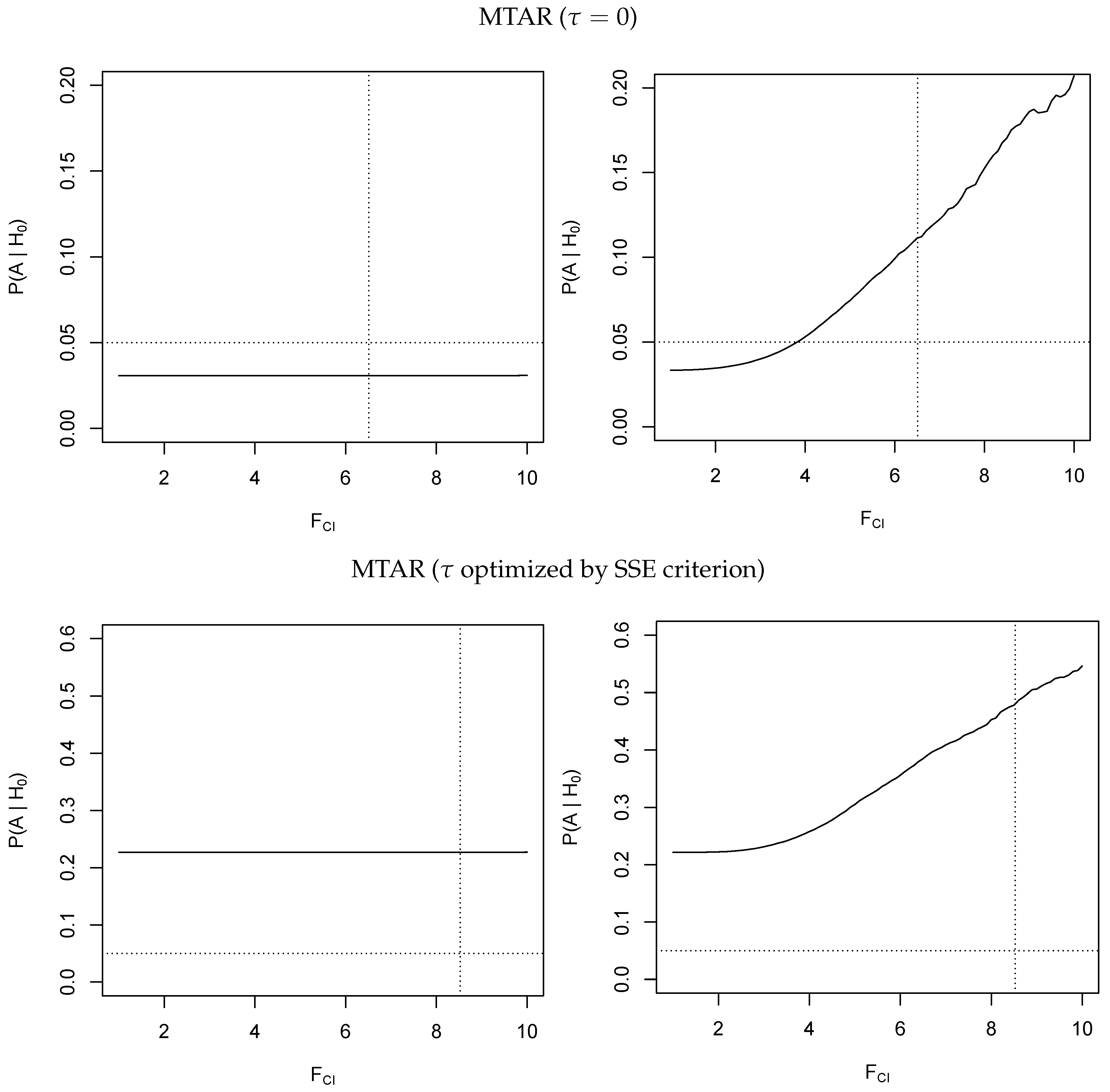
We first estimate an MTAR model with a known threshold of $\tau =0$ and display the rejection rates as a function of the statistic $F_{CI}$ obtained from the primary cointegration test. The results are plotted in the upper panel of Figure 2. The rejection rates are calculated from 20,000 replications using a sample size of $T=100$. We observe that the test is severely oversized for $\varrho =-0.1$ and the extent of oversizing increases with the value of the estimated F-statistic of the primary cointegration test (solid line in Figure 2). This means that in those empirical applications with small samples where a cointegration relationship is confirmed, we automatically tend to report asymmetric adjustment rates. It is not surprising that a test which is performed conditional on the outcome of a primary test does not match its nominal level of significance. The striking point here is that the mismatch is always in favor of falsely detecting asymmetry and that this discrepancy seems to be inversely related to the p-value of the cointegration test. In contrast, we do not report any size distortions which depend on the primary cointegration test for moderate adjustment coefficients ($\varrho <-0.5$) where the power of the cointegration test is close to unity. In those cases, the empirical size is slightly below the nominal size of 5%. Further simulations, which are not reported, show that the size distortions vanish if the sample size increases, providing further evidence that these size distortions are inversely related to the power of the primary cointegration test. As expected from our theoretical derivations, we do not find any size distortions if the power of the cointegration test reaches unity.

Repeating our simulations for optimizing threshold values using a 15% lateral trimming yields very different results which are displayed in the lower panel of Figure 2. Although we still notice oversizing from requiring evidence for cointegration, we find that the test for asymmetry in the MTAR model with optimizing threshold values is already substantially oversized for moderate adjustment coefficients. Since the threshold is not identified when adjustment is symmetric, the conditional least squares procedure seems to falsely select threshold values which artificially generate asymmetric adjustment estimates and result in a substantial difference in the sum of squared errors between the symmetric and asymmetric specification (see Equation (13)). Moreover, as reported in

Table 1. Empirical size of tests for asymmetry using estimated threshold values.

MTAR		T		SETAR		T
$\mathit{q}$	100	200	400	$\mathit{q}$	100	200	400
0.25	0.162	0.185	0.200	0.25	0.022	0.022	0.027
0.20	0.192	0.218	0.20	0.042	0.044	0.052
0.15	0.227	0.257	0.277	0.15	0.073	0.081	0.090
0.10	0.260	0.303	0.327	0.10	0.121	0.135	0.148
0.05	0.312	0.361	0.401	0.05	0.196	0.223	0.240

Note: The nominal level of significance is 5%. The lateral trimming parameter q denotes the percentage of observations which are deleted from the upper and lower end of the set of possible threshold values.

, the extent of oversizing increases with the sample size and cannot be sufficiently controlled by extensive lateral trimming.

We now turn to the SETAR models. The results with known threshold $\tau =0$, displayed in the upper panel of Figure 3, are surprisingly different from the fixed threshold MTAR results. The empirical size is close to zero across a wide range of adjustment coefficients which makes it difficult to assess the dependence on the primary cointegration test. However, taking the generally low power of the test for asymmetry in SETAR models into account, we still observe the effect of the power curve inflation factor. This result can also be related to prior studies reporting an underrejection of the null hypothesis (see, for example, Cook et al. (1999) and Galeotti et al. (2003)). Conversely, the test for asymmetry in SETAR models using optimizing threshold values, displayed in the lower panel of Figure 3, shows a behavior similar to the MTAR model. In this case, it is possible, however not recommended, to control the size of the test by moving to a stronger lateral trimming (see Table 1).

Finally, we analyze the empirical size and power of the proposed bootstrap tests for different combinations of ${\varrho }^{+}$ and ${\varrho }^{-}$. A Monte Carlo simulation experiment concerned with bootstrap procedures has to fulfil $B,R\to \infty$, where R is the number of replications and B is the number of bootstrap draws. Assuming that the number of bootstrap replications is fixed, every added Monte Carlo iteration contributes multiplicatively to the overall computational cost. To avoid this inefficiency, we refer to the ‘Warp-speed’ bootstrap described in Giacomini et al. (2013). The authors provide a formal proof that it is sufficient to draw only one bootstrap replication in each Monte Carlo replication and to evaluate the statistic of interest against the resulting bootstrap distribution of size R. The results for fixed and optimizing threshold values are displayed in

Table 2. Size and power of bootstrap tests for asymmetry.

$\mathit{\varrho }=-0.5$	MTAR			SETAR
T	100	200	400	100	200	400
$\alpha$ = 10%	0.103	0.101	0.102	0.109	0.105	0.100
5%	0.053	0.053	0.052	0.058	0.052	0.053
1%	0.010	0.011	0.010	0.012	0.009	0.012
${\mathit{\varrho }}^{+}=-\mathbf{0.75},{\mathit{\varrho }}^{-}=-\mathbf{0.5},\mathit{\tau }=\mathbf{0}$
T	100	200	400	100	200	400
$\alpha$ = 10%	0.254	0.403	0.638	0.226	0.370	0.619
5%	0.162	0.288	0.513	0.143	0.254	0.502
1%	0.059	0.129	0.284	0.045	0.095	0.259
${\mathit{\varrho }}^{+}=-\mathbf{0.75},{\mathit{\varrho }}^{-}=-\mathbf{0.25},\mathit{\tau }=\mathbf{0}$
T	100	200	400	100	200	400
$\alpha$ = 10%	0.553	0.821	0.977	0.456	0.752	0.962
5%	0.424	0.725	0.954	0.339	0.640	0.929
1%	0.215	0.503	0.860	0.151	0.394	0.810

Note: We use $20,000$ replications of the DGP for each combination of ${\varrho }^{+}$ and ${\varrho }^{-}$ and apply the ‘Warp-speed’ bootstrap algorithm described in Giacomini et al. (2013). The nominal significance level is denoted by $\alpha$.

and

Table 3. Size and power of bootstrap tests for asymmetry (SSE optimization).

$\mathit{\varrho }=-0.5$	MTAR			SETAR
T	100	200	400	100	200	400
$\alpha$ = 10%	0.082	0.091	0.090	0.109	0.101	0.101
5%	0.038	0.047	0.042	0.055	0.051	0.052
1%	0.007	0.010	0.008	0.010	0.010	0.011
${\mathit{\varrho }}^{+}=-\mathbf{0.75},{\mathit{\varrho }}^{-}=-\mathbf{0.5},\mathit{\tau }=\mathbf{0}$
T	100	200	400	100	200	400
$\alpha$ = 10%	0.232	0.446	0.748	0.198	0.300	0.500
5%	0.144	0.327	0.640	0.119	0.197	0.375
1%	0.042	0.145	0.410	0.034	0.067	0.183
${\mathit{\varrho }}^{+}=-\mathbf{0.75},{\mathit{\varrho }}^{-}=-\mathbf{0.25},\mathit{\tau }=\mathbf{0}$
T	100	200	400	100	200	400
$\alpha$ = 10%	0.595	0.896	0.996	0.440	0.730	0.954
5%	0.466	0.833	0.992	0.322	0.607	0.914
1%	0.241	0.643	0.961	0.133	0.361	0.780

Note: We use $20,000$ replications of the DGP for each combination of ${\varrho }^{+}$ and ${\varrho }^{-}$ and apply the ‘Warp-speed’ bootstrap algorithm described in Giacomini et al. (2013). The threshold values are determined from the conditional least squares procedure (Chan 1993). The nominal significance level is denoted by $\alpha$.

. We observe that the bootstrap F-tests maintain approximately the correct size and show suitable power properties for fixed threshold values and optimizing threshold values using a 15% lateral trimming. However, we still find size distortions originating from the hierarchical testing principle (not reported).

4. Application: (A)symmetric Fuel Price Transmissions

In the following, we investigate the potentially asymmetric price transmission from crude oil prices to retail gasoline prices in the US, Canada, France, Great Britain, Germany and Italy. We apply the threshold cointegration model to the data and test for asymmetry using conventional and bootstrapped critical values. Our weekly data cover the period from January 2010 until September 2017. WTI is the lead crude oil benchmark price for the North American market and Brent takes that role for the European market. Both crude oil price series and gasoline prices excluding tax and duty are obtained from Thomson Reuters Datastream. The Canadian prices are obtained from the Kent Group database. Using 405 observations and assuming moderate speed of adjustment, the power of the residual-based cointegration test is approximately unity, hence the first effect described in this paper (inflating the level of significance by conditioning on the primary cointegration test) should not play a role.

The results for MTAR and SETAR specifications are reported in

Table 4. Fuel price transmission.

Panel (a): MTAR ($\mathit{\tau }=0$)
	${\mathit{\varrho }}^{+}$	${\mathit{\varrho }}^{-}$	${\mathit{F}}_{\mathit{CI}}$	${\mathit{F}}_{\mathit{apt}}$	$\mathit{p}$-Value
US	$-0.069$	$-0.075$	$8.450$ ***	0.022	0.882 (0.428)
CAN	$-0.052$	$-0.105$	$8.453$ ***	1.822	0.178 (0.162)
FRA	$-0.191$	$-0.205$	$23.880$ ***	0.059	0.808 (0.793)
GBR	$-0.197$	$-0.112$	$18.360$ ***	2.599	0.108 (0.092)
GER	$-0.120$	$-0.165$	$13.730$ ***	0.691	0.406 (0.363)
ITA	$-0.234$	$-0.167$	$23.300$ ***	1.277	0.259 (0.242)
Panel (b): SETAR ($\mathit{\tau }=\mathbf{0}$)
	${\mathit{\varrho }}^{+}$	${\mathit{\varrho }}^{-}$	${\mathit{F}}_{\mathit{CI}}$	${\mathit{F}}_{\mathit{apt}}$	$\mathit{p}$-Value
US	$-0.081$	$-0.058$	$8.949$ ***	0.455	0.500 (0.252)
CAN	$-0.090$	$-0.062$	$7.794$ **	0.519	0.472 (0.220)
FRA	$-0.190$	$-0.208$	$23.910$ ***	0.097	0.756 (0.612)
GBR	$-0.170$	$-0.133$	$17.220$ ***	0.486	0.486 (0.278)
GER	$-0.125$	$-0.159$	$13.580$ ***	0.385	0.535 (0.285)
ITA	$-0.195$	$-0.211$	$22.650$ ***	0.070	0.792 (0.663)
Panel (c): MTAR (τ *)
	${\mathit{\varrho }}^{+}$	${\mathit{\varrho }}^{-}$	${\mathit{F}}_{\mathit{CI}}$	${\mathit{F}}_{\mathit{apt}}$	$\mathit{p}$-Value
US	$-0.113$	$-0.057$	$9.587$ ***	1.847	0.175 (0.735)
CAN	$-0.047$	$-0.144$	$10.160$ ***	5.333	0.021 (0.172)
FRA	$-0.318$	$-0.171$	$25.370$ ***	4.361	0.037 (0.195)
GBR	$-0.326$	$-0.111$	$22.840$ ***	11.750	0.001 (0.013)
GER	$-0.106$	$-0.191$	$14.180$ ***	2.460	0.118 (0.532)
ITA	$-0.338$	$-0.163$	$25.220$ ***	6.405	0.012 (0.097)
Panel (d): SETAR (τ *)
	${\mathit{\varrho }}^{+}$	${\mathit{\varrho }}^{-}$	${\mathit{F}}_{\mathit{CI}}$	${\mathit{F}}_{\mathit{apt}}$	$\mathit{p}$-Value
US	$-0.106$	$-0.037$	$10.750$ ***	4.074	0.044 (0.092)
CAN	$-0.111$	$-0.052$	$8.596$ **	2.311	0.129 (0.247)
FRA	$-0.176$	$-0.240$	$23.610$ ***	1.209	0.272 (0.540)
GBR	$-0.178$	$-0.123$	$17.060$ ***	1.070	0.302 (0.588)
GER	$-0.109$	$-0.194$	$14.120$ ***	2.355	0.126 (0.230)
ITA	$-0.187$	$-0.228$	$21.930$ ***	0.462	0.497 (0.862)

Note: One additional lagged difference was included in the threshold regressions to accommodate the dynamic structure of the cointegration residuals. The lag order was chosen based on the BIC and additional residual diagnostics. $F_{CI}$ denotes the F-statistic for the null hypothesis ${\varrho }^{+}={\varrho }^{-}=0$. Critical values are tabulated in Enders and Siklos (2001). $F_{apt}$ denotes the F-statistic for the null hypothesis ${\varrho }^{+}={\varrho }^{-}$. The last column reports the p-value for the test for asymmetry using a standard F-distribution while the p-value from the bootstrap test is given in parentheses. *** $p<0.01$, ** $p<0.05$, * $p<0.1$.

. All crude oil and retail gasoline price pairs are cointegrated. We compare the results for the conventional test for long-run asymmetry against the results for the bootstrap test described in Section 2. In general, the p-value for conventional F-tests are higher than the ones obtained from bootstrapping for the fixed threshold models and lower for the models using optimizing threshold values. This is not surprising, considering that our simulation experiments have shown that conventional tests for long-run asymmetry are undersized for fixed thresholds and oversized for optimizing threshold values. If we use bootstrap-corrected p-values, we only find evidence for asymmetric adjustment at the 5% significance level in case of the Great Britain retail gasoline market (MTAR model with optimal threshold value). For the US retail gasoline market and SETAR specification, we would reject the null hypothesis of symmetric adjustment for conventional F-tests but would not do so using our bootstrap algorithm. The same holds for Canada, France and Italy if we employ an MTAR model with optimal threshold values.

5. Summary and Concluding Remarks

It was shown in this paper that the test for long-run asymmetry in residual-based threshold cointegration models is confounded towards indicating asymmetry by preconditioning the test on finding sufficient evidence for cointegration. The extent of oversizing the test depends inversely on the power of the primary cointegration test. For purposes of demonstration, we selected scenarios with substantial size distortions, which are characterized by a small sample size and relatively small adjustment coefficients. Additionally, our simulation experiments show that tests for asymmetry based on standard F-distributions are generally oversized if the threshold value is estimated by conditional least squares.

Our results help to understand why contradictory statements on the performance of tests for asymmetry persist in the literature. On one hand, these tests are reported to have a tendency to underreject the hypothesis of symmetry which is related to the fact that they are undersized for fixed thresholds and moderate to large samples. On the other hand, we can explain why studies on asymmetric pricing appear to be more likely to find evidence for asymmetry if they employ error correction models which require evidence for a cointegration relationship (see Perdiguero-Garcia (2013) for a meta-analysis on asymmetric price transmission in gasoline markets) and/or use optimizing threshold values.

Similar size distortions might not be specific to the Enders-Siklos procedure alone, but might also be latent in other methods where cointegration tests and tests for asymmetry are conducted on the same parameter space. Particularly, tests for asymmetry in the context of smooth transition autoregressive (STAR) models (Teräsvirta 1994; Van Dijk et al. 2002) or buffered autoregressive models (Li et al. 2015; Zhu et al. 2017) might be affected in the same way if they were applied to cointegration residuals. We recommend that practitioners use bootstrap tests for asymmetry similar to the one outlined in this paper instead of conventional F-tests. Further, we recommend to choose a conservative level of significance when conducting tests for asymmetry in momentum threshold cointegration models using fixed thresholds and small samples.

References

- Caner, Mehmet, and Bruce E. Hansen. 2001. Threshold Autoregression with a Unit Root. Econometrica 69: 1555–96. [Google Scholar] [CrossRef]
- Chan, Kung-Sik. 1993. Consistency and Limiting Distribution of the Least Squares Estimator of a Threshold Autoregressive Model. The Annals of Statistics 21: 520–33. [Google Scholar] [CrossRef]
- Cook, Steven, Sean Holly, and Paul Turner. 1999. The power of tests for non-linearity: The case of Granger-Lee asymmetry. Economics Letters 62: 155–59. [Google Scholar] [CrossRef]
- Enders, Walter, and Clive W. J. Granger. 1998. Unit-Root Tests and Asymmetric Adjustment with an Example using the Term Structure of Interest Rates. Journal of Business & Economic Statistics 16: 304–11. [Google Scholar] [CrossRef]
- Enders, Walter, and Pierre L. Siklos. 2001. Cointegration and Threshold Adjustment. Journal of Business & Economic Statistics 19: 166–76. [Google Scholar] [CrossRef]
- Engle, Robert F., and Clive W. J. Granger. 1987. Co-Integration and Error Correction: Representation, Estimation and Testing. Econometrica 55: 251–76. [Google Scholar] [CrossRef]
- Frey, Giliola, and Matteo Manera. 2007. Econometric Models of Asymmetric Price Transmission. Journal of Economic Surveys 21: 349–415. [Google Scholar] [CrossRef]
- Galeotti, Marzio, Alessandro Lanza, and Matteo Manera. 2003. Rockets and feathers revisited: An international comparison on European gasoline markets. Energy Economics 25: 175–90. [Google Scholar] [CrossRef]
- Giacomini, Raffaella, Dimitris N. Politis, and Halbert White. 2013. A Warp-Speed Method for Conducting Monte Carlo Experiments Involving Bootstrap Estimators. Econometric Theory 29: 567–89. [Google Scholar] [CrossRef]
- Godby, Rob, Anastasia M. Lintner, Thanasis Stengos, and Bo Wandschneider. 2000. Testing for asymmetric pricing in the Canadian retail gasoline market. Energy Economics 22: 349–68. [Google Scholar] [CrossRef]
- Grasso, Margherita, and Matteo Manera. 2007. Asymmetric error correction models for the oil-gasoline price relationship. Energy Policy 35: 156–77. [Google Scholar] [CrossRef]
- Hansen, Bruce E. 1996. Inference when a Nuisance Parameter is not identified under the Null Hypothesis. Econometrica 64: 413–30. [Google Scholar] [CrossRef]
- Hansen, Bruce E. 1999. Testing for linearity. Journal of Economic Surveys 13: 551–76. [Google Scholar] [CrossRef]
- Honarvar, Afshin. 2010. Modeling of Asymmetry between Gasoline and Crude Oil Prices: A Monte Carlo Comparison. Computational Economics 36: 237–62. [Google Scholar] [CrossRef]
- Karoglou, Michail, and Bruce Morley. 2012. Purchasing power parity and structural instability in the US/UK exchange rate. Journal of International Financial Markets, Institutions and Money 22: 958–72. [Google Scholar] [CrossRef]
- Lee, Oesook, and Dong Wan Shin. 2000. On geometric ergodicity of the MTAR process. Statistics & Probability Letters 48: 229–37. [Google Scholar] [CrossRef]
- Li, Guodong, Bo Guan, Wai Keung Li, and Philip L. H. Yu. 2015. Hysteretic autoregressive time series models. Biometrika 102: 717–23. [Google Scholar] [CrossRef]
- Mohammadi, Hassan. 2011. Market integration and price transmission in the U.S. natural gas market: From the wellhead to end use markets. Energy Economics 33: 227–35. [Google Scholar] [CrossRef]
- Norman, Stephen. 2008. Systematic small sample bias in two regime SETAR model estimation. Economics Letters 99: 134–38. [Google Scholar] [CrossRef]
- Payne, James E., and George A. Waters. 2008. Interest rate pass through and asymmetric adjustment: Evidence from the federal funds rate operating target period. Applied Economics 40: 1355–62. [Google Scholar] [CrossRef]
- Perdiguero-Garcia, Jordi. 2013. Symmetric or asymmetric oil prices? A meta-analysis approach. Energy Policy 57: 389–97. [Google Scholar] [CrossRef]
- Petruccelli, Joseph D., and Samuel W. Woolford. 1984. A Threshold AR(1) Model. Journal of Applied Probability 21: 270–86. [Google Scholar] [CrossRef]
- Simioni, Michel, Frédéric Gonzales, Patrice Guillotreau, and Laurent Le Grel. 2013. Detecting Asymmetric Price Transmission with Consistent Threshold along the Fish Supply Chain. Canadian Journal of Agricultural Economics 61: 37–60. [Google Scholar] [CrossRef]
- Teräsvirta, Timo. 1994. Specification, Estimation, and Evaluation of Smooth Transition Autoregressive Models. Journal of the American Statistical Association 89: 208–18. [Google Scholar] [CrossRef]
- Thompson, Mark A. 2006. Asymmetric adjustment in the prime lending-deposit rate spread. Review of Financial Economics 15: 323–29. [Google Scholar] [CrossRef]
- Tong, Howell. 1978. On a Threshold Model, Pattern Recognition, and Signal Processing. Amsterdam: Sijthoff and Noordhoff. [Google Scholar]
- Van Dijk, Dick, Timo Teräsvirta, and Philip Hans Franses. 2002. Smooth Transition Autoregressive Models—A Survey of Recent Developments. Econometric Reviews 21: 1–47. [Google Scholar] [CrossRef]
- Von Cramon-Taubadel, Stephan, and Jochen Meyer. 2000. Asymmetric Price Transmission: Fact of Artefact? Working Paper. Göttingen, Germany: University of Göttingen, pp. 1–22. [Google Scholar]
- Zhu, Ke, Wai Keung Li, and Philip L. H. Yu. 2017. Buffered Autoregressive Models with Conditional Heteroscedasticity: An Application to Exchange Rates. Journal of Business and Economic Statistics 35: 528–42. [Google Scholar] [CrossRef]