Structural Panel Bayesian VAR Model to Deal with Model Misspecification and Unobserved Heterogeneity Problems


Department of Political Sciences, LUISS Guido Carli University and CEFOP-LUISS, 00197 Rome, Italy
Econometrics 2019, 7(1), 8; https://0-doi-org.brum.beds.ac.uk/10.3390/econometrics7010008
Submission received: 4 September 2018
/
Revised: 23 February 2019
/
Accepted: 5 March 2019
/
Published: 11 March 2019
(This article belongs to the Special Issue Big Data in Economics and Finance)
Abstract
:This paper provides an overview of a time-varying Structural Panel Bayesian Vector Autoregression model that deals with model misspecification and unobserved heterogeneity problems in applied macroeconomic analyses when studying time-varying relationships and dynamic interdependencies among countries and variables. I discuss what its distinctive features are, what it is used for, and how it can be analytically derived. I also describe how it is estimated and how structural spillovers and shock identification are performed. The model is empirically applied to a set of developed European economies to illustrate the functioning and the ability of the model. The paper also discusses more recent studies that have used multivariate dynamic macro-panels to evaluate idiosyncratic business cycles, policy-making, and spillover effects among different sectors and countries.
Keywords:
panel VAR; Bayesian inference; structural spillovers; hierarchical priors; MCMC implementationsJEL Classification:
13/A2; 13/A4; 13/A5; 13/D1; 13/D21. Introduction
Macroeconomic analyses and policy evaluations have given new momentum to the study of business cycles and policy-making, and consideration of interdependencies and co-movements among different sectors and countries is a modern requirement. Even economic–institutional issues, often not directly observed, and the transmission of certain shocks, often idiosyncratic, now need to be evaluated from a global perspective and in a unified framework for either large or developed economies (see, e.g., Canova and Ciccarelli (2009); Canova et al. (2012); Sims and Zha (1998), and Ciccarelli and Rebucci (2007); Ciccarelli et al. (2018)). Thus, when formulating policies or forecasting, several issues need to be considered, such as the reasons underlying the different reactions among countries, the causality between real and financial variables, the additional transmission channels that allow shocks to spill over, and the economic and institutional implications of driving shock transmission. However, although estimation of time-varying structures is feasible with a large homogeneous cross-section, heterogeneous dynamics due to an unexpected shock combined with economic–institutional interdependencies makes it difficult to exploit cross-sectional information to estimate time series variations in multicountry setups.
The model suggested in this paper is based on a time-varying Structural Panel Bayesian Vector Autoregression (SPBVAR) model and aims to deal with model misspecification and unobserved heterogeneity problems when jointly modeling and quantifying multicountry data using the information contained in a large set of endogenous and economic–institutional variables. I define a hierarchical prior specification strategy (see, e.g., Koop (1996); Canova and Ciccarelli (2004, 2009), and Ciccarelli et al. (2018)) and Markov Chain Monte Carlo (MCMC) implementations (see, e.g., Chib (1995, 1996); Albert and Chib (1993); Chib and Jeliazkov (2001); Pesaran and Shinb (1998), and Carter and Kohn (1994)) to calculate posterior distributions of Conditional Generalized Impulse Response Functions (CGIRFs) and Conditional Forecasts (CF) reacting to unexpected perturbations in the innovations of factors in the system. Bayesian methods are used to reduce the dimensionality of the model, structure the time variations, and evaluate issues of endogeneity. I further build on Ciccarelli et al. (2018) and use a Structural Normal Linear Regression (SNLR) model to work with smaller systems in which the regressors are observable, directly measured, and time-varying linear combinations of the right-hand variables of the time-varying SPBVAR. The advantage of this approach is that it is easier to match endogenous variables to additional time-variant factors. Here, the framework is valid if and only if prior specifications are satisfied and a fully hierarchical structure is provided. Thus, an analysis of joint and conditional densities and sequential factorization are required.
In this paper, the time-varying SPBVAR model incorporates the econometric literature on multicountry (dynamic) panel data models for applied macroeconomic financial analysis. In recent years, several theoretical and applied models have been developed to infer and evaluate idiosyncratic shocks across units and time periods by accounting for several additional transmitted shocks and additional spillover effects (see, e.g., Lane and Milesi-Ferretti (2007); Mastrogiacomo et al. (2017); Facchini et al. (2017); Degiannakis et al. (2016); Crespo-Cuaresma and Fernandez-Amadorb (2013); Canova and Marrinan (1997); Reinhart and Rogoff (2009), and Ciccarelli and Rebucci (2007)). These studies have generated three main findings. First, there are institutional and economic interdependencies among countries, especially among Eurozone countries, which have relinquished independent monetary and exchange rate policies. Second, there may still be a substantial degree of heterogeneity, with some common behaviors, in economic–financial linkages among countries, and those linkages may have changed over time due to different transmission channels. Third, there is a need to allow for cross-country and cross-variable interdependencies when studying real and financial linkages. Nevertheless, such studies have reached very different conclusions and neglected some of these problems, rendering functional form misspecification and heterogeneity issues topics that need to be implemented with care. These discrepancies and deficiencies may exist because of diverging methodologies when assuming structural relationships or lagged interdependencies among factors, as well as alternative approaches to assessing cross-country shock transmission and spillover effects (e.g., time-invariant factors, exogenous variables, restrictions on time periods to which time-varying coefficients can be added).
My approach and empirical application aim to contribute to this debate. More precisely, they build on Ciccarelli et al. (2018), who investigated heterogeneity and spillovers in macro-financial linkages among developed economies, focusing on the most recent recession. They developed a time-varying panel Bayesian VAR model including real and financial variables and identified a statistically significant common component. Nevertheless, their empirical model is non-structural and constrained because of time-invariant or exogenous factors in the system, so it is unable to identify structural and institutional differences among countries, different reactions to a common unexpected shock, and the causality among real and financial variables.
The methodological implementation described in this paper consists of extending their model and thus their flexible factorization to add more time-varying endogenous factors to the system, and this change affects the variables of interest in different time periods. The idea is that shock transmission and economic–institutional linkages affect spillover effects among countries and variables over time and depend on a set of directly observed and hidden1 factors, respectively. By comparing these factors and allowing each country to load them, model misspecification and unobserved heterogeneity problems can be investigated. For example, I can assess how the dimension and intensification of spillovers over time affect commonality, interdependence, and heterogeneity among countries and variables; interdependencies in cross-country business cycles; how different transmission channels essentially affect the spread of spillovers in macroeconomic–financial linkages when given an unexpected shock; and the importance of economic and institutional implications in driving shock transmission.
The model described in this paper also relates to Giannone et al. (2009) and Koop (1996), who proposed large Bayesian VAR models to examine both the forecasting accuracy and structural analysis of the effect of a monetary policy shock by evaluating additional sectoral information and macroeconomic variables that were not used in the analysis by De Mol et al. (2008). In that study, shrinkage was obtained by using Minnesota priors, which are often uninformative since they are based on an approximation that involves replacing the variance–covariance matrix with an estimate. Moreover, the framework was extended by using a set of dummy variables that are invariant over time and thus difficult to model. My modeling and inference differ since I follow the hierarchical specification strategy of VAR and time-varying parameters.
Finally, an empirical application to a pool of developed European economies is described in this paper to illustrate the functioning and the ability of the model, with particular attention paid to the recent recession and post-crisis consolidation. There is a focus on three macroeconomic questions that are underdeveloped in the literature dealing with multicountry data. First, I examine how commonality, interdependence, and heterogeneity among countries and variables change over time as a result of an unexpected common shock. Second, I query how additional shock transmissions affect the spread and intensification of structural spillovers in the real and financial dimension. Third, I probe the extent to which economic–institutional linkages matter when studying co-movements and interdependencies among different countries and sectors.
The empirical analysis is robust and consistent with the more recent business cycle studies, which recognize the importance of (1) accounting for both group-specific and global factors when evaluating cross-country spillovers and (2) separating common shocks from the propagation of country- and variable-specific shocks when studying economic–financial linkages (see, e.g., Dees et al. (2007); Forni et al. (2000); Ciccarelli et al. (2018); Canova et al. (2007, 2012), and Beetsma and Giuliadori (2011)). The analysis does not include studies focused on regional cycles in Europe and on international transmission of shocks unless they contain interesting results from the viewpoint of the present paper. For example, Billio et al. (2016); Agudze et al. (2018), and Kaufmann (2010, 2015) addressed the question of whether international business cycles originate from common shocks or from a common propagation mechanism. More precisely, their findings focused on common movements of US regional business cycles and shock transmission between the US and Eurozone by evaluating possible interactions between a set of variables of interest. They built on Canova and Ciccarelli (2009) and extended their panel VAR model to model asymmetry and turning points in the business cycles of different countries and regions. They also built on the models of Krolzig (1997, 2000) and Sims and Zha (2006) by considering Markov-Switching dynamics to model covariance matrices of country-specific Markov chains, especially when transition probabilities differ among heterogeneous units. Moreover, to solve potential overfitting problems caused by the inclusion of many parameters in the model, the authors followed the same hierarchical prior specification strategy proposed in this paper and by Canova and Ciccarelli (2009). Finally, their empirical results met with positive feedback in my empirical analysis, highlighting the importance of specifying a coordinated economic policy within Eurozone economies and evidence of larger recessions in the Eurozone during the 1990s when the monetary union was planned.
Structural spillovers are evaluated through structural Bilateral Net Spillover Effects (BNSEs) and Systemic Contributions (SCs). The former incorporate feedback effects from the impulse variables and temporary or persistent long-run effects of a potential shock. The SC index represents the amplification contribution of an impulse variable to the response variable, and the index can capture sequential features associated with systemic events. Finally, the Generalized Theil (GT) index is estimated to investigate business cycle convergence and synchronization.
2. Econometric Model and Specifications
2.1. Model Estimation
The time-varying Structural Panel Bayesian VAR proposed in the paper has the following form:
where the subscripts are country indices, denotes time, L stands for the lag operator, is an vector of intercepts for each i, is an matrix of coefficients for each pair of countries for a given m, is an vector of lagged variables of interest for each i for a given m, is an matrix of coefficients for each pair of countries for a given q, is an vector including a set of lagged directly observed variables for each i for a given q, is an matrix of coefficients for each pair of countries for a given , is an vector including a set of lagged not directly observed variables for each i for a given , and is an vector of disturbance terms. The subscripts are lags for each of the endogenous variables, (directly) observed variables, and hidden variables. Here, all variables in the system are endogenous and time-varying.
In Equation (1), the dynamic relationships can be unit-specific, and all coefficients vary over time. In addition, whenever the matrices , , and differ2 for some L, cross-unit lagged interdependencies matter, and then dynamic feedback and interactions among countries and among variables are possible. Nevertheless, even if this feature adds flexibility to the specification, it is very costly. In fact, the number of coefficients is increased by factors.
Let be the number of all matrix coefficients in each equation of the SPBVAR model for each pair of countries . A vector can be defined, and it contains all lagged variables in the system for each i. Then, I define an vector containing all columns, stacked into a vector3, of the matrices , , and for each pair of countries for a given k, with , and denoting the time-varying coefficient vectors, stacked for i, for each country–variable pair. With these specifications, I can express the SPBVAR model in terms of a multivariate normal distribution:
where and are vectors containing the observable variables of interest and the random disturbances of the model for each i for a given m, respectively. Here, , and contains all T observations (stacked) for the first dependent variable, followed by all T observations for the second dependent variable, and so on. Moreover, there is no subscript i since all lagged variables in the system are stacked in .
Now, because the coefficient vectors in vary in different time periods for each country–variable pair and there are more coefficients than data points, it is impossible to eliminate . To solve this problem, I apply a flexible factorization for , proposed in Koop (1996), Canova and Ciccarelli (2009), and Ciccarelli et al. (2018), and extend it to estimate all coefficients and their possible interactions without restrictions or loss of efficiency:
where and by construction; are matrices obtained by multiplying the matrix coefficients () stacked in the vector by conformable matrices with elements equal to zero and one, where is a numerical index that depends on the typology of the factorization; is an vector of unmodeled variations present in , , where is the covariance matrix of the vector , and as in Kadiyala and Karlsson (1997). In the framework, unobserved heterogeneity and model specification are absorbed in the time-varying coefficient vectors . They are observable smooth linear functions of the lagged variables and can thus be easily estimated with a gain in efficiency.
The idea is to shrink to a much smaller dimensional vector , with , containing all regression coefficients stacked into a vector. In this way, further investigations (e.g., additional shock transmissions between different countries and sectors, additional spillover effects, and economic issues) can be performed. Finally, the factorization of becomes exact as long as converges to zero.
In Equation (3), all factors are permitted to be time-varying, and thus, time-variant structures can be obtained via implementations of MCMC algorithms. Moreover, time variations in the variance of shocks to the factors are also allowed so that can capture possible heterogeneity among countries and variables. Running Equations (2) and (3) for Equation (1), the factorization is:
The conformation of the SPBVAR model and the exact form of the ’s and the ’s are explained in Section 2.2.
The empirical implementation targets the potential addition of any and countless time-varying coefficient vectors to any time period, depending on the needs of the investigation. For example, according to the more recent studies of business cycles and spillover effects (see, e.g., Lane and Milesi-Ferretti (2007); Mastrogiacomo et al. (2017); Canova and Marrinan (1997); Reinhart and Rogoff (2009), and Ciccarelli and Rebucci (2007), among others), one tends to define a country-specific indicator, a cross-country variable-specific indicator, and a common indicator for . However, in this way, it makes it difficult to handle model misspecification and heterogeneity issues when dealing with multicountry data. Given the methodological approach pursued in this paper, running Equations (3) and (4) for the SPBVAR in Equation (1), one can deal with such issues. It represents the main thrust of this study, and it is expected to motivate the investigator to build up choices of additional factors for studying time-varying relationships and dynamic interdependencies among countries and variables in multicountry setups. For example, one may be interested in adding a set of lagged observable variables to the matrix to account for the role of transmission channels, which allow shocks to spill over, and a set of lagged proxy4 variables in the matrix to account for economic–institutional implications when identifying shock transmissions. An in-depth study is presented in Section 4.
Given the factorization in Equation (3), the reduced-form SPBVAR model in Equation (2) can be transformed into a SNLR model with an error covariance matrix of an Inverse–Wishart () distribution5. Its form would be similar to the parsimonious Seemingly Unrelated Regression (SUR) model developed in the literature (see, for instance, Canova and Ciccarelli (2009) and Ciccarelli et al. (2018)).
By Equations (2) and (3), the SNLR model can be written as
where contains all lagged time-varying variables in the system by construction, and is an matrix that stacks all coefficients of the system, with .
By construction, indices are linear combinations of right-hand variables of the system and correlated among each other. The vectors of M variables of interest, Q observable variables, and hidden factors depend on a small number of observable indices () and the factors that load the indices. Thus, the reparametrized SNLR model is simply a multivariate regression model.
When the factorization in (4) allows for an error, has a particular heteroskedastic covariance matrix that needs to be taken into account, with . If the factorization in Equation (4) is exact, , with , depends on the only disturbances contained in . Thus, it is uncorrelated with the regressors, and classical OLS can be used to estimate the vector and thus the vector . The correlation tends to decrease as k increases, and consistency is ensured as T grows.
The specification in Equation (5) implies that individual regressions are tied into a system of equations that can be analyzed together. In this context, when a Bayesian framework is applied, the posterior for the unknowns can be easily constructed. For example, given the assumptions of the error term , if the prior for is of the semi-conjugate type—, , , where are known quantities, W stands for Wishart distribution, and G denotes Gamma distribution6—one can use the Gibbs sampler construct sequences for from their joint posterior distribution. In the analysis, I use the reciprocal of the covariance matrix of the multivariate normal random vector , which allows Wishart and Gamma distributions to be used directly as a conjugate prior (see, for instance, Chib and Greenberg (1995a) and Pesaran et al. (2004)). Section 3 describes in detail the hierarchical prior strategy.
2.2. Model Features
To illustrate the conformation of the time-varying SPBVAR and the exact form of the ’s and the ’s in Equation (3), suppose there are endogenous variables and additional observable and hidden variables that vary over time for every countries. For convenience, I suppose one lag and no intercept. Thus, the SPBVAR in Equation (1) assumes the form:
Let be the vector containing all columns (stacked) of the matrices , , and for each pair of countries , with denoting the variables in each equation observed for j and independent of i, and let be the vector containing all lagged variables in the system for each i for a given k, with .
According to the more recent studies of business cycles and spillover effects (see, e.g., Ciccarelli et al. (2018); Canova et al. (2007, 2012); Billio et al. (2016); Agudze et al. (2018), and Kaufmann (2010, 2015)), it is typical for authors to define a country-specific indicator for for each i, a variable-specific indicator for for each m, and a common indicator for for each pair of countries and variables . However, in this study, the interest is in the identification of additional effects between different countries and sectors that vary over time and directly affect the variables of interest in . It represents the main thrust of this study and will drive the investigator to build up choices of the types of factors to avoid having mis-specified estimates due to unobserved heterogeneity when dealing with multicountry data.
In this example, I assess three additional terms in the factorization: an indicator to account for the role of additional transmission channels (e.g., in ) and the impact of economic interdependencies (e.g., in ) in driving the transmission of country-specific shocks; an indicator to investigate interdependence and commonality among all lagged variable that affect shock transmission; and an indicator to highlight different reactions and co-movements across countries and variables (, , ) due to an unexpected shock.
The factorization in Equation (3) becomes:
where is a vector capturing unaccounted features; is a vector containing all matrix coefficients, stacked in the vector , for each pair of countries for a given k; and, stacking for t, is a vector containing all time-varying coefficient vectors to be estimated. To be more precise: the factors and are mutually orthogonal vectors capturing movements in that are country-specific; the factor is an mutually orthogonal vector capturing movements in that are variable-specific, where denotes the number of variable groups; and the factor is an mutually orthogonal vector capturing movements in that are common among countries and among variables, where denotes the number of common groups. Letting , , , , , and , the conformable matrices in Equation (7) can be constructed in this way:
Thus, following some arrangements (as described in Section 2.1), the SNLR model in Equation (5) becomes:
Therefore, I obtain four matrices containing all coefficients (stacked) and their possible interactions in the SNLR model in Equation (Section 2.2). is an observable country-specific indicator for that captures the information contained in the lags of variable M for country 1 and country 2 , with and . is an observable country-specific indicator for that captures the information contained in a set of lagged variables for country 1 and country 2 , with and , with denoting all possible interactions between the lags of variables M, Q, and . is an observable cross-country variable-specific indicator for that captures, stacked for four groups (), the information contained in the lags of variable and variable . Here, and capture movements between the lags of the only variables M that are specific for variable and variable , respectively, and and capture movements between the lags of all variables M, Q, and that are specific for variable and variable , respectively. is an observable common indicator for that captures, stacked for two groups (), the information contained among countries and variable M () and among countries and variables M, Q, and (), with and .
3. Dynamic Analysis
3.1. Hierarchical Structure for Time-Varying Coefficient Vectors
Given the factorization in Equation (3), ’s are stochastic processes; thus, a specification of their law of motion is needed to complete the model. In this paper, I suppose the following state-space structure (see, for instance, Canova and Ciccarelli (2009)):
where ; is a block-diagonal matrix; and , where controls the tightness (stringent conditions) of the factorization (f) of the time-varying coefficient parameter () in order to make it estimable. The errors , , and are mutually independent.
In Equation (10), the factors driving the coefficients of the SPBVAR evolve over time as random walks. This specification is parsimonious since it concerns , which is of a much smaller dimension than that of and allows for the evaluation of coefficient changes that are permanent. Moreover, with the hierarchical strategy used to construct the SPBVAR, one would be able to investigate any type of coefficient factors via their interactions. The variance in can be time-variant. Such a specification implies Autoregressive Conditional Heteroskedasticity in Mean (ARCH-M) model effects in the representation of , and it is a way of modeling time-varying conditional second moments to provide an alternative to the stochastic volatility specification (see, e.g., Cogley and Sargent (2005)). The main difference is that volatility changes are replaced by coefficient changes. Moreover, the computational costs involved in using this specification are moderate since the dimension of is considerably smaller than the dimensionality of . Finally, the block diagonality of guarantees the identifiability of the factors ().
Given the assumptions of the error terms in Equations (3) and (5), the specification of Equations (3), (5), and (10) is estimable, and thus, prior assumptions can be specified, and Bayesian computations are feasible. Thus, the reparametrized SPBVAR model has a state-space structure:
Given the hierarchical structure, Bayesian estimation requires prior distributions for , , , and . These joint prior densities can be specified so that the posterior distribution for the quantities of interest can be computed numerically using MCMC methods (see, for instance, Canova and Ciccarelli (2009)). Finally, since the state-space structure in Equations (11) and (12) is linear, variations of the Kalman filter algorithm can be used to construct the likelihood function, which then can be maximized with respect to the relevant parameters (see, e.g., Litterman (1985)).
3.2. Prior Assumptions
Supposing exact factorization and letting be the prior densities, I assume two tentative beliefs (assumptions) for the model described in Equation (5). (i) Conditional Normality: ; it is a hierarchical prior for . (ii) Conditional Independence: .
A hierarchical prior for is already specified. Thus, to complete the model, the prior moments on need to be defined. The likelihood function can be derived from the sampling density , and it can be shown to be of a form that breaks into a mixture of distributions. In other words, (i) a normal distribution for factors ; (ii) a Wishart distribution for ; (iii) an Inverse-Gamma distribution for , where . That is,
where is the OLS estimate of ; is the sum of squared errors; and is the OLS estimate of .
Furthermore, the prior assumptions are generally influenced, for example, by common or subjective beliefs about the marginal effects of economic variables. Thus, the independent Normal-Wishart prior is used in this analysis, since it assumes that tentative beliefs for are derived from separate considerations.
I recall that given the state-space structure in Equations (11) and (12), MCMC methods and implementations can be computed numerically. Thus, let data run from , where is a training sample used to estimate features of the prior; when such a sample is unavailable, it is sufficient to modify the expressions for the prior moments in Equations (13)–(15) as:
where , , , and denotes the information available at time -1. Here, N() stands for a normal distribution, W() denotes a Wishart distribution, and IG() indicates an Inverse-Gamma distribution. The prior for and the law of motion for the factors imply that , where and are, respectively, the mean and the variance–covariance matrix of the conditional distribution of . The hyperparameters are all known. To be more precise, collecting them in a vector , where , they are treated as fixed and are either obtained from the data to tune the prior to the specific applications (this is the case for and ) or selected a priori to produce relatively loose priors (this is the case for , , ).
Whenever is not replaced by an estimate7, the only fully Bayesian approach that leads to analytical results requires the use of a natural conjugate prior. Here, the prior, likelihood, and posterior come from the same family of distributions. According to Equations (13)–(15) and assuming time-variant factors, the natural conjugate prior has the form
where and correspond to hyperparameters collected in the vector , and generalized conditional impulse responses and conditional forecasting can be obtained using the same approach by Monte Carlo integration. That is, with draws of derived from Equation (10), can be obtained from Equation (11), and, conditional on these, draws of can be taken from Equation (11). Then, draws of impulse responses can be computed using the drawn values of and . If , allowing for time-variant factors, draws of can be taken from a normal-inverse-gamma distribution.
According to the natural conjugate prior, and have normal and Wishart distributions, respectively. The fact that the prior for depends on implies that and are not independent of one another. To be more precise, the estimation works with a prior that has VAR coefficients and error covariance that are independent of one another. To allow different equations in the VAR to have different explanatory variables, previous specifications must be modified. Given the NLR model in Equation (11), a general prior that does not involve the restrictions inherent in the natural conjugate prior is the independent Normal-Wishart prior:
where
where stands for the inverse-Wishart distribution. Here, the prior allows for the prior covariance matrix, 8, to be anything the researcher chooses, rather than the restrictive form of the natural conjugate prior.
3.3. Posterior Distributions and MCMC Implementation
The posterior distributions for are calculated by combining the prior with the (conditional) likelihood for the initial conditions of the data; the resulting function is then proportional to
where denotes the data, and refers to the unknowns whose joint distribution needs to be found, with standing the vector , excluding the parameter k.
Despite the dramatic parameter reduction obtained with Equation (11), the analytical computation of posterior distributions is unfeasible. Thus, through Monte Carlo techniques, a variant of the Gibbs sampler approach can be used in this framework by making use of the Kalman filter9, so it only requires knowledge of the conditional posterior distribution of . The latter is extremely useful for investigating the issue of parameter constancy, because it is an updating method that produces estimates for each time period based on the observations available up to the current period. To be more precise, the Kalman filter technique consists of two equations: the transition equation describing the evolution of the state variables and the measurement equation describing how the observed data are generated from the state variables. For the conditional posterior of (), it gives the following recursions:
Hence, in order to obtain a sample from the joint posterior distribution
, the output of the Kalman filter is used to simulate from ; from ; and from . The recursion can be started by choosing to be diagonal with elements equal to small values, whereas can be estimated in the training sample or initialized using a constant coefficient version of the model. Convergence only requires the algorithm to be able to visit all partitions of the parameter-space in a finite number of iterations. Thus, the marginal distributions of can be computed by averaging over draws in the nuisance dimensions, and the posterior distributions for are:
where
The is the Generalized Least Squares (GLS) estimator, with . By rearranging terms, Equation (29) can be rewritten as
where and denote the smoothed one-period-ahead forecasts of and of the variance–covariance matrix of the forecast error, respectively; , , , and , with denoting the subvector of and f referring to the factors described in Equation (3).
In this framework, it is common to burn several samples at the beginning and, hence, consider only some sample when averaging values to compute expectation. Moreover, the regressors of the SNLR model in Equation (5) are correlated, but the presence of correlation, even of an extreme form, does not create problems in identifying the loadings as long as the priors are proper.
The choice of correlating and enables conjugation between the prior and the likelihood, dealing with model misspecification and heterogeneity issues, and greatly simplifies the computation of the posterior. Finally, since the fit improves when , the model in Equation (5) presents an exact factorization of .
4. Empirical Application
4.1. The Data and the Empirical Model
An empirical application of the model to a pool of developed European economies and current members of the Eurozone is described in this section to illustrate the functioning and the ability of the model, with particular attention paid to the recent recession and post-crisis consolidation.
The recent mid-2007 financial crisis had affected the whole world by September 2008. It was one of the most challenging episodes since the introduction of the Euro for policy-makers at both governments and central banks. In a global context, the effects of this disruption were not limited to the financial sector. Global real output and trade declined dramatically, and central banks took unprecedented coordinated action, in part, to alleviate the adverse impacts of the financial markets’ shocks on real activity. I build on Ciccarelli et al. (2018); Billio et al. (2016); Canova et al. (2012), and Kaufmann (2010), among others, and assess three macroeconomic questions that are underdeveloped in the literature when dealing with multicountry data. First, I examine how commonality, interdependence, and heterogeneity among countries and variables change over time as a result of an unexpected common shock. Second, I query how additional shock transmissions affect the spread and intensification of structural spillovers in the real and financial dimension. Third, I probe the extent to which economic–institutional linkages matter when studying co-movements and interdependencies among different countries and sectors.
My baseline model consists of 6 European advanced economies: Italy (IT), Spain (ES), France (FR), Germany (DE), Greece (GR), and Portugal (PT). The dataset contains the following collection of variables. Six endogenous variables are involved to describe the real () and financial () dimensions: three real variables (general government spending, gross fixed capital formation, GDP growth rate) and three financial variables (general government debt, current account balance, interest rate). Bilateral flows of trade () and capital () are used to capture unobserved heterogeneity among countries and variables when investigating additional transmission channels that affect shock identification and spillover effects. Five (directly) observed variables are used as proxy variables to evaluate macroeconomic-institutional implications () in driving the transmission of shocks among countries and variables: one indicator monitors external positions (net international investments); one indicator captures competitiveness developments and catching-up effects (nominal labor cost); and three indicators reflect internal imbalances (general government consumption, private sector consumption, and change in unemployment rate). The real GDP per capita in logarithmic form (hereafter called ) is used to identify and investigate shock transmission among countries in real and financial dimensions over time.
The 10 and the components are treated endogenously and used to deal with functional form misspecification and heterogeneity issues in multicountry setups.
The series are expressed in standard deviations with respect to the same quarter of the previous year () and seasonally and calendar adjusted. Please note that all variables are used in year-on-year growth rates. All data points originate from Eurostat and OECD data sources. The estimation sample covers the period from March 1999 to December 2013. It amounts, without restrictions, to 4680 regression parameters. To be more precise, each equation of the time-varying SPBVAR in Equation (1) has coefficients, and there are 60 equations in the system. Since this span of data includes a sufficient number of quarters describing the recent financial crisis and fiscal consolidation, the model, given its structural conformation, can capture additional cross-country heterogeneity, interdependence, and commonality due to possible economic–structural linkages. Finally, according to the Schwartz–Bayesian Information Criterion, the model is estimated with only one lag of all variables in the system.
The time-varying SPBVAR in Equation (1) has the form
where are the country indices, is a matrix of and coefficients for each pair of countries for a given m, is a matrix of coefficients for each pair of countries for a given q, is a matrix of coefficients for each pair of countries for a given , is a vector of lagged variables of interest that accounts for the real and financial dimensions for each i for a given m, is a vector of lagged observable variables accounting for bilateral trade and financial flows for each i for a given q, and is a vector of lagged proxy variables to evaluate macroeconomic–institutional linkages for each i for a given . The analysis assumes that the coefficient vector in Equation (3) depends on eight factors. Thus,
where is an vector capturing unaccounted features and, stacking for t, is a vector containing all time-varying coefficient vectors to be estimated.
The factors and are mutually orthogonal vectors capturing movements in that are country-specific. They account for the only and components to evaluate typical shock transmissions and spillover effects among countries.
The factors and are mutually orthogonal vectors capturing movements in that are country-specific. They account for two components: with and with . They can assess the role that additional transmission channels play in driving the spread of a shock in real and financial dimensions and thus investigate unobserved heterogeneity across countries.
The factors and are mutually orthogonal vectors capturing movements in that are country-specific. They account for two additional components: with and and with and . They can investigate how macroeconomic-institutional implications affect shock transmissions and spillover effects in real and financial dimensions among countries.
The factor is an mutually orthogonal vector capturing movements in that are variable-specific, where denotes the number of variable groups: and ; and ; , , and ; and , , and . The factor can be used to investigate possible commonality, heterogeneity, and interdependence in real and financial dimensions among variables, accounting for either additional transmission channels or macroeconomic–institutional linkages.
The factor represents mutually orthogonal movements in that are common among countries and variables, where denotes the number of common groups: and ; , , and ; , , and ; and , , , and . The factor can assess unobserved spillover effects due to different reactions or co-movements among countries and variables for a given a common unexpected shock.
By diagnostic tests (see Table 1), the factorization is exact; thus, I can assume that , where , and denotes the covariance matrix of the system of dimension .
In Equation (35), contains all coefficients (stacked) and their possible interactions in the SPBVAR model in Equation (32). Let and be a set of lagged variables M for real and financial dimensions, respectively; let and be a set containing all possible interactions between the lags of variables M and Q for real and financial dimensions, respectively; and let and be a set containing all possible interactions between the lags of variables M, Q, and for real and financial dimensions, respectively. The specified effects in Equation (35) can be written as and , which are observable country-specific indicators for , with and ; and are observable country-specific indicators for , with
and ; and are observable country-specific indicators for , with
and ; is an observable cross-country variable-specific indicator for , with ; and is an observable common indicator for , with .
In this empirical application, the hyperparameters were all known11. To be more precise, the values used are , , , , , and . Here, is a block-diagonal matrix, with ; is the estimated covariance matrix for each i, and is obtained with the OLS version of Equation (35).
Dynamic analyses were conducted via accurate MCMC simulations and implementations. The total number of draws was , which corresponds to the sum of the final number of draws to discard and draws to save, respectively. The study checked convergence by recursively calculating the first two moments of the posterior of the parameters using 1000, 2000, 3000, 4000, and 5000 draws and found that convergence is obtained at about 1000 draws. A total of 1000 draws were used to conduct posterior inference at each t. The CGIRFs were computed as the difference between conditional12 and unconditional13 projection of output growth for each country in the period from to . Here, the outcomes absorb the CF computed for a time frame of 9 quarters ( years). The natural conjugate prior refers to two subsamples, – and –, to highlight the impact of the recent financial crisis and fiscal consolidation, respectively.
Finally, Table 1 shows some main diagnostic tests to verify the robustness and consistency of the model. The estimates would be asymptotically consistent given the absence of serial correlations between residuals. According to time-variant factors and the Schwarz approximation, the marginal (conditional) likelihood estimation for the factorization f was tested. The latter confirms the exact ’s factorization, as the p-value of the test equals .
4.2. Structural Spillovers and Shock Transmission
Given the benchmark model in Equation (35), structural spillover effects given an unexpected shock in real and financial dimensions, accounting for all variables in the system, can be assessed. The output derived from the model can absorb each draw obtained from the posterior of the regression coefficient . Firstly, I constructed a spillover matrix (Table 2) to define (individual) Bilateral Spillover Effects (BSEs). The latter describes the dynamics of impulse responses to a shock in real and financial variables within the countries as the weighted average of responses of each variable. Since BSEs can be either negative or positive, two components can be defined: Bilateral OUT Spillover Effects as the average sum of the impulse responses to others (Equation (36)) and Bilateral IN Spillover Effects as the average sum of the impulse responses to others (Equation (37)). They incorporate feedback effects from the impulse variables and the temporary or persistent long-run effects of a potential shock.
Similarly, BNSEs can be defined as the difference between the conditional impulse responses sent and received to/from another variable (Equation (38)). When the BNSE is positive/negative, the variable (country) is a net sender/net receiver of the system, respectively.
where .
Thus, I have suitable instruments to study the dimension and intensification of spillover effects. To be more precise, I calculated the Systemic Contribution index, defined as the ratio between the BNSEs and the Total Net Positive Spillover (TNPS) of the system (Equation (39)). It represents the amplification contribution of the impulse variable to the response variable and can capture sequential features associated with systemic events.
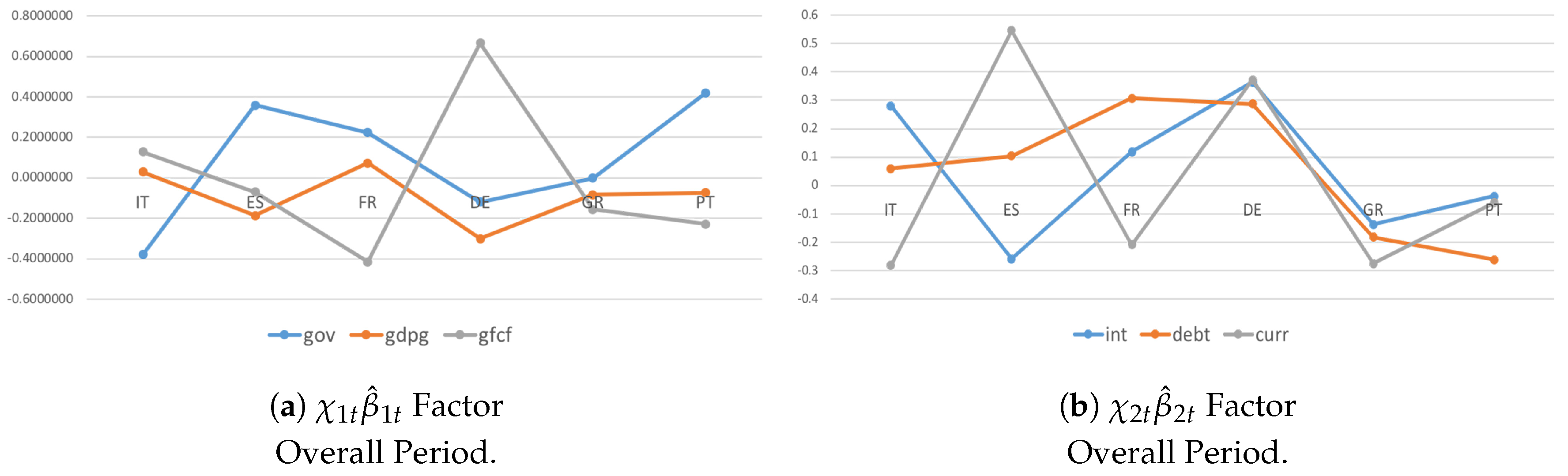
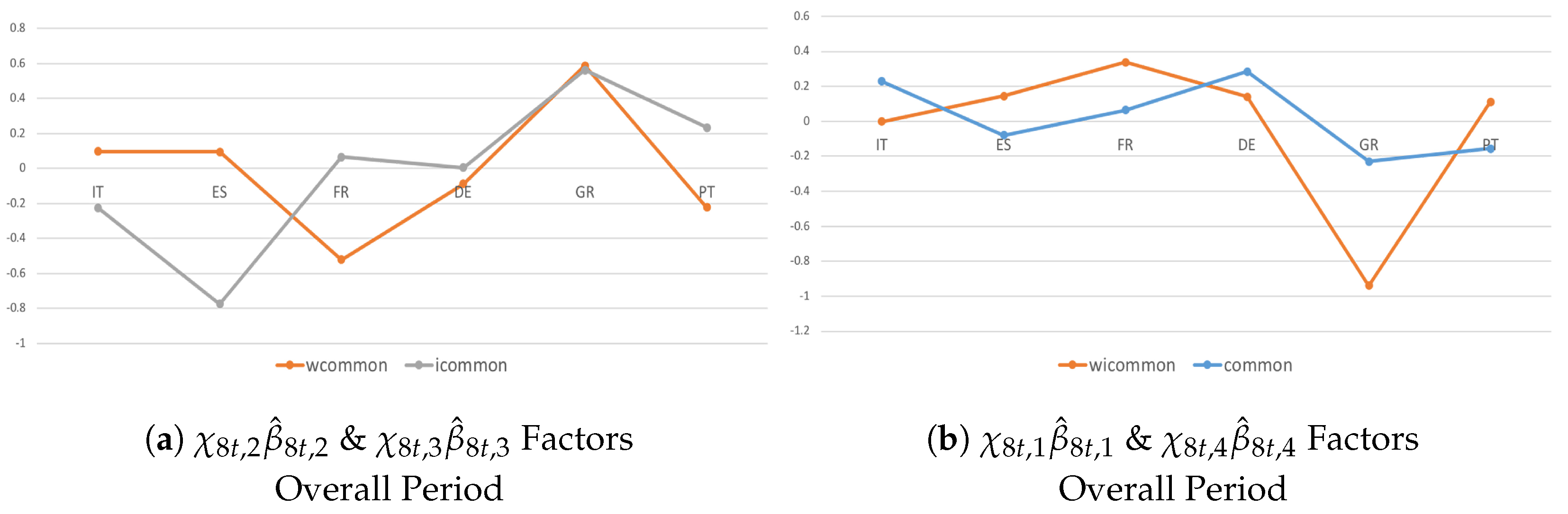
In Figure 1, where I consider the first two country-specific indicators (), there is a consistent degree of heterogeneity among countries in the financial dimension, and even more exist in the real dimension, with some common behaviors. These co-movements seem to be larger in the financial dimension (Figure 1b). In the real dimension (Figure 1a), most countries tend to be net receivers of the system; hence, unexpected country-specific shocks directly affect a country’s own output growth in the financial dimension and then in the real economy because of consistent cross-country interdependencies. It confirms the need to account for additional economic issues when dealing with multicountry data.
Accounting for the and components (Figure 2), important findings and policy perspectives are derived.
Focusing on only the component (Figure 2a,b), a consistent degree of commonality emerges in the real dimension, and even more exists in the financial dimension. Two main results follow from this. First, from a modeling perspective, the transmission tends to be more intense among countries in the financial dimension than in the real dimension. Second, from a policy perspective, the consolidations tend to occur simultaneously over time behind more coordinated fiscal actions across Euro-area countries. The spread and the intensification of spillovers increase because of the effect of additional shock transmission channels. It highlights the accuracy of the model estimated in Equation (32) when dealing with problems of unobserved heterogeneity.
The results of accounting for either the or components (Figure 2c,d) confirm the above findings. Most countries tend to be net receivers in the real economy and net senders in the financial dimension, and thus, shock transmissions are larger among capital flows than trade exposures. Cross-country homogeneity and co-movements in the financial dimension tend to be driven by stringent institutional constraints (see, e.g., Eichengreen and Wyplosz (1998) and Buti et al. (1998)), and this is proved by the intensification of the SCs. From a policy perspective, despite its large size, Germany has a limited role in generating growth spillovers. This result, in part, reflects Germany’s own dependence on growth in the rest of the Eurozone.
Different results are found for the variable-specific factors (Figure 3). To be more precise, accounting for only the component (Figure 3a), on average, countries tend to generate larger outward growth spillovers () in the financial dimension than in the real economy (). The results confirm the consistent role of capital income flows in absorbing the effects of variable-specific shocks in contrast to standard theoretical models (see, e.g., Gordon and Bovenberg (1996) and Sorensen and Yosha (1998)).
Matching both and components (Figure 3b), outward and inward growth spillovers follow a heterogeneous pattern across Euro-area countries, except Spain (possibly due to larger capital exposures). From a policy perspective, a reason could be that highly indebted countries were forced into equally taking wide-ranging austerity measures, with lost access to the financial markets. This led to a call for stronger cross-country differentiation and for temporary stimulus measures in countries not facing financial market pressure. From a modeling perspective, the analyses show the ability of the model to deal with mis-specified estimates caused by unobserved heterogeneity.
In Figure 4, I consider the last factor, . The analysis confirms the importance of accounting for economic–institutional interdependencies in real and financial dimensions. In fact, a stronger commonality is verified in Figure 4b, in which I investigate co-movements across countries and variables with and without the and components. Given an unexpected shock, the spillover effects tend to spill over in a similar manner but with greater intensification when accounting for both components. The analysis confirms that in the Euro-area countries, structural reforms without coordinated national fiscal actions negatively affect the adjustment capacity of the currency union as a whole because of a high degree of divergence.
4.3. Heterogeneity and Interactions during the Crisis Period and Post-Crisis Consolidation
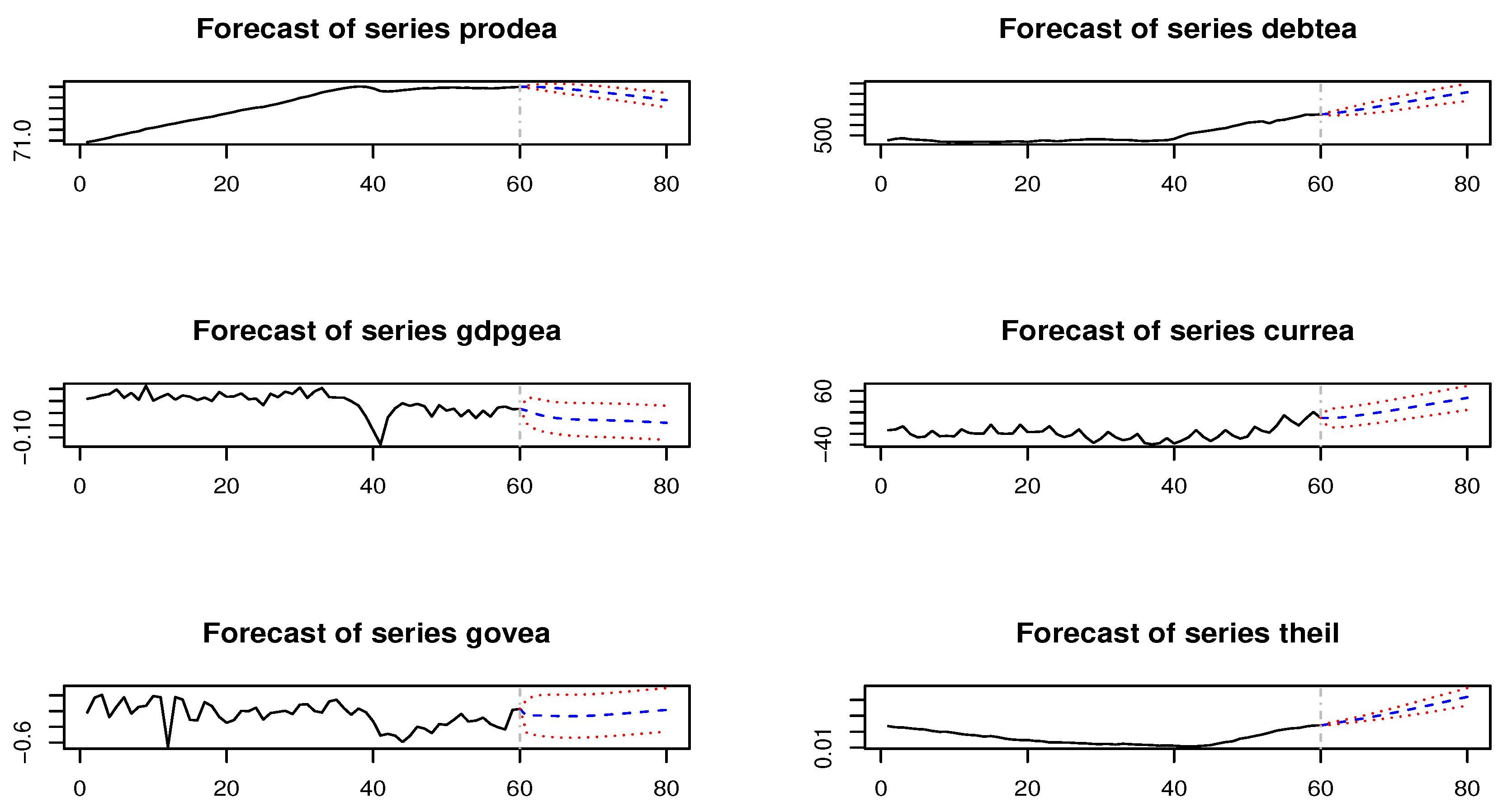
During the crisis period and post-crisis consolidation, there are deeper co-movements and a larger degree of homogeneity among countries in the real dimension and even more so in the financial dimension during the recent recession (Figure 5a,c) compared with successive post-crisis consolidations (Figure 5b,d). These results translate into three main findings. First, interdependencies due to strongly common economic–institutional linkages matter more during triggering events. Second, coordinated fiscal actions do not necessarily yield better outcomes. Third, the sign of growth spillovers is not significant in determining whether coordination should lead to a more expansionary or more restrictive fiscal stance in the member states. Thus, although recent theoretical studies suggest that the imbalances have been reduced and that macroeconomic policy mixed with a discretionary fiscal expansion and a neutral monetary policy are likely to mitigate output growth during a recession and successive consolidations, without the appropriate adjustment to the private and public sectors, Eurozone imbalances and different degrees of productivity growth will tend to persist in the future (Figure 6).
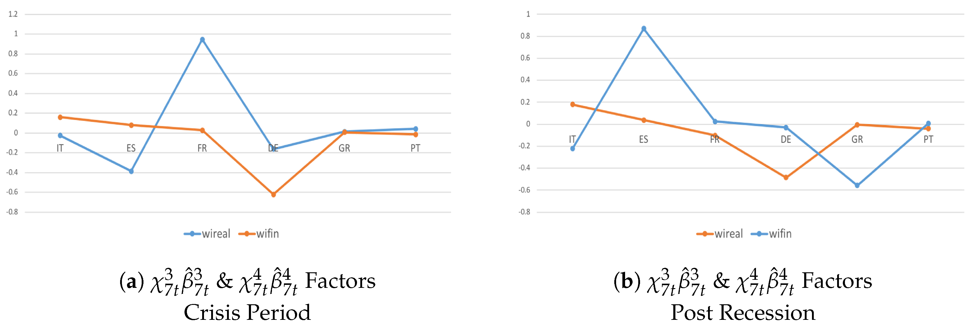
By accounting for the variable-specific indicator (Figure 7), I confirm that trade channels matter less than capital linkages. In fact, most countries tend to be net senders in the financial dimension and net receivers in the real economy. During post-crisis consolidations (Figure 7b), inward growth spillovers were more frequent and larger because of tight institutional and economic interdependencies. Thus, cross-border spillovers exacerbated the negative effects of consolidations due to (individual) domestic policies designed to counteract the events of the recession; when successive consolidations occurred, these policies proved to be ineffective and counter-productive for the domestic economy.
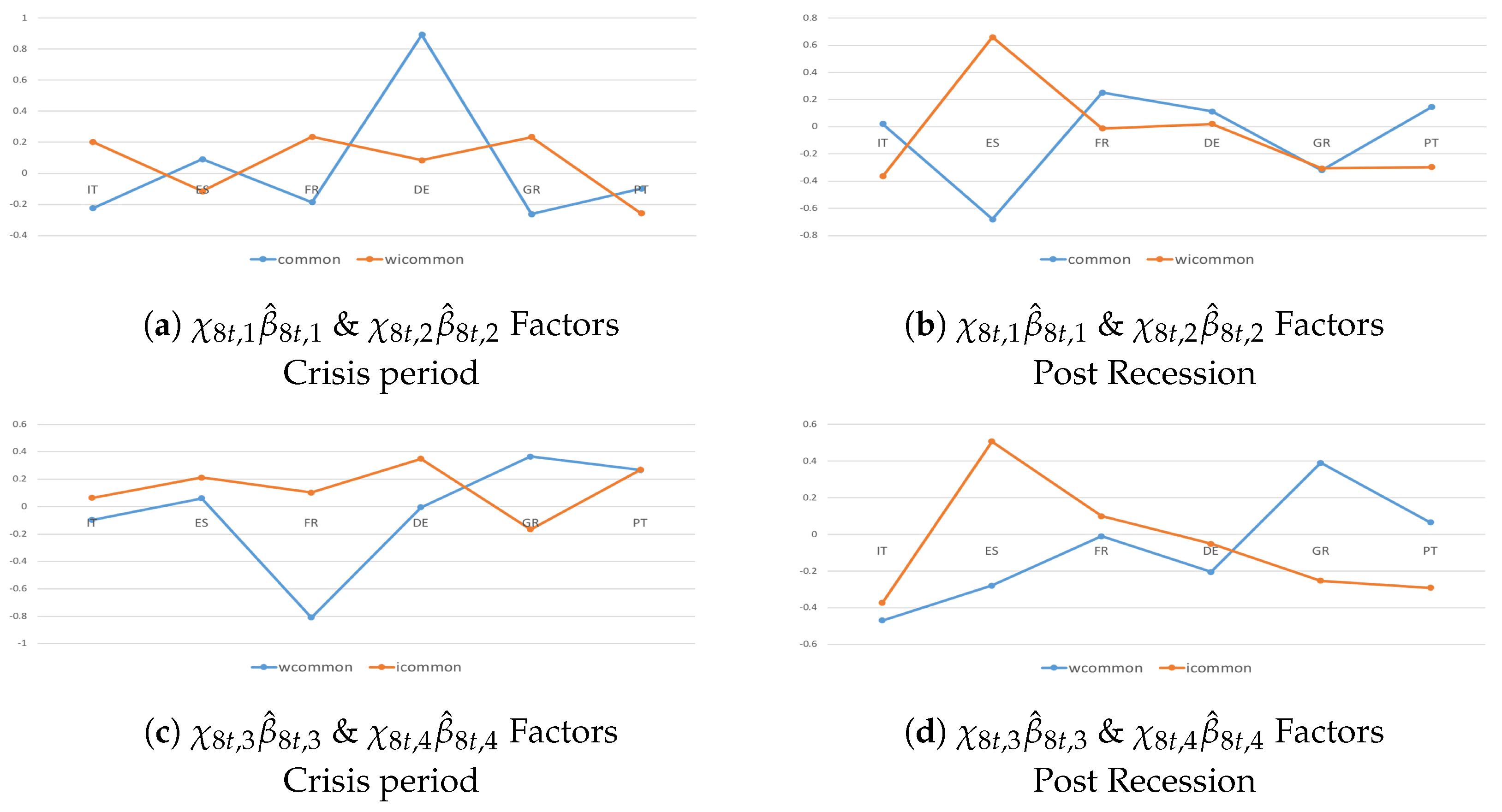
The common indicator (Figure 8) shows that economic–institutional interdependencies matter more than different transmission channels in driving the spread of common unexpected shocks. Moreover, contrary to the country- and variable-specific shocks, I observed that common shocks tended to spill over in a heterogeneous way during the recent recession (Figure 8a,b), while a larger homogeneous pattern occurred during successive consolidations, although with a different magnitude (Figure 8c,d). From a policy perspective, one reason could be that several countries actually started to put a fiscal consolidation package into practice, and national fiscal actions were adopted in a somewhat coordinated way.
5. Concluding Remarks
This paper provides an overview of a time-varying Structural Panel Bayesian VAR model to deal with model misspecification and unobserved heterogeneity problems in an applied macroeconomic analysis when studying time-varying relationships and dynamic interdependencies between different countries and sectors. I define a hierarchical prior specification strategy and describe MCMC simulations to calculate posterior distributions of CGIRFs and CF reacting to unexpected perturbations in the innovations of factors in the system. Bayesian methods are used to reduce the dimensionality of the model, structure the time variations, and evaluate issues of endogeneity. I further present a SNLR model that I built to work with smaller systems in which the regressors are observable, directly measured, and time-varying linear combinations of the right-hand variables of the time-varying SPBVAR. The advantage of this approach is that it is easier to match endogenous variables with additional time-variant factors. Here, the framework is valid if and only if prior specifications are satisfied and a fully hierarchical structure is provided. Thus, an analysis of joint and conditional densities and a sequential factorization are required.
The methodological implementation pursued in this study consists of extending the model developed in Ciccarelli et al. (2018) and thus their flexible factorization to add more time-varying endogenous factors to the system that affect the variables of interest in different time periods. The idea is that shock transmissions and economic–institutional linkages affect spillover effects among countries and variables over time and depend on a set of directly observed and hidden factors, respectively. By comparing these factors and by allowing each country to load them, model misspecification and unobserved heterogeneity problems can be investigated. For example, I can assess how the dimension and intensification of spillovers over time affect commonality, interdependence, and heterogeneity among countries and variables; interdependencies in cross-country business cycles; how different transmission channels essentially affect the spread of spillovers in macroeconomic–financial linkages given an unexpected shock; and the importance of economic and institutional implications in driving shock transmission.
An empirical application of the model to a pool of developed European economies is presented in this paper to illustrate the functioning and the ability of the model, with particular attention paid to the recent recession and post-crisis consolidation. The paper builds on three macroeconomic questions that are underdeveloped in the literature when dealing with multicountry data. First, I examine how commonality, interdependence, and heterogeneity among countries and variables change over time due to an unexpected common shock. Second, I query how additional shock transmissions affect the spread and the intensification of structural spillovers in real and financial dimensions. Third, I probe the extent to which economic–institutional linkages matter when studying co-movements and interdependencies among different countries and sectors.
The empirical analysis is robust and consistent with the more recent business cycle studies, which recognize the importance of (1) accounting for both group-specific and global factors when evaluating cross-country spillovers and (2) separating common shocks from the propagation of country- and variable-specific shocks when studying economic–financial linkages.
From a modeling perspective, I confirm that growth shocks spill over in a heterogeneous way among countries, although a significant common component holds, mainly during the crisis period and even more so during post-crisis consolidations. Over time, commonalities are stronger in the financial dimension, where shock transmission is more intense. Although recent theoretical studies suggest that the imbalances have been reduced and that macroeconomic policy mixed with a discretionary fiscal expansion and a neutral monetary policy are likely to mitigate output growth during recessions and successive consolidations, without the appropriate adjustment to the private and public sector, Eurozone imbalances and different degrees of productivity growth will tend to persist in the future.
From a policy perspective, despite a currency union, different country-specific developments of competitiveness, consumption, investment, and production that affect the national economy should be designed to shrink the divergence in growth among countries. With the advent of the financial crisis, fiscal expansion has been associated with smaller output growth loss, and national fiscal actions have been taken in a somewhat coordinated way. After gradual economic recovery began to be observed, several countries started to put a fiscal consolidation package into practice. Nevertheless, even though macroeconomic policy mixed with a discretionary fiscal expansion and a neutral monetary policy are likely to mitigate output growth during a recession and successive consolidations, without coordination efforts going beyond what already exists in the set of rules given in the Maastricht Treaty, Eurozone imbalances and different degrees of productivity growth will tend to persist in the future.
Funding
The APC was funded by the Knowledge Unlatched initiative.
Acknowledgments
I would like to express my deep and sincere gratitude to two anonymous referees for their useful and constructive suggestions.
Conflicts of Interest
The author declares no conflict of interest.
References
- Agudze, Komla Mawulom, Monica Billio, Roberto Casarin, and Francesco Ravazzolo. 2018. Markov Switching Panel with Network Interaction Effects. CAMP Working Paper Series No 1/2018. Oslo, Norway: Norwegian Business School. [Google Scholar]
- Albert, James H., and Siddhartha Chib. 1993. Bayes inference via gibbs sampling of autoregressive time series subject to markov mean and variance shifts. Journal of Business and Economic Statistics 11: 1–15. [Google Scholar]
- Beetsma, Roel, and Massimo Giuliodori. 2011. The effects of government purchase shocks: Review and estimates for the eu. Economic Journal 121: F4–F32. [Google Scholar] [CrossRef]
- Billio, Monica, Roberto Casarin, Francesco Ravazzolo, and Herman K. Van Dijk. 2016. Interconnections between eurozone and us booms and busts: A bayesian panel markov-switching var model. Journal of Applied Econometrics 31: 1352–70. [Google Scholar] [CrossRef]
- Buti, Marco, Daniele Franco, and Hedwig Ongena. 1998. Fiscal discipline and flexibility in emu: The implementation of the stability and growth pact. Oxford Review of Economic Policy 14: 81–97. [Google Scholar] [CrossRef]
- Canova, Fabio, and Matteo Ciccarelli. 2004. Forecasting and turning point predictions in a bayesian panel var model. Journal of Econometrics 120: 327–59. [Google Scholar] [CrossRef]
- Canova, Fabio, and Matteo Ciccarelli. 2009. Estimating multicountry var models. International Economic Review 50: 929–59. [Google Scholar] [CrossRef]
- Canova, Fabio, Matteo Ciccarelli, and Eva Ortega. 2007. Similarities and convergence in g7 cycles. Journal of Monetary Economics 54: 850–78. [Google Scholar] [CrossRef]
- Canova, Fabio, Matteo Ciccarelli, and Eva Ortega. 2012. Do institutional changes affect business cycles? Journal of Economic Dynamics and Control 36: 1520–33. [Google Scholar] [CrossRef]
- Canova, Fabio, and Jane Marrinan. 1997. Sources and propagation of international output cycles: Common shocks or transmission? Journal of International Economics 46: 133–66. [Google Scholar] [CrossRef]
- Carter, Chris K., and Robert Kohn. 1994. On gibbs sampling for state space models. Biometrika 81: 541–53. [Google Scholar] [CrossRef]
- Chib, Siddhartha. 1995. Marginal likelihood from the gibbs output. Journal of the American Statistical Association 90: 1313–21. [Google Scholar] [CrossRef]
- Chib, Siddhartha. 1996. Calculating posterior distributions and model estimates in markov mixture models. Journal of Econometrics 75: 79–97. [Google Scholar] [CrossRef]
- Chib, Siddhartha, and Edward Greenberg. 1995a. Hierarchical analysis of sur models with extensions to correlated serial errors and time-varying parameter models. Journal of Econometrics 68: 409–31. [Google Scholar] [CrossRef]
- Chib, Siddhartha, and Edward Greenberg. 1995b. Understanding the metropolis-hastings algorithm. The American Statistician 49: 327–35. [Google Scholar]
- Chib, Siddhartha, and Ivan Jeliazkov. 2001. Marginal likelihood from the metropolis–hastings output. Journal of the American Statistical Association 96: 270–81. [Google Scholar] [CrossRef]
- Ciccarelli, Matteo, Eva Ortega, and Maria T. Valderrama. 2018. Commonalities and cross-country spillovers in macroeconomic-financial linkages. Journal of Macroeconomics 16: 231–75. [Google Scholar] [CrossRef]
- Ciccarelli, Matteo, and Alessandro Rebucci. 2007. Measuring contagion using a bayesian time-varying coefficient model. Journal of Financial Econometrics 5: 285–320. [Google Scholar] [CrossRef]
- Cogley, Timothy, and Thomas J. Sargent. 2005. Drifts and volatilities: Monetary policy and outcomes in the post wwii u.s. Review of Economic Dynamics 8: 262–302. [Google Scholar] [CrossRef]
- Crespo-Cuaresma, Jesus, and Octavio Fernandez-Amadorb. 2013. Business cycle convergence in emu: A first look at the second moment. Journal of Macroeconomics 37: 265–84. [Google Scholar] [CrossRef]
- De Mol, Christine, Domenico Giannone, and Lucrezia Reichlin. 2008. Forecasting using a large number of predictors: Is bayesian regression a valid alternative to principal components? Journal of Econometrics 146: 318–28. [Google Scholar] [CrossRef]
- Dees, Stephane, Filippo di Mauro, M. Hashem Pesaran, and L. Vanessa Smith. 2007. Exploring the international linkages of the euro area: A global var analysis. Journal of Applied Econometrics 22: 1–38. [Google Scholar] [CrossRef]
- Degiannakis, Stavros, David Duffy, George Filis, and Alexandra Livada. 2016. Business cycle synchronisation in emu: Can fiscal policy bring member-countries closer? Economic Modelling 52: 551–63. [Google Scholar] [CrossRef]
- Doan, Thomas, Robert Litterman, and Christopher Sims. 1984. Forecasting and conditional projection using realistic prior distributions. Econometric Review 3: 1–100. [Google Scholar] [CrossRef]
- Eichengreen, Barry, and Charles Wyplosz. 1998. The stability pact: More than a minor nuisance? Economic Policy 13: 65–113. [Google Scholar] [CrossRef]
- Facchini, François, Mickael Melki, and Andrew Pickering. 2017. Labour costs and the size of government. Oxford Bulletin of Economics and Statistics 79: 251–75. [Google Scholar] [CrossRef]
- Forni, Mario, Marc Hallin, Marco Lippi, and Lucrezia Reichlin. 2000. The generalized dynami factor model: Identification and estimation. The Review of Economics and Statistics 82: 540–54. [Google Scholar] [CrossRef]
- Giannone, Domenico, Marta Banbura, and Lucrezia Reichlin. 2009. Large bayesian vector auto regressions. Journal of Applied Econometrics 25: 71–92. [Google Scholar]
- Gordon, Roger H., and A. Bovenberg. 1996. Why is capital so immobile internationally? possible explanations and implications for capital income taxation. The American Economic Review 86: 1057–75. [Google Scholar]
- Kadiyala, K. Rao, and Sune Karlsson. 1997. Numerical methods for estimation and inference in bayesian var models. Journal of Applied Econometrics 12: 99–132. [Google Scholar] [CrossRef]
- Kaufmann, Sylvia. 2010. Dating and forecasting turning points by bayesian clustering with dynamic structure: A suggestion with an application to austrian data. Journal of Applied Econometrics 25: 309–44. [Google Scholar] [CrossRef]
- Kaufmann, Sylvia. 2015. K-state switching models with time-varying transition distributions. does loan growth signal stronger effects of variables on inflation? Journal of Econometrics 187: 82–94. [Google Scholar] [CrossRef]
- Koop, Gary. 1996. Parameter uncertainty and impulse response analysis. Journal of Econometrics 72: 135–49. [Google Scholar] [CrossRef]
- Krolzig, Hans-Martin. 1997. Markov Switching Vector Autoregressions: Modelling, Statistical Inference and Application to Business Cycle Analysis. Berlin, Germany: Springer. [Google Scholar]
- Krolzig, Hans-Martin. 2000. Predicting Markov-Switching Vector Autoregressive Processes. Nuffield College Economics Working Papers 2000-WP31. Oxford, UK: Nuffield College Oxford University. [Google Scholar]
- Lane, Philip R., and Gian Maria Milesi-Ferretti. 2007. The external wealth of nations mark ii: Revised and extended estimates of foreign assets and liabilities, 1970–2004. Journal of International Economics 73: 223–50. [Google Scholar] [CrossRef]
- Litterman, Robert B. 1985. Ljung, l. and soderstrom, t. Automatica 21: 25–38. [Google Scholar]
- Litterman, Robert B. 1986. Forecasting with bayesian vector autoregressions five years of experience. Journal of Business and Economic Statistics 4: 25–38. [Google Scholar]
- Mastrogiacomo, Mauro, Nicole M. Bosch, Miriam D. Gielen, and Egbert L. Jongen. 2017. Heterogeneity in labour supply responses: Evidence from a major tax reform. Oxford Bulletin of Economics and Statistics 79: 769–96. [Google Scholar] [CrossRef]
- Pesaran, Hashem M., and Yongcheol Shinb. 1998. Generalized impulse response analysis in linear multivariate models. Economics Letters 58: 17–29. [Google Scholar] [CrossRef] [Green Version]
- Pesaran, M. Hashem, Til Schuermann, and Scott M. Weiner. 2004. Modelling regional interdependencies using a global error correcting macroeconometric model. Journal of Business and Economic Statistics 22: 129–62. [Google Scholar] [CrossRef]
- Reinhart, Carmen M., and Kenneth S. Rogoff. 2009. The aftermath of financial crises. American Economic Review 99: 466–72. [Google Scholar] [CrossRef]
- Sims, Christopher A., and Tao Zha. 1998. Bayesian methods for dynamic multivariate models. International Economic Review 39: 949–68. [Google Scholar] [CrossRef]
- Sims, Christopher A., and Tao Zha. 2006. Were there regime switches in U.S. monetary policy? American Economic Review 96: 54–81. [Google Scholar] [CrossRef]
- Sorensen, Bent E., and Oved Yosha. 1998. International risk sharing and european monetary unification. Journal of International Economics 45: 211–38. [Google Scholar] [CrossRef]
| 1 | Hidden or Latent factors are variables that are not directly observed but are rather inferred from other variables that are observed and, hence, directly measured. |
| 2 | To be more precise, if the elements of , , and are stacked over i, it is possible to obtain matrices that are not block-diagonal for at least some l. |
| 3 | The vec operator transforms a matrix into a vector by stacking the columns of the matrix, one underneath the other. |
| 4 | A proxy variable is an easily measurable variable that is used in place of a variable that cannot be (directly) measured or is difficult to measure. |
| 5 | The Wishart distribution is a multivariate extension of distribution and, in Bayesian statistics, corresponds to the conjugate prior of the inverse-covariance matrix of a multivariate normal random vector. |
| 6 | The Gamma Distribution is a two-parameter family of continuous probability distributions that provides the probabilities of occurrence of different possible outcomes in an experiment. |
| 7 | For instance, the Minnesota priors are based on an approximation that involves replacing with an estimate, . See, e.g., Doan et al. (1984) and Litterman (1986). |
| 8 | These implementations do not allow for the use of the Minnesota prior since its covariance matrix is written in terms of blocks that vary across equations. |
| 9 | See, e.g., Chib and Greenberg (1995b). |
| 10 | The component corresponds to the sum of and . |
| 11 | Own computations. |
| 12 | The conditional projection for output growth is the one that the model would have obtained over the same period conditionally on the actual path of unexpected shock for that period. |
| 13 | The unconditional projection is the one that the model would obtain for output growth for that period only on the basis of historical information, and it is consistent with a model-based forecast path for the other variables. |
Figure 1.
Systemic Contributions of the given a shock to real and financial dimensions are drawn as standard deviations of the variables in the system and in year-on-year growth rates. They account for (plot a) and (plot b) cross-country indicators, where and are posterior means.
Figure 1.
Systemic Contributions of the given a shock to real and financial dimensions are drawn as standard deviations of the variables in the system and in year-on-year growth rates. They account for (plot a) and (plot b) cross-country indicators, where and are posterior means.

Figure 2.
Systemic Contributions of the given a shock to real and financial dimensions are drawn as standard deviations of the variables in the system and in year-on-year growth rates. They account for (plot a), (plot b), (plot c), and (plot d) cross-country indicators, where , , , and are posterior means.
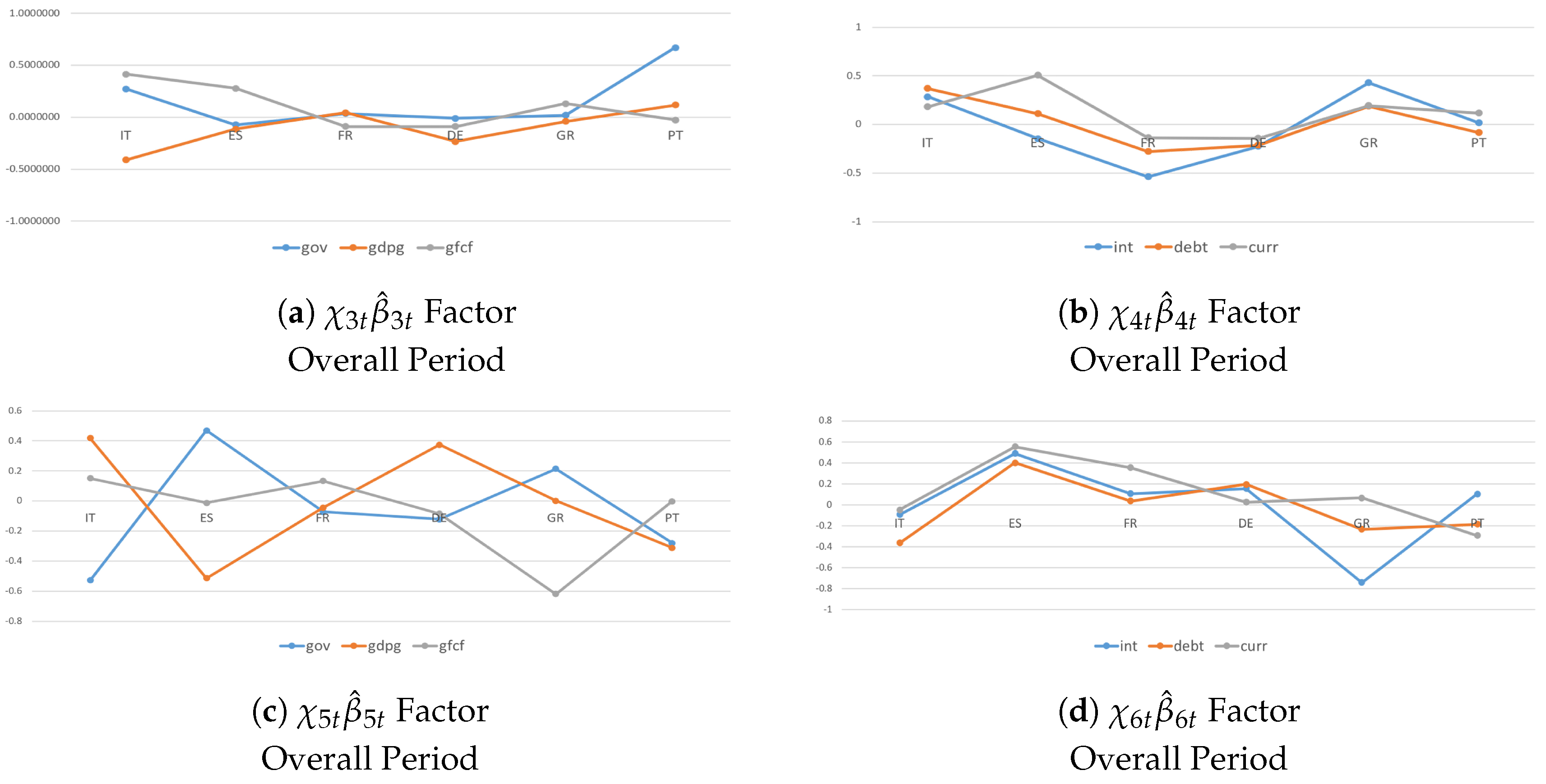
Figure 3.
Systemic Contributions of the given a shock to real and financial dimensions are drawn as standard deviations of the variables in the system and in year-on-year growth rates. They account for (plot a), (plot a), (plot b), and (plot b) variable-specific indicators, where ’s are posterior means.
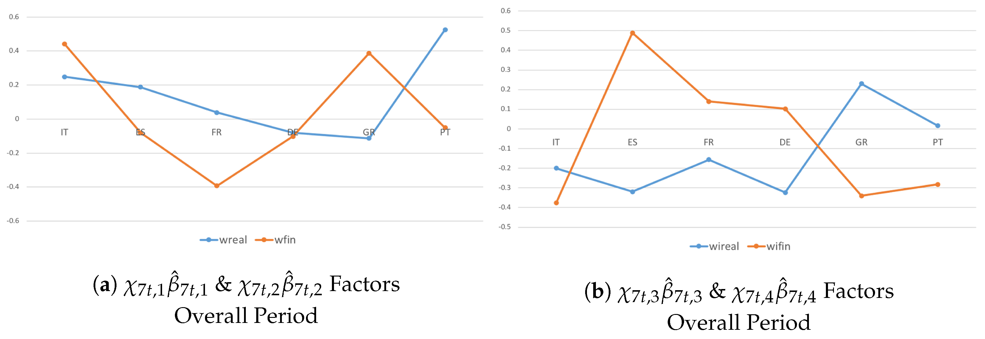
Figure 4.
Systemic Contributions of the given a shock to real and financial dimensions are drawn as standard deviations of the variables in the system and in year-on-year growth rates. They account for (plot b), (plot a), (plot a), and (plot b) common indicators, where ’s are posterior means.
Figure 4.
Systemic Contributions of the given a shock to real and financial dimensions are drawn as standard deviations of the variables in the system and in year-on-year growth rates. They account for (plot b), (plot a), (plot a), and (plot b) common indicators, where ’s are posterior means.

Figure 5.
Systemic Contributions of the given a shock to real and financial dimensions are drawn as standard deviations of the variables in the system and in year-on-year growth rates, focusing on the recent financial crisis (plots a,c) and post-crisis consolidation (plots b,d) periods. They account for and cross-country indicators, where and are posterior means.
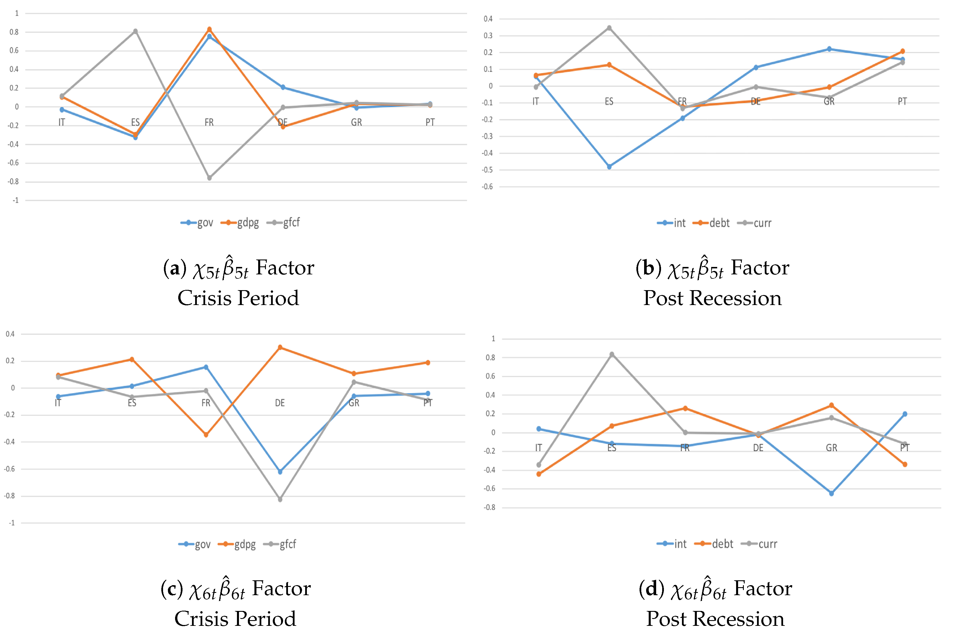
Figure 6.
The figure draws CF of the productivity, general government debt, real GDP growth rate, current account balance, general government spending, and the generalized entropy index from to . The latter corresponds to Theil’s Entropy and is computed by weighing the GDP with the population in terms of proportions with respect to the total. It can be viewed as a measure of divergence and economic inequality. Here, forecasts from to correspond to conditional projections of each variable drawn in the .

Figure 7.
Systemic Contributions of the given a shock to real and financial dimensions are drawn as standard deviations of the variables in the system and in year-on-year growth rates, focusing on the recent financial crisis (plot a) and post-crisis consolidation period (plot b). They account for and variable-specific indicators, where and are posterior means.

Figure 8.
Systemic Contributions of the productivity given a shock to real and financial dimensions are drawn as standard deviations of the variables in the system and in year-on-year growth rates, focusing on the recent financial crisis (plots a,c) and post-crisis consolidation (plots b,d) periods. They account for , , , and common indicators, where ’s are posterior means.


Table 1.
Diagnostic Tests.
| Test | Test Statistics | Degrees of Freedom | p-Value |
|---|---|---|---|
| 5665 | 2430 | 0.00 | |
| 526.51 | 540 | 0.6531 | |
| 29.41 | 12 | 0.00342 |
Here, stands for a Multivariate Ljung-Box Test of the series, with lags ; refers to the Portmanteau (Asymptotic) Test on the residuals, with lags ; is the Marginal (Conditional) Likelihood Estimation Test obtained through the Schwartz approximation, with .
Table 2.
Structural Spillover Matrix.
| Shock/Response | … | To Others | |||
|---|---|---|---|---|---|
| … | |||||
| … | |||||
| ⋮ | ⋮ | ⋮ | ⋱ | ⋮ | ⋮ |
| … | |||||
| From Others | … |
Note: Row variables are the origin of the unexpected shock. Column variables are the respondents or spillover receivers.
© 2019 by the author. Licensee MDPI, Basel, Switzerland. This article is an open access article distributed under the terms and conditions of the Creative Commons Attribution (CC BY) license (http://creativecommons.org/licenses/by/4.0/).
Share and Cite
MDPI and ACS Style
Pacifico, A. Structural Panel Bayesian VAR Model to Deal with Model Misspecification and Unobserved Heterogeneity Problems. Econometrics 2019, 7, 8. https://0-doi-org.brum.beds.ac.uk/10.3390/econometrics7010008
AMA Style
Pacifico A. Structural Panel Bayesian VAR Model to Deal with Model Misspecification and Unobserved Heterogeneity Problems. Econometrics. 2019; 7(1):8. https://0-doi-org.brum.beds.ac.uk/10.3390/econometrics7010008
Chicago/Turabian StylePacifico, Antonio. 2019. "Structural Panel Bayesian VAR Model to Deal with Model Misspecification and Unobserved Heterogeneity Problems" Econometrics 7, no. 1: 8. https://0-doi-org.brum.beds.ac.uk/10.3390/econometrics7010008
Note that from the first issue of 2016, this journal uses article numbers instead of page numbers. See further details here.