A Semi-Parametric Approach to the Oaxaca–Blinder Decomposition with Continuous Group Variable and Self-Selection

Levy Economics Institute, Bard College, Annandale-on-Hudson, NY 12504, USA
Econometrics 2019, 7(2), 28; https://0-doi-org.brum.beds.ac.uk/10.3390/econometrics7020028
Submission received: 22 February 2019
/
Revised: 19 May 2019
/
Accepted: 18 June 2019
/
Published: 21 June 2019
Abstract
:This paper presents an extension to the Oaxaca–Blinder decomposition with continuous groups using a semiparametric approach known as varying coefficients model. To account for potential self-selection into the continuum of groups, the use of inverse mills ratios is expanded upon following the literature on endogenous selection. The flexibility of this methodology may allow detecting heterogeneity when analyzing endogenous dose treatments effects, as well as correcting for endogeneity when analyzing the heterogeneous partial effects across the continuous group variable. For illustration, the methodology is used to revisit the impact of body weight on wages, using body mass index (BMI) as the continuum of groups, finding evidence that body weight has a negative, but decreasing impact on wages for both white men and women.
Keywords:
Oaxaca–Blinder Decomposition; heckman selection; semi-parametric; endogeneity; kernel; non-linear; BMI; Body weight; wages differentialsJEL:
C14; I19; J31; J71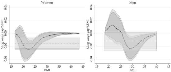
1. Introduction
Since the seminal papers from Blinder (1973) and Oaxaca (1973), many studies have used what is known as the Oaxaca–Blinder (OB) decomposition for analyzing outcomes differences between two well defined groups. Such differences are characterized as functions of differences in characteristics (composition effect) and differences in coefficients associated with those characteristics (wage structure effect). Subsequent research provided refinements that extended the OB decomposition analysis to non-linear functions, distributional statistics other than the mean, as well as strategies to identify the model when some of the underlying assumptions do not hold (see Fortin et al. (2011) for a review of other methodological extensions).
While the OB decomposition can be directly applied to scenarios with naturally discrete groups (i.e., union and non-union workers, men and women, whites and nonwhites), the application of OB type decompositions on cases with continuous or quasi-continuous groups is not standard. Ñopo (2008) and Ulrick (2012) have proposed extensions to the standard OB decomposition allowing for a continuous group variable, using ad hoc parametric approximations.1 These strategies can be biased if the selected functional form is incorrect, and neither strategy deals with a scenario where there is self-selection of individuals into groups based on unobservables (endogenous membership).
The purpose of this paper is to extend the OB decomposition allowing for a continuous group variable using a semiparametric approach known as varying coefficient models (Hastie and Tibshirani 1993).2 The strategy accounts for endogenous self-selection into groups abstracting from a generalization of the Heckman selection model that uses generalized inverse mills ratios (GIMR) or generalized residuals (Heckman 1979; Lee 1978; Li and Racine 2007; Vella 1998) to address the problem. As discussed in Wooldridge (2015), the use of GIMR is equivalent to using a control function approach when addressing endogeneity.
A thorough search of the relevant literature yielded only two other papers that discuss the estimation of varying coefficient models with this type of endogeneity. Centorrino and Racine (2017) propose a strategy that uses instrumental variables and method of moments to address endogeneity and estimate the varying coefficient models using sieve estimators. More recently, Delgado et al. (2019) developed an estimator based on a control function approach, using a combination of spline regressions for the estimation of the first stage residuals, and kernel regressions for the identification of the coefficients in the model. The strategy proposed here is closer to Delgado et al. (2019) which generalized residuals from a first stage auxiliary regression, the generalized inverse mills ratios, are included in the main model before it is estimated using local linear kernel regression methods.
The strategy presented could be used for analyzing heterogeneous dose-treatment effects under endogeneity, using an OB decomposition framework. In addition, under the assumption that all other control variables are exogenous, the proposed strategy can also be used to identify the parameters of the model of interest and analyze the heterogeneity of the impact of characteristics across the continuous group variable. For example, Centorrino and Racine (2017) re-explore the impact of race, experience and place of residence on wages when looking at individuals with different levels of education (equivalent the continuous grouping variable). Delgado et al. (2019) illustrate their methodology analyzing the demand for gasoline in the US using household income as the grouping variable. Other applications may include the analysis of smoking and smoking intensity on wages (Hotchkiss and Pitts 2013), training duration on employment probabilities (Kluve et al. 2012), or as will be shown in the illustration section, the impact of Body Mass Index (BMI) on wages (Cawley 2004).
The subsequent sections of the paper are structured as follows. Section 2 describes the basic Oaxaca–Blinder decomposition analysis in the presence of self-selection/endogenous membership. Section 3 introduces the use of the Generalized Inverse Mills Ratio (GIMR), when individuals self-select into continuous group. Section 4 describes the estimation of varying coefficient models, selection of bandwidths and the estimation of standard errors. Section 5 provides Monte-Carlo Simulations showing the performance of the proposed strategy. Section 6 provides an example of the implementation of the methodology revisiting the wage penalty of obesity based on the research of Cawley (2004). Section 7 concludes the paper.
2. The OB Decomposition with Selection: Basics
In the standard OB approach, the goal is to analyze how differences in observed characteristics, and returns to these characteristics, explain average differences on outcomes between two groups. For the appropriate identification of the OB decomposition, the strategy requires that potential outcomes can be estimated using two well-specified linear models with exogenous membership into each group. This ensures that the distribution of the errors is orthogonal to the group membership.
In many instances, however, the assumption of membership exogeneity is likely to be violated if individuals self-select to be part of a specific group (i.e., part of the treatment group).3 When this happens the conditional distribution of the errors is no longer independent of the group membership, ruling out the identification strategy of the standard decomposition approach. A strategy commonly used to address this problem is the implementation of a Heckman Selection model.
As described in Heckman (1979), endogenous selection can be considered as an omitted variable problem that can be corrected by modeling the selection process and using this information to identify the parameters of the model of interest.4 This strategy requires the estimation of a three-equation model that is described as follows:
where is the latent propensity of an individual i to be part of group B, is a set of exogenous variables uncorrelated with and , and is a vector of variables related to individuals membership that may include variables not included in X.5 If we assume that () are jointly distributed as multivariate normal:
the model can be estimated using a full information maximum likelihood (FIML) or a two-step procedure (heckit). The latter involves including estimates for the selection correction terms, the inverse mills ratio (IMR), in the main outcome model based on the information from the selection equation. For this setup, the IMR ( is defined as follows:
where stands for the normal density function, and for the normal cumulative density function.
The parameters can be obtained by estimating the selection equation in (1) using a probit model, while unbiased estimations for outcome equations can be obtained using ordinary least squares (OLS) by including the corresponding IMR as explanatory variables:
In this setting, an estimation of the outcome gap after adjusting for selection can be written as follows:
which can be used to implement any variation of the standard OB decomposition based on assumptions of the counterfactual wage structure.6 As described in Fortin et al. (2011), outcome differences accounted for by differences in the coefficients (structure effect) can be interpreted as the treatment effect of membership, after adjusting for differences in observed characteristics and endogenous selection. In addition, under the exogeneity assumption of the explanatory variables , the detailed decomposition can be used to analyze the heterogeneity of the contribution individual characteristics on the outcome gap.
3. Generalized Sample Selection
The model described above assumes that the only information known about the selection process is that individuals are members of one of two groups (A or B). As discussed in Vella (1998), may contain additional information that can be used to obtain a better approximation of the selection correction term, even if the interest remains in analyzing differences between two groups.
As before, consider a model where the continuous characteristic is observed for each individual, which can reference their membership status to a continuum of groups. This information can be used to broadly classify individuals into Groups A and B (dichotomization of the groups). The selection process and outcome equations can be described as follows:
with following a joint normal distribution as defined previously, with some arbitrary threshold to define membership, and with the third Equation in (7) representing the equation, or equations, that describe the endogenous selection process. This model reverts to the standard switching regression model if a dichotomous transformation is used as described in the previous section. However, if further variation in is observed, other methods can be used to exploit this information.
Many authors have proposed alternatives for the estimation of these types of selection models where more information about the endogenous membership is available, using both parametric and semiparametric strategies (see Li and Racine (2007, sct. 10.3), and Vella (1998)). In general, following the approach proposed by Heckman (1979), these methodologies suggest that to obtain consistent estimators for the parameters , one should include an approximation of the selection bias term as a control in the main regression model. This paper concentrates on three methodologies that assume the overall distribution of is observed, but can be easily adapted to scenarios where is partially observed.
Vella (1998) discusses the estimation of models such as the one described above and suggests that a feasible strategy is to estimate the selection process as a tobit model if has a censored distribution.7 In this case, assuming is censored at zero, the corresponding IMR (selection correction term) is defined as:
These are often called generalized residuals, and are referred here as generalized inverse mills ratios (GIMR). It should be noted when is not censored, the selection equation can be estimated using standard OLS and the IMR are simply the OLS residuals. Alternatively, this equation can be modified if is censored at different points of its distribution. Including these residuals in the main model is equivalent to the control function described in Wooldridge (2015). Control function approach is also a common strategy for dealing with endogeneity in linear and nonlinear parametric frameworks, and in nonparametric frameworks (see Li and Racine (2007, chp. 17), Henderson and Parmeter (2015, chp. 10), and Wooldridge (2015)).
As Vella (1998) and Li and Racine (2007) describe, using the correction term in Equation (8) provides estimations that are more stable and efficient than using the standard IMR (which assumes dichotomous grouping). However, an instrumental variable is required to identify the coefficients of the selection correction term and the grouping variable (intensity), if it were to be included in the model specification.
An alternative method described in Vella (1998) is one where the selection process corresponds to a setting with discrete but ordered selection rules. If we assume that is a discretized transformation of (i.e., ), and that is the latent propensity of an individual i to be part of group , then the selection equation process can be written as:
Note that Equation (9) is a different way of writing the selection model described in Vella (1998), where all coefficients in are permitted to vary. Additionally, note that all latent coefficients are affected by the same shock (). Under the parallel lines assumption (Williams 2016), an ordered probit (O-probit) can be used to estimate this model, where only the constant is allowed to vary across models.
As described in Chernozhukov et al. (2013), a more flexible alternatives for the estimation of the selection model is allowing all parameters in to vary across all points of the distribution of . This can be done using independent models (Foresi and Peracchi 1995), or using simultaneous models such as the generalized ordered probit model (Terza 1985). Both alternatives impose greater computational burden and may produce unrealistic predicted probabilities in the model, as the number of groups (J) increase.8
As described in Vella (1998), similar to the binary group case, the outcome equations can be consistently estimated using OLS by simply including a selection correction term, which for the selection rule described by Equations (9) takes the following form:
where is the GIMR. Here, the term is only an approximation of the correction term , as it can be considered as the expected value of the correction term for all values of within the group . Any approximation bias would disappear as the sample size increases to infinity () and the bandwidth within each category tends to zero . If no instrumental variables are used in the selection equation model, the GIMR will be strongly linear with the estimated latent index, and the estimator will be poorly identified (Chiburis and Lokshin 2007). This strategy can be easily adapted to scenarios where is partially observed due to censorship, however, a drawback is that it requires choosing the number of groups to reclassify the original data.
Taking from the literature on distributional regressions (Chernozhukov et al. 2013), the last alternative suggested here is to use global distributional regressions to characterize the cumulative distribution of the outcome . This can be done using a fractional probit model that takes the form:
Empirically, this model can be estimated by substituting with the sample unconditional cumulative distribution , or some other approximation.9 In this case, the corresponding GIMR takes the form:
Once the corresponding selection correction terms have been estimated, they can be used to estimate the parameters for the models of interest (Equation (7)) and the selectivity corrected average wage gaps. These elements can then be used to implement an OB decomposition in the standard way using Equation (6). In this framework, the structure effect can be interpreted as the average treatment effect.
As it will be shown through Monte-Carlo Simulations, all these methodologies can be used for identification of the main parameters of the model, but the correct identification of the constant in the original model will depend on the shape of the distribution of membership variable and the method of estimation of the generalized inverse mills ratios.
4. Varying Coefficient Models with Endogenous Membership
4.1. Local Kernel Estimators
The previous section described the construction of sample selection correction terms that uses the information on the intensity of the treatment/selection variable to obtain the GIMR, which can be used to correctly identify the parameters of the outcome models and implement an OB decomposition comparing two groups. In this section, we discuss the strategy that would allow us to estimate parameters corresponding to any number of groups, depending on the grouping variable .
A generalization of the selection process and outcome equations that accounts for a continuum of groups can be written as:
where is assumed to be a vector of parameters that vary with the continuous variable . Similar to the previous setup, we assume that the errors and are correlated, which implies that is endogenous, and Equation (13) cannot be directly estimated. This problem has also been discussed in Centorrino and Racine (2017) and Delgado et al. (2019), with the latter suggesting a three-step control function approach, similar to the one suggested here, to correct for this source of endogeneity.
Under the assumption that is a discreet and ordered variable, Chiburis and Lokshin (2007) implement an estimator for Equations (13) using an ordered probit to model the selection process, and OLS regressions for the outcome models for each identified group. They implement the estimators for this model for both FIML and a two-step heckit procedure.
Abstracting from Chiburis and Lokshin (2007) estimator, and based on the discussion provided in Section 2, including the GIMR term into the outcome model would allow us to obtain consistent estimates of the parameters by estimating the following equation:
where is a vector that includes the constant and explanatory variables, and is the estimate of the GIMR for person .10
In contrast with Chiburis and Lokshin (2007), if we assume that is continuous, it would be impossible to estimate the parameters in Equation (14) by running separate regressions with constraint samples.11 Borrowing from the non-parametric econometrics’ literature, feasible estimations can be obtained for the parameters using a semiparametric model known as varying coefficient models (Hastie and Tibshirani 1993; Li and Racine 2007).12 Using this strategy, one imposes no restrictions on the coefficients other than them being smooth and differentiable at .
One of the estimators for varying coefficient models expand on the use of kernel local smoothing regressions, allowing for a flexible parameterization of the outcome model in Equation (14), modeling the conditional mean as a linear function of explanatory variables and selection term conditional on . This would in principle allow us to obtain estimates of the coefficients for every point of interest:
with , and the function representing the conditional mean of any variable z in the neighborhood of d. This model can be estimated by minimizing the following objective function:
which is equivalent to minimizing the weighted squares errors of the model, with weights given by the kernel function and the bandwidth . As discussed in Hastie and Tibshirani (1993), to reduce problems with boundary bias, the recommendation is to use a local linear approximation for . The constant component of these coefficients, , represent the local effect that any variable has on the outcome in the neighborhood of . Once all the parameters in Equation (14) are identified, they can be used to implement the OB decomposition for the selectivity corrected outcome between any two particular groups, depending on assumptions regarding the reference group (Fortin et al. 2011).
4.2. Bandwidth and Standard Errors
An important aspect of the estimation of varying coefficient is the choice of bandwidth . Larger bandwidths help reduce the variance of the estimated parameters, but increase the bias. In contrast, smaller bandwidths can reduce the bias, at a cost of higher variance.13 While there are a few suggestions in the literature regarding to the choice of bandwidths (see for example Zhang and Lee (2000)), a leave-one-out Cross-validation procedure, using a single smoothing parameter for smoothing all explanatory variables, is used here. This implies choosing so that it minimizes the following expression:
where and are the leave-one-out estimators for and , for a given bandwidth h and at a point . is a weight function that is used to avoid difficulties of slow converge cause by the sparse distribution of . Because the bandwidth does not affect the calculation of the GIMR, the parameter is considered exogenous for the estimation of the Cross-validation criteria.
In the present context, the analytical estimation of the standard error of varying coefficient models with selection can be considerably cumbersome to implement. Under the assumption that the selection term is fixed and exogenous, Li and Racine (2007) provide expressions for the asymptotic distribution of the standard errors for the kernel local linear estimator of varying coefficient models.14 However, because the model described above is based on a two-step estimation process, the estimation of the standard errors needs additional adjustments (Heckman 1979).
Because of the added complexity, a more feasible method, albeit computationally intensive, is using bootstrapped standard errors with pairwise resampling (Horowitz and Lee 2012).15 The benefits of this strategy have been discussed in Yatchew (2003) and Keele (2008), and more recently, its application has been formally discussed in Cattaneo and Jansson (2018) in the framework of kernel-based semiparametric estimations. For the procedure that follows, we use the cross-validation optimal bandwidth of the original sample as fixed for each bootstrap iteration.16 The procedure can be described as follows:
- Step 1. Obtain a random paired bootstrap sample from the original sample.
- Step 2. Estimate the selection correction term using any of the methods presented in Section 2.
- Step 3. Estimate the coefficient for the outcome models for all points of interest , based on the bootstrap sample , using local kernel regressions, and the global optimal bandwidth.
- Step 4. Estimate the decomposition components for the group(s) of interest.
- Step 5. Repeat Steps 1 to 4, B times to obtain the empirical distributions of the aggregated and detailed decomposition components.
In the next section I present a Monte-Carlo Simulation to assess the performance of the proposed strategy to identify parameters of the outcome models, as well as to analyze the estimation of the confidence intervals and standard errors. After that, I provide an illustration of the methodology revising the main results from Cawley (2004), where BMI will be used as the continuum group variable.
5. Monte-Carlo Simulations
To assess the performance of the proposed methodology, and their finite sample properties, I draw simulate 1000 samples of size n = 500, 1000, 2500 and 5000, from the following scheme:
where represents a joint normal distribution. The endogenous membership is defined by:
with three separate specifications used for the varying coefficient:
where and are the standard normal probability and cumulative density functions, respectively. These functional forms were chosen to generate nonlinearities that could not be captured using polynomial approximations. Finally, to add heterogeneity on the degree of endogeneity across d, the outcome of interest is defined as:
After each sample is simulated, the model is estimated with the procedure described in Section 3, estimating the cross-validated bandwidths for each simulated sample, and estimating bootstrapped standard errors using 199 repetitions. Table 1 provides a summary of the results, showing the bias, standard errors from the simulations, average bootstrapped standard errors, and the 95% coverage and bias corrected coverage using normal based confidence intervals.
For the results in Table 1, OLS-GIMR is used to correct for endogenous selection. Table 2 provides a similar exercise, using simulations with samples of size n = 5000, but applying the GIMR from the ordered probit and fractional probit regression models. In all cases, Table 1 and Table 2 reports the average estimates for the coefficients at selected points in the distribution of , with the top and bottom values (−3 and 5) representing the 2.5th and 97.5th percentiles of the distribution of .
The simulations suggest that the proposed estimator performs reasonably well in finite samples. Akin to other applications of semiparametric analysis, the estimator presents the largest bias at the boundaries of the distribution, but also around points where the second derivative of the coefficient with respect to ( is large. This bias disappears when larger samples and smaller bandwidths are used.
The bootstrap procedure used to correct the standard errors produces estimates that slightly understates the simulated standard errors. For the simulations with samples sizes n = 500, the average bootstrapped standard errors understate the simulated standard errors by 5% in average. For the simulations with sample size of 5000, bootstrapped standard errors understate the simulated standard error in 2.5% in average. Looking at the raw coverage, except for areas with large bias, the estimator obtains coverages between 90% to 95%, even for the simulations with the smallest sample size.17 After correcting for the average bias, the coverage is above 94% for the majority of the cases. Finally, comparing the performance of the different estimators of the GIMR (Table 2), all strategies perform similarly well, with only minor differences in coverage. Additional simulations presented in the appendix show that the choice of the GIMR estimations matters if has a bounded distribution.18
6. Application: Revising the Impact of Obesity on Wages
Several studies have found that that body weight is negatively correlated with wages, in particular for white women (Cawley 2004; Sabia and Rees 2012; Averett 2011; Fikkan and Rothblum 2012). The most common explanations for the negative correlation are: obesity lowers wages by reducing productivity and increasing discrimination; low wages may cause obesity due to unhealthy eating habits caused by lower income; or that unobserved factors simultaneously cause higher body weights and lower wages. On his review of the literature, Cawley (2004) criticizes the robustness of various strategies that have been followed in the literature to analyze the relationship between body weight and wages, and suggests the application of an instrumental variable approach to better capture the causal relationship between Body Mass Index (BMI) and wages.
Using data from the National Longitudinal Survey of the Youth (NLSY) for the years 1981 to 2000, Cawley (2004) provides estimations for the impact of BMI and weight on wages, using sibling’s BMI, sex and age as instruments for own BMI.19 Correcting for reporting errors on weight and height, the evidence of his preferred model suggests that the negative effect of higher BMI on wages is only statistically significant for white women, with no statistically significant effect for other groups.
For the illustration of the proposed methodology, BMI will be considered the continuous group variable that is used to analyze the wage gaps in relation to body weight, using the same instrumental variables as Cawley (2004). Due to the higher demands that the methodology imposes on the data, some changes on the data definitions and model specifications are introduced. These changes are described next.
6.1. Replication and Variable Definition Changes
Cawley (2004) estimates instrumental variable models for six demographic groups based on gender and race, using measures for BMI that are corrected for self-reporting error20 as the main explanatory variable, and using siblings’ BMI, age and sex as instrumental variables. In his preferred model, Cawley (2004) reports that BMI has a negative impact on wages for all groups and races, but is only statistically significant for white woman. For this group, a one-point increase in BMI translates in 1.7% lower of wages.
Due to the higher demands that the semiparametric methodology imposes on the data, the original model specification required some adjustments.21 First, sampling weights are excluded from the analysis, so that clustered bootstrapped standard errors can be applied directly. Second, data with missing information in the general intelligence score, highest grade attained, job tenure and county employment rate are excluded from the sample. Father’s and mother’s highest degree of education are combined into a single variable (parent highest degree of education), and observations with missing data on both parents are also excluded from the sample. Finally, observations with a BMI below 14 and above 60 are also excluded from the sample. This reduces the total sample from 44,026 observations to 40,087 observations.
Re-estimating the results using the same specifications used in Cawley (2004), incorporating the changes described above, show that the conclusions are robust to the model and sample specification changes, with small changes in the point estimates (see Table 1). On the bottom two panels of Table 3, the main model is re-estimated including the OLS-GIMR to account for endogeneity (Wooldridge 2015). OLS-GIMR is chosen because the full distribution of BMI is observed in the data. In addition to using the Siblings data as instruments, second order interactions are also included as instruments to account for further nonlinear effects. The results using the OLS-GIMR are identical to the standard instrumental variable approach, showing only small changes when interactions are added as instruments. For the rest of the paper, linear and quadratic terms of the instrumental variables will be used to account for nonlinear effects for identification of the selection process.22
6.2. Semiparametric Oaxaca Decomposition
6.2.1. Oaxaca Decomposition Approach and Implementation
To implement an OB decomposition in the present framework, it is necessary to define an appropriate reference group to analyze wage gaps across BMI, and the appropriate way to estimate the parameters for the reference group.23 For the analysis of BMI and wages, a common approach is to use individuals with a “healthy” BMI level as the baseline group, and compare the results against other groups (over and underweight). Following this premise, people with a BMI between 18.5 and 25 are used as the reference group, and the coefficients estimated with this sample will be considered as the average coefficients for people with healthy BMI. This group represents approximately 48% of white men and 62% of white women. Using this reference group, the OB decomposition is obtained by estimating the following equations:
The first equation is estimated using the sample of the reference group only (healthy BMI), whereas the second is estimated using kernel local linear regressions as described in Section 4.1, over the whole distribution of BMI. Notice that both equations include the GIMR variable to adjust for sample selection, and that Equation (18) considers everyone, including those in the reference group.24
For the implementation of the OB decomposition, I use a threefold decomposition on the selectivity corrected wage gap, using the following formulas:
where is the local linear predicted mean of with BMI at , and is the mean of X for people with healthy BMI, and and are the estimated coefficients corresponding to the reference group and for people with BMI around .
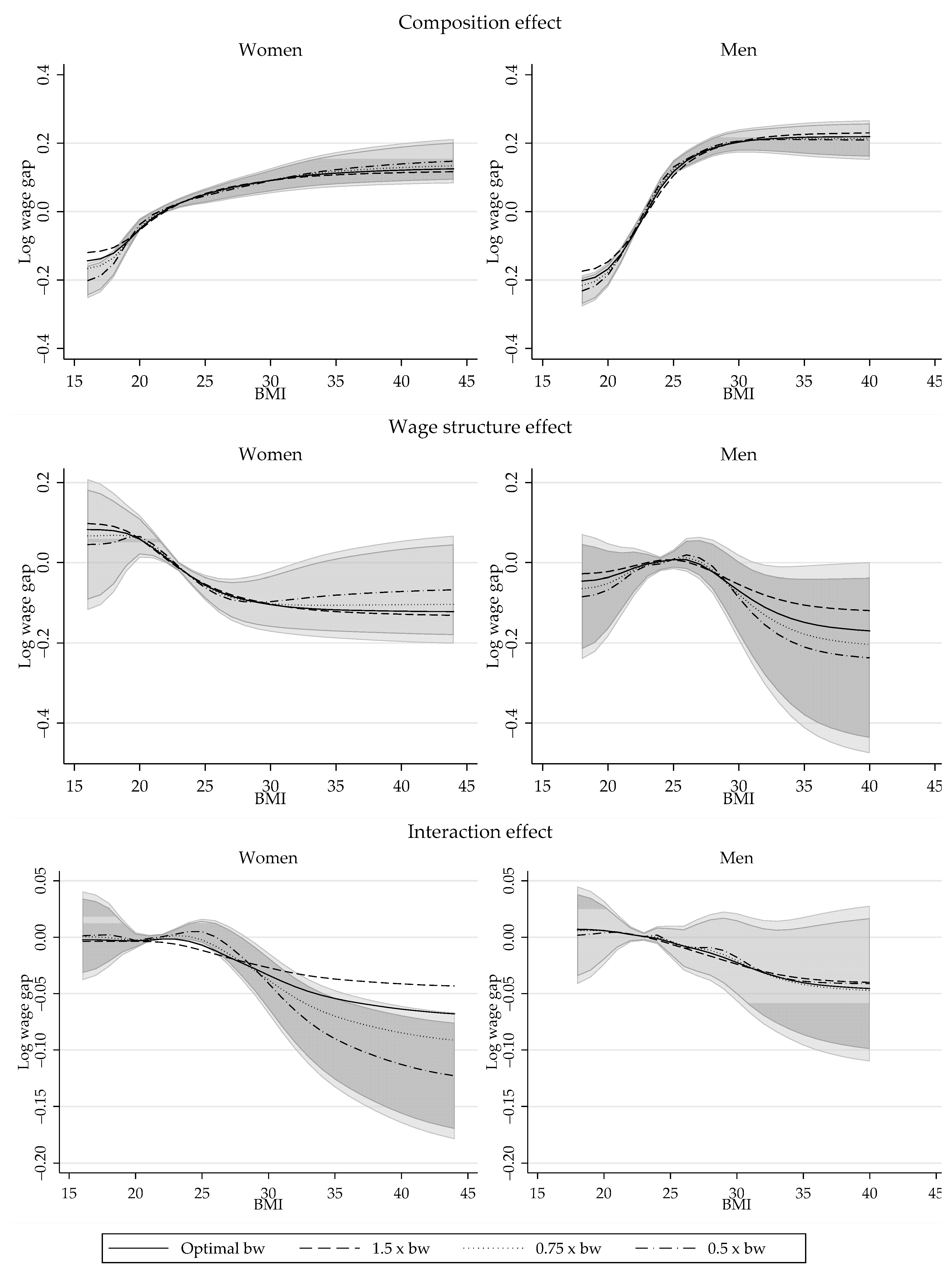
The bandwidth for the kernel regressions is selected separately for white men and white women using the cross-validation procedure described in Section 4.2, using the OLS-GIMR as the selection correction term. To reduce impact of sparse areas in the distribution of BMI on the bandwidth selection, two approaches were taken. The first is to set for observations at the top and bottom 1% of the distribution. The second is to use a strictly monotonic transformation of BMI, specifically the cumulative distribution G(BMI), as the grouping variable for the estimation of the local linear regressions.25 This transformation is similar to varying the bandwidth since more information will be used in areas that are more sparsely distributed than others, but it can also be compared to the use of k-nearest neighbors estimators. All models are estimated using Gaussian kernel functions. Table 4 provides the optimal bandwidths obtained from the cross-validation procedure for both men and women.26
6.2.2. Aggregate Decomposition Results
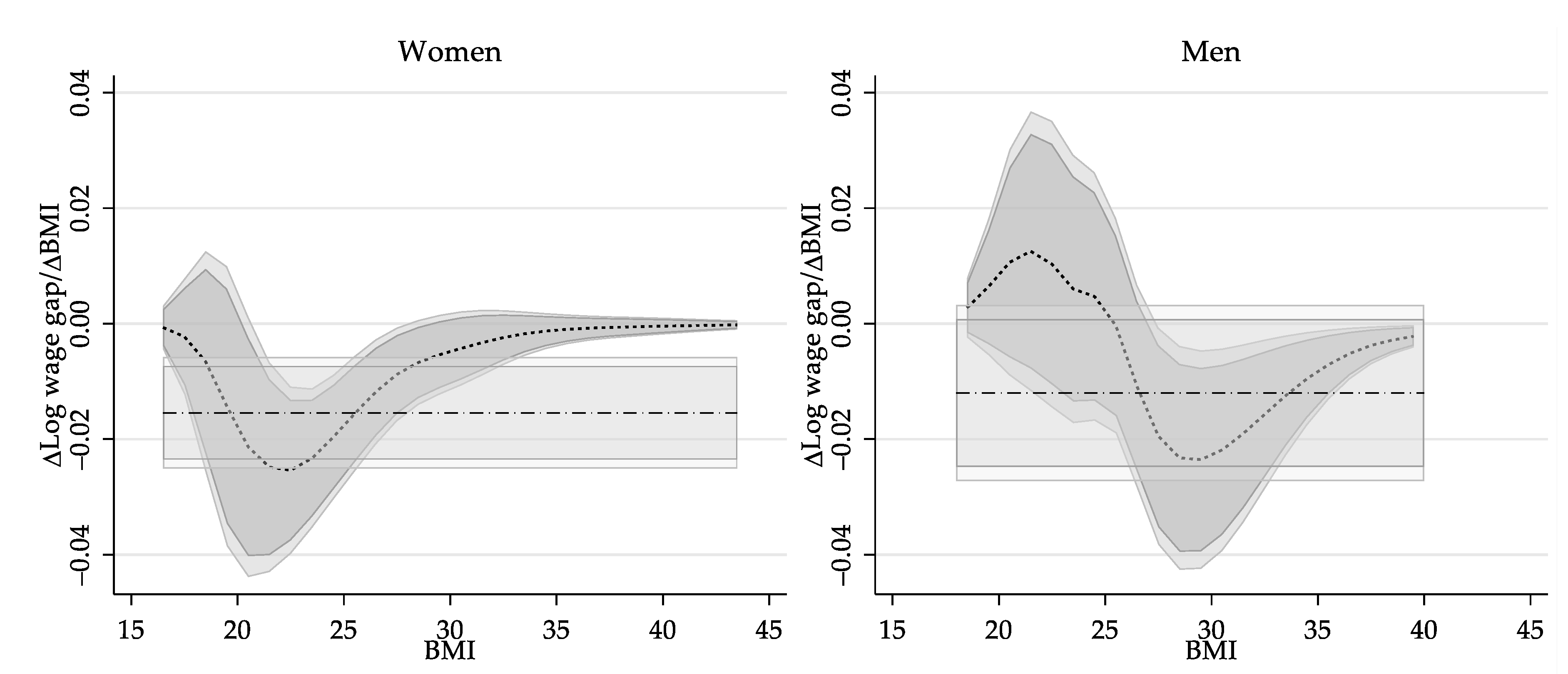
Figure 1 plots the selectivity corrected wage gap across the BMI for men and women, comparing people at all points of the BMI distribution with those in the reference group. The panels on the right provide the estimates that use the original BMI variable for the semiparametric regression, while the panels on the left show the estimates using the transformed variable G(BMI), but rescaled. The darker and lighter regions show the 90% and 95% confidence intervals constructed using a clustered paired bootstrap procedure with 399 repetitions. For men and women, the displayed gaps are provided for the relevant range of BMI which excludes the top and bottom 1% of the distribution.
According to the estimations, the selectivity corrected wage gap for men and women exhibit an inverse U shape with respect to their BMI. For women, I estimate a negative but non-statistically significant wage gap for all points of the BMI distribution. Based on the semiparametric estimation that relies on transformed BMI data, women at the top of the BMI distribution earn in average 6% less than the average women with healthy BMI, which is significant only at 10% level. The results based on kernel regressions with the original distribution of BMI provide qualitatively similar results but with lower precision at the extremes of the distribution.
In the case of men, the results suggest those with a BMI above 23 exhibit a positive and statistically significant wage gap compared to the reference group. The largest positive gap (16%) is observed for men with a BMI around 27, but this declines steadily for men with higher BMI, and turns statistically not significant for men with a BMI above 32. Men with a BMI below 22 show a negative wage gap, as large as 28% (based on the original variable distribution). Similar to the results for women, the estimates for men at the top of the BMI distribution are less precise when using the original BMI for the semiparametric regression. Because the results using the transformed variable are more precise than the alternative, the rest of the analysis will center on these estimations alone.27
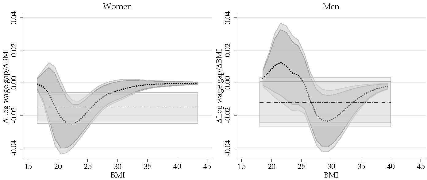
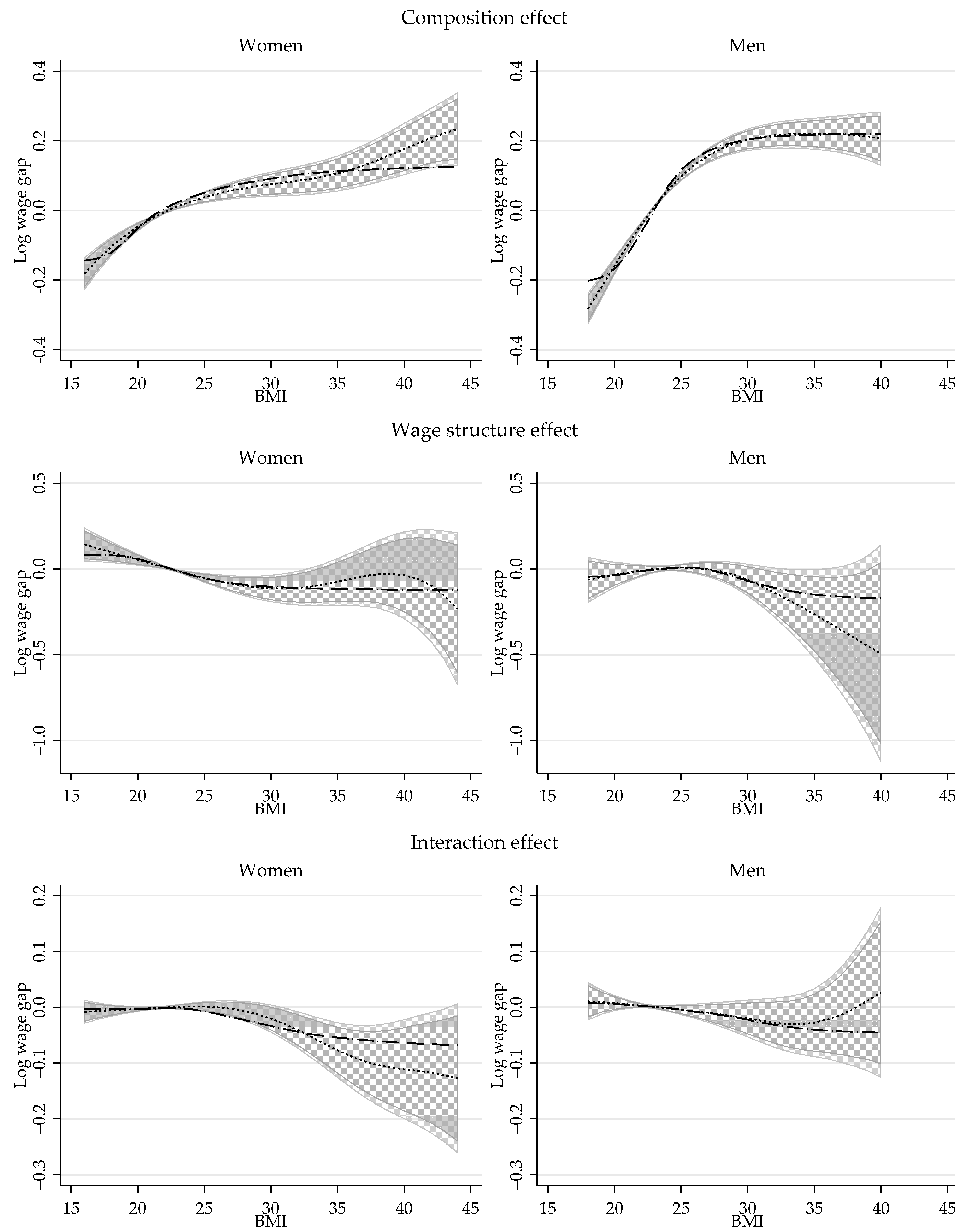
Similar to the standard OB analysis, the total wage gap reported in Figure 1 is not an adequate measure of the wage gap driven by differences in BMI because it is are driven by differences in characteristics (composition effect), coefficients (wage structure effect) or a combination of both. On Figure 2, I provide the semiparametric estimations for these three components for men and women.
According to the estimations, the composition effect has a large and statistically significant impact when explaining the wage gaps based on BMI. Its magnitude, which is larger for men than women, shows a monotonically increasing trend with respect to BMI, but at a decreasing rate. Across the distribution of BMI, differences in characteristics explain a wage gap that ranges between −20% to 21% for men, and −14% to 12% for women, when looking at people with BMI of 18 and 40, and compared to people with healthy BMI. This implies that white men and women with higher BMI have on average better endowments, which translates into higher wages.
Consistent with Cawley (2004) estimates, the wage structure effect for women shows a monotonically decreasing trend respect to BMI across the whole distribution, suggesting that BMI has a negative but non-linear impact on wages. The estimations show that there is a steady decline in the wage structure component among women, with a wage gap that goes from +8% for women with BMI of 18, to a wage gap of −11% for women with a BMI of 30.
For men, the effect of BMI on wages shows a different pattern. On the one hand, the results are less precise and the wage structure effect is not statistically significant across BMI. Setting aside the low precisions of the estimates, the wage structure effect for men shows an inverse u shape with respect to BMI. Compared to men with a BMI of 25, for whom a point estimate of +0.7% wage structure gap is estimated, the wage premium declines at lower and higher ends of BMI distribution. This may explain why the instrumental variable estimates for men’s (see Table 3) is negative but not statistically significant.
The last component of the decomposition is the interaction effect, which accounts for the fact that average wages are different because both coefficients and characteristics differ across groups. For men and women, the interaction effect grows negative with higher BMI, but it is only statistically significant for women.
6.2.3. Revisiting the Impact of Obesity on Wages: Partial Effect of BMI
One of the conclusions in Cawley (2004) is that a one standard deviation increase in body weight (roughly 32lbs), or equivalently a 5.5 BMI points increase, is associated with a drop in wages of 9%.28 This is a linear extrapolation of the estimates of their preferred model which suggest that a one-point increase in BMI is associated with a wage reduction of 1.7%.
While the results provided on Figure 2 cannot be directly compared to these findings, a modification of the wage structure effect in Equation (19) can be used to obtain partial effects that can be directly compared to Cawley’s results. Specifically, using characteristics fixed to the reference group, the marginal effect of BMI on the wage structure effect can be calculated as follows:
Figure 3 provides the estimations of the change of the wage structure effect as a function of BMI, and compares them to the marginal effect based on the replication of the IV linear estimates presented in Table 3.29
The marginal effect of BMI on the wage structure for women with a BMI between 20 and 25 is larger than that based on the linear IV estimate. The largest estimated marginal effect indicates that one-point increase in BMI for a woman with a BMI score of 22.5 relates to a wage decline of 2.5%, an almost 65 percent greater effect than linear IV estimate (1.5%). The negative impact of increasing BMI is not statistically significant for women with BMI below 20 or above 29, and the impact is below 0.5% for women with a BMI below 18 or above 30. Men with a BMI below 25 seem to experience a small positive wage gain associated with increasing BMI, although it is not statistically significant. The wage penalty due to a higher BMI is statistically significant above 27, with the largest wage decline is measured at 2.3% (at a BMI of 29.5), almost twice as large as the linear IV estimates of 1.2%. While the partial effect on wages decrease as BMI increases, it remains statistically significant through the rest of the BMI distribution.
7. Conclusions
In this paper, I have presented a methodology for the implementation of Oaxaca–Blinder decomposition when the grouping variable is continuous, and there is presence of endogenous selection into groups. This methodology uses a semiparametric approach known as varying coefficient models (Hastie and Tibshirani 1993), which has the advantage to provide a more flexible specification on the parameterization of the coefficients, compare to the models proposed by Ñopo (2008) and Ulrick (2012). Specifically, this paper describes the use of kernel local linear regressions for the estimation of such models.
The use of the generalized inverse mills ratios, also known as generalized residuals, allow for a feasible strategy to control for the endogenous selection based on the continuous grouping variable. This methodology is similar to the one proposed in Delgado et al. (2019), suggesting a similar control function approach to address endogeneity from the semiparametric component of the regression. While I do not discuss the theoretical properties of the estimator, the Monte-Carlo Simulation exercises suggests that the proposed strategy provides a simple but powerful approach to obtain consistent estimators of the outcome model parameters. This suggests that the proposed estimator can be used alongside to the methodologies proposed by Centorrino and Racine (2017) and Delgado et al. (2019). A more formal analysis of theoretical properties of the proposed estimator is left for future research.
This methodology may prove useful for the analysis of endogenous treatment effects with varying treatment intensity, when heterogeneous effects are present. In addition, it can also be used for analyzing the heterogeneity of the impact of other exogenous variables conditional on a grouping variable of interest.
In the illustration example, I revise the results from Cawley (2004) to evaluate the causal effect of BMI on wages. The application of the semiparametric OB decomposition shows that the association between BMI and wages is nonlinear, and that the negative impact of BMI on wages varies considerably compared to the effect described in Cawley (2004). Furthermore, it showed that for men, BMI also has a statistically significant and negative association with wages, which was not captured previously because of the weak but positive impact that BMI has on wages for men with low BMI.
Conflicts of Interest
The author declares no conflict of interest.
Appendix A. Additional Monte-Carlo Simulations
Setup: Centorrino and Racine (2017).
For this exercise, I follow the second scheme described in Centorrino and Racine (2017). In this setup, the variables of interest are defined as follows:
where represents a joint normal distribution, is the cumulative distribution function of a standard normal, and is the Bernoulli distribution with probability of success p.
The endogenous variable is defined as:
In this case, the endogenous variable d has a bounded distribution, which ranges from 0 to 1. and has a nonlinear relationship with the exogenous variables and the errors of the model. The smooth coefficients are defined as:
Finally, the outcome is defined as:
Table A1, Table A2 and Table A3 provides a summary of the Monte-Carlo Simulations using samples of size 1000, and 199 repetitions for the bootstrapped standard errors, using the three methodologies for the estimation of GIMR. Different from the simulation exercise in text, there are notable differences when using different GIMR. While all options show similar performance in terms of coverage, identifying the parameters and , OLS-GIMR performs the worse in correctly identifying the constant , with the estimates using OP-GIMR performing the best. The Bias corrected coverage suggests that the estimator has near to 95% of cases falling within the 95% confidence interval.

Table A1.
Monte-Carlo Simulations: OLS GIRM.
| True | Bias | 95% | 95% | |||
| Cov. | BC Cov. | |||||
| 0.05 | 0.005 | 0.019 | 0.057 | 0.055 | 93.8% | 94.4% |
| 0.15 | 0.045 | 0.019 | 0.057 | 0.056 | 93.5% | 93.9% |
| 0.25 | 0.125 | 0.019 | 0.059 | 0.056 | 94.2% | 93.7% |
| 0.35 | 0.245 | 0.019 | 0.059 | 0.057 | 93.8% | 93.8% |
| 0.45 | 0.405 | 0.020 | 0.059 | 0.057 | 93.5% | 93.8% |
| 0.55 | 0.605 | 0.019 | 0.059 | 0.058 | 94.8% | 94.7% |
| 0.65 | 0.845 | 0.019 | 0.059 | 0.058 | 94.4% | 95.0% |
| 0.75 | 1.125 | 0.020 | 0.059 | 0.057 | 93.2% | 94.5% |
| 0.85 | 1.445 | 0.020 | 0.059 | 0.057 | 93.5% | 94.1% |
| 0.95 | 1.805 | 0.019 | 0.057 | 0.056 | 93.2% | 94.4% |
| True | Bias | 95% | 95% | |||
| Cov. | BC Cov. | |||||
| 0.05 | 0.156 | 0.000 | 0.026 | 0.026 | 94.7% | 94.8% |
| 0.15 | 0.454 | 0.000 | 0.027 | 0.026 | 95.6% | 95.6% |
| 0.25 | 0.707 | 0.001 | 0.027 | 0.027 | 95.1% | 95.3% |
| 0.35 | 0.891 | 0.000 | 0.028 | 0.027 | 94.7% | 94.8% |
| 0.45 | 0.988 | 0.001 | 0.028 | 0.027 | 94.2% | 94.4% |
| 0.55 | 0.988 | 0.000 | 0.028 | 0.027 | 94.9% | 95.0% |
| 0.65 | 0.891 | 0.000 | 0.027 | 0.027 | 94.8% | 94.8% |
| 0.75 | 0.707 | 0.001 | 0.027 | 0.027 | 94.6% | 94.5% |
| 0.85 | 0.454 | 0.000 | 0.027 | 0.027 | 94.7% | 94.7% |
| 0.95 | 0.156 | 0.000 | 0.026 | 0.026 | 95.2% | 95.3% |
| True | Bias | 95% | 95% | |||
| Cov. | BC Cov. | |||||
| 0.05 | 1.902 | −0.177 | 0.047 | 0.046 | 1.5% | 94.6% |
| 0.15 | 1.721 | −0.256 | 0.044 | 0.043 | 0.0% | 94.7% |
| 0.25 | 1.558 | −0.214 | 0.041 | 0.040 | 0.0% | 94.1% |
| 0.35 | 1.409 | −0.139 | 0.039 | 0.038 | 4.3% | 93.7% |
| 0.45 | 1.275 | −0.053 | 0.036 | 0.036 | 68.6% | 94.0% |
| 0.55 | 1.154 | 0.039 | 0.034 | 0.034 | 77.7% | 94.3% |
| 0.65 | 1.044 | 0.126 | 0.033 | 0.033 | 4.1% | 94.1% |
| 0.75 | 0.945 | 0.200 | 0.033 | 0.033 | 0.0% | 93.9% |
| 0.85 | 0.855 | 0.244 | 0.033 | 0.033 | 0.0% | 94.3% |
| 0.95 | 0.773 | 0.164 | 0.033 | 0.034 | 0.2% | 95.2% |
Note: corresponds to the simulated standard errors. corresponds to the average bootstrapped standard errors. For each simulation, 199 repetitions are used to estimate bootstrapped standard errors. Coverage (Cov.) was evaluated as the proportion of the cases where the true value falls within the normal based confidence interval. The Bias corrected coverage (BC Cov.) was evaluated as the proportion of the cases where the true value falls within the normal based after correcting for the average bias.
Table A2.
Monte-Carlo Simulations: Oprobit GIRM.
| True | Bias | 95% | 95% | |||
| Cov. | BC Cov. | |||||
| 0.05 | 0.005 | −0.003 | 0.046 | 0.044 | 94.1% | 94.5% |
| 0.15 | 0.045 | −0.004 | 0.047 | 0.045 | 93.9% | 94.3% |
| 0.25 | 0.125 | −0.003 | 0.047 | 0.045 | 94.2% | 93.8% |
| 0.35 | 0.245 | −0.004 | 0.047 | 0.046 | 94.1% | 94.2% |
| 0.45 | 0.405 | −0.002 | 0.048 | 0.046 | 93.8% | 94.1% |
| 0.55 | 0.605 | −0.003 | 0.047 | 0.046 | 93.6% | 94.2% |
| 0.65 | 0.845 | −0.004 | 0.047 | 0.046 | 94.0% | 94.0% |
| 0.75 | 1.125 | −0.003 | 0.048 | 0.046 | 93.6% | 94.0% |
| 0.85 | 1.445 | −0.003 | 0.047 | 0.046 | 94.1% | 94.3% |
| 0.95 | 1.805 | −0.007 | 0.047 | 0.046 | 93.6% | 94.1% |
| True | Bias | 95% | 95% | |||
| Cov. | BC Cov. | |||||
| 0.05 | 0.156 | 0.000 | 0.022 | 0.022 | 95.5% | 95.5% |
| 0.15 | 0.454 | 0.001 | 0.022 | 0.022 | 95.2% | 95.2% |
| 0.25 | 0.707 | 0.003 | 0.022 | 0.022 | 95.5% | 94.9% |
| 0.35 | 0.891 | 0.004 | 0.022 | 0.023 | 94.9% | 95.2% |
| 0.45 | 0.988 | 0.005 | 0.023 | 0.023 | 94.8% | 95.2% |
| 0.55 | 0.988 | 0.004 | 0.022 | 0.023 | 94.8% | 95.6% |
| 0.65 | 0.891 | 0.003 | 0.023 | 0.023 | 94.8% | 94.9% |
| 0.75 | 0.707 | 0.003 | 0.022 | 0.023 | 94.8% | 95.3% |
| 0.85 | 0.454 | 0.002 | 0.022 | 0.023 | 94.3% | 94.4% |
| 0.95 | 0.156 | 0.000 | 0.022 | 0.023 | 96.0% | 96.0% |
| True | Bias | 95% | 95% | |||
| Cov. | BC Cov. | |||||
| 0.05 | 1.902 | 0.002 | 0.037 | 0.037 | 95.3% | 95.4% |
| 0.15 | 1.721 | 0.001 | 0.034 | 0.033 | 95.5% | 95.5% |
| 0.25 | 1.558 | 0.001 | 0.032 | 0.032 | 94.6% | 94.4% |
| 0.35 | 1.409 | 0.000 | 0.032 | 0.031 | 93.9% | 93.8% |
| 0.45 | 1.275 | 0.000 | 0.031 | 0.030 | 94.4% | 94.4% |
| 0.55 | 1.154 | 0.001 | 0.030 | 0.030 | 94.8% | 95.0% |
| 0.65 | 1.044 | 0.002 | 0.029 | 0.029 | 94.6% | 94.6% |
| 0.75 | 0.945 | 0.001 | 0.029 | 0.029 | 94.6% | 94.7% |
| 0.85 | 0.855 | 0.001 | 0.029 | 0.029 | 94.8% | 94.6% |
| 0.95 | 0.773 | 0.002 | 0.031 | 0.031 | 94.4% | 94.2% |
Note: corresponds to the simulated standard errors. corresponds to the average bootstrapped standard errors. For each simulation, 199 repetitions are used to estimate bootstrapped standard errors. Coverage (Cov.) was evaluated as the proportion of the cases where the true value falls within the normal based confidence interval. The Bias corrected coverage (BC Cov.) was evaluated as the proportion of the cases where the true value falls within the normal based after correcting for the average bias.
Table A3.
Monte-Carlo Simulations: Fprobit GIRM.
| True | Bias | 95% | 95% | |||
| Cov. | BC Cov. | |||||
| 0.05 | 0.005 | −0.002 | 0.048 | 0.047 | 94.3% | 94.4% |
| 0.15 | 0.045 | −0.001 | 0.049 | 0.047 | 94.3% | 94.4% |
| 0.25 | 0.125 | −0.001 | 0.050 | 0.048 | 94.6% | 94.3% |
| 0.35 | 0.245 | −0.002 | 0.050 | 0.048 | 93.8% | 93.7% |
| 0.45 | 0.405 | 0.000 | 0.051 | 0.049 | 94.1% | 94.0% |
| 0.55 | 0.605 | −0.002 | 0.050 | 0.050 | 95.7% | 95.5% |
| 0.65 | 0.845 | −0.002 | 0.051 | 0.050 | 94.3% | 94.0% |
| 0.75 | 1.125 | 0.000 | 0.052 | 0.051 | 94.2% | 94.2% |
| 0.85 | 1.445 | −0.001 | 0.052 | 0.051 | 94.6% | 94.9% |
| 0.95 | 1.805 | −0.002 | 0.053 | 0.051 | 94.2% | 94.5% |
| True | Bias | 95% | 95% | |||
| Cov. | BC Cov. | |||||
| 0.05 | 0.156 | 0.000 | 0.023 | 0.023 | 95.3% | 95.1% |
| 0.15 | 0.454 | −0.001 | 0.023 | 0.023 | 94.9% | 95.0% |
| 0.25 | 0.707 | 0.000 | 0.024 | 0.024 | 95.0% | 94.9% |
| 0.35 | 0.891 | 0.000 | 0.024 | 0.024 | 94.5% | 94.6% |
| 0.45 | 0.988 | 0.001 | 0.025 | 0.024 | 95.4% | 95.3% |
| 0.55 | 0.988 | 0.000 | 0.024 | 0.024 | 95.4% | 95.4% |
| 0.65 | 0.891 | 0.000 | 0.025 | 0.025 | 95.8% | 95.8% |
| 0.75 | 0.707 | 0.001 | 0.025 | 0.025 | 94.5% | 94.6% |
| 0.85 | 0.454 | −0.001 | 0.025 | 0.025 | 94.9% | 94.7% |
| 0.95 | 0.156 | −0.001 | 0.025 | 0.025 | 95.2% | 95.1% |
| True | Bias | 95% | 95% | |||
| Cov. | BC Cov. | |||||
| 0.05 | 1.902 | −0.073 | 0.042 | 0.039 | 54.5% | 93.7% |
| 0.15 | 1.721 | −0.037 | 0.038 | 0.034 | 78.9% | 92.4% |
| 0.25 | 1.558 | −0.012 | 0.036 | 0.032 | 90.3% | 90.9% |
| 0.35 | 1.409 | 0.006 | 0.035 | 0.031 | 89.5% | 90.0% |
| 0.45 | 1.275 | 0.022 | 0.035 | 0.030 | 84.2% | 91.3% |
| 0.55 | 1.154 | 0.039 | 0.034 | 0.030 | 71.0% | 90.6% |
| 0.65 | 1.044 | 0.054 | 0.034 | 0.030 | 53.1% | 91.4% |
| 0.75 | 0.945 | 0.067 | 0.034 | 0.029 | 37.9% | 90.9% |
| 0.85 | 0.855 | 0.082 | 0.034 | 0.030 | 22.6% | 90.4% |
| 0.95 | 0.773 | 0.084 | 0.034 | 0.031 | 24.2% | 93.1% |
Note: corresponds to the simulated standard errors. corresponds to the average bootstrapped standard errors. For each simulation, 199 repetitions are used to estimate bootstrapped standard errors. Coverage (Cov.) was evaluated as the proportion of the cases where the true value falls within the normal based confidence interval. The Bias corrected coverage (BC Cov.) was evaluated as the proportion of the cases where the true value falls within the normal based after correcting for the average bias.
Appendix B. Sensitivity to Model Specifications and Bandwidth. Illustration
| Replication of Cawley (2004) | ||||||
| White | Black | Hispanic | ||||
| Male | Female | Male | Female | Male | Female | |
| BMI | −0.0131 | −0.0168 * | −0.00258 | −0.00191 | −0.00914 | −0.0124 |
| [0.00831] | [0.00496] | [0.00678] | [0.00600] | [0.00731] | [0.0125] | |
| N | 13,355 | 10,800 | 6811 | 5651 | 4374 | 3035 |
| Pooling Black and Hispanic | ||||||
| White | NonWhite | |||||
| Male | Female | Male | Female | |||
| BMI | −0.0131 | −0.0168 * | −0.00369 | −0.00515 | ||
| [0.00831] | [0.00496] | [0.00508] | [0.00544] | |||
| N | 13,355 | 10,800 | 11,185 | 8686 | ||
| Excluding Sample Weights | ||||||
| White | NonWhite | |||||
| Male | Female | Male | Female | |||
| BMI | −0.0126 | −0.0149 * | −0.00241 | −0.00643 | ||
| [0.00789] | [0.00471] | [0.00472] | [0.00518] | |||
| N | 13,355 | 10,800 | 11,185 | 8686 | ||
| Dropping if Parents education is missing | ||||||
| White | NonWhite | |||||
| Male | Female | Male | Female | |||
| BMI | −0.0118 | −0.0147 * | −0.003 | −0.00634 | ||
| [0.00803] | [0.00480] | [0.00481] | [0.00518] | |||
| N | 12,393 | 10,195 | 10,465 | 8224 | ||
| Modifying model specification | ||||||
| White | NonWhite | |||||
| Male | Female | Male | Female | |||
| BMI | −0.0124 | −0.0155 * | −0.0048 | −0.00673 | ||
| [0.00805] | [0.00487] | [0.00492] | [0.00535] | |||
| N | 12,191 | 10,111 | 9854 | 7963 | ||
| Dropping Extreme BMI values (below 16 and above 60) | ||||||
| White | NonWhite | |||||
| Male | Female | Male | Female | |||
| BMI | −0.0127 | −0.0154 * | −0.00425 | −0.00735 | ||
| [0.00804] | [0.00493] | [0.00504] | [0.00545] | |||
| N | 12,184 | 10,101 | 9844 | 7958 | ||
Note. * p < 0.01. Clustered standard errors in parenthesis.
Figure A1.
Kernel Densities of BMI across race and sex.
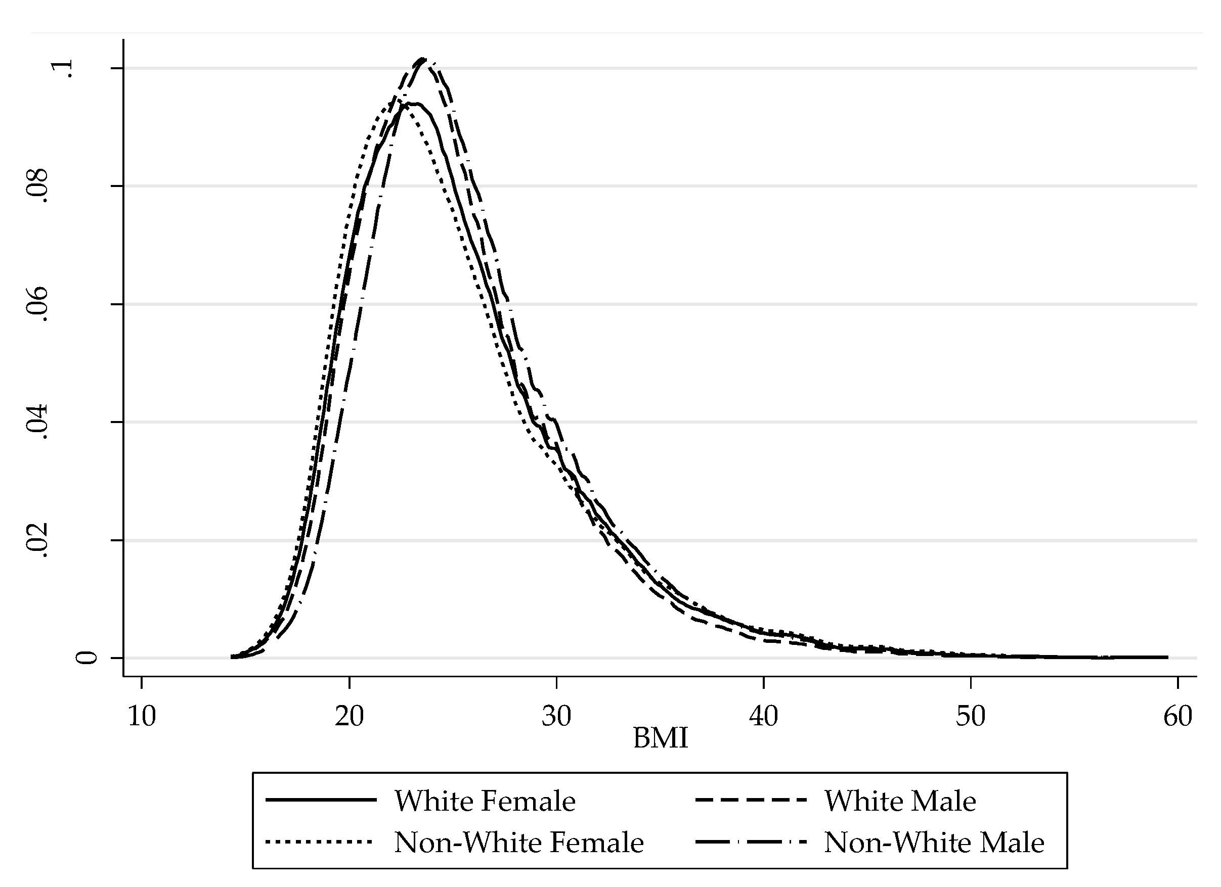
Figure A2.
Selectivity corrected Log wage gap by gender and GIMR estimation. Note: Shaded areas represent the 90% and 95% confidence interval based on bootstrapped standard errors, using OLS-GIMR.
Figure A2.
Selectivity corrected Log wage gap by gender and GIMR estimation. Note: Shaded areas represent the 90% and 95% confidence interval based on bootstrapped standard errors, using OLS-GIMR.

Figure A3.
Aggregate Semiparametric decomposition: OLS-GIMR. with kernel regression using BMI. Note: Dashed line is the estimation that uses G(BMI) for the kernel regression. Shaded areas represent the 90% and 95% confidence interval based on bootstrapped standard errors using BMI for the kernel regressions.

Figure A4.
Aggregate Semiparametric decomposition with kernel regression using G(BMI) Sensitivity to GIMR estimation method. Note: Shaded areas represent the 90% and 95% confidence interval, based on the bootstrapped standard errors for model using OLS-GIMR.
Figure A4.
Aggregate Semiparametric decomposition with kernel regression using G(BMI) Sensitivity to GIMR estimation method. Note: Shaded areas represent the 90% and 95% confidence interval, based on the bootstrapped standard errors for model using OLS-GIMR.
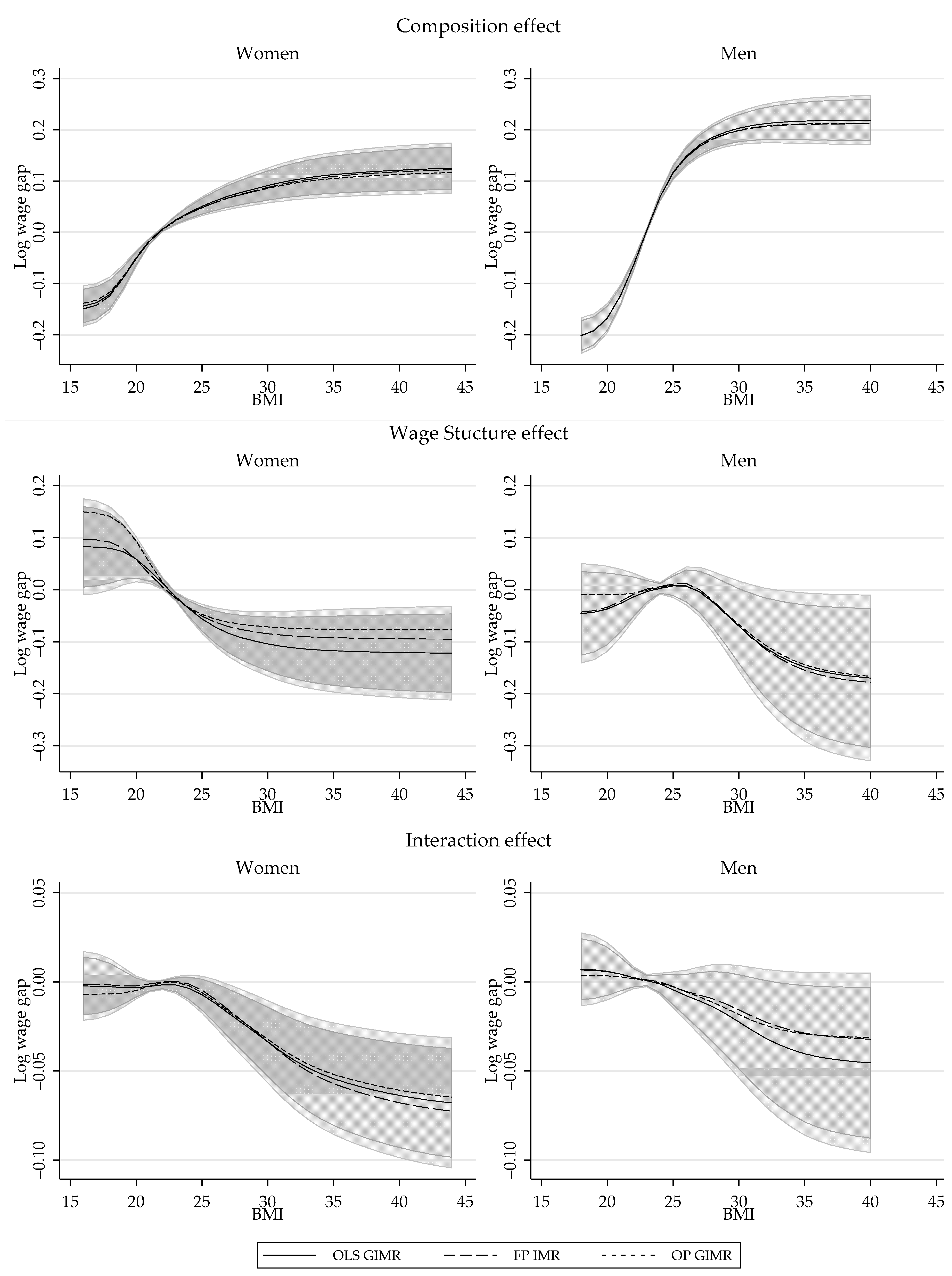
Figure A5.
Aggregate Semiparametric decomposition: Sensitivity to Bandwidth. OLS-GIMR. Note: Shaded areas represent the 90% and 95% confidence interval, based on the bootstrapped standard errors for model using OLS-GIMR, with a bandwidth half of the optimal.
Figure A5.
Aggregate Semiparametric decomposition: Sensitivity to Bandwidth. OLS-GIMR. Note: Shaded areas represent the 90% and 95% confidence interval, based on the bootstrapped standard errors for model using OLS-GIMR, with a bandwidth half of the optimal.

References
- Averett, Susan L. 2011. Labor market consequences: Employment, wages, disability, and absenteeism. In The Oxford Handbook of the Social Science of Obesity. Edited by J. Cawley. New York: Oxford University Press. [Google Scholar]
- Blinder, Alan S. 1973. Wage Discrimination: Reduced Form and Structural Estimates. The Journal of Human Resources 8: 436–55. [Google Scholar] [CrossRef]
- Cain, Glen G. 1986. The Economic Analysis of Labor Market Discrimination: A Survey. In Handbook of Labor Economics. Edited by Orley Ashenfelter and Richard Layard. Amsterdam: Elsevier Science Publishers, vol. 1. [Google Scholar]
- Cameron, A. Colin, and Pravin K. Trivedi. 2005. Microeconometrics: Methods and Applications. New York: Cambridge University Press. [Google Scholar]
- Cattaneo, Matias, and Michael Jansson. 2018. Kernel-based semiparametric estimators: Small bandwidth asymptotics and bootstrap consistency. Econometrica 86: 955–95. [Google Scholar] [CrossRef]
- Cawley, John. 2004. The Impact of Obesity on Wages. The Journal of Human Resources 39: 451–74. [Google Scholar] [CrossRef]
- Centorrino, Samuele, and Jeffrey S. Racine. 2017. Semiparametric Varying Coefficient Models with Endogenous Covariates. Annals of Economics and Statistics 128: 261–95. [Google Scholar] [CrossRef]
- Chernozhukov, Victor, Iván Fernández-Val, and Blaise Melly. 2013. Inference on Counterfactual Distributions. Econometrica Econometric Society 81: 2205–68. [Google Scholar] [CrossRef]
- Chiburis, Richard, and Michael Lokshin. 2007. Maximum likelihood and two-step estimation of an ordered-probit selection model. Stata Journal 7: 167–82. [Google Scholar] [CrossRef]
- Delgado, Michael S., Deniz Ozabaci, Yiguo Sun, and Subal C. Kumbhakar. 2019. Econometric Reviews, 1–23. [CrossRef]
- Fikkan, Janna L., and Esther D. Rothblum. 2012. Is fat a feminist issue? Exploring the gendered nature of weight bias. Sex Roles 66: 575–92. [Google Scholar] [CrossRef]
- Foresi, Silverio, and Franco Peracchi. 1995. The Conditional Distribution of Excess Returns: An Empirical Analysis. Journal of the American Statistical Association 90: 451–66. [Google Scholar] [CrossRef]
- Fortin, Nicole, Thomas Lemieux, and Sergio Firpo. 2011. Decomposition Methods in Economics. In Handbook of Labor Economics. Edited by Orley Ashenfelter and David Card. Amsterdam: Elsevier, vol. 4, Part A. pp. 1–102. [Google Scholar]
- Hastie, Trevor, and Robert Tibshirani. 1993. Varying-Coefficient Models. Journal of the Royal Statistical Society Series B (Methodological) 55: 757–96. [Google Scholar] [CrossRef]
- Heckman, James. J. 1979. Sample Selection Bias as a Specification Error. Econometrica 47: 53–161. [Google Scholar] [CrossRef]
- Henderson, Daniel J., and Christopher F. Parmeter. 2015. Applied Nonparametric Econometrics. Cambridge: Cambridge University Press. [Google Scholar]
- Horowitz, Joel. L., and Sokbae Lee. 2012. Uniform confidence bands for functions estimated nonparametrically with instrumental variables. Journal of Econometrics 168: 175–88. [Google Scholar] [CrossRef]
- Hotchkiss, Julie L., and Melinda M. Pitts. 2013. Even One Is Too Much: The Economic Consequences of Being a Smoker. Working Paper Series; WP 2013-3. Atlanta: Federal Reserve Bank of Atlanta. [Google Scholar]
- Keele, Luke J. 2008. Semiparametric Regression for the Social Sciences. New York: John Wiley & Sons. [Google Scholar]
- Kluve, Jochen, Hilmar Schneider, Arne Uhlendorff, and Zhong Zhao. 2012. Evaluating continuous training programmes by using the generalized propensity score. Journal of the Royal Statistical Society: Series A (Statistics in Society) 175: 587–617. [Google Scholar] [CrossRef]
- Lee, Lung-Fei. 1978. Unionism and Wage Rates: A Simultaneous Equations Model with Qualitative and Limited Dependent Variables. International Economic Review 19: 415–33. [Google Scholar] [CrossRef]
- Li, Qi, and Jeffrey. S. Racine. 2007. Nonparametric Econometrics: Theory and Practice. Woodstock: Princeton University Press. [Google Scholar]
- Ñopo, Hugo. 2008. An extension of the Blinder–Oaxaca decomposition to a continuum of reference groups. Economics Letters 100: 292–96. [Google Scholar] [CrossRef]
- Oaxaca, Ronald. 1973. Male-Female Wage Differentials in Urban Labor Markets. International Economic Review 14: 693–709. [Google Scholar] [CrossRef]
- Sabia, Joseph J., and Daniel I. Rees. 2012. Body weight and wages: Evidence from Add Health. Economics & Human Biology 10: 14–19. [Google Scholar]
- Terza, Joseph V. 1985. Ordered Probit: A Generalization. Communications in Statistics—A Theory and Methods 14: 1–11. [Google Scholar]
- Ulrick, Shawn W. 2012. The Oaxaca decomposition generalized to a continuous group variable. Economics Letters 115: 35–37. [Google Scholar] [CrossRef]
- Vella, Francis. 1998. Estimating Models with Sample Selection Bias: A Survey. The Journal of Human Resources 33: 127–69. [Google Scholar] [CrossRef]
- Williams, Richard. 2016. Understanding and interpreting generalized ordered logit models. The Journal of Mathematical Sociology 40: 7–20. [Google Scholar] [CrossRef]
- Wooldridge, Jeffrey. M. 2015. Control Function Methods in Applied Econometrics. Journal of Human Resources 50: 420–55. [Google Scholar] [CrossRef]
- Yatchew, Aonis. 2003. Semiparametric Regression for the Applied Econometrician. Cambridge: Cambridge University Press. [Google Scholar]
- Zhang, Wenyang, and Sik-Yum Lee. 2000. Variable bandwidth selection in varying-coefficient models. Journal of Multivariate Analysis 74: 116–34. [Google Scholar] [CrossRef]
| 1 | |
| 2 | This model is also known as smooth coefficient model. |
| 3 | Fortin et al. (2011) provide other scenarios where the conditional independence assumption might be violated. |
| 4 | |
| 5 | While identification of the Heckman selection model can be obtained based on the non-linearity alone, it is recommended to have an instrumental variable for better identification of the model. |
| 6 | For example, assuming counterfactual wages are given by the wage structure observed in Group B, the components of the decomposition would be given by , where can be interpreted as a treatment effect under the conditional independence assumption. |
| 7 | This model is also known as type-3 tobit models, or tobit selection models (Li and Racine 2007, sct. 10.3). |
| 8 | |
| 9 | This can be done, for example, using the kernel cumulative density estimation of . |
| 10 | Notice that does not vary with respect to the point of reference variable , but rather the individual realization . |
| 11 | Since we assume to be continuous, it should have no repeated values. In practice, due to intentional or unintentional measuring strategies continuous variables are available only in discrete form. This is the case for years of education in example used in Centorrino and Racine (2017). |
| 12 | See Cameron and Trivedi (2005), Chapter 9 for details on Kernel regression estimators. |
| 13 | Derivations of the bias and variance for kernel local linear estimators for varying coefficient models are provided in Section 9.3.2. in Li and Racine (2007). |
| 14 | See Section 9.3.2. in Li and Racine (2007) for further details. |
| 15 | This procedure is also followed in Centorrino and Racine (2017) for the construction of their confidence intervals. |
| 16 | Exploring the consequences of bandwidth selection within each bootstrap is beyond the scope of this paper. However, a simple exercise using Stata command npregress suggests that estimating the bandwidth for each bootstrap sample produces larger standard errors compared to using a fixed bandwidth. |
| 17 | Coverage estimates based on percentile confidence intervals show similar levels of coverage, and are not reported here. The simulation files are available upon request. |
| 18 | Appendix A provide additional simulations following the setups from Centorrino and Racine (2017), where d has a bounded distribution between 0 and 1. |
| 19 | |
| 20 | See Cawley (2004, p. 454) for a complete description of the data and model specification. |
| 21 | See Appendix B for complete set of results and intermediate steps for the data and model specification changes. |
| 22 | Control function approach using alternative measures for the GIMR were also estimated and are available upon request. While the results from the alternative specifications are similar to the ones presented here, they are somewhat larger and statistically significant for both white men and white women. |
| 23 | In scenarios like the analysis of wage penalties of smoking behavior, the reference group is clearly identified (non-smokers). In this case, one could argue that the assumption of smooth coefficients is only appropriate for people who smoke, and that coefficients for non-smokers should be estimated separately. |
| 24 | This scenario assumes that BMI has no additional impact on wages within the health group. Alternatively, following the critique raised by Cain (1986) in regards to using pooled data as the reference group, one could also include BMI as control in the pooled regression. For this illustration, such change has no substantial impact on the results. |
| 25 | In principle, this transformation should have no effect on the estimation of the semiparametric model. If , and is a strictly monotone transformation, then . |
| 26 | In practice, the bandwidth selection and estimation of the varying coefficient models are done using a set of commands written for the statistical software Stata. These programs are available upon request. |
| 27 | Figures in Appendix B provide various robustness checks including: Sensitivity to alternative GIMRs, results based on kernel regressions with original BMI distribution, and differences in the bandwidth estimation. |
| 28 | Cawley (2004, p. 465) stated that a two standard-deviation change in weight is associated with a 9 percent change in wages, when in fact this estimate reflects the impact of a one standard-deviation change in weight. |
| 29 | For internal consistency, the instrumental variable estimations include the quadratic terms and interactions as instruments. |
Figure 1.
Selectivity corrected Wage gap over BMI by gender. Note: Darker and lighter areas correspond to the 90% and 95% confidence intervals. Confidence intervals constructed based on bootstrapped standard errors with 399 repetitions clustered at the individual level.
Figure 1.
Selectivity corrected Wage gap over BMI by gender. Note: Darker and lighter areas correspond to the 90% and 95% confidence intervals. Confidence intervals constructed based on bootstrapped standard errors with 399 repetitions clustered at the individual level.

Figure 2.
Aggregated Semiparametric decomposition components. Note: Darker and lighter areas correspond to the 90% and 95% confidence intervals. Confidence intervals constructed based on bootstrapped standard errors with 399 repetitions clustered at the individual level.
Figure 2.
Aggregated Semiparametric decomposition components. Note: Darker and lighter areas correspond to the 90% and 95% confidence intervals. Confidence intervals constructed based on bootstrapped standard errors with 399 repetitions clustered at the individual level.

Figure 3.
Partial effect of BMI on the Wage Structure effect. Note: Darker and lighter areas correspond to the 90% and 95% confidence intervals for the linear IV estimate and the semiparametric estimate. Confidence intervals are constructed using the delta method and are based on Bootstrapped standard errors with 399 repetitions clustered at the individual level. The vertical axis measures the marginal effect of BMI on the wage structure component of the wage gap.

Table 1.
Monte-Carlo Simulation summary. Based on OLS-Generalized Inverse Mills Ratios.
| Sample 500 | Sample 1000 | Sample 2500 | ||||||||||||||
|---|---|---|---|---|---|---|---|---|---|---|---|---|---|---|---|---|
| True | 95% | 95% BC | 95% | 95% BC | 95% | 95% BC | ||||||||||
| Bias | Cov. | Cov. | Bias | Cov. | Cov. | Bias | Cov. | Cov. | ||||||||
| −3 | −0.600 | 0.178 | 0.326 | 0.299 | 87.0% | 92.6% | 0.110 | 0.232 | 0.223 | 90.3% | 94.2% | 0.056 | 0.157 | 0.154 | 92.4% | 94.6% |
| −2 | −0.393 | 0.145 | 0.224 | 0.205 | 86.4% | 91.9% | 0.096 | 0.159 | 0.152 | 88.4% | 94.3% | 0.052 | 0.107 | 0.105 | 91.7% | 95.8% |
| −1 | −0.119 | 0.130 | 0.185 | 0.178 | 88.2% | 93.0% | 0.094 | 0.139 | 0.132 | 86.0% | 93.7% | 0.059 | 0.094 | 0.090 | 88.7% | 93.7% |
| 0 | 0.363 | 0.007 | 0.185 | 0.182 | 95.2% | 95.4% | 0.005 | 0.135 | 0.134 | 95.4% | 95.4% | 0.004 | 0.093 | 0.092 | 94.5% | 94.5% |
| 1 | 0.798 | −0.143 | 0.218 | 0.204 | 85.4% | 93.0% | −0.113 | 0.158 | 0.152 | 86.8% | 94.0% | −0.077 | 0.106 | 0.104 | 85.2% | 94.1% |
| 2 | 0.763 | −0.050 | 0.243 | 0.238 | 93.0% | 93.6% | −0.025 | 0.174 | 0.179 | 96.2% | 95.7% | −0.007 | 0.126 | 0.124 | 95.3% | 95.5% |
| 3 | 0.681 | 0.009 | 0.292 | 0.285 | 95.2% | 94.7% | 0.028 | 0.206 | 0.218 | 96.6% | 96.1% | 0.032 | 0.156 | 0.151 | 94.2% | 94.6% |
| 4 | 0.807 | −0.065 | 0.391 | 0.357 | 91.7% | 92.8% | −0.020 | 0.278 | 0.274 | 94.3% | 94.5% | −0.002 | 0.202 | 0.191 | 94.3% | 94.3% |
| 5 | 1.000 | −0.144 | 0.528 | 0.494 | 90.8% | 92.3% | −0.075 | 0.384 | 0.371 | 92.8% | 93.5% | −0.041 | 0.258 | 0.258 | 94.4% | 95.3% |
| True | 95% | 95% BC | 95% | 95% BC | 95% | 95% BC | ||||||||||
| Bias | Cov. | Cov. | Bias | Cov. | Cov. | Bias | Cov. | Cov. | ||||||||
| −3 | 0.996 | −0.024 | 0.258 | 0.254 | 94.2% | 94.1% | −0.049 | 0.186 | 0.181 | 92.5% | 92.6% | −0.033 | 0.122 | 0.121 | 94.2% | 94.7% |
| −2 | 0.932 | −0.134 | 0.183 | 0.169 | 83.8% | 92.6% | −0.113 | 0.126 | 0.123 | 83.9% | 94.6% | −0.074 | 0.085 | 0.082 | 83.7% | 94.5% |
| −1 | 0.524 | −0.228 | 0.161 | 0.140 | 61.6% | 91.0% | −0.170 | 0.120 | 0.103 | 57.7% | 90.5% | −0.120 | 0.078 | 0.070 | 56.6% | 92.2% |
| 0 | −0.500 | −0.017 | 0.142 | 0.140 | 95.7% | 95.1% | −0.009 | 0.104 | 0.104 | 94.1% | 94.2% | −0.006 | 0.070 | 0.071 | 95.4% | 94.8% |
| 1 | −1.524 | 0.205 | 0.185 | 0.159 | 66.6% | 90.9% | 0.155 | 0.133 | 0.118 | 69.6% | 91.1% | 0.109 | 0.089 | 0.081 | 67.9% | 92.9% |
| 2 | −1.932 | 0.145 | 0.201 | 0.185 | 82.5% | 92.8% | 0.096 | 0.139 | 0.139 | 88.3% | 94.6% | 0.063 | 0.100 | 0.096 | 87.0% | 93.5% |
| 3 | −1.996 | 0.046 | 0.228 | 0.224 | 93.9% | 94.4% | 0.030 | 0.165 | 0.170 | 95.5% | 95.6% | 0.014 | 0.117 | 0.117 | 94.7% | 95.6% |
| 4 | −2.000 | 0.021 | 0.303 | 0.288 | 93.2% | 93.4% | 0.024 | 0.226 | 0.216 | 94.0% | 94.3% | 0.012 | 0.153 | 0.150 | 95.1% | 95.0% |
| 5 | −2.000 | 0.044 | 0.429 | 0.415 | 93.1% | 92.7% | 0.055 | 0.299 | 0.300 | 93.6% | 94.5% | 0.022 | 0.204 | 0.204 | 94.7% | 95.0% |
| True | 95% | 95% BC | 95% | 95% BC | 95% | 95% BC | ||||||||||
| Bias | Cov. | Cov. | Bias | Cov. | Cov. | Bias | Cov. | Cov. | ||||||||
| −3 | −0.800 | 0.427 | 0.758 | 0.684 | 85.3% | 92.5% | 0.274 | 0.557 | 0.534 | 89.7% | 93.7% | 0.127 | 0.384 | 0.376 | 92.3% | 93.7% |
| −2 | 0.000 | 0.224 | 0.406 | 0.390 | 91.0% | 94.1% | 0.143 | 0.306 | 0.292 | 90.7% | 93.4% | 0.072 | 0.214 | 0.203 | 93.0% | 93.3% |
| −1 | 0.600 | 0.089 | 0.260 | 0.250 | 92.8% | 94.5% | 0.049 | 0.187 | 0.184 | 94.3% | 94.2% | 0.021 | 0.126 | 0.125 | 94.1% | 94.5% |
| 0 | 1.000 | 0.012 | 0.175 | 0.166 | 93.4% | 93.4% | 0.000 | 0.125 | 0.121 | 93.6% | 93.6% | −0.009 | 0.081 | 0.082 | 95.4% | 95.3% |
| 1 | 1.200 | −0.027 | 0.140 | 0.136 | 93.7% | 94.6% | −0.023 | 0.105 | 0.101 | 93.4% | 94.1% | −0.015 | 0.069 | 0.068 | 94.2% | 94.4% |
| 2 | 1.200 | −0.024 | 0.222 | 0.219 | 94.5% | 94.5% | −0.030 | 0.164 | 0.165 | 94.9% | 95.2% | −0.019 | 0.113 | 0.112 | 94.9% | 94.7% |
| 3 | 1.000 | 0.024 | 0.406 | 0.398 | 94.7% | 95.1% | −0.009 | 0.294 | 0.306 | 95.8% | 95.6% | −0.019 | 0.218 | 0.210 | 94.6% | 94.6% |
| 4 | 0.600 | 0.107 | 0.713 | 0.670 | 92.3% | 93.4% | 0.037 | 0.538 | 0.525 | 94.0% | 94.6% | 0.007 | 0.390 | 0.370 | 93.4% | 93.6% |
| 5 | 0.000 | 0.279 | 1.233 | 1.134 | 91.9% | 94.1% | 0.168 | 0.946 | 0.892 | 91.5% | 92.3% | 0.083 | 0.632 | 0.634 | 94.7% | 94.8% |
Note: corresponds to the simulated standard errors. corresponds to the average bootstrapped standard errors. For each simulation, 199 repetitions are used to estimate bootstrapped standard errors. Coverage (Cov.) was evaluated as the proportion of the cases where the true value falls within the normal based confidence interval. The Bias corrected coverage (BC Cov.) was evaluated as the proportion of the cases where the true value falls within the normal based after correcting for the average bias.
Table 2.
Monte-Carlo Simulation summary: Alternative Generalized Inverse Mills Ratios estimates.
| Sample 5000 | OLS-GIMR | Oprobit-GIMR | Fprobit-GIMR | |||||||||||||
|---|---|---|---|---|---|---|---|---|---|---|---|---|---|---|---|---|
| Bias | 95% Cov. | 95% BC Cov. | Bias | 95% Cov. | 95% BC Cov. | Bias | 95% Cov. | 95% BC Cov. | ||||||||
| −3 | −0.600 | 0.035 | 0.117 | 0.114 | 92.6% | 93.8% | 0.035 | 0.117 | 0.114 | 92.7% | 93.9% | 0.034 | 0.117 | 0.114 | 92.6% | 93.8% |
| −2 | −0.393 | 0.027 | 0.081 | 0.079 | 93.0% | 93.8% | 0.026 | 0.081 | 0.079 | 93.1% | 93.8% | 0.026 | 0.081 | 0.079 | 93.4% | 93.9% |
| −1 | −0.119 | 0.041 | 0.068 | 0.067 | 90.5% | 94.5% | 0.041 | 0.068 | 0.067 | 90.7% | 94.4% | 0.040 | 0.068 | 0.067 | 90.8% | 94.5% |
| 0 | 0.363 | −0.002 | 0.069 | 0.068 | 94.5% | 94.8% | −0.002 | 0.069 | 0.069 | 94.5% | 94.8% | −0.002 | 0.069 | 0.069 | 94.3% | 94.8% |
| 1 | 0.798 | −0.063 | 0.082 | 0.078 | 86.0% | 94.1% | −0.062 | 0.082 | 0.078 | 86.3% | 94.0% | −0.061 | 0.083 | 0.078 | 86.2% | 94.0% |
| 2 | 0.763 | −0.006 | 0.095 | 0.092 | 93.6% | 93.7% | −0.006 | 0.096 | 0.093 | 93.6% | 93.6% | −0.006 | 0.096 | 0.093 | 93.7% | 93.5% |
| 3 | 0.681 | 0.022 | 0.122 | 0.113 | 93.0% | 92.9% | 0.022 | 0.122 | 0.113 | 93.0% | 92.8% | 0.022 | 0.123 | 0.114 | 93.1% | 92.6% |
| 4 | 0.807 | −0.005 | 0.144 | 0.144 | 94.7% | 94.6% | −0.005 | 0.144 | 0.144 | 94.7% | 94.7% | −0.005 | 0.145 | 0.145 | 95.0% | 94.7% |
| 5 | 1.000 | −0.024 | 0.202 | 0.193 | 93.0% | 92.7% | −0.024 | 0.202 | 0.193 | 92.9% | 93.1% | −0.023 | 0.203 | 0.194 | 92.9% | 93.1% |
| Bias | 95% Cov. | 95% BC Cov. | Bias | 95% Cov. | 95% BC Cov. | Bias | 95% Cov. | 95% BC Cov. | ||||||||
| −3 | 0.996 | −0.025 | 0.091 | 0.090 | 93.7% | 94.8% | −0.025 | 0.091 | 0.090 | 93.7% | 94.7% | −0.024 | 0.091 | 0.090 | 93.6% | 94.7% |
| −2 | 0.932 | −0.050 | 0.064 | 0.062 | 86.8% | 93.5% | −0.050 | 0.064 | 0.062 | 86.8% | 93.5% | −0.049 | 0.064 | 0.063 | 87.2% | 94.0% |
| −1 | 0.524 | −0.089 | 0.057 | 0.052 | 57.6% | 93.3% | −0.089 | 0.057 | 0.052 | 57.8% | 93.4% | −0.088 | 0.057 | 0.052 | 59.3% | 93.3% |
| 0 | −0.500 | −0.002 | 0.054 | 0.053 | 94.7% | 94.3% | −0.002 | 0.054 | 0.053 | 94.6% | 94.3% | −0.002 | 0.054 | 0.053 | 94.5% | 94.3% |
| 1 | −1.524 | 0.083 | 0.066 | 0.060 | 68.6% | 92.2% | 0.083 | 0.067 | 0.060 | 69.1% | 92.2% | 0.081 | 0.067 | 0.061 | 70.0% | 92.1% |
| 2 | −1.932 | 0.045 | 0.072 | 0.072 | 89.0% | 95.5% | 0.045 | 0.072 | 0.072 | 89.2% | 95.6% | 0.044 | 0.072 | 0.072 | 90.0% | 95.3% |
| 3 | −1.996 | 0.011 | 0.086 | 0.088 | 94.6% | 94.6% | 0.011 | 0.087 | 0.088 | 94.6% | 94.6% | 0.011 | 0.087 | 0.088 | 94.6% | 94.8% |
| 4 | −2.000 | 0.009 | 0.111 | 0.112 | 94.9% | 94.9% | 0.009 | 0.111 | 0.112 | 94.9% | 94.9% | 0.009 | 0.111 | 0.113 | 94.8% | 94.8% |
| 5 | −2.000 | 0.012 | 0.154 | 0.152 | 94.7% | 94.6% | 0.012 | 0.154 | 0.152 | 94.8% | 94.6% | 0.012 | 0.155 | 0.153 | 94.4% | 94.5% |
| Bias | 95% Cov. | 95% BC Cov. | Bias | 95% Cov. | 95% BC Cov. | Bias | 95% Cov. | 95% BC Cov. | ||||||||
| −3 | −0.800 | 0.082 | 0.287 | 0.282 | 93.7% | 93.9% | 0.081 | 0.288 | 0.282 | 93.8% | 93.9% | 0.079 | 0.288 | 0.283 | 93.8% | 94.1% |
| −2 | 0.000 | 0.034 | 0.158 | 0.152 | 93.0% | 93.5% | 0.033 | 0.159 | 0.152 | 93.1% | 93.1% | 0.032 | 0.159 | 0.153 | 93.5% | 93.6% |
| −1 | 0.600 | 0.011 | 0.090 | 0.092 | 95.4% | 95.1% | 0.011 | 0.090 | 0.092 | 95.4% | 95.1% | 0.010 | 0.091 | 0.093 | 95.2% | 95.1% |
| 0 | 1.000 | −0.009 | 0.061 | 0.060 | 94.8% | 94.8% | −0.009 | 0.061 | 0.060 | 94.9% | 94.6% | −0.009 | 0.061 | 0.061 | 94.8% | 94.7% |
| 1 | 1.200 | −0.018 | 0.050 | 0.050 | 94.2% | 95.4% | −0.018 | 0.050 | 0.050 | 94.2% | 95.3% | −0.018 | 0.050 | 0.051 | 94.3% | 95.5% |
| 2 | 1.200 | −0.016 | 0.086 | 0.083 | 93.3% | 93.3% | −0.016 | 0.086 | 0.083 | 93.3% | 93.2% | −0.016 | 0.086 | 0.083 | 93.4% | 93.3% |
| 3 | 1.000 | −0.007 | 0.162 | 0.157 | 93.8% | 93.9% | −0.007 | 0.163 | 0.157 | 93.9% | 93.8% | −0.007 | 0.164 | 0.158 | 94.1% | 93.7% |
| 4 | 0.600 | 0.018 | 0.280 | 0.277 | 94.1% | 94.3% | 0.017 | 0.280 | 0.278 | 94.2% | 94.2% | 0.017 | 0.281 | 0.279 | 94.3% | 94.2% |
| 5 | 0.000 | 0.045 | 0.496 | 0.478 | 93.9% | 94.0% | 0.044 | 0.497 | 0.479 | 93.8% | 93.9% | 0.042 | 0.499 | 0.481 | 93.6% | 94.1% |
Note. The Oprobit-GIMR was estimated using 50 groups of equal size. The Fprobit-GIMR was estimated using the empirical cumulative distribution of as dependent variable. For each simulation, 199 repetitions are used to estimate bootstrapped standard errors. Coverage (Cov.) was evaluated as the proportion of the cases where the true value falls within the normal based confidence interval. The Bias corrected coverage (BC Cov.) was evaluated as the proportion of the cases where the true value falls within the normal based after correcting for the average bias.
Table 3.
Replication, Modified Specification, and Control Function estimations.
| Replication of Cawley (2004) | ||||
| Ln (wage per h) | White | Nonwhite | ||
| Male | Female | Male | Female | |
| BMI | −0.0131 | −0.0168 * | −0.00369 | −0.00515 |
| [0.00831] | [0.00496] | [0.00508] | [0.00544] | |
| N | 13,355 | 10,800 | 11,185 | 8686 |
| Replication with changes in model specification and sample | ||||
| Ln (wage per h) | White | Nonwhite | ||
| Male | Female | Male | Female | |
| BMI | −0.0127 | −0.0154 * | −0.00425 | −0.00735 |
| [0.00804] | [0.00493] | [0.00504] | [0.00545] | |
| N | 12,184 | 10,101 | 9844 | 7958 |
| Control Function Approach: Instruments: Siblings BMI, age and sex | ||||
| Ln (wage per h) | White | |||
| Male | Female | |||
| BMI | −0.0127 | −0.0154 * | ||
| [0.00833] | [0.00527] | |||
| N | 12,184 | 10,101 | ||
| Instruments: Siblings BMI, age and sex, including interactions | ||||
| Ln (wage per h) | White | |||
| Male | Female | |||
| BMI | −0.012 | −0.0150 * | ||
| [0.00748] | [0.00530] | |||
| N | 12,184 | 10,101 | ||
Note: Clustered standard errors at the individual level in parenthesis. Control function approach estimates use bootstrapped standard errors clustered at the individual level with 250 repetitions. * p < 0.01.
Table 4.
Cross-validated Optimal Bandwidths.
| Variable of Reference | Men | CV Criterion | Women | CV Criterion |
|---|---|---|---|---|
| BMI | 3.2900 | −1.40814 | 4.8540 | −1.56378 |
| G(BMI) | 0.1769 | −1.40852 | 0.2241 | −1.54543 |
Note: CV = Cross-validation Log of Mean Squared leave-one-out error.
© 2019 by the author. Licensee MDPI, Basel, Switzerland. This article is an open access article distributed under the terms and conditions of the Creative Commons Attribution (CC BY) license (http://creativecommons.org/licenses/by/4.0/).
Share and Cite
MDPI and ACS Style
Rios-Avila, F. A Semi-Parametric Approach to the Oaxaca–Blinder Decomposition with Continuous Group Variable and Self-Selection. Econometrics 2019, 7, 28. https://0-doi-org.brum.beds.ac.uk/10.3390/econometrics7020028
AMA Style
Rios-Avila F. A Semi-Parametric Approach to the Oaxaca–Blinder Decomposition with Continuous Group Variable and Self-Selection. Econometrics. 2019; 7(2):28. https://0-doi-org.brum.beds.ac.uk/10.3390/econometrics7020028
Chicago/Turabian StyleRios-Avila, Fernando. 2019. "A Semi-Parametric Approach to the Oaxaca–Blinder Decomposition with Continuous Group Variable and Self-Selection" Econometrics 7, no. 2: 28. https://0-doi-org.brum.beds.ac.uk/10.3390/econometrics7020028
Note that from the first issue of 2016, this journal uses article numbers instead of page numbers. See further details here.