Evaluating Approximate Point Forecasting of Count Processes


1
Department of Mathematics and Statistics, Helmut Schmidt University, 22043 Hamburg, Germany
2
Sheldon B. Lubar School of Business, University of Wisconsin-Milwaukee, Milwaukee, WI 53211, USA
3
Institute of Mathematics, Department of Statistics, University of Würzburg, 97070 Würzburg, Germany
*
Author to whom correspondence should be addressed.
Econometrics 2019, 7(3), 30; https://0-doi-org.brum.beds.ac.uk/10.3390/econometrics7030030
Submission received: 1 April 2019
/
Revised: 21 June 2019
/
Accepted: 3 July 2019
/
Published: 6 July 2019
(This article belongs to the Special Issue Discrete-Valued Time Series: Modelling, Estimation and Forecasting)
Abstract
:In forecasting count processes, practitioners often ignore the discreteness of counts and compute forecasts based on Gaussian approximations instead. For both central and non-central point forecasts, and for various types of count processes, the performance of such approximate point forecasts is analyzed. The considered data-generating processes include different autoregressive schemes with varying model orders, count models with overdispersion or zero inflation, counts with a bounded range, and counts exhibiting trend or seasonality. We conclude that Gaussian forecast approximations should be avoided.
1. Introduction
Let be a count process and a count time series thereof, i.e., the are non-negative integer values from . After having fitted a model to the data available up to time T, in many applications, the aim is to predict the outcome of for some forecast horizon by computing a point forecast . When forecasting a real-valued process, the conditional mean is commonly used as a central point forecast, as this is known to be optimal in the sense of the mean squared error (MSE) (Box and Jenkins 1970; Gneiting 2011). Since count values are included in the set of real numbers, the same approach is commonly applied to count time series, despite the fact that the mean forecast will usually lead to a non-integer value. Actually, the discreteness of the count process is often ignored in practice, in the sense that a real-valued process model such as a Gaussian ARIMA model (Autoregressive Integrated Moving-Average, also Box–Jenkins model) is fitted to and then used for computing the required point forecasts. Forecasts of count processes are then approximated by taking either the rounded or ceiled value of the real-valued forecast. More recently, however, coherent forecasting techniques have been recommended (Bisaglia and Canale 2016; Freeland and McCabe 2004; Jung and Tremayne 2006; McCabe and Martin 2005; McCabe et al. 2011; Silva et al. 2009), which only produce forecasts in . This is achieved by computing the h-step-ahead conditional distribution of (given the past ) of the actual count process model, and by deriving an integer-valued quantity as the forecast value. The most widely used coherent central point forecast is the conditional median, which also satisfies an optimality property as it minimizes the mean absolute error (MAE) (Gneiting 2011). This paper is restricted to the conditional median if aiming at a central forecast, but the conditional mode might also be relevant in some applications (see Appendix D).
In certain applications, one is more interested in obtaining a non-central point forecast. In risk analysis, for example, when considering a loss distribution, particularly large outcomes of are viewed as an undesired event (e.g., large numbers of defects, large numbers of complaints, etc.) and, as such, viewed as a risk (Göb 2011). For a fixed risk level , one of the most common risk measures is the Value at Risk (), which is defined to be the th quantile of the (loss) distribution,
is interpreted as a threshold that is only exceeded in the worst cases. We use the obtained from the conditional distribution of , given the past , as a non-central (and coherent) point forecast. We refer to this type of as the “conditional ,” but we point out that it should not be confused with the risk measure of the same name1. Similar to the central median forecast, the conditional is either computed based on the actual count process model (thus leading to a coherent forecast), or in an approximate way by discretizing the conditional obtained from a real-valued process model.
Although there exist approaches of how to compute coherent point forecasts for count processes, these are often ignored in practice and methods for real-valued time series (plus discretization) are used instead. Thus, it is natural to ask how well these approximate forecasts perform compared to coherent forecasting techniques. There are only a few works in the literature that address this question. Quddus (2008) analyzed central point forecasts based on certain datasets about traffic accidents in Great Britain. It turned out that especially for the disaggregated datasets, a discrete forecasting model shows the best forecasting performance. Bisaglia and Gerolimetto (2015) performed a simulation study to compare the median forecast for a so-called Poi-INAR(1) process (see Appendix A for details) with the rounded-mean forecast, and they concluded that the Gaussian AR(1) approximation should be avoided. Alwan and Weiß (2017) considered quantile forecasts for INAR(1) processes in the context of demand prediction and showed that, in most cases, the approximate demand forecasts lead to severely increasing costs compared to coherent model-based forecasts. The simulation results presented by Maiti et al. (2016), who again compared Gaussian AR approximations to AR-like count processes, show a more mixed picture: while the approximation performed equally well with respect to (non-coherent) mean forecasts, it performed poorly concerning quantiles.
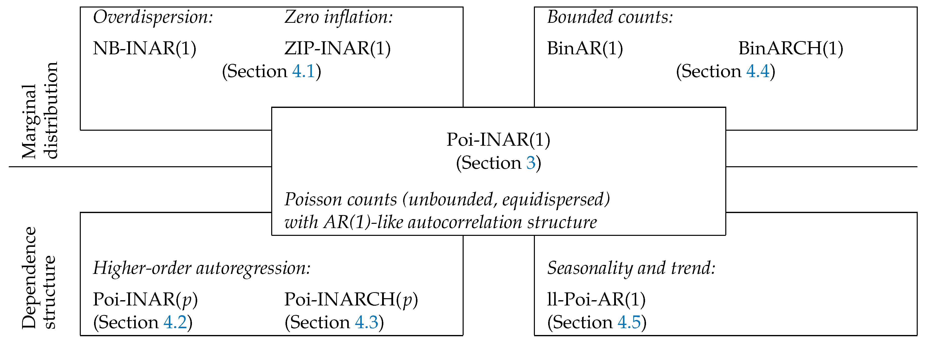
Although these works indicate that such discretized approximate point forecasts might perform quite poorly, it would be too premature to outright recommend against the approximate approach. Our reason for being cautious is the limited scope of the available works, which mainly focus on central forecasts for AR(1)-like Poisson counts. Therefore, we analyze the approximation quality of both central and non-central point forecasts in a comprehensive way by considering different types of data-generating process (DGP); see Appendix A for background information, various parameterizations of the respective models as well as different experimental designs. More precisely, we compute the conditional median as a central point forecast and the VaR as a non-central point forecast either in a coherent way by using the actual count process model, or in an approximate way by ignoring discreteness and working with a Gaussian time series model instead. In the latter case, the computed real-valued forecast is discretized by ceiling2 (i.e., mapping real numbers x to the least integer ), which corresponds to a Gaussian approximation without continuity correction (Homburg 2018). We investigate the quality of the approximate forecasts (either with or without estimation uncertainty) with respect to the performance metrics introduced in Section 2. Note that, in contrast to Bisaglia and Gerolimetto (2015); Maiti et al. (2016); Quddus (2008), we compute these forecast metrics precisely from the DGP’s model, not as data- or simulation-based empirical means (see Appendix A.4 for computational details). In Section 3, we start with a detailed analysis of the Poi-INAR(1) case, compare different experimental designs, and distinguish between approximation and estimation error in forecasting. We also consider the exponentially weighted moving-average (EWMA) forecasting method, which is quite popular among practitioners. In Section 4, we analyze the performance of the point forecasts for count processes with overdispersion or zero inflation, for higher-order autoregressions, for different types of AR-like models, for processes of bounded counts, and for non-stationary processes exhibiting trend or seasonality (see Figure 1 for an overview). Our analyses are illustrated with selected figures and tables; further results can be found at https://www.hsu-hh.de/mathstat/en/research/projects/forecastingrisk. Finally, we conclude in Section 5 and outline some issues for future research.
2. Evaluating the Performance of Coherent Point Forecasts
In this paper, we compare quantile-based coherent forecasts with their discretized counterparts obtained from a real-valued approximation of the actual count process. The performances of the approximate forecasts are evaluated based on selected inaccuracy measures, relative to the forecasts computed from the true count model. There are many proposals in the literature of how to evaluate the point forecasting inaccuracy (see Shcherbakov et al. 2013). Concerning central point forecasts, the Mean Absolute Error (MAE),
is commonly used (see Appendix A.4 for computational details), but also the Root Mean Squared Error (RMSE) is very popular (see Appendix C for the definition). While the RMSE is minimized by the conditional mean (which is not coherent for counts), the MAE is minimized by the conditional median (Gneiting 2011). Since we concentrate on the conditional median as the coherent central point forecast for counts in this work, we use the MAE as the appropriate performance measure. Nevertheless, in Appendix C, we also provide some background information on the use of MSE-based performance measures. The MAE is then used to define the following relative measure
where the subscript “f” refers to the forecasts to be evaluated (e.g., obtained from the approximating model by discretization, or by using estimated parameter values), and the subscript “t” represents the true count model of the DGP. Having, for example, an RMAE value of 1.5 implies that the MAE of the evaluated forecasting scheme is increased by 50% compared to the true model’s MAE, the latter being the unavoidable error in forecasting.
Concerning non-central point forecasts, inaccuracy measures are commonly based on asymmetric loss functions. The “lin-lin” loss function, for example, is given by
where the indicator function becomes 1 if A is true and 0 otherwise. Defining as the minimizer of the expectation thereof leads to the conditional -quantile, i.e., the is the optimal forecast with respect to this type of asymmetric loss (Christoffersen and Diebold 1997; Gneiting 2011). In a risk context, however, it seems to be more appropriate to only penalize exceedances (Lopez 1998). As such, we adjust the MAE to the situation of approximating a value in the right tail region and henceforth use the Mean Excess Loss (MEL) given by
as well as the corresponding relative measure
Again, we refer to Appendix A.4 for computational details, and to Appendix C for a brief discussion of the MSE’s tail version. The RMEL allows for a detailed insight into the inaccuracy of an approximate non-central point forecast. It takes the value 1 if the approximate forecast coincides with the true one. If the approximate forecast is larger than the true one, the RMEL takes a value . Then, we may interpret the forecast as being conservative, because in the practice of risk analysis, we would prepare for a larger risk than actually expected. In contrast, a RMEL value indicates that the actual risk is underrated, leading to an increased mean excess loss. In view of forecast accuracy, any deviation of the RMEL from 1 is undesirable, whereas, in practice, the costs associated with exceeding or falling below the true forecast might be different.
3. Baseline Model Poi-INAR(1): Approximate Forecasting and Performance Evaluation
As described in Section 1, our aim is to analyze the quality of different types of approximated point forecasts for count processes, where we evaluate their accuracy by the metrics introduced in Section 2. Our analyses are done in a comprehensive way by considering a wide variety of count process models (see Figure 1 for an overview). As a first step, in this section, we consider counts generated by a Poi-INAR(1) model, which constitutes an integer-valued counterpart to the Gaussian AR(1) model. The approximate point forecasts are derived from the Gaussian AR(1) model as described in Section 3.1. Their performance is first investigated without additional estimation uncertainty, to uncover the pure effect of approximation error; also different experimental designs are investigated in this context (see Section 3.2, Section 3.3 and Section 3.4). Section 3.5 focuses on the additional effect of estimation uncertainty.
3.1. INAR(1) Model and Gaussian Approximation
Let the true DGP be an INAR(1) process with . It is defined by the recursion , where the binomial thinning operator “∘” is used as a discrete-valued substitute of the conventional multiplication; see Appendix A.2 for further details about the nature of the process along with how h-step-ahead forecasts are computed.
Assuming that the Gaussian model is a good enough capture of the correlative structure, practitioners often ignore the discreteness of DGP’s range and approximate the DGP’s true model by a corresponding Gaussian model. In the INAR(1) case considered here, an approximating Gaussian AR(1) process would be used, which follows the recursion
where “i.i.d.” abbreviates “independent and identically distributed.” Here and throughout this article, we use and to denote the mean and variance, respectively, with the subscript indicating the considered random variable. For a Gaussian AR(1) process to be stationary, the requirement is . However, since we use it for approximating an INAR(1) process that only allows for positive autocorrelation3, we restrict to . In choosing the parameters of the Gaussian approximation, we distinguish between two scenarios:
- If the DGP’s parameterization is assumed to be known, we implement the Gaussian approximation according to the “X-method” considered by Homburg (2018), which calls for setting and , and the Gaussian variance is chosen such that (see Appendix B for details).
- If the DGP’s parameterization is assumed to be unknown, we directly fit the Gaussian approximate model to the given count time series. Then, we use the scenario with estimated parameters to consider the joint effect of approximation and estimation error.
After specification of the approximating Gaussian AR(1) process, the resulting approximate h-step-ahead forecast distribution is normal,
We obtain the approximate discrete point forecasts by first computing the corresponding real-valued forecast from Equation (7) (setting ), and by discretizing it afterwards. In this work, as explained in Section 1, we use the ceiling operation for discretization, which corresponds to the Gaussian approximation without continuity correction.
3.2. Evaluating Poi-INAR(1) Forecast Approximations
In this section, we consider the DGP Poi-INAR(1) (see Appendix A.2 for details). Using Equation (7) along with the “X-method,” the approximating forecast distribution is
with . To first analyze the influence of the distribution parameters and , we concentrate on the forecasting scenario, where the last observation is assumed to equal the median of the marginal distribution, and where the forecast horizon h equals 1. The influence of these two design parameters is examined in Section 3.3 and Section 3.4.
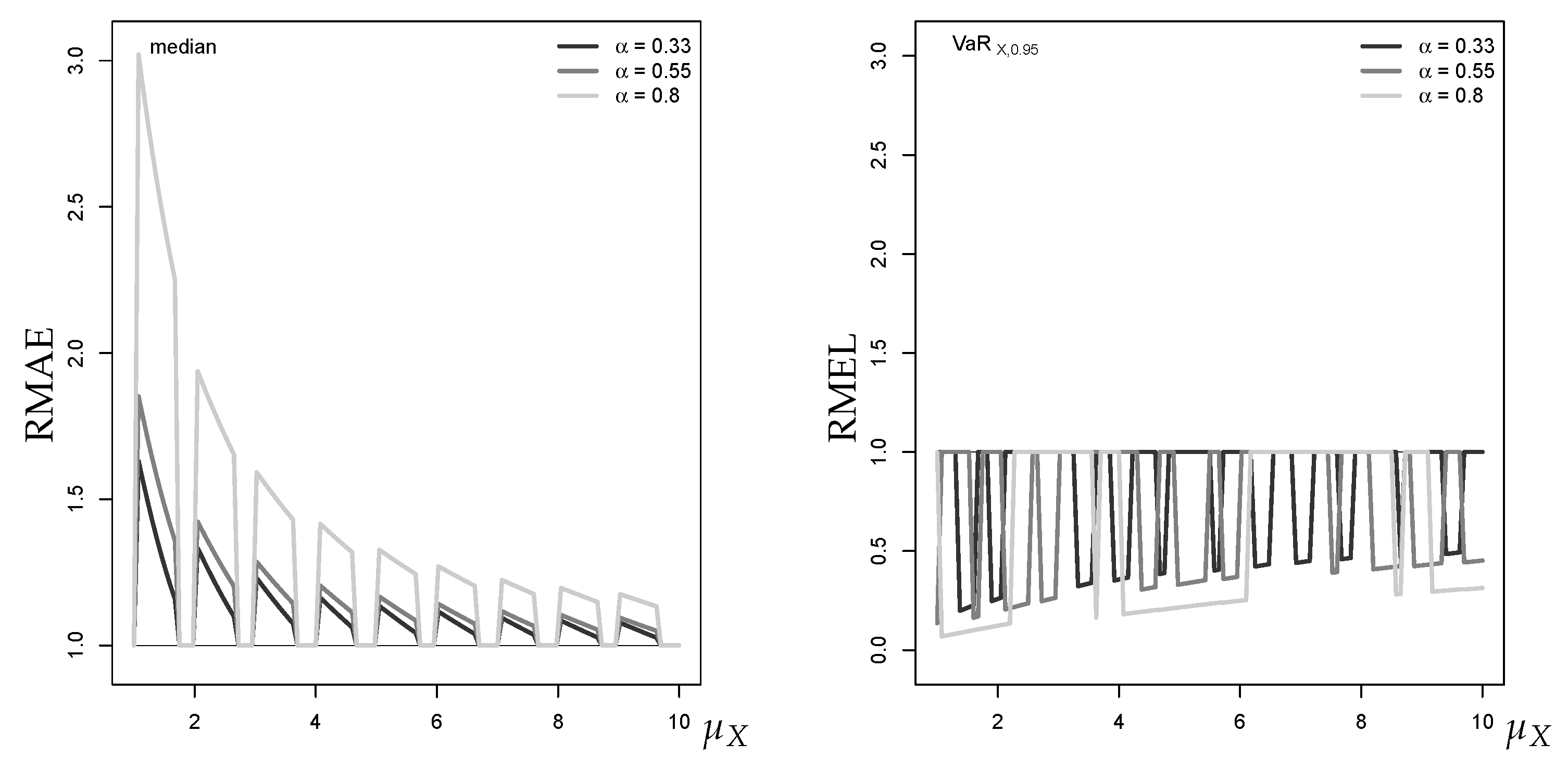
As a coherent central point forecast, we use the median of the discrete conditional distribution (see Section 1) as it expresses the center of the distribution in a probabilistic sense. By contrast, the approximate median is the ceiled Gaussian median. For different autocorrelation levels , the left graph in Figure 2 shows the computed RMAE values plotted against increasing mean . It can be seen that the RMAE tends towards 1 with increasing , i.e., the Gaussian approximation improves with increasing mean. This is plausible, because the Poisson distribution becomes less skewed with increasing and approaches normality because of the central limit theorem (Jolliffe 1995). Interestingly, for a given mean level, the RMAE increases with the autocorrelation parameter . Additionally, the gaps between RMAE values for different autocorrelation levels decrease with the mean level. For a typical low-count scenario with, say, and , we have to expect RMAE values between 1.5 and 3.0, and these values remain notably larger than 1 even for .
As already mentioned, we consider an upper quantile (VaR) as the coherent non-central point forecast. To evaluate the forecast performance of the approximate discrete upper quantile (ceiled Gaussian VaR), we use the RMEL defined in Section 2. The right graph in Figure 2 shows the RMEL values for the VaR approximation at level 95%. First, we note that the RMEL mainly takes values . This implies that the Gaussian approximation tends to exceed the true (conservative risk forecast). Furthermore, the RMEL tends very slowly towards 1 with increasing , thus the approximation quality improves much more slowly than for the central median forecast.
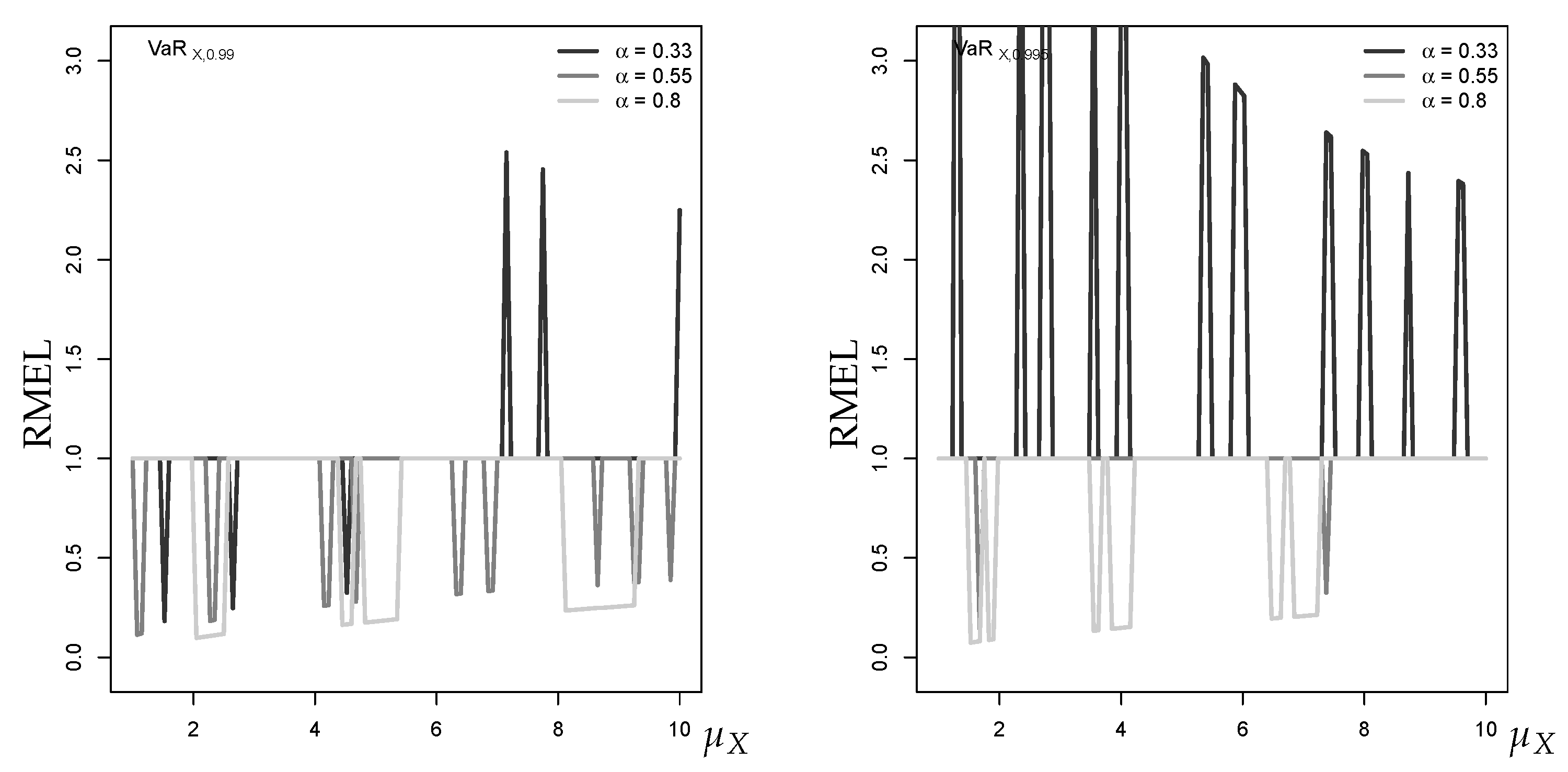
Figure 3 shows the RMEL for the higher quantile levels 99% and 99.5%. Again, it can be seen that the approximation improves in accuracy with increasing , but now the RMEL values are more often (underrating of the risk). Given the upper tail of the true forecast distribution (a Poisson-binomial mixture) is generally heavier than the corresponding tail of the normal distribution, this effect becomes particularly visible for very large quantile levels such as .
3.3. Effect of Last Observation
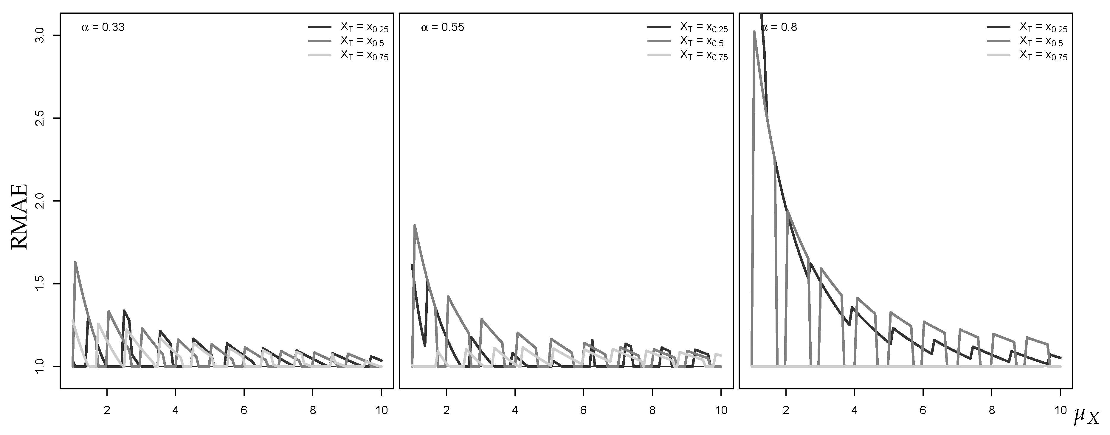
In the preceding analysis, the last observation is assumed to be the median of the true marginal distribution. Now, we analyze the effect of the location of . In Figure 4 and Figure 5, is set equal to the 50%-, 50%-, and 75%-quantile of the INAR(1)’s Poisson marginal distribution.
Generally, the accuracy of the median approximation of the one-step-ahead forecast distribution improves over . However, with increasing , the location of has a stronger effect on the actual RMAE level. While for located in the right tail region, the RMAE for fixed improves with increasing autocorrelation, it deteriorates for increasing if is located central or in the left tail region. For the approximation of the one-step-ahead forecast distribution, the location of appears to not have such a large influence on the accuracy of the Gaussian AR(1) approximation. Independent of the location of , we generally have RMEL values throughout .
Remark 1.
At this point, let us briefly comment on another scheme for VaR forecasting, as it is popular among financial practitioners: the historical simulation (HS) approach (see, e.g., Hendricks (1996)). The HS approach is a moving-window approach that computes the sample quantile from past observations (commonly, stock or portfolio returns) to generate a VaR forecast. If computing a sample quantile from a stationary process, it constitutes an estimate of the marginal distribution’s VaR. For forecasting, however, the conditional distribution’s VaR is more relevant. These alternative estimates of VaR can differ considerably for the autocorrelated count processes considered in the present work. Consider the example of a Poi-INAR(1) DGP with marginal mean , which has the marginal distribution and thus the marginal . The conditional VaRs depend on both the autocorrelation parameter α and the last observation , where the latter is chosen as either the 50%-quantile , the 50%-quantile , or the 75%-quantile :
- If , then leads to , to , and to .
- If , then leads to , to , and to .
- If , then leads to , to , and to .
As can be seen, the conditional VaRs vary considerably depending on the level of autocorrelation α and value of the last observation . Thus, in the context of our work on autocorrelated processes, the HS approach does not serve as a viable alternative for VaR estimation.
3.4. Effect of Forecast Horizon h
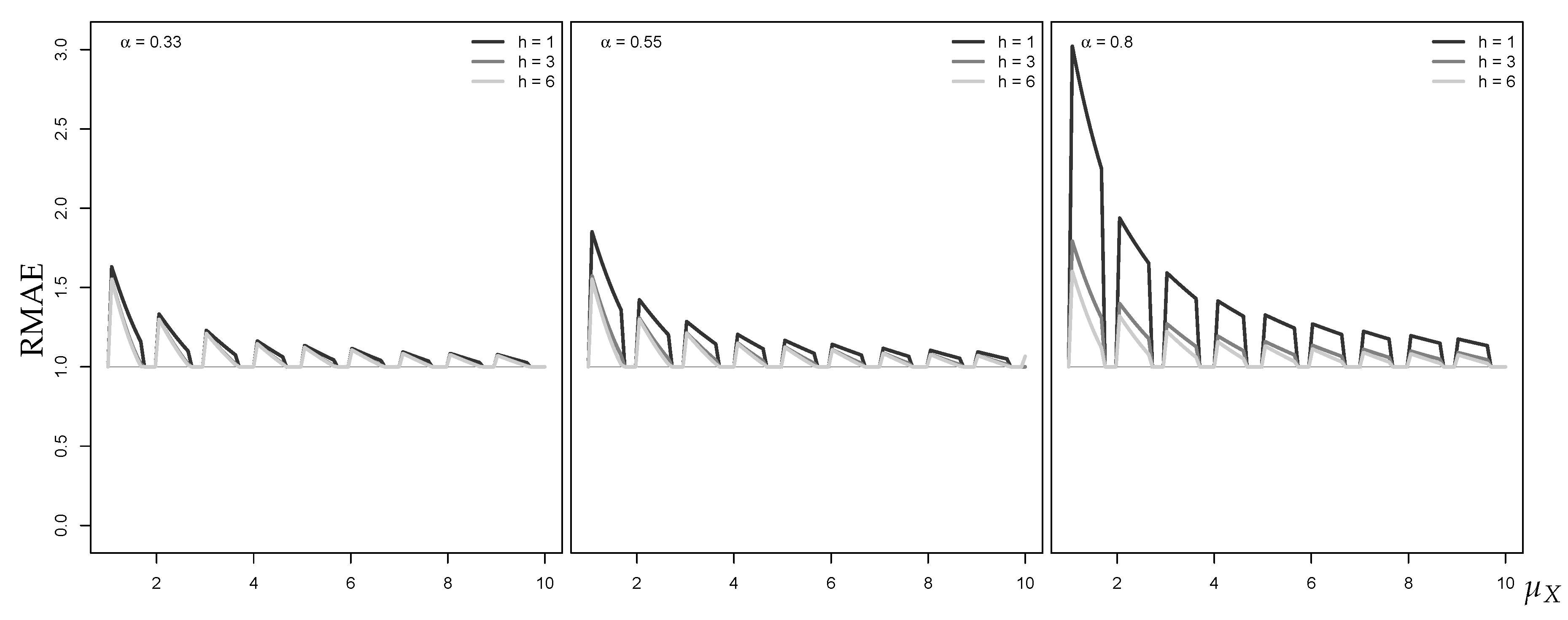
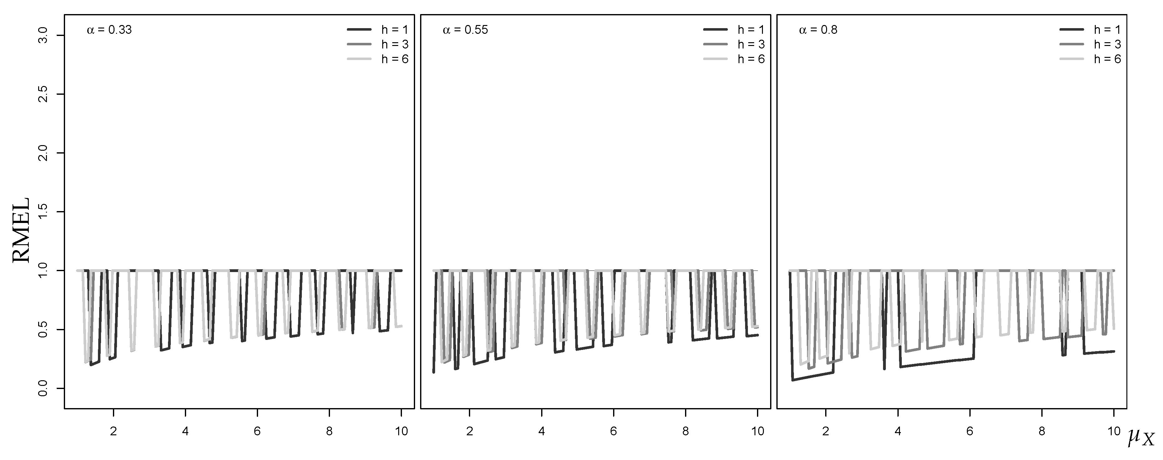
Let us now study the effect of an increasing forecast horizon h, causing the conditional forecast distribution to approach the stationary marginal distribution. For a given level of autocorrelation, Figure 6 shows that the h-step-ahead median approximation improves as h increases. Furthermore, it can be seen that performance deteriorates with increasing autocorrelation. As such, by concentrating on as in the previous sections, we obtain some kind of worst-case performance of the central Gaussian AR(1) approximation. Figure 7, in contrast, shows that an increased forecast horizon does not have a strong effect on the approximation of the h-step-ahead . Thus, the result for is representative for the overall performance of the non-central Gaussian AR(1) approximation.
3.5. Point Forecasts of Poi-INAR(1) Processes under Estimation Uncertainty
In Section 3.2, the performance of the (non-)central one-step-ahead point forecasts is evaluated for the case where model parameters are known. By doing so, we can explore the pure effect of the approximation error. In practice, however, the process parameters are usually not known and have to be estimated. Consequently, the point forecasts are also affected by estimation error. For the analyses presented in this section, we simulated 1000 Poi-INAR(1) time series per scenario. For each time series, the required model parameters (either for the Poi-INAR(1) fit or the Gaussian AR(1) fit) were estimated, and the forecasts were computed based on the fitted models. For parameter estimation, we used the method of moments (Yule–Walker estimation) because of computational efficiency. In practice, maximum likelihood estimation (MLE) is preferred due to better statistical properties than method-of-moments estimation (for the INAR family, forecasting based on non-parametric MLE would also be possible (see McCabe et al. 2011)). We experimented with MLE and found that it rarely had any observable effect relative to method-of-moments estimation; presumably, any advantages from MLE were lost with the discretizing of the forecasts. For each simulated time series and corresponding point forecast, the RMAE and RMEL values were computed, where deviations from 1 were now caused by either estimation error only (for the coherent forecasts from the fitted count model), or by both estimation and approximation error (for the forecasts from the fitted approximating model). The plotted points in the subsequent figures represent truncated means of these 1000 simulated RMAE and RMEL values; specifically, the 10 smallest and largest RMAE and RMEL values were truncated per simulation scenario to eliminate extreme values (outliers) from this calculation.
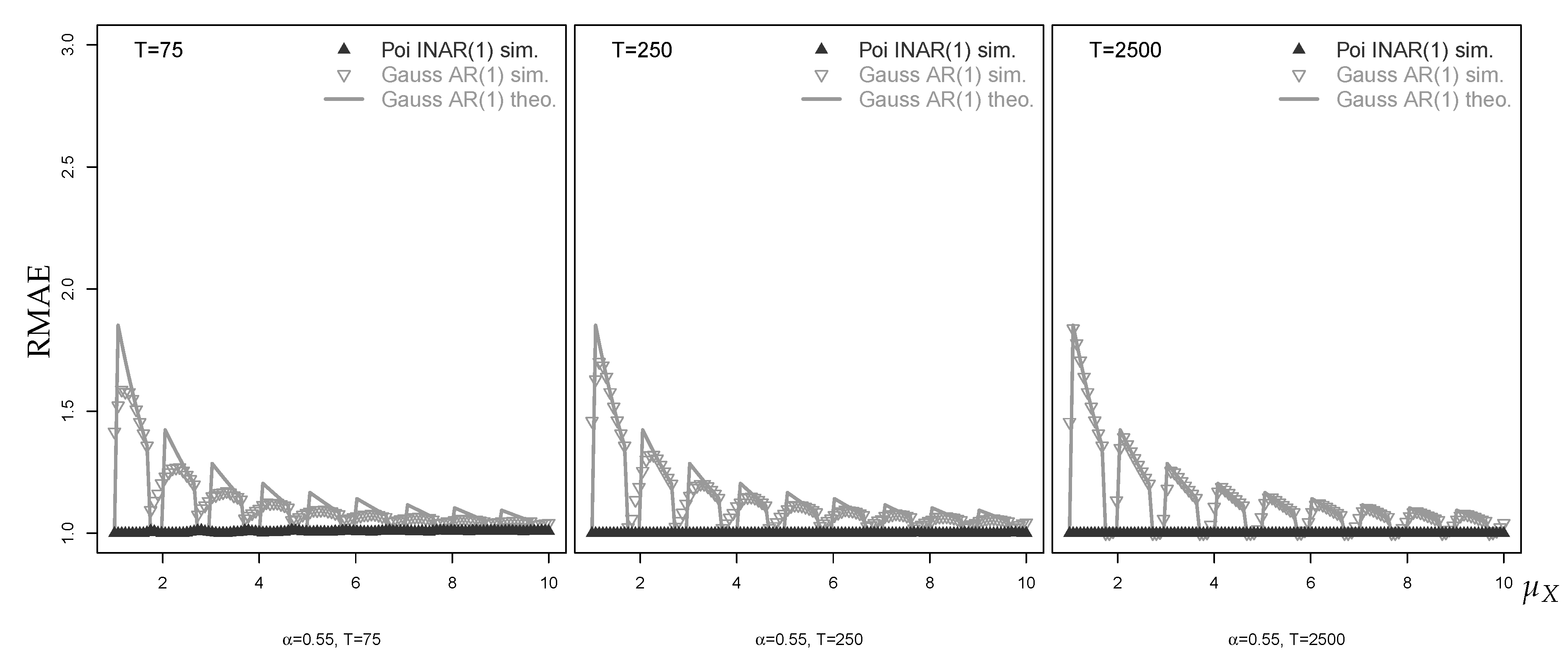
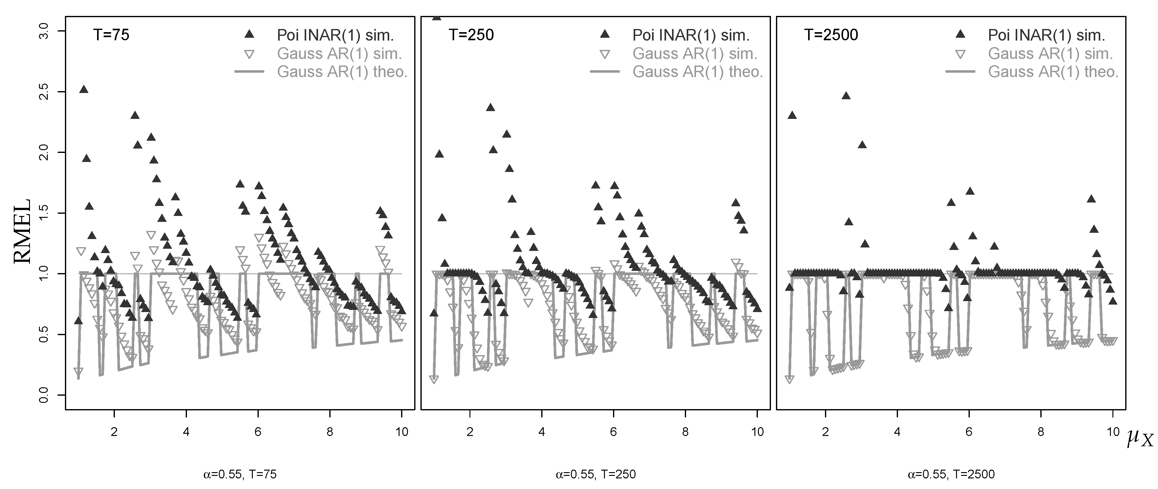
The means of the simulated RMAE and RMEL values (where is fixed as the median of the true marginal distribution) are shown as dots in Figure 8 and Figure 9, whereas the solid lines correspond to the respective curves for the known-parameter case in Figure 2.
The simulated RMAEs shown in Figure 8 demonstrate that the median forecasts based on the fitted Poi-INAR(1) model are only slightly affected by estimation error. Estimation error has a greater effect on the Gaussian approximate forecasts than on the Poi-INAR(1) forecasts. With this said, the RMAEs show a similar behavior against as the RMAEs for the known-parameter case. The situation becomes much more complicated for the -forecasts analyzed in Figure 9. Because of estimation error, both the Poi-INAR(1) forecasts and the Gaussian AR(1) forecasts may lead to RMEL values that deviate considerably from 1. Generally, with increasing sample size, the plotted points tend to settle down to the known-parameter counterparts. Interestingly, the Gaussian forecasts seem to settle down more generally with increasing T than it is the case with the Poi-INAR(1) forecasts, as can be seen with . Comparing Figure 8 and Figure 9, it is clear that the performance of central forecasts (of either type) is rather robust while non-central forecasts (of either type) are severely affected by estimation error.
Rather than using a fixed , we now consider the use of the last observation from each simulated time series as the starting point for forecasting. Figure 10 shows the resulting mean RMAE values for the median forecasts (left) and the mean RMEL values for the -forecasts (right) for the example situation . The RMAE values resulting from the fitted Poi-INAR(1) and Gaussian AR(1) model behave similarly as in Figure 8. In particular, the RMAE values corresponding to the Gaussian approximation converge towards 1 with increasing but show large deviations for small . In the RMAE graph, we also added another forecasting competitor: namely, the rounded EWMA forecast (with smoothing parameter chosen to minimize the squared one-step prediction error), which is often used by practitioners. Even though the EWMA forecasting method is always worse than the fitted Poi-INAR(1) model, it outperforms the Gaussian AR(1) forecast for . This effect amplifies with increasing autocorrelation. For example, for , the EWMA approximation provides better forecast approximations than Gaussian AR(1) for all .
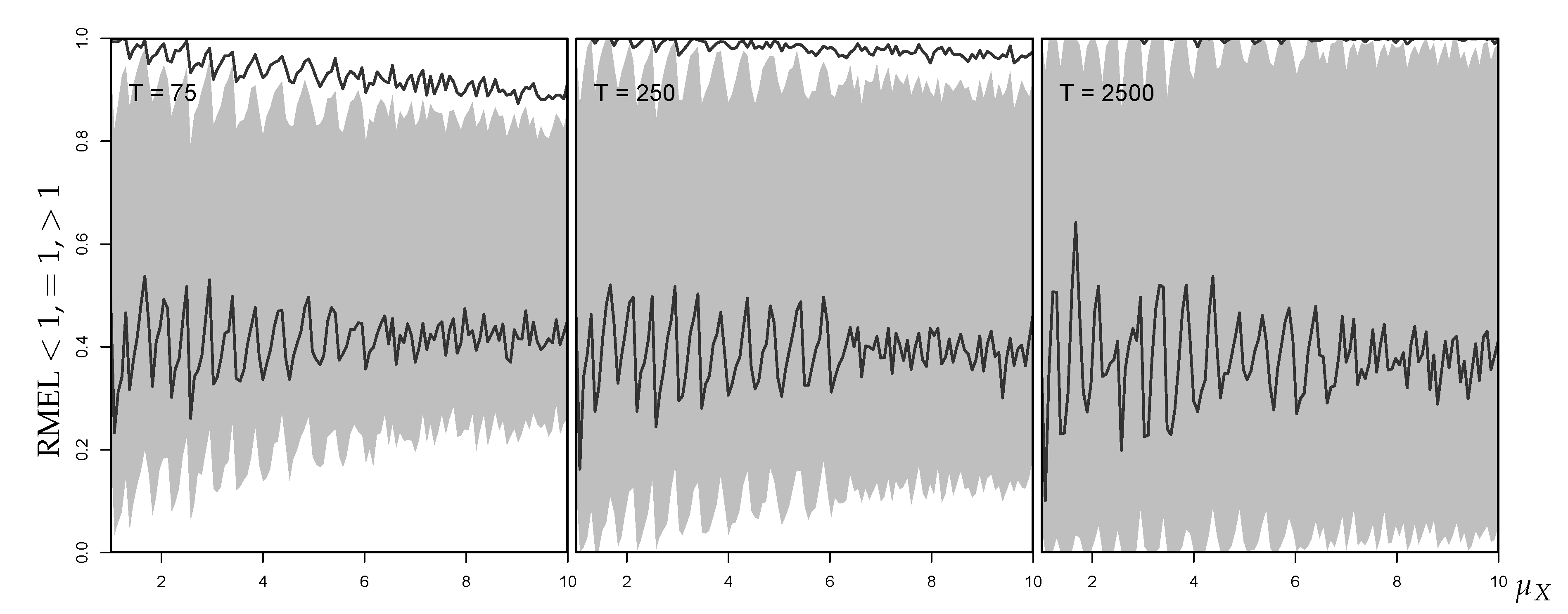
While the RMAE values show a quite stable behavior, the mean RMEL values for the 95%-quantile forecasts plotted on the right-hand side of Figure 10 show a lot of fluctuation (especially for small ). The Poi-INAR(1)’s mean RMEL values are typically larger than 1 (implying that the computed forecasts fall below the true ) and tend towards 1 with increasing . In contrast, the Gaussian AR(1)’s mean RMEL values are consistently smaller than 1 (computed forecast exceeds true ), and remaining so even with increasing .
The explanation for this is given in Figure 11. Here, the displayed areas express the percentages of the RMEL being , or (grey-white areas for Poi-INAR(1) forecasts, areas separated by black lines for Gaussian AR(1) ones). The percentages add up to 100% along the Y-axis: the distance between 0 and the lower bound of the grey area (lower black line) gives the percentage of simulation runs leading to RMEL , the height of the grey area (distance between black lines) the percentage of exact matches (RMEL ), and the upper distances the percentages for RMEL . According to Figure 11, the percentage of RMEL values generally decreases with growing (for both models) due to the increase in variance , but a growing T reduces this effect. For the Poi-INAR(1) model, growing T also considerably increases the percentage of RMEL values , with a balanced amount of RMEL and . For the Gaussian AR(1) model, in contrast, the percentage of RMEL values remains constant in T (roughly around 40%), and only the percentage of RMEL values decreases. This explains why the mean RMEL in Figure 10 tends towards a constant value below 1. Generally, for our Poi-INAR(1) simulations, we have at least 60% matches for the central forecast (RMAE ) if fitting a Poi-INAR(1) model, whereas the minimal hit rate is about 30% for the Gaussian approximation. For the forecast, we achieve at least 40% or 30% matches (RMEL ) if fitting a Poi-INAR(1) or Gaussian AR(1) model, respectively. Especially when fitting a Poi-INAR(1) model, these percentages increase noticeably with growing sample size T.
4. Point Forecasting for Diverse Types of DGPs
The baseline analysis regarding point forecasting for the Poi-INAR(1) DGP presented in Section 3 allowed us to introduce our forecasting approaches, to distinguish between approximation and estimation error, and to discuss possible variations of the experimental design. Now, we extend our analyses in a more streamlined way to several different types of DGP, as summarized in Figure 1 before. In Section 4.1, we continue with INAR(1) DGPs, but now having overdispersion or zero inflation. Then, we allow for higher-order autoregression in Section 4.2 by considering an INAR(2) process. In Section 4.3, we investigate the so-called INARCH family as an alternative AR type model for count processes. While all these DGPs have the full (unbounded) set as their range, Section 4.4 focuses on processes of bounded counts. Finally, Section 4.5 concludes by considering non-stationary count processes, which exhibit seasonality and trend in addition to an AR component.
4.1. Point Forecasts of INAR(1) Processes with Overdispersion or Zero Inflation
The most common violations of a Poisson assumption are overdispersion (i.e., a variance larger than the mean) and zero inflation (i.e., a larger zero probability than for a Poisson distribution having the same mean). Within the INAR(1) model, overdispersed observations can be generated by using a negative binomial distribution for the innovation’s, (see Weiß (2018)). For this NB-INAR(1) model, controls the innovations dispersion index: . Using Equation (A2) in Appendix A.2, we can find values for for any choice of the ’s mean and dispersion index, with . The true h-step-ahead forecast distribution is computed using Equations (A4) and (A5), and the approximation in Equation (7) results as
with . Analogously, the use of the zero-inflated Poisson distribution for the innovations (which adds an amount of zero probability while reducing the underlying -probabilities by ) causes zero-inflated INAR(1) observations (see Jazi et al. (2012)). Actually, the ZIP-innovations also cause overdispersion (with ). Similarly, NB-innovations also exhibit some degree of zero inflation. For the ZIP-INAR(1) model, we determine the true h-step-ahead INAR(1) forecast distribution again using Equations (A4) and (A5), and we approximate it by the Gaussian AR(1) model
with .
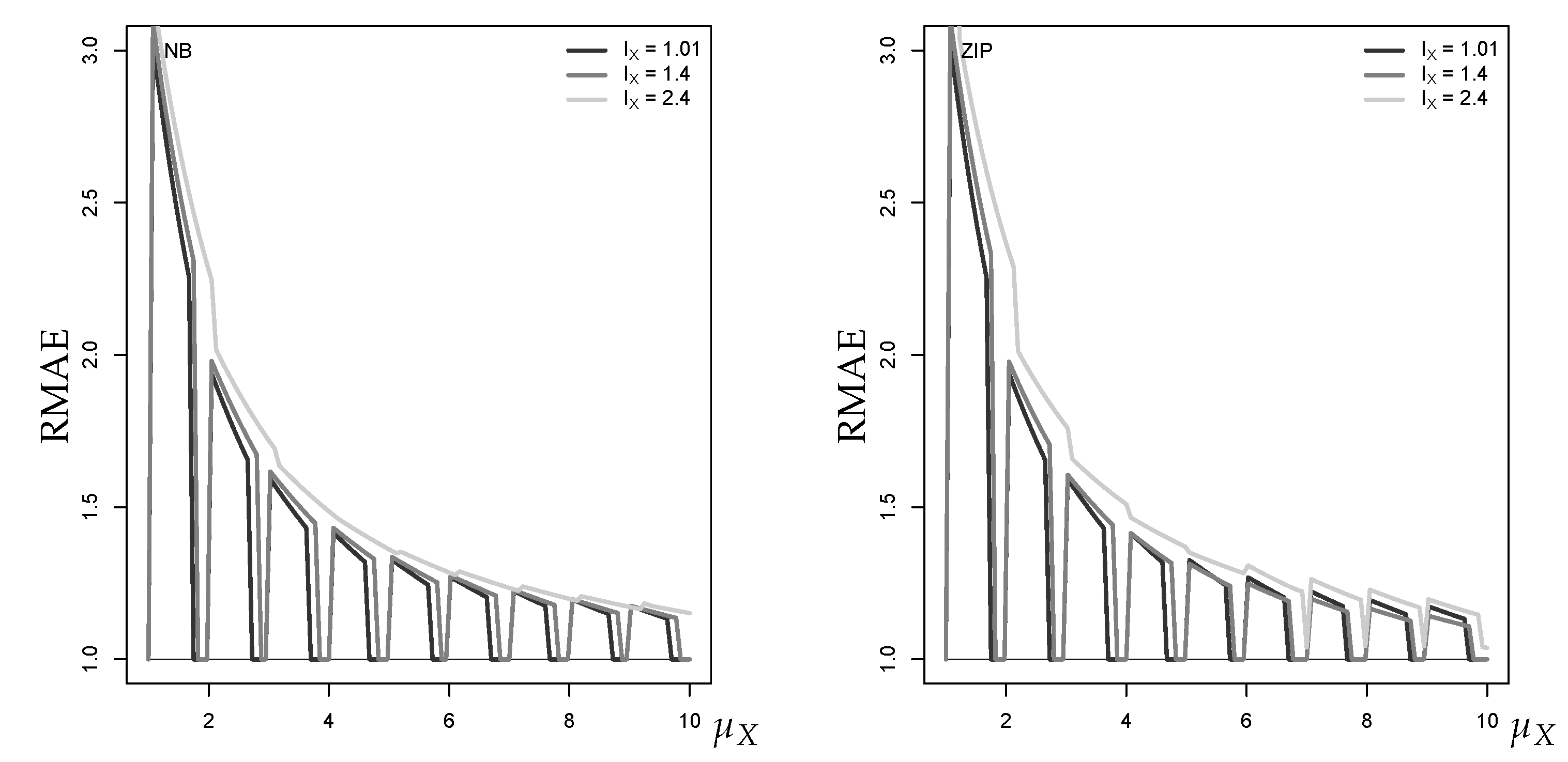
The effect of overdispersion and zero inflation on the RMAE of the approximate median forecast is generally rather small, deviations are only visible for a large autocorrelation level . Therefore, in Figure 12, we selected graphs with for illustration. There is not much difference between the case of an NB-INAR(1) process (left) or a ZIP-INAR(1) process (right). Except for a low mean such as , we do not see a strong effect of increased overdispersion or zero inflation on the goodness of approximation. The deterioration of approximation quality for small means can be explained as follows. Having fixed the marginal mean , the conditional means in Equations (9) and (10) and thus the approximate median forecasts are not further affected by overdispersion or zero inflation, and only the conditional variances are increased. The true median forecasts, however, tend more and more towards zero with increasing overdispersion and especially zero inflation, thus the forecast accuracy concerning the median deteriorates.
When evaluating the approximate of the 1-step-ahead forecast distribution with either NB- or ZIP-distributed innovations, the RMEL values are affected for all levels of . Figure 13 shows an illustrative example with . In both cases, the approximation error turns from RMEL (forecast exceeds true ) to RMEL (forecast falls below true ) with increasing , but mainly for large in the NB-case, and only for small in the ZIP-case. The tendency towards RMEL in the NB-case can be explained as follows: increasing overdispersion leads to more probability mass in the upper tail of the true forecast distribution and thus an increased , whereas the tails of the normal distribution are always light4. In the ZIP-case with large , in contrast, the additional dispersion is caused by the large distance between the zero and the remaining probability masses, so the upper tail does not much differ from the Poi-INAR(1) case.
Figure 14 plots the simulated mean RMEL values for under additional estimation uncertainty (with chosen as the respective last observation of the simulated time series). Both for the NB- and the ZIP-case, the mean RMEL of the INAR(1) forecasts tends towards a level near 1 with growing . The Gaussian approximations’ mean RMEL, in contrast, becomes increasingly larger than 1 (forecast below true ) in the NB-case, and smaller than 1 (forecast exceeds true ) in the ZIP case, confirming our discussion of Figure 13.
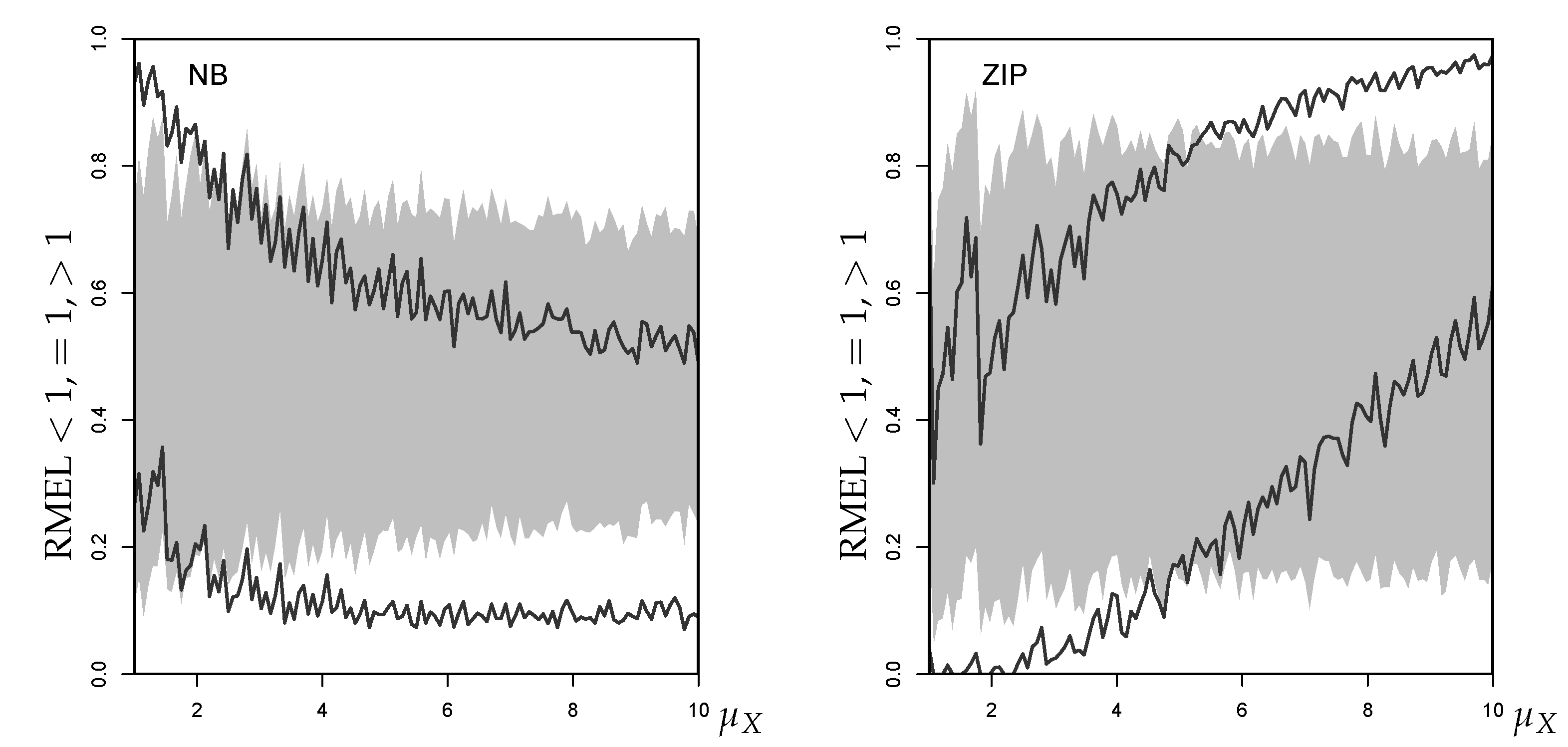
The reason for this change in the mean RMEL becomes obvious in Figure 15. Here, we see that for both DGPs, NB and ZIP, the percentages of RMEL values below and above 1 are fairly even if fitting an INAR(1) model to the data. With growing , the Gaussian AR(1) approximation of the NB model starts to produce a lot of RMEL values greater than 1, and the percentage for RMEL slightly decreases. In the ZIP-case, the approximation first produces mainly RMEL values , but changes to producing more RMEL values for . Thus, both cases lead to a biased RMEL performance, with a bias in opposite directions.
4.2. Point Forecasts of Poisson INAR(2) Processes
Until now, all considered models (and their approximations) have autoregressive order 1. Now, we extend to second-order autoregression and consider the Poisson INAR(2) model ; see Equations (A8) and (A9) in Appendix A.2 for further details. For given and , we computed and again generated 1000 replications per scenario. To approximate the Poi-INAR(2) process, we used its second-order counterpart, the Gaussian AR(2) process, and fit it to the simulated count time series. Based on the respective last two observations , point forecasts for both types of fitted model were computed.
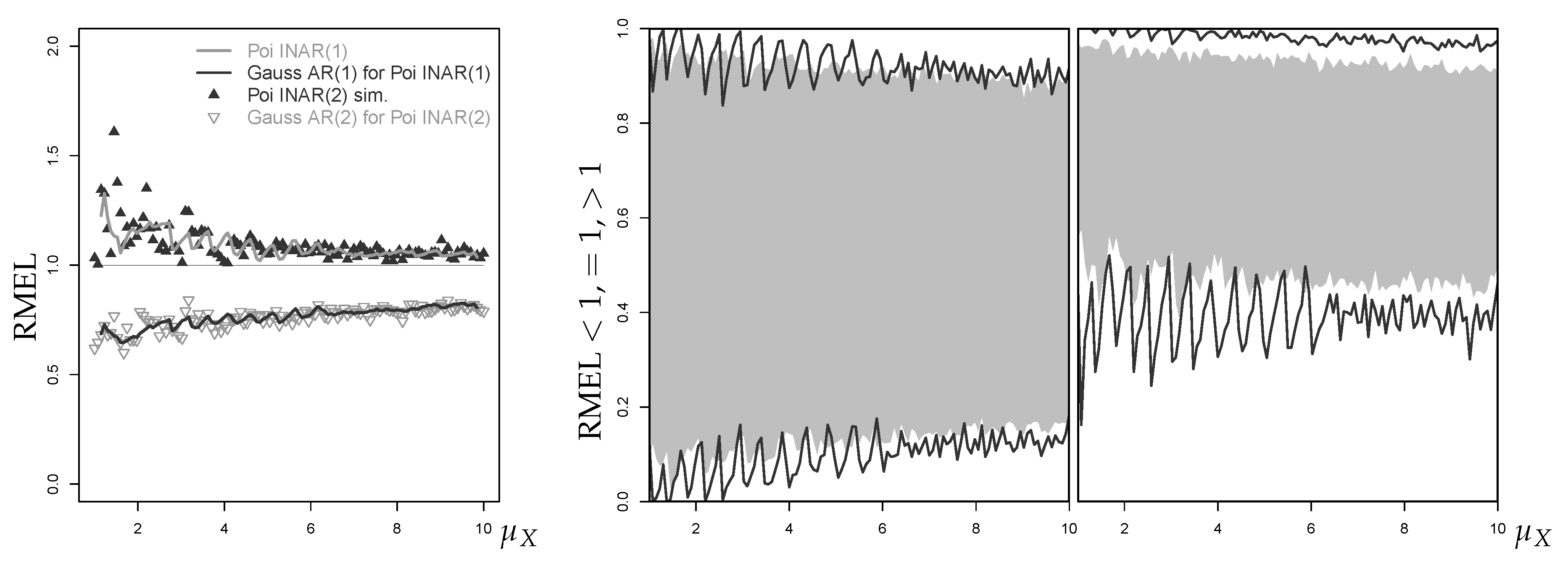
The respective first- and second-order Poi-INAR models produce rather similar results. For and , the RMAE values of the fitted Poi-INAR(2) model and its Gaussian approximation are very close to the values plotted in Figure 10 (also see the left part in Figure 18 below). For , the Gaussian approximation produces slightly reduced RMAE values compared to the first-order case. In addition, the conclusions regarding the approximation do not change for the second-order DGP as illustrated by Figure 16 for the simulation scenario , , . On the left-hand side, we see the mean RMEL of the fitted Poi-INAR(2) model and its Gaussian approximation as dots. To check for possible differences to the INAR(1) case in Figure 10 (right), but to keep Figure 16 readable at the same time, we applied a moving window of length 5 to the dots in Figure 10 and plotted the resulting smoothed mean RMEL values of the Poi-INAR(1) model and its approximation as solid lines. The other plots show the percentages of RMELs , , of the fitted Poi-INAR model (middle) and its approximation (right). We can see slightly lower percentages of exact point forecasts (RMEL ) than in the Poi-INAR(1) case, but the general behavior is the same for both model orders. Thus, while overdispersion or zero inflation may severely affect the approximate forecasting performance, the actual model order seems to be of minor importance in these regards.
4.3. Point Forecasts of INARCH Processes
Another type of AR-like models for counts are included in the INGARCH family; and these are often used as alternatives to the INAR model. In this section, we evaluate point forecasts of first- and second-order Poisson INARCH models (and their Gaussian AR approximations5) under estimation uncertainty; see Equations (A10) and (A11) in Appendix A.3 for background information.
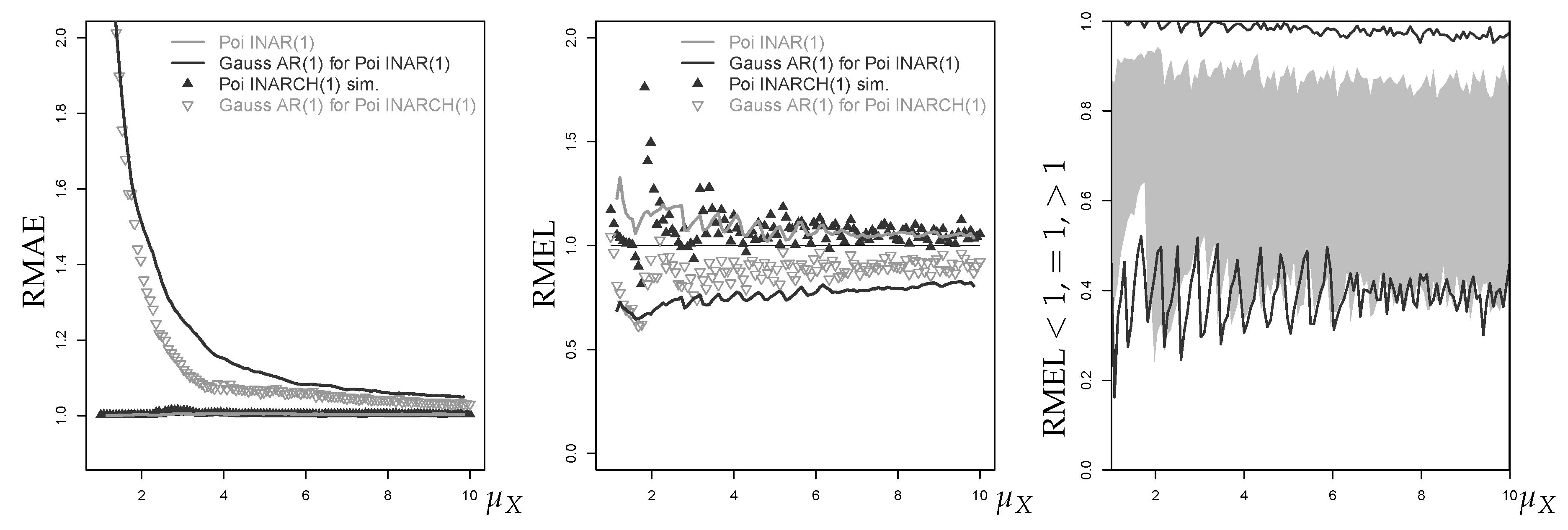
The performance of the median and forecast for the Poi-INARCH(1) model is generally quite similar to the Poi-INAR(1) case. However, for large autocorrelation parameter , the Gaussian approximation to the Poi-INARCH(1) model provides a better performance regarding central forecasts than in the Poi-INAR(1) case, in the sense of lower mean RMAE values for the approximate median forecast, see the left part of Figure 17. The middle graph shows that the mean RMEL values of the approximate forecast, though still constantly below 1, are closer to 1 than in the Poi-INAR(1) case. From the right part of Figure 17, however, we see that the percentage of correct forecasts (RMEL ) is even worse. The Gaussian AR(1) approximation of the Poi-INARCH(1) model just produces more RMEL values , which shifts the mean RMEL closer to 1.
The mean RMAE and RMEL values of the fitted Poi-INARCH(2) model and its approximation generally produce a very similar picture to that of the Poi-INARCH(1) model, but a growing slightly reduces the variation among the RMAE and RMEL values, see the right-most graph in Figure 18. A comparison between the different AR-like processes for counts is done in Figure 18. The mean RMAE values (left part) of the fitted Gaussian AR(2) approximation show the same overall behavior as in the Poi-INAR(2) case, and the same conclusion applies to the mean RMEL values in the right part of Figure 18. As the only difference, as in the first-order case in Figure 17, the Poi-INARCH(2) approximation’s mean RMEL values are somewhat closer to 1 than in the Poi-INAR(1) case. The reason is the same as before: the percentage of exact matches (RMEL ) is reduced at the cost of more cases with RMEL . However, besides these small differences, the specific type of AR-like DGP for counts does not have a notable effect on the forecasting performance, while other parameters such as the actual autocorrelation level are much more important.
4.4. Point Forecasts of Bounded Counts Processes
In the preceding sections, we examine forecasts of models with an infinite range of counts. Now, we turn to AR(1)-like count time series with a bounded range with some . This restriction is relevant if the counts are determined with respect to a population of specified (and typically low) size n (such as a fixed group of countries, companies or customers). Here, it may happen that (i.e., it is not possible to exceed the ), which, in turn, causes MEL values equal to 0 (see Equation (4)). However, in our simulations, this happened extremely rarely. The few cases where we had a division by zero when calculating the RMEL did not affect the computation of the truncated mean (as described in Section 3.5, the RMAE and RMEL values are averaged only after truncating their 10 smallest and largest values).
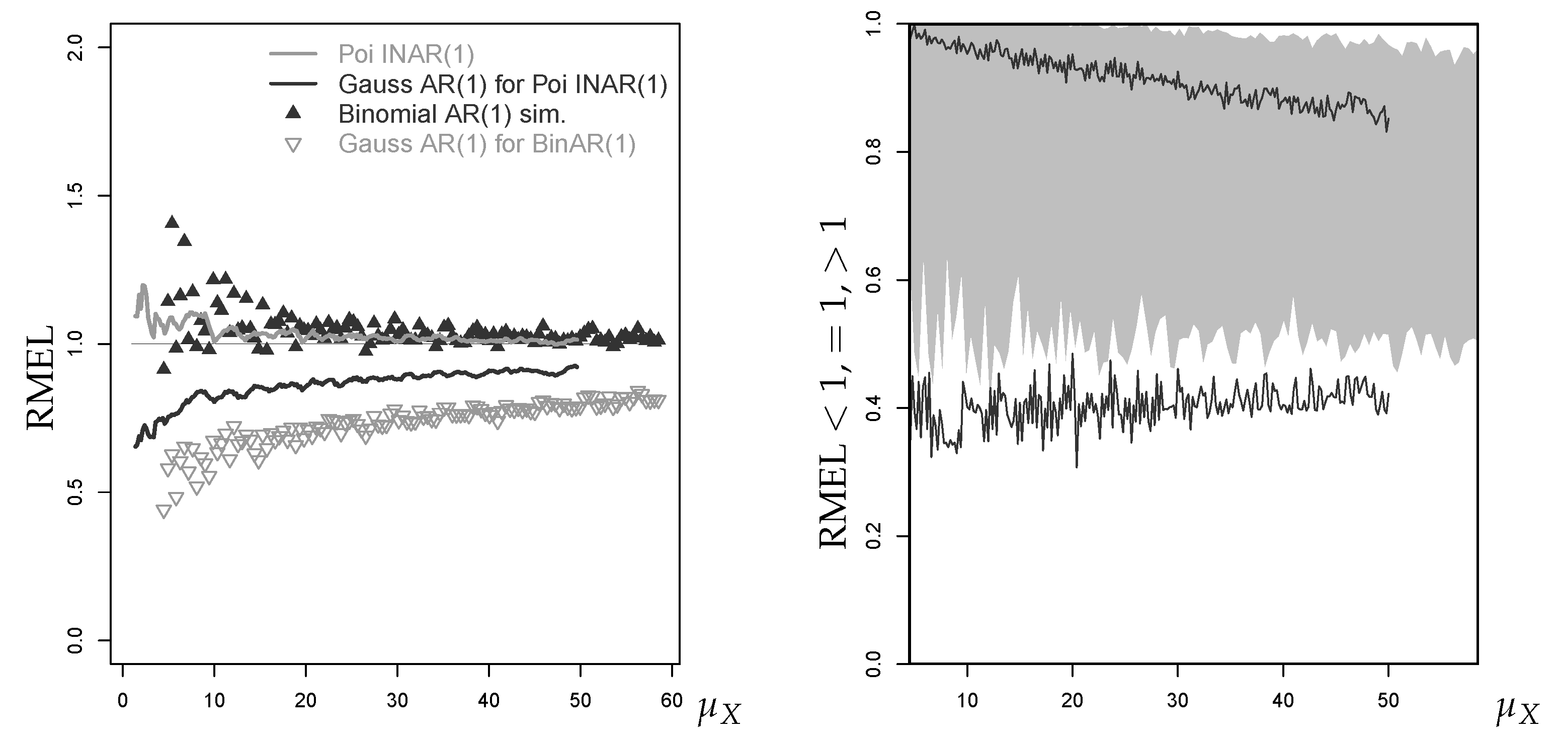
We start with the binomial AR(1) process having a binomial marginal distribution; see Equation (A6) and (A7) in Appendix A.2 for further details. However, we later also refer to binomial INARCH(1) processes, where the marginal distribution exhibits extra-binomial variation. The median forecast performance for BinAR(1) counts nearly coincides with the Poi-INAR(1) case from Section 3.5. While this also holds for the RMEL given a small (where binomial and Poisson distribution are quite similar to each other), the Gaussian approximation in the BinAR(1) case with performs quite differently from the one in the Poi-INAR(1) case. In the left plot of Figure 19, we see that the fitted Gaussian approximation in the BinAR(1) case provides much lower mean RMEL values than in the Poi-INAR(1) case. However, as shown in the right plot, the BinAR(1) approximation does not worse in terms of exact matches (RMEL ). It has a more biased RMEL performance, because it produces RMEL values very rarely. This leads to mean RMEL values being notably lower than in the Poi-INAR(1) case, and implies more frequent exceedances of the true . At this point, it is helpful to recall the discussions of Figure 2 and Figure 9. The Gaussian AR(1) approximation’s forecasts generally tend to exceed the true (RMEL ), also in the Poisson case. There, RMEL values can be assigned to the estimation error (more often in smaller samples), because it tends towards 0 for a growing sample size T. In the binomial case with , where the marginal distribution is close to symmetry, the estimation error does not seem to have such a strong effect.
We also considered the binomial INARCH(1) model as a DGP for bounded counts; see Equation (A12) and (A13) in Appendix A.3 for background information. The plots of the BinARCH(1) model look very similar to the BinAR(1) plots. In the case of deviation, they show the same behavior as the Poi-INARCH(1) model compared to the Poi-INAR(1) one (see Figure 17). For this reason, we do not further discuss them at this point.
4.5. Point Forecasts under Seasonality and Trend
As the final scenario, we allow the count DGP to be non-stationary by including both seasonality and trend. For this purpose, we use the ll-Poi-AR(1) model with period p given by Equation (A14) in Appendix A.3, which extends an AR(1)-like data-generating mechanism with a linear trend and harmonic oscillation for the log-means. Popular models for Gaussian time series with seasonality and trend are seasonal ARIMA (SARIMA) models and regression models with ARMA innovations (Brockwell and Davis 2016, Chapter 6), which both reduce to the ordinary ARMA models in the absence of seasonality and trend. Thus, we defined Gaussian approximations to the ll-Poi-AR(1) DGP by considering the SARIMA with period p on the one hand, and a regression model with AR(1) innovations on the other hand, having linear trend and harmonic oscillation as in Equation (A14). Since now the mean varies over time, we no longer evaluate our simulation results by plots against the mean, but we present tabulated values for illustration.
Let us start with some general findings. In our simulations, we considered different periods, but there was no effect on the predictive performance; therefore, we restrict the subsequent illustrations to (such as for monthly data). Furthermore, the Gaussian SARIMA approximation did considerably worse than the ARMA regression approximation in the majority of cases. This is plausible, because the true DGP has deterministic seasonality and trend as also assumed by the ARMA regression, whereas the SARIMA model assumes stochastic seasonality and trend. In view of this general result, we no longer consider the SARIMA approximation from this point on.
Table 1 shows mean RMAE and RMEL values and the corresponding percentages of RMAE or RMEL (in parentheses) for the sample sizes , with increasing trend parameter to the right, and increasing seasonality downwards. For the fitted ll-Poi-AR(1) model, the mean RMAEs are very close to 1, and the percentage of exactly matching the true conditional median is at least 70%. This percentage slightly deteriorates with increasing seasonality, but improves with sample size T. Although there is again more variation in the RMEL case, we essentially observe the same pattern also here. The Gaussian AR(1) regression approximation, in turn, leads to a much worse forecasting performance. Mean RMAEs are not smaller than 1.1, and the percentage of exact matches is only around 40% or worse. In addition, the exact matches of the true conditional (RMEL ) are clearly worse than in the ll-Poi-AR(1) case. In particular, these rates further decrease with both increasing trend or seasonality, and, often, they do not improve with increasing T.
We also varied the autoregressive parameter in as in the above sections, but a clear effect could not be recognized. In contrast, such an effect is visible if varying the intercept (controlling the baseline mean ). This is illustrated in Table 2 for (the case is provided by the lower part of Table 1). For the fitted ll-Poi-AR(1) model, the percentages of exact matches for both the central and non-central forecasts decrease with increasing . This result, which is in analogy to earlier results such as in Figure 11, can be explained with the conditional Poisson’s variance, which increases with increasing mean. However, although decreasing, these rates are much larger than those corresponding to the Gaussian approximation. Note that, for these larger values of , the Gaussian approximation also shows decreasing rates of RMEL for increasing trend or seasonality. Thus, we conclude that forecasts relying on a Gaussian approximation are even more problematic in the presence of seasonality and trend than in the stationary case.
5. Conclusions and Future Research
If coherent point forecasting is done based on a count time series model, then estimation error is nearly without effect on median forecasts. Non-central quantile forecasts, in contrast, are affected by estimation error, but the RMEL performance is more or less balanced and clearly improves with increasing sample size. If point forecasting relies on the discretization of a Gaussian ARMA approximation, the forecasting performance becomes considerably worse (both with and without estimation error). While the median forecast performance at least improves with increasing mean , non-central point forecasts show a strongly biased RMEL performance for any considered mean level. The RMEL performance is also severely affected by overdispersion or zero inflation, whereas neither the actual AR order nor the type of AR-like process (INAR vs. INARCH) leads to strong differences in forecasting performance. A bounded range may cause additional difficulties in approximating non-central point forecasts because of more frequent exceedances of the true quantile’s value. Finally, point forecasts for non-stationary processes of counts were also investigated and we found that the approximation of non-central point forecasts further deteriorates with increasing trend or seasonality.
To summarize, the practice of discretizing Gaussian ARIMA forecasts for count time series is strongly discouraged. For means , which are rather common values for real applications, non-central point forecasting should always rely on a count time series model. The same conclusion applies to central forecasts except the case of a low autocorrelation level, where the approximation leads to a reasonable performance also for somewhat smaller mean levels. It is telling that the Gaussian AR(1) forecast approximation is often outperformed by the basic EWMA approach, although the latter still does considerably worse than the model-based prediction.
There are a few directions for future research regarding the forecasting of count processes. One important direction is the construction and evaluation of (approximate) prediction intervals for count time series. Concerning (non-central) point forecasts, it would be interesting to incorporate costs into performance evaluation; especially the effect asymmetric cost schemes should be studied, where forecasts below or above the true quantile value go along with different costs. Finally, one may think of a risk-optimal parameter estimation for count time series, in the sense that estimates are determined by minimizing some measure of forecast errors for a given risk metric and risk level. In the context of risk optimization for discrete distributions, risk metrics different than VaR are often preferred, e.g., the expected shortfall, because the VaR has a multiextremum structure in this case (Larsen et al. 2002).
Author Contributions
Conceptualization (all authors); Funding acquisition (A.H., C.H.W.); Methodology (all authors); Software (A.H.); Supervision (C.H.W., L.C.A.); Writing—original draft preparation (A.H., C.H.W., L.C.A.); and Writing—review and editing (C.H.W., L.C.A., G.F. and R.G.).
Funding
This research was funded by the Deutsche Forschungsgemeinschaft (DFG, German Research Foundation)—Projektnummer 394832307.
Acknowledgments
The authors thank the two referees for their useful comments on an earlier draft of this article.
Conflicts of Interest
The authors declare no conflict of interest.
Appendix A. Considered Models for Count Time Series
This appendix provides a brief survey of those count time series models, which were used as a DGP in our numerical and simulation studies. More details and references on these and further count time series models can be found in the book by Weiß (2018).
Appendix A.1. Important Count Distributions
Let X be a count random variable. If the range of X is bounded from above by some upper limit , i.e., if X can only take values in , then the most common model is the binomial distribution with some . Its probability mass function (PMF) is given by
and mean and variance are equal to and , respectively.
If X can take values in the full set of non-negative integers, , then the Poisson distribution with constitutes an important model. Its PMF equals
Since mean and variance are equal to each other, both equal to , the Poisson distribution has the equidispersion property. A common model for unbounded counts with overdispersion is the negative binomial distribution with and , and with PMF
Its mean equals , whereas its variance is inflated by the factor , thus given by . If overdispersion is caused by zero inflation, one often uses the zero-inflated Poisson distribution with and ( corresponds to the -distribution). It has the PMF
and mean and variance are given by and , respectively.
Appendix A.2. Thinning-Based Models
is said to be an INAR process of order 1 (integer-valued autoregressive) if it follows the recursion
with independent and identically distributed (i.i.d.) innovations . The INAR(1) model uses the binomial thinning operator “∘” (Steutel and van Harn 1979). For and a count random variable N, binomial thinning is defined as , where is a sequence of i.i.d. Bernoulli random variables with , being independent of N. The thinning operations at each time t are performed independently of each other and of , and the are independent of (McKenzie 1985).
The autocorrelation function (ACF) is of AR(1)-type, given by . The mean and the dispersion index of the marginal distribution of the INAR(1) process are determined by
where I denotes the index of dispersion, and corresponds to the case of equidispersion (Weiß 2018). We speak of a Poisson INAR(1) process (Poi-INAR) following the recursion of Equation (A1) if the innovations are i.i.d. Poisson, . The marginal distribution is then also Poisson and thus equidispersed with . The h-step-ahead probability mass function (pmf) is given by
with conditional mean and variance (Freeland and McCabe 2004).
If the innovations’ distribution is not Poisson or not further specified, no closed-form formula is available for the h-step-ahead pmf with . The one-step-ahead pmf is given by
and the h-step-ahead forecast distribution is determined numerically by making use of the Markov property: for an M sufficiently large, we define the transition probability matrix
the entries of which are the desired h-step-ahead forecast probabilities (Weiß 2018).
The INAR(1) model in Equation (A1) cannot be used for time series of bounded counts, i.e., where the have the finite range with some . As a solution, McKenzie (1985) suggested replacing the innovation term by the additional thinning . More precisely, letting and , and defining and , the binomial AR(1) process follows the recursion
where again all thinnings are performed independently of each other, and independently of . The BinAR(1) model in Equation (A6) defines a stationary Markov chain with the binomial marginal distribution , and the ACF (which might also become negative). The one-step-ahead pmf equals
The h-step-ahead conditional distribution is computed according to Equation (A5) with .
In addition, higher-order extensions of Equation (A1) have been proposed in the literature. Here, we concentrate on the second-order case. The most widely used type of INAR(2) model is due to Du and Li (1991), who required conditional independence for the thinnings given in the extended model recursion
The one-step-ahead pmf equals
and h-step-ahead probabilities can be computed by adapting Equation (A5) to the bivariate Markov chain given by . The ACF satisfies and for .
Appendix A.3. Regression Models
Regression models for count time series assume a parametric relation for the counts’ conditional mean. Quite popular are so-called INGARCH models (integer-valued generalized autoregressive conditional heteroskedasticity), which assume a linear relation between the conditional mean and previous observations (Ferland et al. 2006). The actual count is then emitted by, e.g., a Poisson distribution having mean (Poi-INGARCH), but other types of count distribution could be used as well (Weiß 2018). The Poi-INARCH(2) model assumes
with , and it reduces to the Poi-INARCH(1) model if and . The ACF is computed in the same way as for the respective INAR model. The one-step-ahead pmf equals
this reduces to by setting . The h-step-ahead probabilities can be computed by adapting Equation (A5). An INARCH(1) model for bounded counts was proposed by Weiß and Pollett (2014); their binomial INARCH(1) model is defined by
with . Setting and , a BinARCH(1) process has the same mean and ACF as the corresponding BinAR(1) process, but a larger variance (extra-binomial variation). The one-step-ahead pmf equals
and the h-step-ahead conditional distribution is computed according to Equation (A5) with .
Zeger and Qaqish (1988) proposed an AR-like Poisson regression model for unbounded counts with an additional log-link, which allows to incorporate covariate information like deterministic trend and seasonality. In Section 4.5, we consider this log-linear Poisson AR(1) model (ll-Poi-AR(1) model) together with a linear trend and a harmonic oscillation with period p (and hence angular frequency ), given by
For , we have a purely autoregressive model. In our simulations, we actually used a harmonic oscillation based on with randomly drawn from such that predictions may happen at each position within a cycle. Omitting the covariate part in Equation (A14), one ends up with an AR(1)-like model for counts, where the ACF may also take negative values depending on the sign of .
Appendix A.4. Computation of Inaccuracy Measures
The inaccuracy measures defined in Section 2 are computed based on the true DGP’s forecast distribution, for (see Appendix A.2 and Appendix A.3 for the respective formulae). The MAE in Equation (2) with respect to the forecast value is computed as the finite sum
where the upper limit M is either set equal to n in the case of a bounded range (then the computed sum even leads to the exact value of MAE), or it is chosen “sufficiently large” for an unbounded range. In our case, we determined M such that . Analogously, the MEL in Equation (4) is computed as
Appendix B. About Gaussian Approximations of INAR(1) Processes
Let be an INAR(1) process as described in Appendix A.2, and the be the corresponding approximating Gaussian AR(1) process in Equation (6). The variance of Equation (6) differs from the variance of the INAR(1) process in Equation (A2):
It is not possible to match both the observations’ and the innovations’ variance simultaneously. Therefore, Homburg (2018) distinguished between two approaches: the ϵ-method is motivated by conformably modeling the innovations, thus the Gaussian approximation is defined by
To obtain agreement within the observations, in contrast, the Gaussian innovations can be defined according to the X-method:
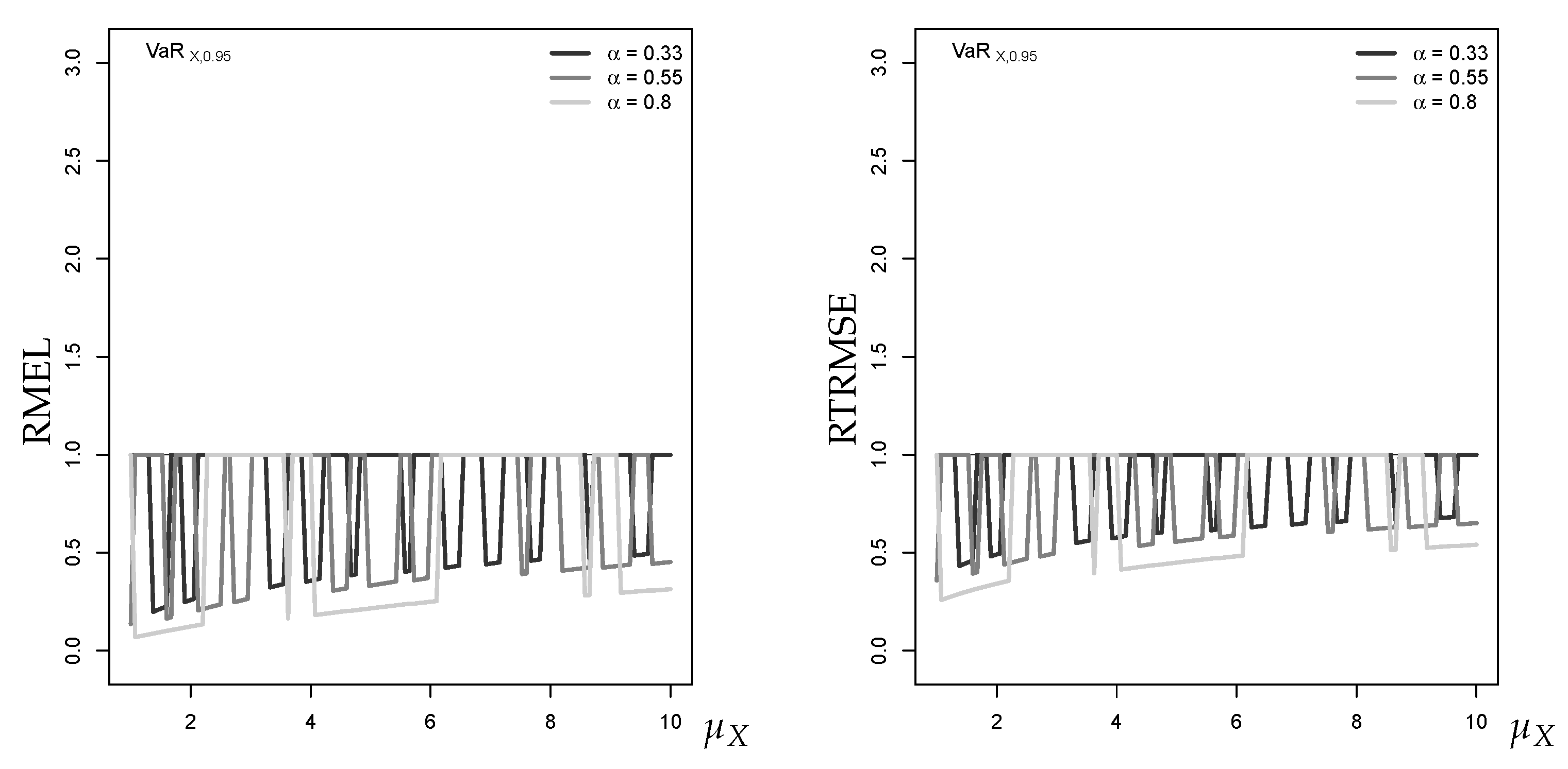
If computing the median as a central forecast, only the conditional mean of the Gaussian AR(1) approximation in Equation (7) is relevant, which does not depend on . Choosing , there is no difference between the X- and -method for this type of central forecast. For the mode, there might be an effect in special cases, also see the discussion in Appendix D, but usually, also this type of central point forecast is not affected by the X- or -method. If approximating quantiles in the upper tail region (non-central forecasts), however, the X-method outperforms the -method. This is illustrated by Figure A1, according to which the -method often causes RMEL (forecast below ), while the X-method has RMEL and is hence more conservative. As a consequence, we decided to use the X-method in this work.
Figure A1.
RMEL for 95%-quantile forecast approximation against ((left) X-method; and (right) -method), with horizon , where equals median of marginal distribution.
Figure A1.
RMEL for 95%-quantile forecast approximation against ((left) X-method; and (right) -method), with horizon , where equals median of marginal distribution.

Appendix C. MSE-Based Performance Evaluation of Point Forecasts
In this work, we use the MAE to evaluate the median forecast as a central forecast, and the MEL defined by Equation (4) for the non-central quantile forecasts. Other widely used performance measures are defined based on mean squared errors, namely
for evaluating central forecasts, and the corresponding tail version
for non-central forecasts. The RMSE is minimized by the conditional mean, which, for a Gaussian approximation, coincides with the conditional median as well as the mode. For the right-skewed conditional distribution of the Poi-INAR(1) process, we often observe . Thus, the RMSE is usually not minimized by the median forecast considered in this work, and it will lead to different values than the MAE. To compare the performance measures RMAE and RMEL with the MSE-based ones, we also computed the relative measures
Figure A2 shows the RMAE and RRMSE of the (approximate) median forecasts for a Poi-INAR(1) process. We see that the main conclusions from both graphs coincide: the relative error tends towards 1 with increasing , and is larger for larger levels of the autocorrelation parameter . Thus, RRMSE does not provide further insights into the approximation quality.
As illustrated by Figure A3, also the RMEL and RTRMSE both provide essentially the same message about the approximations’ forecast performance, namely that the forecasts tend to exceed (RMEL and RTRMSE ). Furthermore, both graphs show that with increasing , the approximation quality improves. Thus, again, there is no benefit if considering RTRMSE as a further metric for approximation quality.
Figure A2.
RMAE (left) and RRMSE (right) for median forecast approximation against , with horizon , where equals median of marginal distribution.
Figure A2.
RMAE (left) and RRMSE (right) for median forecast approximation against , with horizon , where equals median of marginal distribution.

Figure A3.
RMEL (left) and RTRMSE (right) for 95%-quantile forecast approximation against , with horizon , where equals median of marginal distribution.
Figure A3.
RMEL (left) and RTRMSE (right) for 95%-quantile forecast approximation against , with horizon , where equals median of marginal distribution.

Appendix D. About the Mode as a Coherent Central Point Forecast
Another possibility for a coherent central point forecast is the mode. While median and mode always coincide for a symmetric unimodal distribution, they might differ for the skewed conditional distributions of count models. The decision between median and mode as a central point forecast has to be done based on practical reasoning: the mode is motivated as being the most probable outcome, whereas the median expresses the center of the distribution in a probabilistic sense. A reason against the use of the mode is the possibility of multiple modes. The mode might also be misleading in the presence of zero inflation, and it does not have a “non-central counterpart.” Furthermore, while the approximate median just corresponds to the ceiled Gaussian median, the discretization may cause the approximate mode to deviate from the ceiled Gaussian mode (=median). As an example, if we have a strong degree of overdispersion (i.e., if is much larger than ), it may happen that the approximate discrete zero probability, i.e., , is maximal within the pmf although the median is larger than 0. For an NB-INAR(1) process with , and with being the median of the marginal distribution, the true one-step-ahead forecast pmf has median 3 and mode 2. The Gaussian approximation in Equation (9) has conditional mean , thus ceiling leads to the approximate median forecast 5. However, because of the large conditional variance (≈17.8), the approximate zero probability becomes largest within the approximate forecast pmf, i.e., the approximate mode equals 0. Thus, approximate mode and median deviate heavily from each other.
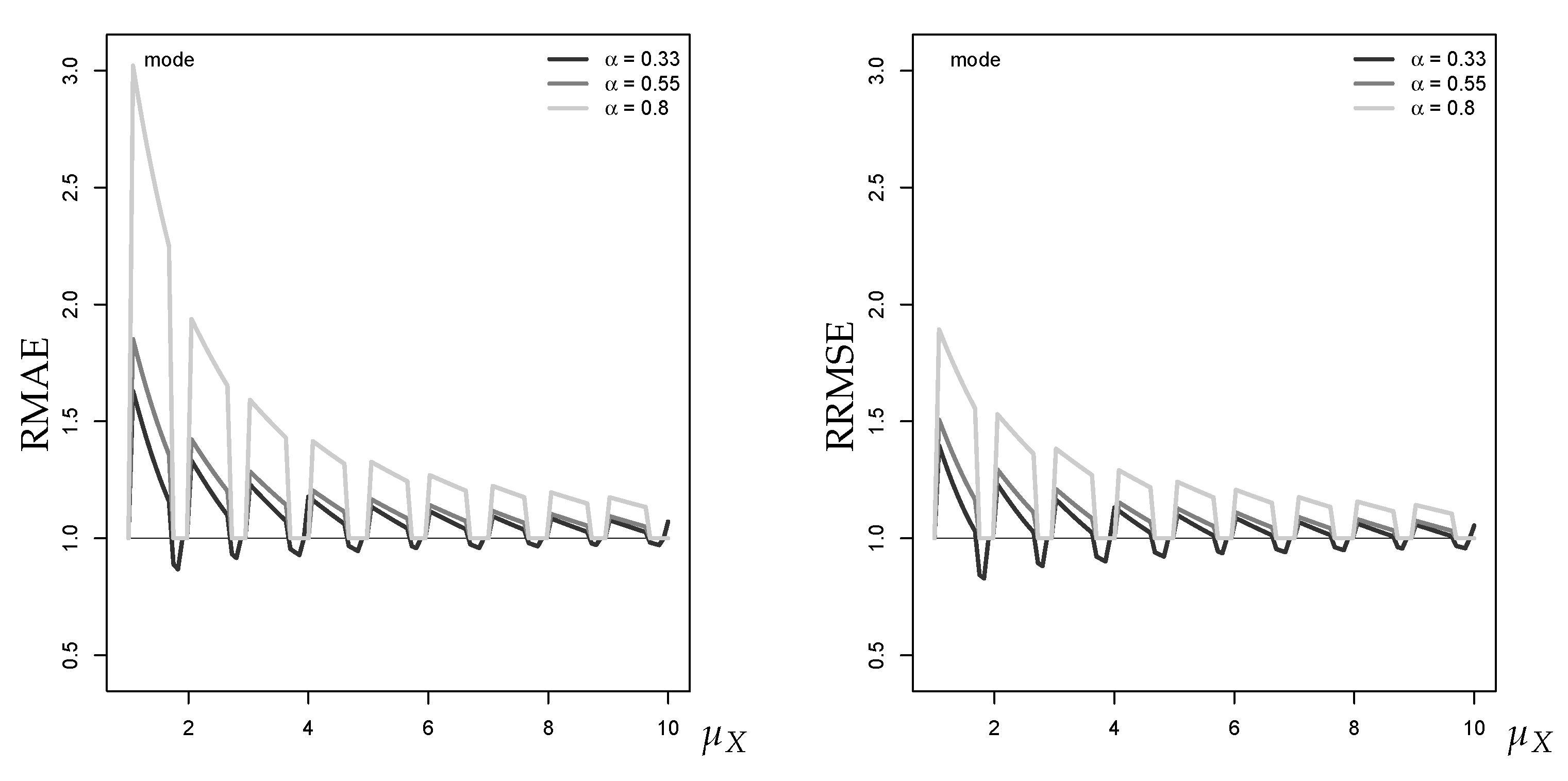
Furthermore, the popular forecast error measures RMAE and RRMSE (see Appendix C) might both be misleading if being applied to mode forecasts. If looking at Figure A4 regarding the Gaussian approximation of a Poi-INAR(1) DGP, both RMAE and RRMSE sometimes fall below 1, which would indicate that the approximate mode forecast is more accurate than the true mode. However, the RMAE of the mode forecast falls below 1 if the approximated mode is closer to the median of the Poi-INAR(1) forecast distribution than the true mode, since the MAE is minimized by the median (analogously, the RMSE is minimized by the mean). This gets even clearer with the following numerical example: assume , then for , the true one-step-ahead mode equals 2 and the median 3. For the Gaussian approximation, the conditional mean is 2.799, and the approximate mode and median forecast are 3. Thus, while both median forecasts are equal (hence ), the mode forecasts differ (approximation error). Both relative measure lead to a value smaller than 1 if applied to the modes: and . This can be explained by the fact that the approximate mode forecast 3 is closer to the conditional median 3 or to the conditional mean 2.799, respectively, than the true mode 2.
Figure A4.
RMAE (left) and RRMSE (right) for mode forecast approximation against , with horizon , where equals median of marginal distribution.
Figure A4.
RMAE (left) and RRMSE (right) for mode forecast approximation against , with horizon , where equals median of marginal distribution.

References
- Alwan, Layth C., and Christian H. Weiß. 2017. INAR implementation of newsvendor model for serially dependent demand counts. International Journal of Production Research 55: 1085–99. [Google Scholar] [CrossRef]
- Bisaglia, Luisa, and Antonio Canale. 2016. Bayesian nonparametric forecasting for INAR models. Computational Statistics and Data Analysis 100: 70–78. [Google Scholar] [CrossRef]
- Bisaglia, Luisa, and Margherita Gerolimetto. 2015. Forecasting integer autoregressive processes of order 1: Are simple AR competitive? Economics Bulletin 35: 1652–60. [Google Scholar]
- Box, George EP, and Gwilym M. Jenkins. 1970. Time Series Analysis: Forecasting and Control, 1st ed. San Francisco: Holden-Day. [Google Scholar]
- Brockwell, Peter J., and Richard A. Davis. 2016. Introduction to Time Series and Forecasting, 3rd ed. Basel: Springer International Publishing Switzerland. [Google Scholar]
- Christoffersen, Peter F., and Francis X. Diebold. 1997. Optimal prediction under asymmetric loss. Econometric Theory 13: 808–17. [Google Scholar] [CrossRef]
- Du, Jin-Guan, and Yuan Li. 1991. The integer-valued autoregressive (INAR(p)) model. Journal of Time Series Analysis 12: 129–42. [Google Scholar]
- Ferland, René, Alain Latour, and Driss Oraichi. 2006. Integer-valued GARCH processes. Journal of Time Series Analysis 27: 923–42. [Google Scholar] [CrossRef]
- Freeland, R. Keith, and Brendan PM McCabe. 2004. Forecasting discrete valued low count time series. International Journal of Forecasting 20: 427–34. [Google Scholar] [CrossRef]
- Gneiting, Tilmann. 2011. Quantiles as optimal point forecasts. International Journal of Forecasting 27: 197–207. [Google Scholar] [CrossRef]
- Göb, Rainer. 2011. Estimating Value at Risk and conditional Value at Risk for count variables. Quality and Reliability Engineering International 27: 659–72. [Google Scholar] [CrossRef]
- Hendricks, Darryll. 1996. Evaluation of value-at-risk models using historical data. Economic Policy Review 2: 39–69. [Google Scholar] [CrossRef]
- Homburg, Annika. 2018. Criteria for evaluating approximations of count distributions. Communications in Statistics—Simulation and Computation. forthcoming. [Google Scholar] [CrossRef]
- Jazi, Mansour A., Geoff Jones, and Chin-Diew Lai. 2012. First-order integer valued AR processes with zero inflated Poisson innovations. Journal of Time Series Analysis 33: 954–63. [Google Scholar] [CrossRef]
- Jolliffe, Ian T. 1995. Sample sizes and the central limit theorem: The Poisson distribution as an illustration. American Statistician 49: 269. [Google Scholar]
- Jung, Robert C., and Andrew R. Tremayne. 2006. Coherent forecasting in integer time series models. International Journal of Forecasting 22: 223–38. [Google Scholar] [CrossRef]
- Larsen, Nicklas, Helmut Mausser, and Stanislav Uryasev. 2002. Algorithms for optimization of value-at-risk. In Financial Engineering, E-commerce and Supply Chain. Edited by Panos M. Pardalos and Vassilis Tsitsiringos. Boston: Springer. [Google Scholar]
- Lopez, Jose A. 1998. Methods for evaluating Value-at-Risk estimates. Economic Policy Review 4: 119–24. [Google Scholar] [CrossRef]
- Maiti, Raju, Atanu Biswas, and Samarjit Das. 2016. Coherent forecasting for count time series using Box-Jenkins’s AR(p) model. Statistica Neerlandica 70: 123–45. [Google Scholar] [CrossRef]
- McCabe, Brendan PM, and Gael M. Martin. 2005. Bayesian predictions of low count time series. International Journal of Forecasting 21: 315–30. [Google Scholar] [CrossRef]
- McCabe, Brendan PM, Gael M. Martin, and David Harris. 2011. Efficient probabilistic forecasts for counts. Journal of the Royal Statistical Society, Series B 73: 253–72. [Google Scholar] [CrossRef]
- McKenzie, Ed. 1985. Some simple models for discrete variate time series. Water Resources Bulletin 21: 645–50. [Google Scholar] [CrossRef]
- Quddus, Mohammed A. 2008. Time series count data models: An empirical application to traffic accidents. Accident Analysis and Prevention 40: 1732–41. [Google Scholar] [CrossRef]
- Shcherbakov, Maxim V., Adriaan Brebels, Nataliya L. Shcherbakova, Anton P. Tyukov, Timur A. Janovsky, and Valeriy A. Kamaev. 2013. A survey of forecast error measures. World Applied Sciences Journal 7: 119–34. [Google Scholar]
- Silva, Nélia, Isabel Pereira, and M. Eduarda Silva. 2009. Forecasting in INAR(1) model. REVSTAT 24: 171–6. [Google Scholar]
- Steutel, Fred W., and Klaas van Harn. 1979. Discrete analogues of self-decomposability and stability. Annals of Probability 7: 893–9. [Google Scholar] [CrossRef]
- Su, Chun, and Qi-he Tang. 2003. Characterizations on heavy-tailed distributions by means of hazard rate. Acta Mathematicae Applicatae Sinica, English Series 19: 135–42. [Google Scholar] [CrossRef]
- Weiß, Christian H. 2018. An Introduction to Discrete-Valued Time Series. Chichester: John Wiley and Sons, Inc. [Google Scholar]
- Weiß, Christian H., and Philip K. Pollett. 2014. Binomial autoregressive processes with density dependent thinning. Journal of Time Series Analysis 35: 115–32. [Google Scholar] [CrossRef]
- Zeger, Scott L., and Bahjat Qaqish. 1988. Markov regression models for time series: A quasi-likelihood approach. Biometrics 44: 1019–31. [Google Scholar] [CrossRef] [PubMed]
| 1 | In a risk context (see Göb 2011), the term “conditional VaR” is sometimes used synonymously with the tail conditional expectation or to the expected shortfall. These measures provide additional information about the mean extend of an exceedance of Va and do thus not lead to integer values. |
| 2 | Alternative ways of discretizing a real-valued forecast would be rounding (to the nearest integer; this corresponds to the Gaussian approximation with continuity correction) or flooring (i.e., mapping real numbers x to the greatest integer ), but these are not further considered here. Note that, in the work by Homburg (2018), the median approximation with ceiling or with rounding lead to similar results, whereas the Va approximation was improved by using ceiling (or no continuity correction, respectively). |
| 3 | Usually, this restriction is not problematic because positive autocorrelation is most commonly encountered in practice. However, there are also models for count time series allowing for negative autocorrelation (see Appendix A for details). |
| 4 | The tail behavior of the normal and the NB distribution can be distinguished, for example, based on the mean excess for a given threshold value (see Su and Tang 2003). While converges to 0 with increasing c in case of a normal distribution, it can converge to any positive real number for an NB-distribution. |
| 5 | We still use a Gaussian AR approximation, not ARCH approximation. Despite their controversial name (Weiß 2018), the INARCH models are just AR-type models for count processes (see Appendix A.3). |
Figure 1.
Overview of considered DGPs.

Figure 2.
RMAE for median forecast approximation against (left), and RMEL for 95%-quantile forecast approximation (right), with horizon , where equals median of marginal distribution.
Figure 2.
RMAE for median forecast approximation against (left), and RMEL for 95%-quantile forecast approximation (right), with horizon , where equals median of marginal distribution.

Figure 3.
RMEL for (left) 99%- and (right) 99.5%-quantile forecast approximation against , with horizon , where equals median of marginal distribution.
Figure 3.
RMEL for (left) 99%- and (right) 99.5%-quantile forecast approximation against , with horizon , where equals median of marginal distribution.

Figure 4.
RMAE for median forecast approximation against , with horizon and different , where equals either 50%-, 50%-, or 75%-quantile of marginal distribution.
Figure 4.
RMAE for median forecast approximation against , with horizon and different , where equals either 50%-, 50%-, or 75%-quantile of marginal distribution.

Figure 5.
RMEL for 95%-quantile forecast approximation against , with horizon and different , where equals either 50%-, 50%-, or 75%-quantile of marginal distribution.
Figure 5.
RMEL for 95%-quantile forecast approximation against , with horizon and different , where equals either 50%-, 50%-, or 75%-quantile of marginal distribution.

Figure 6.
RMAE for median forecast approximation against , with different and varying horizons h, where equals median of marginal distribution.
Figure 6.
RMAE for median forecast approximation against , with different and varying horizons h, where equals median of marginal distribution.

Figure 7.
RMEL for 95%-quantile forecast approximation against , with different and varying horizons h, where equals median of marginal distribution.
Figure 7.
RMEL for 95%-quantile forecast approximation against , with different and varying horizons h, where equals median of marginal distribution.

Figure 8.
Mean of simulated RMAE values for median forecast against , with horizon , , and different sample sizes T, where equals median of marginal distribution.
Figure 8.
Mean of simulated RMAE values for median forecast against , with horizon , , and different sample sizes T, where equals median of marginal distribution.

Figure 9.
Mean of simulated RMEL values for 95%-quantile forecast against , with horizon , , and different sample sizes T, where equals median of marginal distribution.
Figure 9.
Mean of simulated RMEL values for 95%-quantile forecast against , with horizon , , and different sample sizes T, where equals median of marginal distribution.

Figure 10.
Mean of simulated RMAE values for median forecast (left) and RMEL values for 95%-quantile forecast (right) against , with horizon , , and size , where equals respective last observation of simulated time series.
Figure 10.
Mean of simulated RMAE values for median forecast (left) and RMEL values for 95%-quantile forecast (right) against , with horizon , , and size , where equals respective last observation of simulated time series.

Figure 11.
Percentages of RMEL values for 95%-quantile forecast being (central area), (lower area), and (upper area) against , with horizon , , and different sample sizes T, where equals respective last observation of simulated time series. Grey area corresponds to Poi-INAR(1) forecasts, areas separated by black line to Gaussian AR(1) forecasts.

Figure 12.
RMAE for median forecast approximation of NB-INAR(1) (left) and ZIP-INAR(1) process (right) against , with horizon , , and different , where equals to median of marginal distribution.
Figure 12.
RMAE for median forecast approximation of NB-INAR(1) (left) and ZIP-INAR(1) process (right) against , with horizon , , and different , where equals to median of marginal distribution.

Figure 13.
RMEL for 95%-quantile forecast approximation of NB-INAR(1) (left) and ZIP-INAR(1) process (right) against , with horizon , , and different , where equals to median of marginal distribution.
Figure 13.
RMEL for 95%-quantile forecast approximation of NB-INAR(1) (left) and ZIP-INAR(1) process (right) against , with horizon , , and different , where equals to median of marginal distribution.

Figure 14.
Mean of simulated RMEL values for 95%-quantile forecast of NB-INAR(1) (left) and ZIP-INAR(1) process (right) against , with horizon , , size , and , where equals respective last observation of simulated time series.
Figure 14.
Mean of simulated RMEL values for 95%-quantile forecast of NB-INAR(1) (left) and ZIP-INAR(1) process (right) against , with horizon , , size , and , where equals respective last observation of simulated time series.

Figure 15.
Percentages of RMEL values , , for 95%-quantile forecast of NB-INAR(1) (left) and ZIP-INAR(1) process (right) against , with horizon , , size , and , where equals respective last observation of simulated time series. Grey area corresponds to INAR(1) forecasts, areas separated by black line to Gaussian AR(1) forecasts.

Figure 16.
RMEL for 95%-quantile forecast of Poi-INAR(2) process, with horizon , , , and size , where equal last observations of simulated time series. (Left) Mean of simulated RMEL values against ; solid lines correspond to smoothed values of Poi-INAR(1) case. (Right) Percentage of RMEL , , for Poi-INAR(2) forecast (first graph) and for Gaussian AR(2) forecast (second graph) as grey areas; solid lines correspond to respective Poi-INAR(1) values.

Figure 17.
Poi-INARCH(1) DGP with horizon and size , where equals respective last observation of simulated time series; all plots against . (Left) Mean of RMAE values for median forecast, where ; solid lines correspond to smoothed values of Poi-INAR(1) case. (Center) Mean of RMEL values for 95%-quantile forecast, where ; solid lines correspond to smoothed values of Poi-INAR(1) case. (Right) Percentages of RMEL , , for Gaussian approximations to Poi-INARCH(1) (areas) or Poi-INAR(1) DGP (lines), where .

Figure 18.
RMAE for median forecast (left) and RMEL for 95%-quantile forecast (right) against : DGP Poi-INAR(2) vs. Poi-INARCH(2), with horizon , , , and size , where equal last observations of simulated time series; solid lines correspond to smoothed values of Poi-INAR(1) or Poi-INARCH(1) case, respectively.

Figure 19.
95%-quantile forecast against , with horizon , , and size , where equals last observation of simulated time series. (Left) Mean of simulated RMEL values for BinAR(1) DGP (dots); solid lines correspond to smoothed values of Poi-INAR(1) case. (Right) Percentages of RMEL , , for Gaussian approximations to BinAR(1) (areas) vs. Poi-INAR(1) DGP (lines).


Table 1.
Mean RMAE and RMEL values (percentages of RMAE or RMEL in parentheses) for ll-Poi-AR(1) DGP with , , and . Forecasts for fitted ll-Poi-AR(1) or Gaussian AR(1) regression model (labeled as “Poi” or “Gau,” respectively), sample size vs. .
Table 1.
Mean RMAE and RMEL values (percentages of RMAE or RMEL in parentheses) for ll-Poi-AR(1) DGP with , , and . Forecasts for fitted ll-Poi-AR(1) or Gaussian AR(1) regression model (labeled as “Poi” or “Gau,” respectively), sample size vs. .
| RMAE | RMEL | ||||||||||||
|---|---|---|---|---|---|---|---|---|---|---|---|---|---|
| 0 | 0.001 | 0.002 | 0 | 0.001 | 0.002 | ||||||||
| Poi | Gau | Poi | Gau | Poi | Gau | Poi | Gau | Poi | Gau | Poi | Gau | ||
| 0 | 0 | 1.011 | 1.186 | 1.012 | 1.185 | 1.012 | 1.178 | 1.604 | 1.078 | 1.401 | 1.044 | 1.093 | 0.889 |
| (0.874) | (0.386) | (0.880) | (0.350) | (0.849) | (0.280) | (0.691) | (0.679) | (0.699) | (0.607) | (0.741) | (0.589) | ||
| 0.1 | 0.3 | 1.026 | 1.186 | 1.027 | 1.188 | 1.029 | 1.175 | 1.359 | 0.939 | 1.339 | 1.043 | 1.304 | 1.109 |
| (0.769) | (0.395) | (0.763) | (0.361) | (0.750) | (0.398) | (0.611) | (0.486) | (0.603) | (0.509) | (0.579) | (0.501) | ||
| 0.2 | 0.6 | 1.028 | 1.183 | 1.029 | 1.198 | 1.026 | 1.186 | 1.450 | 0.996 | 1.326 | 1.042 | 1.356 | 1.225 |
| (0.743) | (0.387) | (0.759) | (0.365) | (0.721) | (0.376) | (0.633) | (0.424) | (0.603) | (0.367) | (0.599) | (0.370) | ||
| 0 | 0 | 1.002 | 1.195 | 1.003 | 1.131 | 1.006 | 1.102 | 1.348 | 0.949 | 1.174 | 1.100 | 0.897 | 1.105 |
| (0.944) | (0.365) | (0.835) | (0.273) | (0.900) | (0.388) | (0.849) | (0.766) | (0.851) | (0.638) | (0.755) | (0.536) | ||
| 0.1 | 0.3 | 1.007 | 1.154 | 1.007 | 1.149 | 1.009 | 1.108 | 1.203 | 0.845 | 1.219 | 1.033 | 1.169 | 1.266 |
| (0.862) | (0.408) | (0.856) | (0.345) | (0.814) | (0.369) | (0.792) | (0.576) | (0.699) | (0.542) | (0.710) | (0.503) | ||
| 0.2 | 0.6 | 1.008 | 1.159 | 1.008 | 1.157 | 1.010 | 1.132 | 1.271 | 0.925 | 1.119 | 0.965 | 1.212 | 1.279 |
| (0.853) | (0.351) | (0.820) | (0.341) | (0.802) | (0.340) | (0.761) | (0.420) | (0.724) | (0.362) | (0.675) | (0.287) | ||
Table 2.
Mean RMAE and RMEL values (percentages of RMAE or RMEL in parentheses) for ll-Poi-AR(1) DGP with , , and . Forecasts for fitted ll-Poi-AR(1) or Gaussian AR(1) regression model (labeled as “Poi” or “Gau,” respectively), intercept vs. .
Table 2.
Mean RMAE and RMEL values (percentages of RMAE or RMEL in parentheses) for ll-Poi-AR(1) DGP with , , and . Forecasts for fitted ll-Poi-AR(1) or Gaussian AR(1) regression model (labeled as “Poi” or “Gau,” respectively), intercept vs. .
| RMAE | RMEL | ||||||||||||
|---|---|---|---|---|---|---|---|---|---|---|---|---|---|
| 0 | 0.001 | 0.002 | 0 | 0.001 | 0.002 | ||||||||
| Poi | Gau | Poi | Gau | Poi | Gau | Poi | Gau | Poi | Gau | Poi | Gau | ||
| 0 | 0 | 1.002 | 1.101 | 1.007 | 1.085 | 1.006 | 1.061 | 0.884 | 0.696 | 1.064 | 1.016 | 1.078 | 1.419 |
| (0.950) | (0.369) | (0.807) | (0.464) | (0.768) | (0.474) | (0.793) | (0.543) | (0.776) | (0.590) | (0.694) | (0.368) | ||
| 0.1 | 0.3 | 1.006 | 1.114 | 1.010 | 1.088 | 1.012 | 1.070 | 1.097 | 0.866 | 1.149 | 1.118 | 1.148 | 1.353 |
| (0.860) | (0.309) | (0.776) | (0.354) | (0.725) | (0.387) | (0.777) | (0.509) | (0.660) | (0.491) | (0.622) | (0.454) | ||
| 0.2 | 0.6 | 1.006 | 1.116 | 1.009 | 1.105 | 1.012 | 1.089 | 1.074 | 0.840 | 1.097 | 1.189 | 1.196 | 1.483 |
| (0.852) | (0.316) | (0.785) | (0.337) | (0.711) | (0.386) | (0.768) | (0.302) | (0.711) | (0.275) | (0.614) | (0.264) | ||
| 0 | 0 | 1.002 | 1.038 | 1.007 | 1.035 | 1.008 | 1.024 | 1.012 | 0.856 | 1.095 | 1.174 | 1.075 | 1.449 |
| (0.791) | (0.443) | (0.681) | (0.426) | (0.637) | (0.372) | (0.766) | (0.546) | (0.597) | (0.461) | (0.562) | (0.366) | ||
| 0.1 | 0.3 | 1.008 | 1.043 | 1.012 | 1.042 | 1.013 | 1.033 | 1.097 | 0.932 | 1.066 | 1.209 | 1.110 | 1.687 |
| (0.713) | (0.400) | (0.619) | (0.391) | (0.540) | (0.382) | (0.658) | (0.431) | (0.538) | (0.333) | (0.460) | (0.289) | ||
| 0.2 | 0.6 | 1.007 | 1.063 | 1.012 | 1.066 | 1.013 | 1.084 | 1.113 | 0.978 | 1.098 | 1.318 | 1.117 | 1.650 |
| (0.729) | (0.336) | (0.600) | (0.305) | (0.593) | (0.194) | (0.676) | (0.212) | (0.528) | (0.152) | (0.492) | (0.107) | ||
© 2019 by the authors. Licensee MDPI, Basel, Switzerland. This article is an open access article distributed under the terms and conditions of the Creative Commons Attribution (CC BY) license (http://creativecommons.org/licenses/by/4.0/).
Share and Cite
MDPI and ACS Style
Homburg, A.; Weiß, C.H.; Alwan, L.C.; Frahm, G.; Göb, R. Evaluating Approximate Point Forecasting of Count Processes. Econometrics 2019, 7, 30. https://0-doi-org.brum.beds.ac.uk/10.3390/econometrics7030030
AMA Style
Homburg A, Weiß CH, Alwan LC, Frahm G, Göb R. Evaluating Approximate Point Forecasting of Count Processes. Econometrics. 2019; 7(3):30. https://0-doi-org.brum.beds.ac.uk/10.3390/econometrics7030030
Chicago/Turabian StyleHomburg, Annika, Christian H. Weiß, Layth C. Alwan, Gabriel Frahm, and Rainer Göb. 2019. "Evaluating Approximate Point Forecasting of Count Processes" Econometrics 7, no. 3: 30. https://0-doi-org.brum.beds.ac.uk/10.3390/econometrics7030030
Note that from the first issue of 2016, this journal uses article numbers instead of page numbers. See further details here.