Compulsory Schooling and Returns to Education: A Re-Examination

Abstract

This paper re-examines the instrumental variable (IV) approach to estimating returns to education by use of compulsory school law (CSL) in the US. We show that the IV-approach amounts to a change in model specification by changing the causal status of the variable of interest. From this perspective, the IV-OLS (ordinary least square) choice becomes a model selection issue between non-nested models and is hence testable using cross validation methods. It also enables us to unravel several logic flaws in the conceptualisation of IV-based models. Using the causal chain model specification approach, we overcome these flaws by carefully distinguishing returns to education from the treatment effect of CSL. We find relatively robust estimates for the first effect, while estimates for the second effect are hindered by measurement errors in the CSL indicators. We find reassurance of our approach from fundamental theories in statistical learning.

1. Introduction

Over the past century, compulsory school law (CSL) was introduced in virtually every middle and high-income country (Goldin 1998; Goldin and Katz 2007). Empirical investigations into the effect of the CSL on educational attainment and income were pioneered by Angrist and Krueger (1991). The authors used CSL indicators as instrumental variables (Ivs) to ‘randomise’ latent ability across educational attainment groups to correct for the presumed inconsistency or beyond-sample bias in the ordinary least square (OLS) estimator. The empirical strategy is now common practice in research on the average return to education (ARTE) and the paper has since entered the standard economics curriculum, as evident from its appearance in two popular textbooks by Angrist and Pischke (2009, 2015).

Despite the far-reaching influence of this strategy, the causal interpretation of the CSL-treated schooling coefficient remains contentious. This is reflected in two interlinked developments. First, the emergence of IV estimates that vary significantly with the choice of instruments. Angrist and Krueger (1991), who approximate CSL with quarter of birth dummies, find that the IV estimates are not statistically different from estimates obtained via OLS.1 Acemoglu and Angrist (2001) and Stephens and Yang (2014) replicate the research design by Angrist and Krueger (1991) with alternative CSL indicators based on labour law and find IV estimates which, although significantly different from OLS estimates, are insignificant or negative.2 Second, a shift in the interpretation of the CSL instrumentalised returns to schooling coefficient despite identical model choice. Angrist and Krueger (1991) interpret their results as consistent estimates of the ARTE, whereas Stephens and Yang (2014, p. 1789) interpret their IV estimates as the effect of an additional year of education obtained due to CSL on income.

The first development prompts the question of how to select one consistent IV estimate among a multitude of IV choices. The second development prompts questions over the causal meaning of the IV estimates. The literature has responded to these questions by declaring certain instruments as inadequate, e.g., see Angrist and Pischke (2015, p. 227) for the above cases and Stock et al. (2002) and Kolesár et al. (2015) more generally, and by pointing at sample heterogeneity in the CSL effect, see Stephens and Yang (2014), Angrist et al. (1996), and Angrist and Imbens (1995) more generally.3 However, the credibility of this empirical strategy is still disputed methodologically; see Deaton (2009) and Deaton and Cartwright (2018).

In this paper, we approach and analyse the contention from a different perspective. Drawing on fundamental concepts and theories from statistical learning, we argue that what is commonly described as a choice of consistent estimator is a choice of causal model design, whereby model choice has far more substantial implications for the consistency criterion than estimator choice. Further, a change in causal model design implies a change in the key causal variable, leading to a change in causal meaning of coefficient estimates. From this perspective, we can provide clarification regarding the questions raised and hopefully settle the methodological dispute. We demonstrate our arguments by replication and re-examination of two seminal studies by Angrist and Krueger (1991) (AK hereafter) and Stephens and Yang (2014) (SY hereafter).4

The insights gained from this new perspective are a consequence of two observations. First, the essence of the IV approach is the modification of a presumed endogenous causal variable, whereby the causal variable is substituted by regressors produced from non-uniquely and non-causally specified, and non-optimally targeted regressions; see Qin (2015, 2018) for a more detailed methodological exposition. Empirical evaluation and selection of these generated regressors is hence a source of endless contention. Second, the theoretical proof of IV estimator consistency rests on the presumption that the associated model specification is globally valid. This presumption is unlikely to hold in practice, as revealed by the out-of-sample error decomposition, known as the bias-variance tradeoff in the statistical learning literature. Analysis of this decomposition points to model bias rather than estimator bias as the primary source of inferential bias. Further, the presumption rules out any form of empirical model selection, including the choice between different instruments. This presumption is hence in conflict with the practical application of the IV approach.

Approaching the issue of modelling ARTE from this new perspective in Section 2, we show that the use of IV estimators amounts to making, albeit implicitly, the presumption of the education variable being an invalid conditional variable, thereby changing the causal model specification. Conceptualising the choice of the IV versus the OLS as one of causal model choice between non-nested model alternatives, this presumption can be explicitly specified into testable hypotheses. Moreover, the conceptualisation reveals the need to clarify the causal role of the CSL instruments. The causal chain representation method by Cox and Wermuth (2004) is applied to unravel the shift in interpretation of causal parameter estimates. While promiscuous in the IV approach, the chain representation makes possible the clear separation of two types of income effects: The ARTE with a possible moderation effect of CSL and the average treatment effect (ATE) of the CSL via schooling. The separation further enables us to assess risk of bias, i.e., omitted variable bias (OVB), measurement error, and selection bias, at the level of individual causal parameters.

In Section 3, we find no evidence of convergence as a necessary condition for consistency of the IV models, regardless the choice of instruments by k-fold cross validation (CV). CV is an essential tool for out-of-sample comparison of model generalisability, stability, and consistency in statistical learning. Further, decomposition of the two income effects, ARTE and the ATE of CSL via schooling, in Section 4 reveals that firstly, relatively robust ARTE estimates across cohorts and data sets can be obtained when carefully choosing covariates. Secondly, the estimated ATE effects of CSL and the CSL moderation effects on schooling are undermined by considerable measurement-error problems in the CSL indicators provided in AK and SY. Specifically, by careful choice of covariates, we find a virtually invariant and empirically consistent ARTE estimate of 0.06, and a smaller ATE of the CSL estimates between 1–5% if using labour law indicators and 0.2–0.9% if using quarter of birth indicators. It should be noted, however, that the empirical analysis is limited by the available covariates and instruments provided by AK and SY.

The empirical results in Section 4 show us how a causally explicit model design through statistical data learning enables us to clearly separate, empirically and conceptually, the causal meaning of parameter estimates and to assess the risk of inferential bias at the level of individual parameters. Methodological implications of these findings are extended in Section 5. Angrist and Pischke (2015, p. 227) discard the Acemoglu and Angrist (2001) study as ‘a failed research design’ and ascribe the failure to the choice of inappropriate CSL indicators. While we also find shortcomings in the CSL instruments, we delve deeper into the failure to reveal its root in equivocal causal model modifications by choosing the IV-based modelling approach. This choice virtually prevents direct and careful translation of causal postulates of interest into data-consistent conditional relationships. Although being constrained by the data sets provided in AK and SY, our re-examination of the CSL case clearly shows the importance of empirical model design and selection over estimator choice.

2. Model Specification of Schooling Effects Under CSL Treatment

The main objective of both AK and SY is to obtain consistent estimates of the effect of education on income, known as the ARTE. They reject, as inconsistent, the OLS in favour of the IV estimator. In contrast to previous literature, we transpose the OLS versus IV estimator choice into a choice of non-nested conditional models. This transposition leads us to re-evaluate the consistency claim underlying the choice of the IV approach and helps us to disentangle the seemingly conflicting causal interpretations presented in AK and SY. To facilitate the task, we adopt the subscript-based parametric notational methods used by Cox and Wermuth (2004) to highlight the consequence of different causal specifications on the parameters of regressors.

Denote education by s, and income by y, the OLS-based approach of estimating ARTE amounts to proposing the following simple regression model:

$$y={\alpha }_y+{\beta }_{ys}s+{\eta }_y$$

(1)

(1) is perceived as an invalid conditional model by both AK and SY on the presumption that $cov\left(s\eta \right)\ne 0$. The presumption is based mainly on the argument that (1) suffers from omitted variable bias (OVB), i.e., ${\eta }_y$ contains variables which are not directly observable but collinear with s, such as aptitude. Their remedy is to utilise the CSL as a key instrument to block this bias. Specifically, the following regression is used to generate $s^L$, the fitted response from (2):

$$s={\pi }_{sL.I_j}L+I_j^{\prime }{\mathit{\gamma }}_{s{I}_j.L}+e_s\Rightarrow s^L,$$

(2)

where $L$ represents the CSL and $I_j$ a vector of other Ivs. (2) is commonly referred to as the first stage of the two-stage least square (2SLS) estimator, to facilitate the following second-stage equation:

$$y={\alpha }_y+{\beta }_{y{s}^L}{s}^L+{\eta }_y^L.$$

(3)

From the perspective of model specification, (1) and (3) are de facto non-nested models. The necessary condition for having statistically significant ${\beta }_{ys}\ne {\beta }_{y{s}^L}$ is to generate $s^L$, such that $s^L\not\approx s$.5 In general, since no unique set of Ivs exist for (2) in practice, it is impossible to settle a priori on one unanimously agreed definition of $s^L$.6 That implies that (3) should be seen as representing a multitude of non-nested models. Modellers are compelled to go through a model selection process, albeit implicitly through experimenting with various IV sets, as seen in both the AK and SY cases. One drawback of this implicit practice is the lack of model selection rules for guidance.

Once the task is recognised as one of model selection rather than estimator selection, out-of-sample cross validation (CV) methods, which are widely used in statistical learning, emerge as a useful toolbox to evaluate beyond-sample inferential bias. According to statistical learning theory, model selection is targeted at structural risk minimisation over a given hypothesis space that spans over the competing model specifications. A model is selected against its alternatives based on the interlinked criteria of generalisability (or predictivity), stability, and consistency, whereby Mukherjee et al. (2006) show that stability is equivalent to empirical consistency. CV methods are designed to assess predictivity and consistency by splitting the sample into k-folds, with k-1 folds being used to train the model and the kth fold to test the model. The competing model specifications can hence be evaluated by comparison of the relative mean squared error (MSE) in a k-fold CV, e.g., see Arlot and Celisse (2010), Shalev-Shwartz et al. (2010) and Zhang and Yang (2015). ⁷

At the core of CV methods is the analysis of MSE through its decomposition into bias and variance, and the demonstration of the tradeoff between the two components. In particular, the analysis identifies model bias as the primary source of inferential bias, i.e., the bias component in the out-of-sample or the testing sample errors. Another fundamental insight from statistical learning is the recognition that theoretical models, i.e., formal constructs of prior knowledge, are the source of inductive bias. Hence, in the quest for structural risk minimisation, major attention is paid to the minimisation of inductive bias in model selection and model design, see e.g., Shalev-Shwartz and Ben-David (2014, Part I). In light of these fundamental theories, we see the need, in addition to the application of CV, of scrutinising carefully the process of how schooling effects on income under the CSL treatment are formalised into (3). Especially, whether the various contextual reasons supporting its formalisation, such as OVB and related measurement errors as well as selection bias, can justify the rejection of (1).

Since the CSL effect on income via schooling is a sequential event, this can be represented by a reduction of the following recursive factorisation of the joint density, $f\left(y,s,L\right)$:

$$f\left(y,s,L\right)=f\left(y|s,L\right)f\left(s|L\right)f\left(L\right)=f\left(y|s,L\right)f\left(s|L\right),$$

(4)

since $f\left(L\right)=1$ when retrospective cross-section data samples are used. When L is assumed to act as a rule of intervention, namely $y\perp L|s$, the conditional density in (4) can be further factorised:

$$f\left(y,s|L\right)=f\left(y|s\right)f\left(s|L\right).$$

(5)

On the basis of (5), we can express the sequential nature of the ATE of L on y via s by the conditional expectation, $E\left(y,s|L\right)=E\left(y|s\right)E\left(s|L\right)$. In a linear model setting, this expectation decomposition leads to the following chain model representation, see Cox and Wermuth (2004):

$$\begin{array}{c}y={\alpha }_y+{\beta }_{ys}s+{\eta }_y\\ s={\alpha }_s+{\beta }_{sL}L+{\eta }_s\end{array}$$

(6)

It should be noted that (6) differs from (2) + (3) in two substantial ways. First, ${\beta }_{ys}$ still embodies ARTE in (6). Second, the ATE of L on y, denoted by ${\beta }_{yL}$, is derivable from ${\beta }_{yL}={\beta }_{ys}{\beta }_{sL}$, whereas there lacks a clear parametric representation of this effect in the IV model. Although ${\pi }_{sL.I_j}$ in (2) can be interpreted as the ATE on s, this parameter cannot be used in conjunction with ${\beta }_{y{s}^L}$ in (3) to identify the ATE on y.

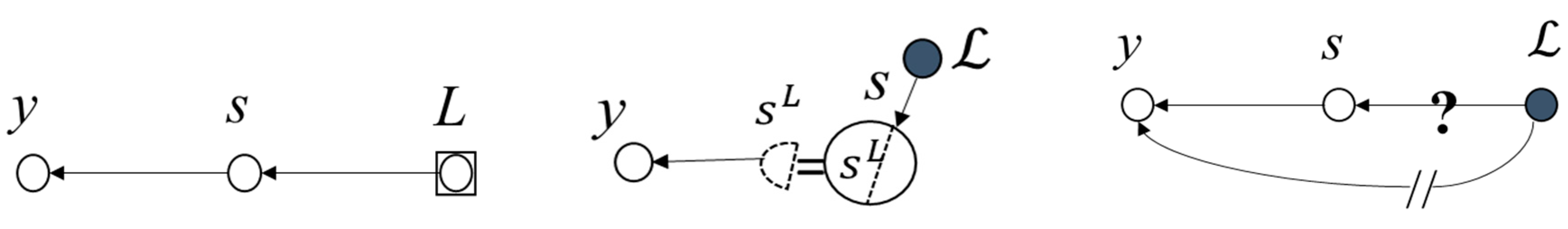
An arguably useful tool to highlight these differences is the directed acyclic graph (DAG), see Cox and Wermuth (1996) and Wermuth and Cox (2011). The left panel of Figure 1 is a DAG of (6). It shows us that, when ATE, i.e., the effect of L forms the focal causal interest, s takes the role of an intermediate variable or a mediator, but when ARTE is the focal interest, L takes the role of a moderator exclusively for s. The second arrow segment, $L\to s$, can be ignored in the latter case, i.e., the case when (6) is reduced into (1). The middle panel is a DAG of (2) + (3).8 This IV-based model is focused on the first arrow segment, since its objective is to reject (1). Hence, the possibility of a causal chain extension is blocked, and L is used to target at producing $s^L\not\approx s$, making ATE of L on y unidentifiable—but neither is ARTE identifiable because s has been significantly modified. Therefore, the definition of ${\beta }_{y{s}^L}$ needs to be modified.

Now, we are in the position of examining the contextual reasons underlying (3) to find out whether the IV-induced modification helps resolve the problems that the approach is intended. Although OVB is stated as the primary problem by AK, it is further compounded, in their justification for the IV route, with two problems—measurement error and selection bias. In view of the current modelling purpose, the concern over measurement error in s is unwarranted because ARTE is not ARTA (average returns to aptitude).9 In other words, measurement error is irrelevant in (1) unless we change its prior stance to explicitly specify s as an imperfect indicator of the latent variable, ‘aptitude’. However, measurement error can provide ${\beta }_{y{s}^L}$ in (3) with a plausible interpretation differently from that of ${\beta }_{ys}$. However, this interpretation would undermine the basic IV-based claim of ${\beta }_{y{s}^L}$ being the consistent estimator of ARTE with respect to s, and openly recognise (1) and (3) as two different models, with (3) effectively yielding ARTA. As for selection bias, the argument extends to the situation where CSL treatment could alter the population composition of educated workers, as compared to that of the pre-treatment population, e.g., through a diluted concentration level of ‘aptitude’ (see Angrist and Pischke 2009, chp. 4). Consequently, the post-treatment schooling effect becomes significantly different from the pre-treatment one due to a change in level of ‘aptitude’ for different years of schooling post-treatment. Two problems hinder this argument. First, there lacks a credible way to verify that a compositional shift, if it has occurred, is adequately reflected by $s^L$ generated via (2). From the perspective of retrospective cross-section data, empirical assessment of the possibility of such a shift entails disaggregation. Specifically, we need to carefully divide the available samples into two parts—an L-treated part versus a CSL unaffected part—so as to investigate whether there exists a parametric difference: ${\beta }_{y{s}_L.Z}\ne {\beta }_{y\widetilde{s_L}.Z}$, where $s_L$ denotes schooling of the L-treated part, and $\widetilde{s_L}$ the treatment unaffected part.10 Even if the inequality is supported by data, the evidence alone is insufficient for rejecting s as a valid conditional variable for y at the aggregate level, e.g., see Engle et al. (1983) and also Qin et al. (2019). Second, the argument assumes a role of L in conflict with its role in the IV treatment of OVB—that the instrument must be unrelated to the omitted variable under the suspicion of causing OVB.

The above analysis not only casts doubt over the explanatory capacity of the IV-based model (3), but also draws our attention to the need to clarify the expected role of L in accordance to our modelling purposes. Clearly, if ATE forms part of our inferential interest, we should not reduce model (6) to (3). Let us turn to this treatment effect. Model (6) tells us that ${\beta }_{yL}={\beta }_{ys}{\beta }_{sL}\ne {\beta }_{ys}$ in general unless ${\beta }_{sL}=1$ can be verified, which is highly unlikely in view of available findings, e.g., see Goldin and Katz (2011). Hence, we should expect that ${\beta }_{yL}\ll {\beta }_{ys}$. However, if ATE is the only parameter of our interest, the chain route of (6) appears a long way round, because ${\beta }_{yL}$ can be estimated directly from:

$$y=a_y+{\beta }_{yL}L+{ϵ}_y.$$

(7)

Unfortunately, this direct route is unfeasible in the samples used by AK and SY because L, a notional variable for CSL, is latent and approximated by various observable indicators, $ℒ$. Consequently, measurement errors are likely to result in ${\beta }_{yℒ}\ne {\beta }_{ys}{\beta }_{sℒ}$, when $ℒ$ is used in (7) instead of L. For instance, SY have identified this kind of defectiveness of CSL indicators, due to their entanglement with regional factors and other controls. On the other hand, a particular case of ${\beta }_{yℒ}\ne {\beta }_{ys}{\beta }_{sℒ}$ signals its associate $ℒ$ being a defective indicator, as it fails to embody the assumed rule of intervention. This failure can be identified via checking ${\beta }_{yℒ.s}\ne 0$ of the following regression:

$$y={\alpha }_y+{\beta }_{ys.ℒ}s+{\beta }_{yℒ.s}ℒ+{\epsilon }_y.$$

(8)

In other words, a test of ${\beta }_{yℒ.s}=0$ using (8) can be exploited as an additional criterion for the purpose of $ℒ$ selection; see Zhang et al. (2017) for implications of measurement error in estimating causal chain models. A DAG illustration of this situation is given in the right panel of Figure 1.

The advantage of the chain route becomes even more evident when the presence of control variables, denoted by Z, is taken into consideration. Although Z is chosen primarily from consideration of $cov\left(sZ\right)\ne 0$, some variables in Z are likely to be correlated with $ℒ$, such as age and regional dummies in the two data sets by AK and SY. The DAGs with Z included are shown in Figure 2. The potential correlation would complicate the estimation of ATE. Extend (6) by Z:

$$\begin{array}{l}y={\alpha }_y+{\beta }_{ys.Z}s+Z^{\prime }{\mathit{\beta }}_{yZ.s}+{\epsilon }_y\\ s={\alpha }_s+{\beta }_{sL}L+{\epsilon }_s\\ Z={\mathit{\alpha }}_Z+L{\mathit{\beta }}_{ZL}+{\mathit{\epsilon }}_Z\end{array}$$

(9)

The corresponding chain representation of the ATE becomes decomposed into two parts:

$${\beta }_{yL}={\beta }_{ys.Z}{\beta }_{sL}+{\mathit{\beta }}_{yZ.s}^{\prime }{\mathit{\beta }}_{ZL}={\beta }_{y{L}_s}+{\beta }_{y{L}_Z}.$$

(10)

Now, only the first component, ${\beta }_{y{L}_s}$, in (10) corresponds to the ATE of L via s. Model (7) is not fit for estimating this parameter.

3. Evaluation of Model Consistency

Section 2 has shown that the IV approach amounts to a model re-specification by replacement of $s$ with $s^L$ as the valid conditional variable, thereby altering the causal interpretation of the coefficient estimates. This re-specification is based on the premise of inconsistency of the OLS model specification relative to its IV counterpart. By exposing the IV approach as a model re-specification, the estimator choice is transposed into one of non-nested model selection, which is testable by use of CV.

In the following, we first replicate results presented by AK and SY, while focusing mainly on SY, to identify conditions under which instrumental validity is achieved and then, by use of CV, reassess these results against the criteria of generalisability and consistency. Since the CSL is latent, it is approximated by observable indicators, $ℒ$. Quarterly birth dummies are chosen by AK (${ℒ}_{AK}$).11 SY, with reference to Acemoglu and Angrist (2001), propose two alternative indicators based on state school and labour law. These indicators capture required years of schooling (${ℒ}_{SY1}$) and compulsory attendance (${ℒ}_{SY2}$).12

Let us inspect the replicate of SY’s results (see Figure 3). The IV-based model specifications appear to lack empirical consistency and robustness relative to their OLS counterpart. ${\beta }^L$ fails to show convergence and standard errors remain large as the sample size increases. Although these findings are common in the literature, their implications are rarely discussed; see Deaton and Cartwright (2018).

Different choices of CSL indicators for generating different $s^L$ result in considerable alteration of the estimation results in SY, as compared to AK. Only in SY, the choice of indicators leads to an apparent success in finding ${\beta }^L\ne \beta$. Further scrutiny through replication of SY’s

Table 1. Sargan and Hausman test for instruments used by SY.

	$\mathbf{T}1\mathbf{A}\left({\mathit{ℒ}}_{\mathit{S}\mathit{Y}1}\right)$				$\mathbf{T}1\mathbf{B}\left({\mathit{ℒ}}_{\mathit{S}\mathit{Y}2}\right)$
White Males	Aged 40–49		Aged 25–54		Aged 40–49		Aged 25–54
	(1)	(2)	(3)	(4)	(1)	(2)	(3)	(4)
$\beta$ (OLS) a	0.073 **	0.073 **	0.063 **	0.063 **	0.073 **	0.073 **	0.063 **	0.063 **
${\beta }^L$ (2SLS) a	0.095 **	−0.020	0.097 **	−0.014	0.142 **	0.092 **	0.140 **	0.086 **
Tests:
Sargan b (p-value)	0.99 (0.6088)	4.65 (0.0977)	17.99 (0.0001)	7.51 (0.0234)	0.64 (0.7271)	0.83 (0.6589)	12.75 (0.0017)	17.57 (0.0002)
Hausman (p-value)	3.80 (0.0512)	9.67 (0.0019)	43.24 (0.0000)	36.32 (0.0000)	16.33 (0.0001)	0.53 (0.4671)	150.29 (0.0000)	3.28 (0.0701)
Fixed effects:
State of birth	Yes	Yes	Yes	Yes	Yes	Yes	Yes	Yes
Year of birth	Yes	Yes	Yes	Yes	Yes	Yes	Yes	Yes
Region x Yob	No	Yes	No	Yes	No	Yes	No	Yes
Additional controls:	None	None	Age quartic, census year	Age quartic, census year	None	None	Age quartic, census year	Age quartic, census year

Notes: Sargan and Hausman added through replication. Source: SY Table 1 and Table A2. ^a Robust and cluster adjusted standard errors are used. ^b Wooldridge’s extension of Sargan’s test of overidentifying restrictions is performed. ** Significant at the 1% level.

and

Table A2. Estimation of $\beta$ via sub-sampling on educational attainment.

	1930–1939 Born				1940–1949 Born
Years of	School		Higher		School		Higher
Schooling	≤12	7–12	13–15	≥13	≤12	7–12	13–15	≥13
SY
$\beta$ (SY)	0.0613 **	0.0587 **	0.0546 **	0.0935 **	0.0612 **	0.0596 **	0.0273 **	0.0641 **
[95% CI] a	[0.0602–0.0625]	[0.0573–0.0601]	[0.0476–0.0615]	[0.0912–0.0957]	[0.0599–0.0624]	[0.0581–0.0611]	[0.0223–0.0322]	[0.0625–0.0657]
${\beta }^L$ (with ${ℒ}_{SY1}$)	0.0942 **	0.0860 *	−0.2577	−0.0218	0.1008 **	0.2072 **	0.4449	0.2292
[95% CI] a	[0.0623–0.1261]	[0.0094–0.1626]	[−0.809–0.2937]	[−0.585–0.541]	[0.0710–0.1305]	[0.0558–0.3586]	[−0.101–0.991]	[−0.124–0.583]
Sargan	0.66 (0.7198)	0.17 (0.9173)	2.43 (0.2963)	5.44 (0.0660)	2.07 (0.3549)	3.59 (0.1661)	8.58 (0.0137)	22.7 (0.0000)
Hausman	4.07 (0.0437)	0.49 (0.4859)	1.43 (0.2325)	0.17 (0.6805)	7.02 (0.0081)	4.63 (0.0315)	2.93 (0.0867)	0.98 (0.3230)
${\beta }^L$ (with ${ℒ}_{SY2}$)	0.1596 **	0.1411 *	−0.5833	0.0831	0.0836 **	0.0671	0.3829	0.0168
[95% CI] a	[0.1182–0.2010]	[0.0193–0.2630]	[−1.76–0.591]	[−0.341–0.5073]	[0.0499–0.1172]	[−0.030–0.164]	[−0.203–0.969]	[−0.267–0.3004]
Sargan	0.21 (0.8990)	11.7 (0.0028)	3.06 (0.2171)	0.56 (0.7563)	7.27 (0.0264)	4.23 (0.1209)	2.33 (0.3123)	9.23 (0.0099)
Hausman	24.6 (0.0000)	1.86 (0.1732)	1.79 (0.1807)	0.002 (0.962)	1.72 (0.1896)	0.02 (0.8799)	1.75 (0.1862)	0.11 (0.7419)
$\beta$ (AK)	0.0565 **	0.0583 **	0.0442 **	0.0591 **	0.0701 **	0.0734 **	0.0153 **	0.0405 **
[95% CI]	[0.0551–0.0578]	[0.0564–0.0601]	[0.0371–0.0515]	[0.0575–0.0607]	[0.0686–0.0716]	[0.0715–0.0753]	[0.0105–0.0201]	[0.0393–0.0416]
${\beta }^L$ (with ${ℒ}_{AK})$	0.0864 **	0.1107 **	0.0295	−0.0446	0.0067	−0.0040	0.0606	0.2612 **
[95% CI]	[0.0357–0.1372]	[0.0288–0.1926]	[−0.309–0.368]	[−0.147–0.058]	[−0.051–0.0641]	[−0.078–0.0696]	[−0.268–0.3888]	[0.1580–0.3644]
Sargan	24.4 (0.7088)	24.2 (0.7217)	33.4 (0.2633)	30.1 (0.4097)	60.8 (0.0005)	59.6 (0.0007)	38.0 (0.1230)	33.5 (0.2587)
Hausman	1.35 (0.2447)	1.60 (0.2054)	0.01 (0.9320)	4.44 (0.0352)	4.84 (0.0279)	4.37 (0.0367)	0.07 (0.7863)	27.5 (0.0000)

Notes: SY data follows model specification (1) Table 1 and Table A2; AK data follows Tables V and VI columns (5) and (6) model specifications. The discrepancy between OLS estimates obtained with SY and AK data sets is due to differences in the construction of the education variable; see Table 3 and discussion. p-values for Sargan and Hausman test in parentheses. ^a Standard errors cluster adjusted. ** Significant at the 1% level. * Significant at the 5% level.

suggests that their CSL indicators are largely invalid instruments. Column (1) in T1B of our Table 1 is the only exception, with no rejection of Sargan’s null of valid overidentifying restrictions and rejection of Hausman’s null of OLS estimator consistency relative to IV. Although the validity of instruments is not rejected for column (2) in T1A of Table 1, the IV estimates remain insignificant.

In contrast to $s$, $s^L$ seems to strongly correlate with covariates such as interaction terms that allow for regional differences in year of birth effects. The inclusion of these interaction terms leads to large changes in ${\beta }^L$, whereas $\beta$ remains virtually invariant; see Figure 3 and columns (2) and (4) of T1A and T1B in Table 1. At the same time, the inclusion of interaction terms invalidates the claim of endogeneity if using ${ℒ}_{SY2}$ indicators and leads to an insignificant ${\beta }^L$ estimate if using ${ℒ}_{SY1}$ indicators. The sensitivity of IV estimates to regional factors has already been pointed out by SY and reiterated by Hoogerheide and van Dijk (2006, Table 5).13 This raises the question of whether ${ℒ}_{SY}$ solely represent the CSL treatment; a potential case of measurement error in these indicators.

The insignificance and empirical inconsistency of ${\beta }^L$, identified in Figure 3 and Table 1, could also be caused by a negligible share of ‘compliers’ in the full sample; a point made by Oreopoulos (2006) in the context of the CSL effect when using minimum years of schooling indicators, and also mentioned by SY as a possible explanation for their results. We hence investigate whether instrumental validity can be achieved when focusing on a sub-sample with a high complier share. We follow AK’s lead and divide the sample by those obtaining 12 years of schooling (school) and those who obtain more than 12 years of schooling (higher). The former sub-sample has a high share of compliers, while the latter sub-sample comprises mainly always takers. Results are reported and discussed in Appendix A. We do not find stronger evidence for instrument validity but make two interesting observations. Firstly, most IV estimates turn insignificant for the ‘higher’ sub-sample, confirming the high share of always takers. Secondly, OLS estimates reveal shrinking ARTE for those with more years of schooling, especially for the 1940–1949 born cohort. This cohort entered the labour market in the early 1980s in the middle of a recession, potentially explaining the low returns to higher education. This effect is concealed in the IV models, given the localness of the CLS instruments.

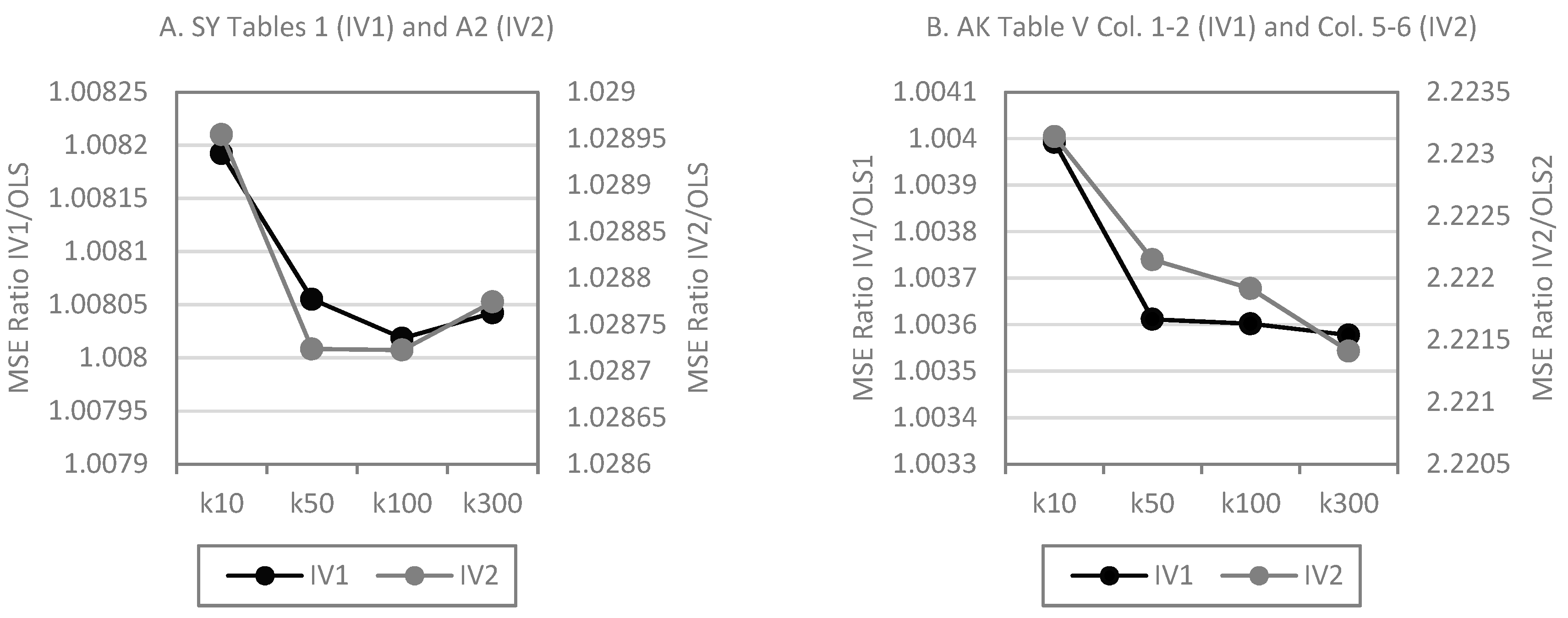
We now turn to CV to formally compare the two non-nested models (1) versus (3). Figure 4 shows that the OLS-based models clearly outperform the IV-based models in generalisability, stability, and consistency, even though the CV experiment presented here does not adjust for degrees of freedom.14 Remarkably, results for AK are close to—or even worse than for—SY, despite the finding of $\beta \approx {\beta }^L$ in AK.

As expected, the MSE decreases as the training sample increases, that is, with increasing k, for both models. However, the IV-based model shows no sign of convergence as training samples grow. When decomposing the MSE into test bias and variance, we find little evidence of asymptotic bias in the OLS estimates; see Figure 5. For the AK case, the IV bias is larger at smaller k and decreases towards no bias at larger k. Given the small bias in general, the large difference in the MSE between the two models clearly stems from a greater variance of the IV model specification, putting the consistency claim of IV into question. While our findings are specific to the CSL case and the chosen instruments, results by Young (2017), who re-evaluates 1359 published IV regressions, suggest that the conclusion drawn from the CV exercise are the norm rather than an exception.

Overall, experimenting with the model design in SY and AK, we find, contrary to what is expected, that the OLS-based model outperforms the IV-based ones in terms of generalisability, stability, and consistency, regardless the choice of CSL indicators.

4. Different Income Effects

Section 3 has provided us with no evidence for $s$ being in invalid causal variable and we now probe into the causal role of $L$. In Section 2, we could distinguish between two income effects: (a) The ARTE effect, ${\beta }_{ys.Z}$, and (b) the CSL effect or ATE of the CSL via schooling, ${\beta }_{y{L}_s}$ as specified in (9).

4.1. Estimating ARTE: ${\beta }_{ys.Z}$

The presentation of varying OLS-based ARTE estimates by AK and SY, despite the use of almost identical samples, indicates problems in the choice of appropriate covariates. Therefore, we proceed with the question of how to specify Z in order to find an empirically adequate specification of (9), which is as parsimonious as possible and can also align the ARTE estimates by AK and SY data, respectively. This is achieved through, firstly, unification of the coding of the education variable and secondly, a parsimonious model specification.

Towards a unification of the education variable, the AK education variable is capped at 17 years to resemble the SY education variable. The unification is found to play a vital role in aligning the ARTE estimates across the two data sets.15 We rely on AK’s division between those born in the 1930s and 1940s, respectively, using observations from the 1980 census. Towards a more parsimonious model, year of birth dummies included by both AK and SY are replaced with quadratic age (age2).16 Regional dummies for individual states are replaced by a single variable distinguishing between four regions for SY and nine regions for AK data (region). Considering a possible regional effect on school quality, variables capturing school quality (pupilt, term, reltwage) suggested by Card and Krueger (1992a, 1992b) are used by SY and included in our model as well.

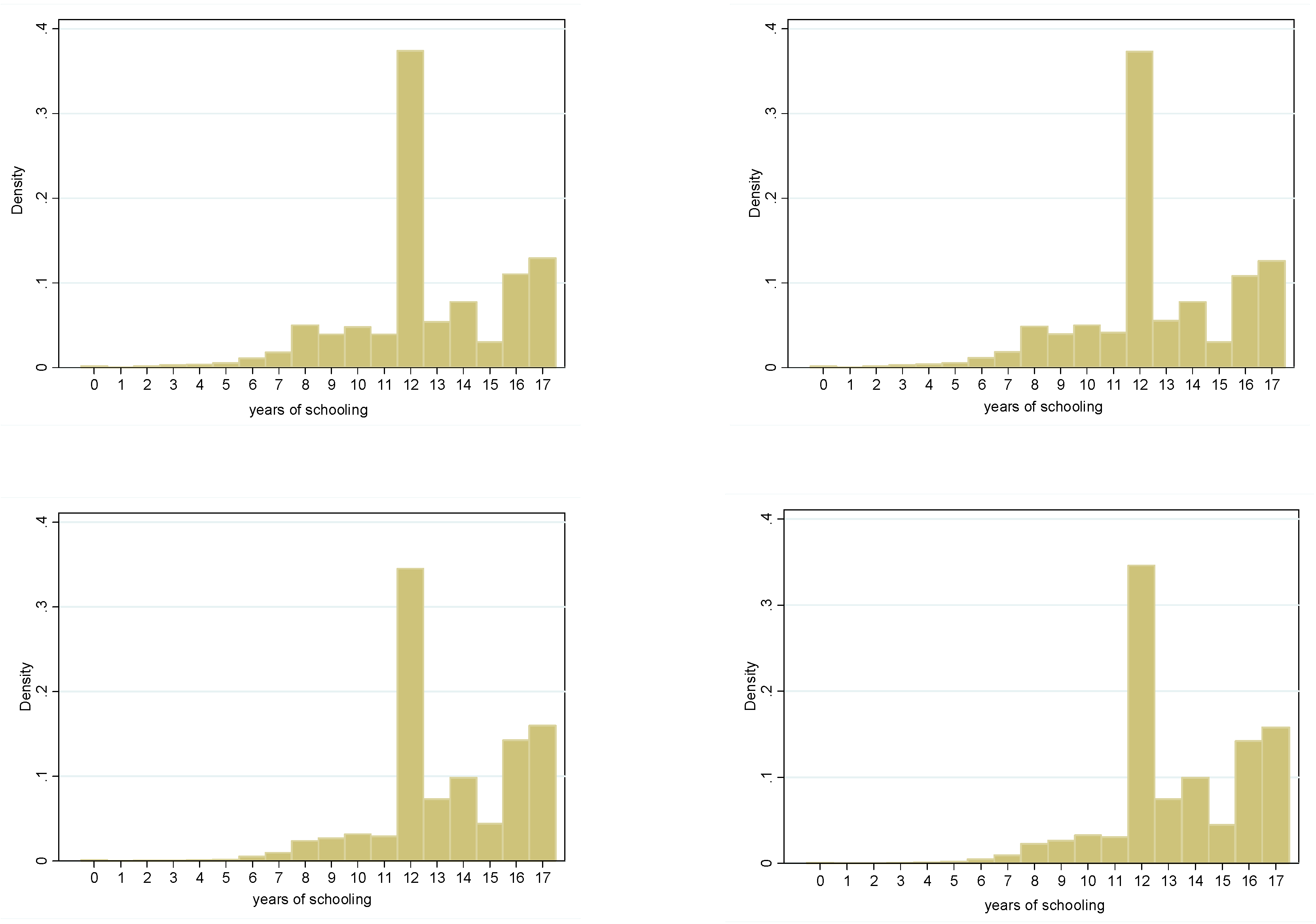
Earlier sub-sample experiments, reported in Appendix A, reveal variation in the ARTE estimates with the level of education. The variation reflects ‘sheepskin effects’, which are well documented phenomena in the literature17 and clearly discernible in the AK and SY data; see Figure A1 and Table A2, Appendix A. A binary variable (uni) is thus added as a classifier for those who obtained a university degree (15 or more years of schooling).

The key results of this model search are reported in

Table 2. Parsimonious specification of (9).

	Original				Alternative
	SY a		AK		SY a		AK
	1930–1939	1940–1949	1930–1939	1940–1949	1930–1939	1940–1949	1930–1939	1940–1949
${\beta }_{ys,Z}$	0.0751 **	0.0622 **	0.0630 **	0.0519 **	0.0600 **	0.0643 **	0.0576 **	0.0648 **
[95% CI]	[0.074–0.077]	[0.061–0.063]	[0.062–0.064]	[0.051–0.053]	[0.058–0.062]	[0.063–0.066]	[0.057–0.059]	[0.064–0.066]
AIC b	714,262.9	1,034,376	594,994.7	858,645.2	705,271.2	1,018,112	594,343.4	858,594.8
Adj.-R2	0.0119	−0.0232	0.1745	0.1354	0.1217	0.0968	0.1761	0.1355
Consist. c	0.0000	0.0000	0.0000	0.0000	0.0000	0.0000	0.0000	0.0000
Zd	age2 age3 age4 yob31-yob39/yob41-yob49 sob1-sob55		ageq, ageq2, race, married, smsa, neweng midatl, enocent, wnocent, soatl, esocent, wsocent, mt, year20-year 28		age2, mar, emp, jail, handcap, pupilt, term, reltwage, uni, region		age2, married, race, smsa, uni, region

Notes: 1980 census, data for SY white male with positive weekly earnings, data for AK male with positive weekly earnings. ^a 95% confidence interval based on cluster adjusted standard errors in SY data. ^b Akaike information criteria. ^c Entner et al. (2012) test for consistency. The row reports the correlation coefficient between ${\epsilon }_y$ in (9) and the residuals from the auxiliary regression, with a value close to 0 confirming consistency. Non-Gaussianity of the residuals was tested before and strongly supported by data. ^d See SY and AK for variable names. ** Significant at the 1% level.

, alongside those from the ‘Original’ models by SY and AK. We refer to our more parsimonious model specifications as ‘Alternative’ in the table. A closer alignment of return to schooling estimates across data sets is achieved with the ‘Alternative’ model specification, which outperforms the ‘Original’ specification in terms of model fit by a margin. OLS estimates point to a relatively constant ${\beta }_{ys.Z}$ of about 0.06 across data sets and cohorts, and our ARTE estimates are roughly in line with findings by Acemoglu and Angrist (2001), who report estimates of 0.061 and 0.075 respectively.

Following the observations in Table 2, we note that the risk of OVB for ${\beta }_{ys.Z}$ comes from inadequately specified $Z$. Hence, we evaluate the choice of $Z$ by use of a simple statistical test of consistency developed by Entner et al. (2012). Recalling the DAG in Figure 2, we can immediately see that in the presence of OVB, that is, missing covariates in $Z$, the residuals ${\epsilon }_y$ in (9) would be statistically dependent on $s$. Entner et al. (2012) exploit this insight by means of a simple two-step algorithm to test the consistency of ${\beta }_{ys.Z}$ against the risk of OVB. In a first step, the key conditional variable $s$ is regressed on the set of covariates Z.18 If residuals of this auxiliary regression are non-Gaussian—Gaussian residuals are a rarity in large cross-sectional data sets—it is tested for being statistically independent between ${\epsilon }_y$ from (9) and the error term of the auxiliary regression in a second step. If independence is confirmed, ${\beta }_{ys.Z}$ is consistent with regards to the choice of covariates Z. The test results are reported in the last row of Table 2. In all cases, consistency is strongly supported by the data.

4.2. Estimating the ATE of the CSL via Schooling: ${\beta }_{y{L}_s}$

Given the potential measurement error in CSL indicators identified by SY and briefly discussed in Section 3, we follow Section 2 and conduct two simple experiments to further test the appropriateness of the indicator choice before continuing with the estimation of ${\beta }_{y{L}_s}$. Since CSL is only binding for school leavers, we would expect the ATE to be insignificant or at least smaller for those with higher education than for those without. Following this reasoning, we estimate the middle equation of (9) using sub-sample groups by educational attainment with the expectation that ${\widehat{\beta }}_{sL}\ne 0$ for School and ${\widehat{\beta }}_{sL}=0$ for Higher.

It is shown in

Table 3. ${\beta }_{sL}$ in (9) via sub-sampling on educational attainment.

	SY						AK
	${\mathit{ℒ}}_{\mathit{S}\mathit{Y}\mathbf{1}}$				${\mathit{ℒ}}_{\mathit{S}\mathit{Y}\mathbf{2}}$				${\mathit{ℒ}}_{\mathit{A}\mathit{K}}$
1930–1939	School		Higher		School		Higher		School		Higher
	Coef.	t-stat a	Coef.	t-stat a	Coef.	t-stat a	Coef.	t-stat a	Coef.	t-stat b	Coef.	t-stat b
${\beta }_{s{ℒ}_1}$	0.38 *	2.50	0.06	0.69	0.18	1.84	−0.1 **	−4.33	−0.1 **	−8.74	0.02	1.17
${\beta }_{s{ℒ}_2}$	0.35 *	2.49	0.07	0.91	−0.02	−0.23	−0.05 *	−1.98	−0.1 **	−8.43	0.05 **	3.10
${\beta }_{s{ℒ}_3}$	0.18	1.25	0.06	0.75	0.39 **	3.99	−0.1 **	−4.27	−0.03 *	−2.39	−0.00	−0.04
	${\mathit{ℒ}}_{\mathit{S}\mathit{Y}\mathbf{1}}$				${\mathit{ℒ}}_{\mathit{S}\mathit{Y}\mathbf{2}}$				${\mathit{ℒ}}_{\mathit{A}\mathit{K}}$
1940–1949	School		Higher		School		Higher		School		Higher
	Coef.	t-stat a	Coef.	t-stat a	Coef.	t-stat a	Coef.	t-stat a	Coef.	t-stat b	Coef.	t-stat b
${\beta }_{s{ℒ}_1}$	0.70 **	11.34	0.13 **	3.47	0.24 **	4.59	−0.05	−1.57	−0.1 **	−9.89	0.04 **	3.71
${\beta }_{s{ℒ}_2}$	0.69 **	10.61	0.25 **	7.63	−0.03	−0.57	0.03	1.00	−0.1 **	−7.82	0.06 **	5.09
${\beta }_{s{ℒ}_3}$	0.42 **	6.25	0.19 **	5.75	0.21 **	3.40	−0.06 *	−2.11	−0.02 *	−2.45	0.03 *	2.25

Notes: 1980 census, data for SY white male with positive weekly earnings, data for AK male with positive weekly earnings. ^a Robust cluster adjusted standard errors. ^b Robust standard errors. ** Significant at the 1% level. * Significant at the 5% level.

that, although ${\widehat{\beta }}_{sL}$ tends to be larger for the School sub-sample than for the Higher sub-sample, none of the indicators confirms the hypothesis of ${\widehat{\beta }}_{sL}=0$ for Higher. Noticeably, the size of those ${\widehat{\beta }}_{sL}\ne 0$ in the first cohort has almost doubled that of the second cohort in the case of SY indicators. This shift appears to reflect a general shift towards more years of education. As seen from

Table A1. Composition of CSL compliers, defectors, and always takers for ${ℒ}_{\mathrm{SY}}.$

Composition of CSL Compliers for SY ${\mathit{ℒ}}_{\mathit{S}\mathit{Y}\mathbf{1}}$
	${\mathit{ℒ}}_{\mathit{S}\mathit{Y}\mathbf{1}}^{\mathbf{1}}=\mathbf{1}$	${\mathit{ℒ}}_{\mathit{S}\mathit{Y}\mathbf{1}}^{\mathbf{2}}=\mathbf{1}$	${\mathit{ℒ}}_{\mathit{S}\mathit{Y}\mathbf{1}}^{\mathbf{3}}=\mathbf{1}$	Total	Years of Schooling	Untreated
1930–1939
Equal	1.37%	5.48%	4.10%	4.11%	${ℒ}_{SY1}^1$: <7	3.75%
Less	2.09%	4.00%	10.19%	6.97%	${ℒ}_{SY1}^2:$ <8	5.88%
More	96.45%	90.57%	85.71%	88.50%	<9	12.28%
N	54,992	116,112	193,730	366,381	N (% of total)	1547 (0.42%)
1940–1949
Equal	0.45%	2.23%	2.90%	2.31%	${ℒ}_{SY1}^1$: <7	3.20%
Less	0.69%	1.55%	5.40%	3.75%	${ℒ}_{SY1}^2:$ <8	5.28%
More	98.86%	96.22%	91.70%	91.71%	${ℒ}_{SY1}^3:$<9	8.87%
N	86,252	112,481	337,979	548,870	N (% of total)	12,158 (2.22%)
Composition of CSL Compliers for SY ${ℒ}_{SY2}$
	${\mathit{ℒ}}_{\mathit{S}\mathit{Y}\mathbf{2}}^{\mathbf{1}}=\mathbf{1}$	${\mathit{ℒ}}_{\mathit{S}\mathit{Y}\mathbf{2}}^{\mathbf{2}}=\mathbf{1}$	${\mathit{ℒ}}_{\mathit{S}\mathit{Y}\mathbf{2}}^{\mathbf{3}}=\mathbf{1}$	Total	Years of Schooling	Untreated
1930–1939
Equal	5.23%	4.11%	5.03%	4.18%	${ℒ}_{SY2}^1$: <8	5.09%
Less	3.65%	10.67%	10.52%	7.44%	${ℒ}_{SY2}^2:$ < 9	10.79%
More	91.20%	85.22%	84.45%	88.38%	${ℒ}_{SY2}^3:$< 10	14.73%
N	116,797	179,705	36,489	366,381	N (% of total)	33,390 (9.11%)
1940–1949
Equal	1.79%	3.00%	3.16%	2.53%	${ℒ}_{SY2}^1$: <8	2.53%
Less	1.38%	5.64%	6.09%	4.30%	${ℒ}_{SY2}^2:$ <9	5.41%
More	96.83%	91.36%	90.74%	93.17%	${ℒ}_{SY2}^3:$<10	8.37%
N	131,875	297,498	82,481	548,870	N (% of total)	37,016 (6.74%)

Notes: ‘N’ is sample size, ‘equal’ is share of those with years of education equal to school law, and ‘less’ years of education and ‘more’ years of education, respectively, for those treated by the respective law. For the untreated group, share of those with less than 7, 8, and 9 years of education among untreated is given. ‘Total’ compares ‘Untreated’ against total of the sample in the equal to the law, less than the law, and more than the law of schooling categories.

(Appendix A), the share of those attaining less or equal the minimum years of schooling is halved in the later cohort.

In a second step, we test whether the rule of intervention ${\beta }_{yℒ.Zs}=0$ holds for the different CSL indicators by estimation of (8) with additional controls Z. In reference to earlier experiments, we conduct the test for the School sub-sample in addition to the full sample estimation. It is shown in

Table 4. Test for the rule of intervention ${\mathsf{\beta }}_{\mathrm{y}ℒ.\mathrm{Zs}}=0$ using (8) extended by $Z.$

	SY a								AK b
	1930–1939				1940–1949				1930–1939		1940–1949
	Full		School		Full		School		${\mathit{ℒ}}_{\mathit{A}\mathit{K}}$		${\mathit{ℒ}}_{\mathit{A}\mathit{K}}$
	${\mathit{ℒ}}_{\mathit{S}\mathit{Y}1}$	${\mathit{ℒ}}_{\mathit{S}\mathit{Y}2}$	${\mathit{ℒ}}_{\mathit{S}\mathit{Y}1}$	${\mathit{ℒ}}_{\mathit{S}\mathit{Y}2}$	${\mathit{ℒ}}_{\mathit{S}\mathit{Y}1}$	${\mathit{ℒ}}_{\mathit{S}\mathit{Y}2}$	${\mathit{ℒ}}_{\mathit{S}\mathit{Y}1}$	${\mathit{ℒ}}_{\mathit{S}\mathit{Y}2}$	Full	School	Full	School
$ℒ1$	−0.001	0.041 **	0.007	0.041 **	0.014	0.041 **	0.007	0.046 **	−0.007 *	−0.008 *	−0.01 **	−0.005
	(0.0133)	(0.0081)	(0.0185)	(0.0100)	(0.0125)	(0.0099)	(0.0146)	(0.0106)	(0.0030)	(0.0039)	(0.0024)	(0.0035)
$ℒ2$	0.011	0.028 **	0.029	0.030 **	0.016	0.047 **	0.020	0.052 **	−0.004	−0.009 *	0.012 **	0.010 **
	(0.0139)	(0.0062)	(0.0189)	(0.0078)	(0.0126)	(0.0081)	(0.0142)	(0.0085)	(0.0030)	(0.0039)	(0.0024)	(0.0035)
$ℒ3$	0.021	0.060 **	0.033	0.063 **	0.033 **	0.078 **	0.031 *	0.082 **	0.001	−0.003	0.012 **	0.017 **
	(0.0144)	(0.0103)	(0.0196)	(0.0113)	(0.0122)	(0.0122)	(0.0140)	(0.0124)	(0.0030)	(0.0038)	(0.0023)	(0.0034)

Notes: 1980 census, data for SY white male with positive weekly earnings, data for AK male with positive weekly earnings. Z as specified in ‘Alternative’ in Table 4. Standard errors reported in parentheses. ^a Robust cluster adjusted standard errors. ^b Robust standard errors. ** Significant at the 1% level. * Significant at the 5% level.

that the condition ${\beta }_{yℒ.Zs}=0$ is validated for SY’s ${ℒ}_{SY1}$ indicator across cohorts and also for AK’s ${ℒ}_{AK}$ indicator for the early born cohort. However, it is violated without exception if using ${ℒ}_{SY2}$ as CSL indicator. Where conditional independence is rejected in Table 4, we have also failed to confirm ${\widehat{\beta }}_{sL}=0$ for the Higher sub-sample in Table 3, and rejected instrument validity in Table 1 and Table A2 Appendix A. In cases like this, we should be cautious with the estimate of ${\beta }_{y{L}_s}$ via the chain representation of (10).

Table 5. Estimated average treatment effect (ATE) of CSL, ${\mathsf{\beta }}_{\mathrm{y}{ℒ}_s}$, using chain models (9) and (10).

	SY a								AK b
	1930–1939				1940–1949				1930–1939		1940–1949
	Full		School		Full		School		Full	School	Full	School
	${\mathit{ℒ}}_{\mathit{S}\mathit{Y}\mathbf{1}}$	${\mathit{ℒ}}_{\mathit{S}\mathit{Y}\mathbf{2}}$	${\mathit{ℒ}}_{\mathit{S}\mathit{Y}\mathbf{1}}$	${\mathit{ℒ}}_{\mathit{S}\mathit{Y}\mathbf{2}}$	${\mathit{ℒ}}_{\mathit{S}\mathit{Y}\mathbf{1}}$	${\mathit{ℒ}}_{\mathit{S}\mathit{Y}\mathbf{2}}$	${\mathit{ℒ}}_{\mathit{S}\mathit{Y}\mathbf{1}}$	${\mathit{ℒ}}_{\mathit{S}\mathit{Y}\mathbf{2}}$	${\mathit{ℒ}}_{\mathit{A}\mathit{K}}$		${\mathit{ℒ}}_{\mathit{A}\mathit{K}}$
$ℒ1$	0.025 **	0.011	0.022 *	0.011 *	0.054 **	0.016 *	0.048 **	0.016 **	−0.009 **	−0.007 **	−0.007 **	−0.007 **
	[12.5]	[2.56]	[6.25]	[3.40]	[88.4]	[6.26]	[125]	[20.8]	[99.2]	[75.2]	[112]	[95.4]
$ℒ2$	0.005	−0.003	0.021 *	−0.001	0.033 **	−0.004	0.045 **	−0.002	−0.006 **	−0.006 **	−0.004 **	−0.005 **
	[0.97]	[0.12]	[6.16]	[0.05]	[35.4]	[0.39]	[107]	[0.32]	[43.4]	[70.0]	[34.3]	[60.4]
$ℒ3$	0.004	0.012	0.011	0.023 **	0.027 **	0.002	0.028 **	0.014 **	−0.002 *	−0.002 *	−0.003 **	−0.002 **
	[0.44]	[3.86]	[1.56]	[15.9]	[20.3]	[0.12]	[37.8]	[11.4]	[4.62]	[5.68]	[15.1]	[6.00]

Notes: 1980 census, data for SY white male with positive weekly earnings, data for AK male with positive weekly earnings. See Table 3 and Table 4 for ${\beta }_{ys.Z}$ and ${\beta }_{sL}$ estimates, respectively. Significance of ${\beta }_{y{ℒ}_s}$ based on χ² statistics estimated following Weesie (1999), reported in brackets. ^a Robust cluster adjusted standard errors. ^b Robust standard errors. ** Significant at the 1% level. * Significant at the 5% level.

provides ${\beta }_{y{L}_s}$ estimated via (10). Where conditional independence is verified, the chain approximation yields significant ATE estimates that confirm our expectation of ${\beta }_{ys.Z}\gg {\beta }_{y{L}_s}$. The estimated ATE almost doubles for the later born cohort from 1–3 to 3–5% using ${ℒ}_{\mathrm{SY}1}$ indicators. The ATE estimates using AK indicators are relatively constant across both sub-samples and cohorts. It should be noted that the negative sign here actually implies a positive ATE, because people born in the first three quarters ${ℒ}_{AK}^1$, ${ℒ}_{AK}^2,$ and ${ℒ}_{AK}^3$ are associated with less years of schooling as compared to those born in the fourth quarter. The CSL effect is strongest for those born in the first quarter and weakens with the second and third quarter born consecutively.

Direct ATE estimates ${\beta }_{yℒ}$ obtained via (7) exceed estimates obtained via chain approximation for the later born cohort; see

Table 6. Estimated ATE of the CSL ${\mathsf{\beta }}_{\mathrm{y}ℒ}$ via (7).

	SY a								AK b
	1930–1939				1940–1949				1930–1939		1940–1949
	Full		School		Full		School		Full	School	Full	School
	${\mathit{ℒ}}_{\mathit{S}\mathit{Y}1}$	${\mathit{ℒ}}_{\mathit{S}\mathit{Y}2}$	${\mathit{ℒ}}_{\mathit{S}\mathit{Y}1}$	${\mathit{ℒ}}_{\mathit{S}\mathit{Y}2}$	${\mathit{ℒ}}_{\mathit{S}\mathit{Y}1}$	${\mathit{ℒ}}_{\mathit{S}\mathit{Y}2}$	${\mathit{ℒ}}_{\mathit{S}\mathit{Y}1}$	${\mathit{ℒ}}_{\mathit{S}\mathit{Y}2}$	${\mathit{ℒ}}_{\mathit{A}\mathit{K}}$		${\mathit{ℒ}}_{\mathit{A}\mathit{K}}$
$ℒ1$	0.033	0.037 **	0.014	0.053 **	0.127 **	0.077 **	0.121 **	0.095 **	−0.014 **	−0.012 **	0.008 **	0.005
	(1.74)	(2.87)	(0.65)	(3.80)	(5.61)	(3.41)	(6.17)	(5.35)	(−4.23)	(−3.10)	(3.02)	(1.43)
$ℒ2$	−0.010	0.022	−0.0004	0.024	0.114 **	0.050 *	0.119 **	0.060 **	−0.009 **	−0.016 **	0.009 **	0.006
	(−0.62)	(1.48)	(−0.02)	(1.69)	(5.74)	(2.28)	(6.60)	(3.40)	(−2.87)	(−3.92	(3.64)	(1.49)
$ℒ3$	0.014	0.071 **	0.006	0.106 **	0.110 **	0.095 **	0.105 **	0.125 **	0.0005	−0.005	0.010 **	0.016 **
	(0.77)	(4.85)	(0.31)	(6.49)	(5.75)	(3.88)	(5.90)	(6.03)	(0.17)	(−1.24)	(4.05)	(4.48)

Notes: 1980 census, data for SY white male with positive weekly earnings, data for AK male with positive weekly earnings. t-statistics reported in parentheses. ^a Robust cluster adjusted standard errors. ^b Robust standard errors. ** Significant at the 1% level. * Significant at the 5% level.

. The effect is indicative of positive indirect CSL effects through control variables Z in later years. Further, chain approximations using SY indicators are much more varied across cohorts than across sub-samples, due to the varying estimates of ${\beta }_{sL}$ in Table 3.

Our finding of a moderate positive ATE of CSL on income (when using labour law indicators) is generally in line with findings reported in the literature; see Acemoglu and Angrist (2001); Lleras-Muney (2002); Oreopoulos (2006); and Goldin and Katz (2011).

5. What Have We Learnt?

Angrist and Pischke (2015, p. 227) discard the Acemoglu and Angrist (2001) study as ‘a failed research design’ and ascribe the failure to inappropriate CSL indicators, while maintaining the IV approach as appropriate. Conceptualising the IV approach as model choice and experimenting with the data sets used by AK and SY, our analysis exposes nescience about the causal model alternation nature of the IV approach to be the root cause of the failure instead.

Primarily, the model choice perspective enables us to transpose the IV-OLS choice into the selection between non-nested models with rival conditional variables. Since consistency is an asymptotic property, this selection can be assisted by CV methods from statistical learning. Our CV experiments show that the OLS-based models outperform the IV-based models in terms of generalisability and stability, regardless the choice of CSL indicators.

Careful examination of the causal implications of the CSL effects on ARTE by causal chain model representation helps us expose several logical flaws in the conceptualisation of IV-based models. First, it is incorrect to refer to ${\beta }_{y{s}^L}$ as a consistent estimate of ARTE when $s^L\not\approx s$. Second, the way in which $s^L$ is generated entangles ARTE with the ATE by CSL in a non-unique manner, reaching deadlock in resolving the ambiguity over the causal interpretation of ${\beta }_{y{s}^L}$. Third, the argument for using IVs to treat measurement errors due to omission of correlated latent variables such as aptitude is unwarranted because ARTE is defined explicitly on education, not aptitude, which entails the specification of ARTA as the parameter of interest.

Experiments with models (9) and (10) show us that relatively robust ${\beta }_{ys.Z}$ estimates are attainable for ARTE, whereas this is not the case with various ATE estimates. The latter finding tells us that measurement error in CSL indicators is indeed a major concern, a result which confirms the common diagnosis of weak and/or inappropriate IVs in the literature. However, our results warn against the IV route as a dead-end in general when using IV to treat a latent variable problem since, in this case, measurement error in IVs is inevitable and also when prior knowledge suggests the need for explicit multivariate model specification with clear differentiation between moderator and mediator effects; see Arlot and Celisse (2010).

Finally, we find clear guidance and reassurance of our approach from the fundamental concepts and theories in statistical learning. In particular, model bias is identified as the primary source of model-based inferential bias. No theoretically postulated model should be taken as globally correct prior to empirical verification, and structural risk minimisation should be regarded as the key task of empirical studies. Applied research should thus be focused on agnostic probably approximately correct (PAC) learning. Once we fully recognise the untenability of the presumption of theoretically postulated models as globally correct, an implicit presumption underlying the IV-choice over OLS, the methodological defects of this estimator-centred research strategy transpire.

References

- Abadie, Alberto, and Matias D. Cattaneo. 2018. Econometric Methods for Program Evaluation. Annual Review of Economics 10: 465–503. [Google Scholar] [CrossRef] [Green Version]
- Acemoglu, Daron, and Joshua D. Angrist. 2001. How Large Are Human Externalities? Evidence from Compulsory Schooling Laws. NBER Macroeconomics Annual 15: 9–74. [Google Scholar] [CrossRef]
- Angrist, Joshua D. 1995. The Economic Returns to Schooling in the West Bank and Gaza Strip. The American Economic Review 85: 1065–87. [Google Scholar]
- Angrist, Joshua D., and Guido W. Imbens. 1995. Two-Stage Least Squares Estimation of Average Causal Effects in Models with Variable Treatment Intensity. Journal of the American Statistical Association 90: 431–42. [Google Scholar] [CrossRef]
- Angrist, Joshua D., Guido W. Imbens, and Donald B. Rubin. 1996. Identification of Causal Effects Using Instrumental Variables. Journal of the American Statistical Association 91: 444–55. [Google Scholar] [CrossRef]
- Angrist, Joshua D., and Alan B. Krueger. 1991. Does Compulsory School Attendance Affect Schooling and Earnings? Quarterly Journal of Economics 106: 979–1014. [Google Scholar] [CrossRef] [Green Version]
- Angrist, Joshua D., and Alan B. Krueger. 1992. The Effect of Age at School Entry on Educational Attainment: An Application of Instrumental Variables with Moments from Two Samples. Journal of the American Statistical Association 87: 328–36. [Google Scholar] [CrossRef]
- Angrist, Joshua D., and Joern-Steffen Pischke. 2015. Mastering ‘Metrics: The Path from Cause to Effect, Princeton. Princeton and Woodstock: Princeton University Press. [Google Scholar]
- Angrist, Joshua D., and Joern-Steffen Pischke. 2009. Mostly Harmless Econometrics: An Empiricist’s Companion, Princeton. Princeton and Woodstock: Princeton University Press. [Google Scholar]
- Arlot, Sylvain, and Alain Celisse. 2010. A Survey of Cross-Validation Procedures for Model Selection. Statistical Surveys 4: 40–79. [Google Scholar] [CrossRef]
- Athey, Susan, and Guido W. Imbens. 2015. Machine Learning Methods for Estimating Heterogeneous Causal Effects, Mimeo. Stanford: Stanford University. [Google Scholar]
- Bolzern, Benjamin, and Martin Huber. 2017. Testing the Validity of the Compulsory Schooling Law Instrument. Economics Letters 159: 23–27. [Google Scholar] [CrossRef]
- Bound, John, and David A. Jaeger. 2000. Do Compulsory School Attendance Laws Alone Explain the Association between Quarter of Birth and Earnings? Worker Well-Being 19: 83–108. [Google Scholar]
- Card, David. 2001. Estimating the Return to Schooling: Progress on Some Persistent Econometric Problems. Econometrica 69: 1127–60. [Google Scholar] [CrossRef]
- Card, David, and Alan B. Krueger. 1992a. Does School Quality Matter? Returns to Education and the Characteristics of Public Schools in the United States. Journal of Political Economy 100: 1–40. [Google Scholar] [CrossRef]
- Card, David, and Alan B. Krueger. 1992b. School Quality and Black-White Relative Earnings: A Direct Assessment. Quarterly Journal of Economics 107: 151–200. [Google Scholar] [CrossRef]
- Carneiro, Pedro, and James J. Heckman. 2002. The Evidence on Credit Constraints in Post-Secondary Schooling. The Economic Journal 112: 989–1018. [Google Scholar] [CrossRef]
- Clark, Damon, and Paco Martorell. 2014. The Signaling Value of a High School Diploma. Journal of Political Economy 122: 282–318. [Google Scholar] [CrossRef] [Green Version]
- Cox, David R., and Nanny Wermuth. 1996. Multivariate Dependencies–Model, Analysis and Interpretation. London: Chapman & Hall. [Google Scholar]
- Cox, David R., and Nanny Wermuth. 2004. Causality: A Statistical View. International Statistical Review 72: 285–305. [Google Scholar] [CrossRef]
- Deaton, Angus. 2009. Instruments of Development: Randomization in the Tropics, and the Search for the Elusive Keys to Economic Development. NBER Working Paper Series; No. 14690. Cambridge: NBER. [Google Scholar]
- Deaton, Angus, and Nancy Cartwright. 2018. Understanding and Misunderstanding Randomized Controlled Trials. Social Science & Medicine 210: 2–21. [Google Scholar]
- Durbin, James. 1954. Errors in Variables. Review of the International Statistical Institute 22: 23–32. [Google Scholar] [CrossRef]
- Engle, Robert F., David F. Hendry, and Jean-Francois Richard. 1983. Exogeneity. Econometrica 51: 277–304. [Google Scholar] [CrossRef]
- Entner, Doris, Patrik O. Hoyer, and Peter Spirtes. 2012. Statistical Test for Consistent Estimation of Causal Effects in Linear Non-Gaussian Models. Paper presented at the 15th International Conference on Artificial Intelligence and Statistics (AISTATS) 2012, La Palma, Canary Islands, Spain, April 21–23. [Google Scholar]
- Goldin, Claudia. 1998. America’s graduation from high school: The evolution and spread of secondary schooling in the twentieth century. Journal of Economic History 58: 345–74. [Google Scholar] [CrossRef]
- Goldin, Claudia, and Lawrence F. Katz. 2000. Education and Income in the Early 20th Century: Evidence from the Prairies. The Journal of Economic History 60: 782–818. [Google Scholar] [CrossRef]
- Goldin, Claudia, and Lawrence F. Katz. 2007. Long-Run Changes in the U.S. Wage Structure: Narrowing, Widening, Polarizing. NBER Working Paper Series; No. 13568. Cambridge: NBER. [Google Scholar]
- Goldin, Claudia, and Lawrence F. Katz. 2011. Mass Secondary Schooling and the State: The Role of State Compulsion in the High School Movement. In Understanding Long Run Economic Growth. Edited by Dora Costa and Naomi Lamoreaux. Chicago: University of Chicago Press, pp. 275–310. [Google Scholar]
- Harmon, Colm, Hessel Oosterbeek, and Ian Walker. 2003. The Returns to Education: Microeconomics. Journal of Economic Surveys 17: 115–55. [Google Scholar] [CrossRef]
- Heckman, James J., and Sergio Urzua. 2009. Comparing IV with Structural Models: What Simple IV Can and Cannot Identify. NBER Working Paper Series; No. 14706. Cambridge: NBER. [Google Scholar]
- Hoogerheide, Lennart, and Herman K. van Dijk. 2006. A Reconsideration of the Angrist-Krueger Analysis on Returns to Education. Econometric Institute Report EI 2006-15. Rotterdam: Econometric Institute. [Google Scholar]
- Imbens, Guido W. 2010. Better LATE Than Nothing: Some Comments on Deaton (2009) and Heckman and Urzua (2009). Journal of Economic Literature 48: 399–423. [Google Scholar] [CrossRef]
- Kolesár, Michal, Raj Chetty, John Friedman, Edward Glaeser, and Guido W. Imbens. 2015. Identification and Inference with Many Invalid Instruments. Journal of Business & Economic Statistics 33: 474–84. [Google Scholar]
- Lleras-Muney, Adriana. 2002. Were Compulsory Attendance and Child Labor Laws Effective? An Analysis from 1915 to 1939. The Journal of Law and Economics 45: 401–35. [Google Scholar] [CrossRef]
- Ludwig, Jens, Greg J. Duncan, Lisa A. Gennetian, Lawrence F. Katz, Roland C. Kessler, Jeffrey R. Kling, and Lisa Sanbonmatsu. 2013. Long-Term Neighborhood Effect on Low-Income Families: Evidence from Moving to Opportunity. American Economic Review 103: 226–31. [Google Scholar] [CrossRef]
- Ludwig, Jens, Greg J. Duncan, Lisa A. Gennetian, Lawrence F. Katz, Roland C. Kessler, Jeffrey R. Kling, and Lisa Sanbonmatsu. 2012. Neighborhood Effects on the Long-Term Well-Being of Low-Income Adults. Science 337: 1505–10. [Google Scholar] [CrossRef]
- Mukherjee, Sayan, Partha Niyogi, Tomaso Poggio, and Ryan Rifkin. 2006. Learning Theory: Stability is Sufficient for Generalization and Necessary and Sufficient for Consistency of Empirical Risk Minimization. Advances in Computational Mathematics 25: 161–93. [Google Scholar] [CrossRef]
- Murphy, Kevin M., and Finis Welch. 1992. The Structure of Wages. The Quarterly Journal of Economics 107: 285–326. [Google Scholar] [CrossRef]
- Oreopoulos, Philip. 2006. Estimating Average and Local Average Treatment Effects of Education when Compulsory Schooling Laws Really Matter. American Economic Review 96: 152–75. [Google Scholar] [CrossRef]
- Pearl, Judea. 2009. Causality: Models, Reasoning, and Inference, 2nd ed. Cambridge: Cambridge University Press. [Google Scholar]
- Qin, Duo. 2015. Resurgence of the Endogeneity-Backed Instrumental Variable Methods. Economics: The Open-Access, Open-Assessment E-Journal 9: 1–35. [Google Scholar] [CrossRef]
- Qin, Duo. 2018. Let’s Take the Bias Out of Econometrics. Journal of Economic Methodology 26: 81–98. [Google Scholar] [CrossRef]
- Qin, Duo, Sophie van Huellen, Raghda Elshafie, Yimeng Liu, and Thanos Moraitis. 2019. A Principled Approach to Assessing Missing-Wage Induced Selection Bias. SOAS Department of Economics Working Paper Series; No. 216. London: SOAS. [Google Scholar]
- Shalev-Shwartz, Shai, and Shai Ben-David. 2014. Understanding Machine Learning: From Theory to Algorithms. Cambridge: Cambridge University Press. [Google Scholar]
- Shalev-Shwartz, Shai, Ohad Shamir, Nathan Srebro, and Karthik Sridharan. 2010. Learnability, Stability and Uniform Consistency. Journal of Machine Learning Research 11: 2635–70. [Google Scholar]
- Stephens, Melvin, Jr., and Dou-Yan Yang. 2014. Compulsory Education and the Benefits of Schooling. American Economic Review 104: 1777–92. [Google Scholar] [CrossRef]
- Stock, James H., Jonathan H. Wright, and Motohiro Yogo. 2002. A Survey of Weak Instruments and Weak Identification in Generalized Method of Moments. Journal of Business & Economic Statistics 20: 518–29. [Google Scholar]
- Trostel, Philip. A. 2005. Nonlinearity in the Return to Education. Journal of Applied Economics 8: 191–202. [Google Scholar] [CrossRef] [Green Version]
- Weesie, Jeroen. 1999. Seemingly Unrelated Estimation and The Cluster-adjusted Sandwich Estimator. Stata Technical Bulletin 52: 34–47, Reprinted in Stata Technical Bulletin Reprints 9: 231–48. [Google Scholar]
- Wermuth, Nanny, and David R. Cox. 2011. Graphical Markov Models: Overview. In International Encyclopedia of Social and Behavioral Sciences, 2nd ed. Edited by Wright James. New York: Elesevier, pp. 341–50. [Google Scholar]
- Young, Alwyn. 2017. Consistency without Inference: Instrumental Variables in Practical Application, Mimeo. London: London School of Economics. [Google Scholar]
- Zhang, Kun, Mingming Gong, Joseph Ramsey, Kayhan Batmanghelich, Peter Spirtes, and Clark Glymour. 2017. Causal Discovery in the Presence of Measurement Error: Identifiability Conditions. Paper presented at the UAI 2017 Workshop on Causality, Sydney, Australia, August 11–15. [Google Scholar]
- Zhang, Yongli, and Yuhong Yang. 2015. Cross-Validation for Selecting a Model Selection Procedure. Journal of Econometrics 187: 95–112. [Google Scholar] [CrossRef]