A Combination Method for Averaging OLS and GLS Estimators ^†

Abstract

To avoid the risk of misspecification between homoscedastic and heteroscedastic models, we propose a combination method based on ordinary least-squares (OLS) and generalized least-squares (GLS) model-averaging estimators. To select optimal weights for the combination, we suggest two information criteria and propose feasible versions that work even when the variance-covariance matrix is unknown. The optimality of the method is proven under some regularity conditions. The results of a Monte Carlo simulation demonstrate that the method is adaptive in the sense that it achieves almost the same estimation accuracy as if the homoscedasticity or heteroscedasticity of the error term were known.

1. Introduction

Model averaging has been developed as an alternative to model selection. In many situations, model-averaging methods perform better than alternative model-selection methods. The main reason for this is that model selection delivers a pretest estimator that has inferior properties, and its use can be harmful (see Danilov and Magnus, 2004). Yuan and Yang (2005) provided a detailed discussion on the choice between model averaging and model selection. As one of the pioneers of frequentist model averaging, Hansen (2007) proposed Mallows model averaging (MMA) based on the ordinary least-squares (OLS) estimator for linear regression models with homoscedastic errors. Wan et al. (2010) extended the results for non-nested models with homoscedastic errors. Zhao et al. (2018) is the most recent work in this area. For linear regression models with heteroscedastic errors, Hansen and Racine (2012), Liu and Okui (2013) and Zhang et al. (2013, 2015) proposed model averaging methods that are still based on the OLS estimator, while Liu et al. (2016) proposed a method based on the generalized least squares estimator (GLS). They demonstrated that their methods are optimal in the sense of Li (1987) for homoscedastic or heteroscedastic models. For model averaging in big datasets, Xie (2017) proposed the use of model screening (before averaging) in order to deal with the large number of candidate models/regressors.

However, all previous papers assumed that it was known whether the errors of the true data-generating process are homoscedastic or heteroscedastic. Due to this assumption, the previous averaging methods were based only on estimators constructed using the same estimation method, either OLS or GLS estimators (with different regressor sets). This assumption can be unrealistic in empirical applications. Usually, researchers do not know the structure of the error term; therefore, this assumption leads to possible misspecification. A natural solution is to combine OLS and GLS estimators. Combinations of different methods are routinely used in the applied forecast combination literature. In a recent forecasting competition that included 100,000 series, Makridakis et al. (2018) found that, out of the 17 most accurate methods, 12 were combinations. All combinations used different models/methods varying from simple exponential smoothing models to sophisticated machine-learning algorithms.

We propose a combination method based on OLS and GLS estimators to reduce the risk of misspecification between homoscedastic and heteroscedastic linear models. More precisely, the proposed estimator is a weighted average of mixtures of OLS and GLS estimators. The OLS mixture is constructed using the MMA of Hansen (2007) or the heteroscedasticity-robust Cp(HRCp) model averaging of Liu and Okui (2013). The GLS mixture is constructed using the GLS model averaging (GLSMA) of Liu et al. (2016).

We propose the use of two criteria, MMA-GLSMA and HRCp-GLSMA, to choose the weight vector for combining estimators. The optimality of the chosen weight vector in the sense of Li (1987) is investigated. Our method works in situations with an unknown variance-covariance matrix of the error term if an estimate based on the nonparametric method k-nearest neighbours (k-NN) is used. The results of the simulation experiments show that our combination method is adaptive in the sense that it can achieve almost the same estimation accuracy as if the homoscedasticity or heteroscedasticity of the error term was known.

The rest of the paper is organized as follows: In Section 2, we describe the theoretical setup and introduce the new combination method with the criteria for choosing the weight vector. In Section 3, we investigate the optimality of the proposed criteria. Section 4 presents the results of the Monte Carlo simulations. Section 5 concludes the paper, and all proofs are provided in the Appendix A.

2. Method

Suppose that we have an independent random sample of $(y_i,x_i)$ for $i=1,\cdots ,n$, where $x_i={(x_{i1},x_{i2},\cdots ,)}^{\prime }$ is a countably infinite real-valued vector and $y_i$ is a real-valued scalar random variable generated from an infinite dimensional linear regression model:

$$\begin{array}{ccc}\hfill y_i& =& {\mu }_i+e_i,\hfill \end{array}$$

where:

$$\begin{array}{ccc}\hfill {\mu }_i& =& \sum _{j=1}^{\infty }{\theta }_j{x}_{ij},\hfill \end{array}$$

$e_i$ is an unobserved error term that can be homoscedastic or heteroscedastic with $E\left(e_i\right|x_i)=0$, $E\left(e_i^2\right)={\sigma }^2$ and $E\left(e_i^2\right|x_i)={\sigma }_i^2$ and ${\theta }_j$ for $j=1,2,\cdots$ are unknown parameters. We also define $X\equiv \left(x_1,\cdots ,x_n\right)$, $Y\equiv {\left(y_1,\cdots ,y_n\right)}^{{}^{\prime }}$, $\mu \equiv {\left({\mu }_1,\cdots ,{\mu }_n\right)}^{{}^{\prime }}$, $e\equiv {\left(e_1,\cdots ,e_n\right)}^{{}^{\prime }}$ and denote the variance-covariance matrix as $\Omega \equiv E\left(e{e}^{{}^{\prime }}|X\right)=diag({\sigma }_1^2,\cdots ,{\sigma }_n^2)$. We state the theoretical results considering the distributions conditional on X and omit all notations for those conditional on X hereafter.

2.1. Infeasible Combination Estimator and Information Criteria

Suppose $\Omega$ is known; we have a candidate set of $M_1$ linear models with different numbers of independent variables for OLS estimation and a candidate set of $M_2$ linear models with different numbers of independent variables for GLS estimation. Then, we can obtain a set of OLS estimates ${\widehat{\mu }}_m^{ols}\equiv P_{m}Y$ for $m=1,\cdots ,M_1$ and a set of GLS estimates ${\widehat{\mu }}_m^{gls}\equiv G_{m}Y$ for $m=1,\cdots ,M_2$. Therein, $P_m=X_m{\left(X_m^{\prime }{X}_m\right)}^{-1}{X}_m^{\prime }$ is the projection matrix of the $m^{\mathrm{th}}$ regression model for OLS with $m=1,\cdots ,M_1$, and $G_m\equiv X_m{\left(X_m^{\prime }{\Omega }^{-1}{X}_m\right)}^{-1}{X}_m^{\prime }{\Omega }^{-1}$ with $X_m$ being the independent variable matrix of the $m^{\mathrm{th}}$ regression model for GLS with $m=1,\cdots ,M_2$. In this paper, we only consider the situation with nested models for both OLS and GLS estimators. This means that the $m^{\mathrm{th}}$ model is nested in the ${(m+1)}^{\mathrm{th}}$ model. Theoretical results may be extended to non-nested candidate models using the approach of Wan et al. (2010). Moreover, $M_1$ and $M_2$ can be fixed or go to infinity when the sample size n is increasing.

Based on those OLS and GLS estimates, we construct a combination estimator as follows:

$$\begin{array}{cc}\hfill \widehat{\mu }\left(W\right)& =\sum _{m=1}^{M_1}{w}_m^{ols}{\widehat{\mu }}_m^{ols}+\sum _{m=1}^{M_2}{w}_m^{gls}{\widehat{\mu }}_m^{gls},\hfill \\ \hfill & \equiv {\widehat{\mu }}_{ols}\left(W_1\right)+{\widehat{\mu }}_{gls}\left(W_2\right)\hfill \end{array}$$

where $W=\left(W_1^{{}^{\prime }},W_2^{{}^{\prime }}\right)={\left(w_1^{ols},\cdots ,w_{M_1}^{ols},w_1^{gls},\cdots ,w_{M_2}^{gls}\right)}^{{}^{\prime }}$ belongs to:

$$\mathcal{H}=\left\{W\left|W\in {\left[0,1\right]}^M,I^{\prime }W=1\right.\right\},$$

where $M=M_1+M_2$ and I denote a $M\times 1$ vector having all elements equal to one.

In order to reduce the risk of the combination-estimation method proposed above, we need to select a suitable weight vector. To do that, in this subsection, we propose two versions, MMA-GLSMA and HRCp-GLSMA, with infeasible criteria. In the next subsection, we provide their feasible counterparts for the situation with unknown $\Omega$ values.

HRCp-GLSMA: The first information criterion for selecting a weight vector is defined as:

$$\begin{array}{ccc}\hfill {\overline{C}}_n\left(W\right)& =& s_1^2\left\{{∥Y-{\widehat{\mu }}_{ols}\left(W_1^{*}\right)∥}^2+2tr\left(P\left(W_1^{*}\right)\Omega \right)\right\}\hfill \end{array}$$

(1)

$$\begin{array}{c}+s_2^2\left\{{∥Y-{\widehat{\mu }}_{gls}\left(W_2^{*}\right)∥}^2+2tr\left(G\left(W_2^{*}\right)\Omega \right)\right\}\hfill \end{array}$$

(2)

$$\begin{array}{c}+2s_1{s}_2\left\{{\left(Y-{\widehat{\mu }}_{ols}\left(W_1^{*}\right)\right)}^{{}^{\prime }}\left(Y-{\widehat{\mu }}_{gls}\left(W_2^{*}\right)\right)\right.\hfill \end{array}$$

(3)

$$\begin{array}{c}\left.+tr\left(P\left(W_1^{*}\right)\Omega \right)+tr\left(G\left(W_2^{*}\right)\Omega \right)-e^{{}^{\prime }}e\right\},\hfill \end{array}$$

(4)

where $s_1\equiv {\sum }_{m=1}^{M_1}{w}_m^{ols}$, $s_2\equiv {\sum }_{m=1}^{M_2}{w}_m^{gls}$, $W_1^{*}\equiv W_1/s_1$, $W_2^{*}\equiv W_2/s_2$, $P\left(W_1^{*}\right)\equiv {\sum }_{m=1}^{M_1}{w}_m^{ols}{P}_m$ and $G\left(W_2^{*}\right)\equiv {\sum }_{m=1}^{M_2}{w}_m^{gls}{G}_m$.

Note that:

$$\begin{array}{cc}\hfill {\overline{C}}_n\left(W\right)& =s_1^{2}HR{C}_p\left(W_1^{*}\right)+s_2^2{C}_{I_n}\left(W_2^{*}\right)\hfill \\ \hfill & +2s_1{s}_2\left\{{\left(Y-{\widehat{\mu }}_{ols}\left(W_1^{*}\right)\right)}^{{}^{\prime }}\left(Y-{\widehat{\mu }}_{gls}\left(W_2^{*}\right)\right)\right.\hfill \\ \hfill & \left.+tr\left(P\left(W_1^{*}\right)\Omega \right)+tr\left(G\left(W_2^{*}\right)\Omega \right)-e^{{}^{\prime }}e\right\},\hfill \end{array}$$

where $HR{C}_p\left(W_1^{*}\right)={∥Y-{\widehat{\mu }}_{ols}\left(W_1^{*}\right)∥}^2+2tr\left(P\left(W_1^{*}\right)\Omega \right)$ is the HRCp model-averaging criterion proposed by Liu and Okui (2013) with the weight vector $W_1^{*}$ and $C_{I_n}\left(W_2^{*}\right)={∥Y-{\widehat{\mu }}_{gls}\left(W_2^{*}\right)∥}^2+2tr\left(G\left(W_2^{*}\right)\Omega \right)$ is a GLSMA information criterion proposed by Liu et al. (2016) with the weight vector $W_2^{*}$. $\overline{C}$ can be regarded as a combination of the HRCp and the GLSMA. Hence, we call $\overline{C}$ the HRCp-GLSMA-type criterion.

MMA-GLSMA: Second, we propose an MMA-GLSMA-type criterion for weight selection. The infeasible MMA-GLSMA-type criterion is defined as follows:

$$\begin{array}{ccc}\hfill {\tilde{C}}_n\left(W\right)& =& s_1^2{C}_{MMA}\left(W_1^{*}\right)+s_2^2{C}_{I_n}\left(W_2^{*}\right)\hfill \\ & & +2s_1{s}_2\left\{{\left(Y-{\widehat{\mu }}_{ols}\left(W_1^{*}\right)\right)}^{{}^{\prime }}\left(Y-{\widehat{\mu }}_{gls}\left(W_2^{*}\right)\right)\right.\hfill \\ & & \left.+{\sigma }^{2}tr\left(P\left(W_1^{*}\right)\right)+tr\left(G\left(W_2^{*}\right)\Omega \right)-e^{{}^{\prime }}e\right\},\hfill \end{array}$$

where $C_{MMA}\left(W_1^{*}\right)={∥Y-{\widehat{\mu }}_{ols}\left(W_1^{*}\right)∥}^2+2{\sigma }^{2}tr\left(P\left(W_1^{*}\right)\right)$ is the MMA criterion proposed by Hansen (2007) with the weight vector $W_1^{*}$.

Suppose the variance-covariance matrix $\Omega$ is known; we can then choose the weight by minimizing the criteria ${\overline{C}}_n$ or ${\tilde{C}}_n$, as follows:

$$\overline{W}=arg\underset{W\in H}{min}{\overline{C}}_n$$

or

$$\tilde{W}=arg\underset{W\in H}{min}{\tilde{C}}_n.$$

However, since the variance-covariance matrix $\Omega$ is unknown, $\overline{W}$ and $\tilde{W}$ are infeasible.

2.2. Feasible Combination Estimator and Information Criteria

For a situation with unknown variance, a feasible combination estimator can be constructed using feasible GLS (FGLS) estimators. FGLS estimators and the feasible combination estimator are defined below:

$$\begin{array}{cc}\hfill {\widehat{\mu }}^F\left(W\right)& =\sum _{m=1}^{M_1}{w}_m^{ols}{\widehat{\mu }}_m^{ols}+\sum _{m=1}^{M_2}{w}_m^{gls}{\widehat{\mu }}_m^{fgls},\hfill \\ \hfill & \equiv {\widehat{\mu }}_{ols}\left(W_1\right)+{\widehat{\mu }}_{fgls}\left(W_2\right)\hfill \end{array}$$

where the FGLS estimator is ${\widehat{\mu }}_m^{fgls}\equiv X_m{\left(X_m^{\prime }{\widehat{\Omega }}^{-1}{X}_m\right)}^{-1}{X}_m^{\prime }{\widehat{\Omega }}^{-1}Y$. Therein, the estimator $\widehat{\Omega }$ is based on the k-NN estimator ${\check{{\sigma }_i}}^2$ of Liu et al. (2016).

We propose two feasible counterparts of ${\overline{C}}_n$ and ${\tilde{C}}_n$. The feasible HRCp-GLSMA-type criterion ${\overline{C}}_n^F$ is defined as:

$$\begin{array}{c}\hfill \begin{array}{ccc}{\overline{C}}_n^F\left(W\right)& =& s_1^2\left\{{∥Y-{\widehat{\mu }}_{ols}\left(W_1^{*}\right)∥}^2+2\sum _{i=1}^n{\widehat{e}}_i^2{p}_{ii}\left(W_1^{*}\right)\right\}\hfill \\ & & +s_2^2\left\{{∥Y-{\widehat{\mu }}_{fgls}\left(W_2^{*}\right)∥}^2+2tr\left(G^F\left(W_2^{*}\right)\widehat{\Omega }\right)\right\}\hfill \\ & & +2s_1{s}_2\left\{{\left(Y-{\widehat{\mu }}_{ols}\left(W_1^{*}\right)\right)}^{{}^{\prime }}\left(Y-{\widehat{\mu }}_{fgls}\left(W_2^{*}\right)\right)\right.\hfill \\ & & \left.+tr\left(P\left(W_1^{*}\right)\widehat{\Omega }\right)+tr\left(G^F\left(W_2^{*}\right)\widehat{\Omega }\right)-{\widehat{e}}^{{}^{\prime }}\widehat{e}\right\},\hfill \end{array}\end{array}$$

(5)

and the feasible MMA-GLSMA-type criterion ${\tilde{C}}_n^F$ is defined as:

$$\begin{array}{c}\hfill \begin{array}{ccc}{\tilde{C}}_n^F\left(W\right)& =& s_1^2\left\{{∥Y-{\widehat{\mu }}_{ols}\left(W_1^{*}\right)∥}^2+2{\widehat{\sigma }}^{2}tr\left(P\left(W_1^{*}\right)\right)\right\}\hfill \\ & & +s_2^2\left\{{∥Y-{\widehat{\mu }}_{fgls}\left(W_2^{*}\right)∥}^2+2tr\left(G^F\left(W_2^{*}\right)\widehat{\Omega }\right)\right\}\hfill \\ & & +2s_1{s}_2\left\{{\left(Y-{\widehat{\mu }}_{ols}\left(W_1^{*}\right)\right)}^{{}^{\prime }}\left(Y-{\widehat{\mu }}_{fgls}\left(W_2^{*}\right)\right)\right.\hfill \\ & & \left.+{\widehat{\sigma }}^{2}tr\left(P\left(W_1^{*}\right)\right)+tr\left(G^F\left(W_2^{*}\right)\widehat{\Omega }\right)-{\widehat{e}}^{{}^{\prime }}\widehat{e}\right\},\hfill \end{array}\end{array}$$

(6)

where ${\widehat{e}}_i$ denotes the $i^{\mathrm{th}}$ element of $\widehat{e}\equiv \sqrt{n/\left(n-k_L\right)}$$\left(I-P_L\right)Y$ with $k_L$ denoting the number of independent variables in the largest OLS model:

$$G^F\left(W_2^{*}\right)=\sum _{m=1}^{M_2}{w}_m^{gls}{X}_m{\left(X_m^{\prime }\widehat{\Omega }{X}_m\right)}^{-1}{X}_m^{\prime }{\widehat{\Omega }}^{-1}.$$

$P_L$ denotes the projection matrix of that model, and $p_{ii}$ denotes the $i^{\mathrm{th}}$ diagonal element of $P\left(W_1^{*}\right)$. $\tilde{e}\equiv \left(I-P_L\right)Y$, while ${\widehat{\sigma }}^2\equiv {\left(n-k_L\right)}^{-1}{\tilde{e}}^{{}^{\prime }}\tilde{e}$ is defined as one of the estimators suggested by Hansen (2007). $\widehat{\Omega }$ is calculated by plugging in the k-NN estimator ${\check{{\sigma }_i}}^2$ used in Liu et al. (2016).

3. Properties of the Criteria

The following lemma demonstrates the significant fact that the two infeasible criteria proposed above are unbiased estimates of the risk function $R\left(W\right)\equiv E\left(L\left(W\right)\right)$ plus a constant; $L\left(W\right)\equiv {∥\mu -\widehat{\mu }\left(W\right)∥}^2$ is the loss function.

Lemma 1.

For any real-valued vector W, $E\left({\overline{C}}_n\left(W\right)\right)=R\left(W\right)+c_1$ and $E\left({\tilde{C}}_n\left(W\right)\right)=R\left(W\right)+c_2$, where $c_1$ and $c_2$ are constants.

Another useful property is that all criteria are asymptotically optimal in the sense of Li (1987). Proofs of the asymptotic optimality for all of the above-mentioned criteria can be performed by extending the proofs of Hansen (2007); Liu and Okui (2013); Liu et al. (2016). As an example, we demonstrate the optimality of the feasible MMA-GLSMA case method with the nonparametric estimator of $\Omega$ used in Liu et al. (2016).

To do that, we define the feasible loss function and the risk function as follows:

$$\begin{array}{cc}\hfill L^F\left(W\right)& \equiv {∥\mu -{\widehat{\mu }}^F\left(W\right)∥}^2\hfill \\ \hfill & ={({\widehat{\mu }}^F\left(W\right)-\mu )}^{\prime }({\widehat{\mu }}^F\left(W\right)-\mu ).\hfill \end{array}$$

We employ some notations and assumptions from Liu et al. (2016), reproduced in the Appendix, and add the following additional assumption:

Assumption 1.

As $n\to \infty$ and $k_l\to \infty$, $\left(k_l+k_l\sqrt{{\sum }_{j=1}^n{b}_{lj}^2}\right)/{\xi }_n\to 0$, where ${\xi }_n\equiv {inf}_{W\in {\mathcal{H}}_n\left(N\right)}R\left(W\right)$, $k_l$ is the number of regressors used in the regression model for the k-NN estimator and $b_{li}$ denotes the approximation error of that model.

Assumption 1’ guarantees that when the number of regressors used in the regression model (adjusted with the approximation errors of that model) increases with the sample size n, it increases at a rate slower than the lower bound of the risk across all possible weights. In practice, this assumption requires us to moderate the increase in the number of regressors $k_l$ (relative to the sample size) to reduce the approximation errors.

Following Hansen (2007), we restrict the elements of the weighting vector to belong to set ${\mathcal{H}}_M\left(N\right)\equiv \{0,1/N,2/N,\cdots ,1\}$ for some integer $N<\infty$.

Theorem 1.

Under Assumption 1’ and Assumptions 1–3, 6, and 10–14 of Liu et al. (2016), as $n\to \infty$, $k_l\to \infty$, $\kappa \to \infty$ and $k_L/\sqrt{n}\to 0$, we have:

$$\begin{array}{c}\hfill \frac{L^F\left(\tilde{W}\right)}{{inf}_{W\in {\mathcal{H}}_M\left(N\right)}L\left(W\right)}{\to }_{p}1,\end{array}$$

where $\tilde{W}=arg{min}_{W\in {\mathcal{H}}_M\left(N\right)}{\tilde{C}}_n^F\left(W\right)$.

In other words, as the sample size increases, our method can achieve the infimum of the loss.

4. Simulation Study

To investigate the finite sample performance of the proposed MMA-GLSMA and HRCp-GLSMA versions and to compare them with other alternative methods, we performed a Monte Carlo simulation. Alternative methods include MMA, $HR{C}_p$ and GLSMA with $C_{I_n}^F$, where $C_{I_n}^F$ is the feasible counterpart of $C_{I_n}$ proposed in Liu et al. (2016).

The data-generating process (DGP) is:

$$\begin{array}{ccc}\hfill y_i& =& {\mu }_i+e_i,\hfill \end{array}$$

where:

$$\begin{array}{ccc}\hfill {\mu }_i& =& \sum _{j=1}^{10,000}{\theta }_j{x}_{ij}\hfill \end{array}$$

for $i=1,\cdots ,n$, with $n=50$. We used parameter ${\theta }_j=c{j}^{-1}$ with j truncated at 10,000 and a positive constant c. $x_{i1}=1$ and $x_{ij}\sim N\left(0,1\right)$ for $j\ne 1$ are independent with respect to i. We conducted three simulations. The first case was a simulation with a homoscedastic error term $e_i\sim N\left(0,1\right)$. The second case was a mild heteroscedastic case with heteroscedastic error term $e_i\sim N\left(0,{\sigma }_i^2\right)$, with ${\sigma }_i=\left|x_{i2}\right|$. The third case was a strong heteroscedastic case with ${\sigma }_i=x_{i2}^2$. In all cases, $e_i$ was independent with respect to i. The number of regressors in the largest approximation model or the number of nested models was $M=10$. The $m^{\mathrm{th}}$ model contained the first m regressors, including the constant term. We varied c to change the $R^2$ of the DGP from $0.1$–$0.9$ with an increment of $0.1$.

We considered two cases of GLSMA with different estimation methods of ${\sigma }_i$, one based on the maximum likelihood estimation (MLE), and the other based on the nonparametric method k-NN. For details of these two cases, see Liu et al. (2016). Because the true specification of ${\sigma }_i$ is usually unknown in practice, we misspecified ${\sigma }_i$ for GLSMA. For the MLE-based method, we set ${\sigma }_i^2=a+b{x}_{i3}^4$, where a and b are the unknown parameters to be estimated. For the nonparametric case, we only used $x_{i3}$ and $x_{i4}$ for k-NN estimation.

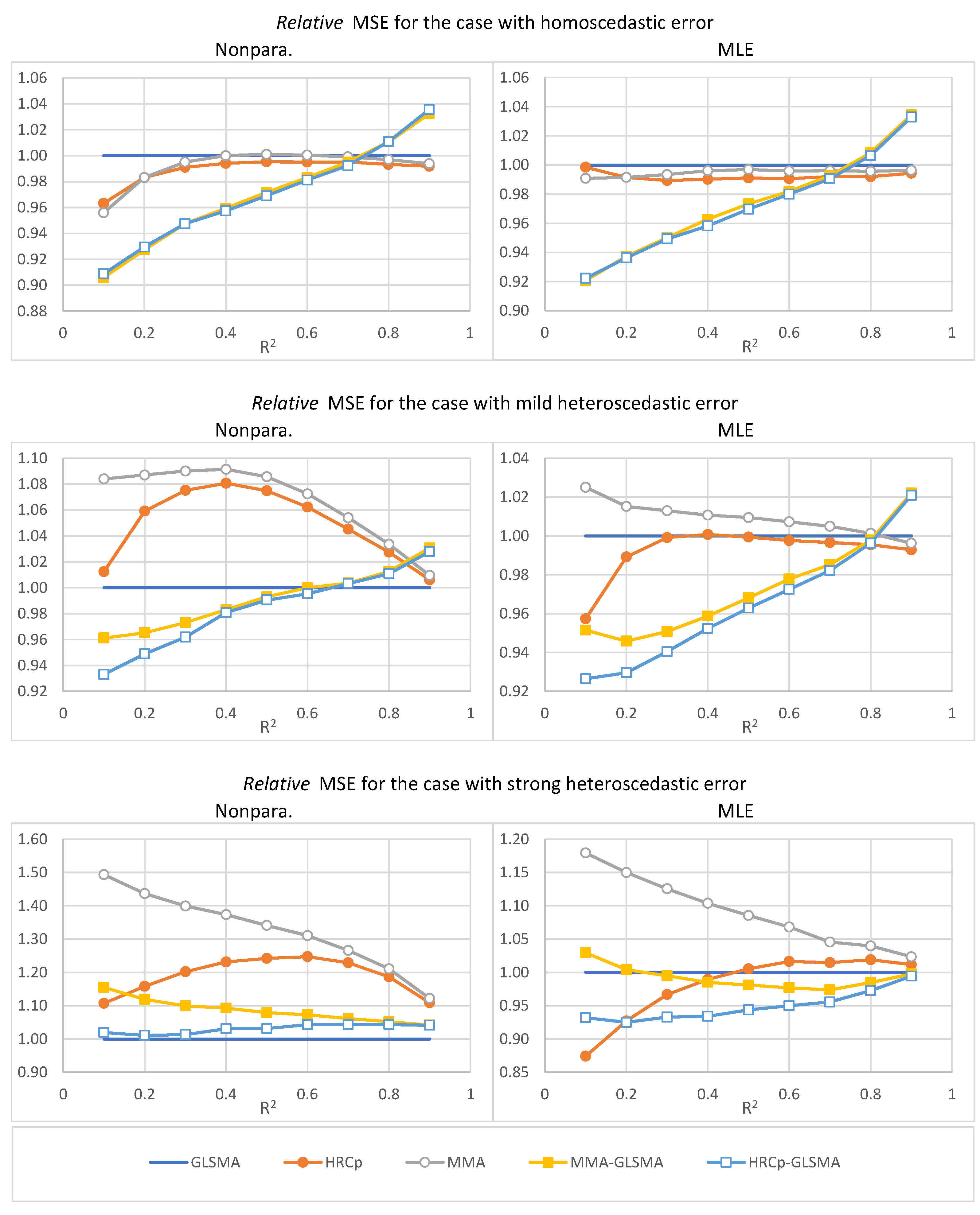
The number of replications for all simulations was 1000. We evaluated the performance of each method by the sample mean squared error (MSE) $=1/1000{\sum }_{k=1}^{1000}{∥{\widehat{\mu }}_{\left(k\right)}-{\mu }_{\left(k\right)}∥}^2$, where ${\widehat{\mu }}_{\left(k\right)}$ and ${\mu }_{\left(k\right)}$ are the realized vector of the estimated value $\widehat{\mu }$ and true value $\mu$ in the $k^{\mathrm{th}}$ replication, respectively. The simulation results are shown in

Table 1. Sample mean squared error (MSE) for the case with homoscedastic error.

	${\mathit{R}}^2$	GLSMA	HRCp	MMA	MMA-GLSMA	HRCp-GLSMA
	$0.1$	6.80	6.55	6.50	6.16	6.18
	$0.2$	9.50	9.34	9.34	8.81	8.83
	$0.3$	12.20	12.09	12.14	11.56	11.56
	$0.4$	15.25	15.16	15.25	14.63	14.60
Nonpara.	$0.5$	19.06	18.97	19.08	18.52	18.47
	$0.6$	24.33	24.21	24.34	23.92	23.87
	$0.7$	32.64	32.48	32.61	32.48	32.39
	$0.8$	48.66	48.33	48.51	49.18	49.19
	$0.9$	95.66	94.88	95.07	98.76	99.08
	$0.1$	6.56	6.55	6.50	6.04	6.05
	$0.2$	9.42	9.34	9.34	8.83	8.82
	$0.3$	12.22	12.09	12.14	11.61	11.60
	$0.4$	15.31	15.16	15.25	14.74	14.67
MLE	$0.5$	19.14	18.97	19.08	18.63	18.56
	$0.6$	24.44	24.21	24.34	24.00	23.95
	$0.7$	32.74	32.48	32.61	32.50	32.43
	$0.8$	48.72	48.33	48.51	49.13	49.04
	$0.9$	95.42	94.88	95.07	98.70	98.56

,

Table 2. Sample MSE for the case with mild heteroscedastic error.

	${\mathit{R}}^2$	GLSMA	HRCp	MMA	MMA-GLSMA	HRCp-GLSMA
	$0.1$	6.43	6.51	6.97	6.18	6.00
	$0.2$	8.62	9.13	9.37	8.32	8.18
	$0.3$	10.77	11.58	11.74	10.48	10.36
	$0.4$	13.02	14.07	14.21	12.80	12.77
Nonpara.	$0.5$	15.76	16.94	17.11	15.65	15.61
	$0.6$	19.45	20.66	20.86	19.45	19.36
	$0.7$	25.20	26.34	26.56	25.29	25.28
	$0.8$	36.05	37.04	37.26	36.50	36.44
	$0.9$	67.46	67.87	68.10	69.53	69.34
	$0.1$	6.80	6.51	6.97	6.47	6.30
	$0.2$	9.23	9.13	9.37	8.73	8.58
	$0.3$	11.59	11.58	11.74	11.02	10.90
	$0.4$	14.06	14.07	14.21	13.48	13.39
MLE	$0.5$	16.95	16.94	17.11	16.41	16.32
	$0.6$	20.71	20.66	20.86	20.25	20.14
	$0.7$	26.43	26.34	26.56	26.04	25.96
	$0.8$	37.21	37.04	37.26	37.13	37.07
	$0.9$	68.36	67.87	68.10	69.86	69.79

and

Table 3. Sample MSE for the case with strong heteroscedastic error.

	${\mathit{R}}^2$	GLSMA	HRCp	MMA	MMA-GLSMA	HRCp-GLSMA
	$0.1$	13.44	14.88	20.07	15.52	13.70
	$0.2$	16.13	18.68	23.17	18.05	16.30
	$0.3$	18.92	22.74	26.47	20.80	19.17
	$0.4$	22.02	27.11	30.24	24.06	22.69
Nonpara.	$0.5$	25.91	32.18	34.74	27.96	26.73
	$0.6$	30.89	38.52	40.48	33.13	32.21
	$0.7$	38.28	47.03	48.46	40.62	39.94
	$0.8$	51.15	60.68	61.92	53.80	53.37
	$0.9$	85.65	94.97	96.06	89.21	89.15
	$0.1$	17.02	14.88	20.07	17.52	15.86
	$0.2$	20.15	18.68	23.17	20.23	18.64
	$0.3$	23.52	22.74	26.47	23.40	21.94
	$0.4$	27.40	27.11	30.24	26.99	25.59
MLE	$0.5$	32.01	32.18	34.74	31.40	30.21
	$0.6$	37.90	38.52	40.48	37.02	36.00
	$0.7$	46.35	47.03	48.46	45.13	44.29
	$0.8$	59.56	60.68	61.92	58.65	57.93
	$0.9$	93.86	94.97	96.06	93.65	93.33

. Figure 1 presents the same information relative to the MSE of the GLSMA method.

The results in Table 1 and Table 2 show that our combination methods, MMA-GLSMA and HRCp- GLSMA, performed better than the alternatives (GLSMA, HRCp and MMA) when the error term was homoscedastic or had mild heteroscedasticity for $R^2\le 0.7$. When $R^2\ge 0.8$, the performance of our methods was slightly worse than that of the alternative methods. For the homoscedastic case, the three alternative methods performed similarly. On the other hand, in the case of mild heteroscedasticity, GLSMA and $HR{C}_p$ performed better than MMA (which was expected, as MMA was designed for homoscedastic models).

Table 3 demonstrates that, when the heteroscedasticity of the error term was considerably strong, our combination method HRCp-GLSMA worked much better than the others when the MLE-based estimation of ${\sigma }_i$ was used. However, MMA-GLSMA and HRCp-GLSMA became worse than GLSMA when ${\sigma }_i$ was estimated using the nonparametric method.

Moreover, for most cases, GLSMA with the nonparametric estimator of ${\sigma }_i$ outperformed GLSMA with the MLE-based estimator of ${\sigma }_i$. This can be explained by a characteristic of the k-NN method that we adopted. In the k-NN estimation, a large weight was placed on the $i^{\mathrm{th}}$ squared residual to estimate ${\sigma }_i^2$; therefore, even though ${\sigma }_i^2$ was misspecified, the estimate could catch the heteroscedasticity of the error term to some extent.

The aforementioned simulation results gave us the following indications for practical analysis. If we know that the heteroscedasticity of the data is considerably strong or the population $R^2$ is large, we should use the nonparametric GLSMA. Otherwise, it is preferable to choose an MMA-GLSMA or HRCp-GLSMA combination.

Table 4. Averages of the OLS (${\overline{W}}_1$) and GLS (${\overline{W}}_2$) parts of the weight vector for HRCp-GLSMA.

${\mathit{R}}^2$	0.1	0.2	0.3	0.4	0.5	0.6	0.7	0.8	0.9
Homoscedastic Cases
Nonp.OLS (${\overline{W}}_1$)	0.50	0.50	0.50	0.50	0.49	0.49	0.49	0.49	0.49
Nonp. GLS (${\overline{W}}_2$)	0.50	0.50	0.50	0.50	0.51	0.51	0.51	0.51	0.51
MLE OLS (${\overline{W}}_1$)	0.50	0.50	0.50	0.50	0.50	0.50	0.50	0.50	0.50
MLE GLS (${\overline{W}}_2$)	0.50	0.50	0.50	0.50	0.50	0.50	0.50	0.50	0.50
Mild Heteroscedastic Cases
Nonp. OLS (${\overline{W}}_1$)	0.49	0.49	0.49	0.49	0.49	0.49	0.49	0.49	0.49
Nonp. GLS (${\overline{W}}_2$)	0.51	0.51	0.51	0.51	0.51	0.51	0.51	0.51	0.51
MLE OLS (${\overline{W}}_1$)	0.49	0.49	0.49	0.49	0.49	0.49	0.50	0.50	0.50
MLE GLS (${\overline{W}}_2$)	0.51	0.51	0.51	0.51	0.51	0.51	0.50	0.50	0.50
Strong Heteroscedastic Cases
Nonp. OLS (${\overline{W}}_1$)	0.48	0.48	0.48	0.48	0.48	0.48	0.48	0.48	0.48
Nonp. GLS (${\overline{W}}_2$)	0.52	0.52	0.52	0.52	0.52	0.52	0.52	0.52	0.52
MLE OLS (${\overline{W}}_1$)	0.49	0.49	0.49	0.49	0.49	0.49	0.49	0.49	0.49
MLE GLS (${\overline{W}}_2$)	0.51	0.51	0.51	0.51	0.51	0.51	0.51	0.51	0.51

and

Table 5. Averages of the OLS (${\overline{W}}_1$) and GLS (${\overline{W}}_2$) parts of the weight vector for MMA-GLSMA.

${\mathit{R}}^2$	0.1	0.2	0.3	0.4	0.5	0.6	0.7	0.8	0.9
Homoscedastic Cases
Nonp. OLS (${\overline{W}}_1$)	0.50	0.49	0.49	0.49	0.49	0.49	0.49	0.49	0.49
Nonp. GLS (${\overline{W}}_2$)	0.50	0.51	0.51	0.51	0.51	0.51	0.51	0.51	0.51
MLE OLS (${\overline{W}}_1$)	0.50	0.50	0.50	0.50	0.50	0.50	0.50	0.50	0.50
MLE GLS (${\overline{W}}_2$)	0.50	0.50	0.50	0.50	0.50	0.50	0.50	0.50	0.50
Mild Heteroscedastic Cases
Nonp. OLS (${\overline{W}}_1$)	0.50	0.49	0.49	0.49	0.49	0.49	0.49	0.49	0.49
Nonp. GLS (${\overline{W}}_2$)	0.50	0.51	0.51	0.51	0.51	0.51	0.51	0.51	0.51
MLE OLS (${\overline{W}}_1$)	0.50	0.50	0.50	0.50	0.50	0.50	0.50	0.50	0.50
MLE GLS (${\overline{W}}_2$)	0.50	0.50	0.50	0.50	0.50	0.50	0.50	0.50	0.50
Strong Heteroscedastic Cases
Nonp. OLS (${\overline{W}}_1$)	0.50	0.50	0.49	0.49	0.49	0.49	0.49	0.49	0.49
Nonp. GLS (${\overline{W}}_2$)	0.50	0.50	0.51	0.51	0.51	0.51	0.51	0.51	0.51
MLE OLS (${\overline{W}}_1$)	0.50	0.50	0.50	0.50	0.50	0.50	0.50	0.50	0.50
MLE GLS (${\overline{W}}_2$)	0.50	0.50	0.50	0.50	0.50	0.50	0.50	0.50	0.50

give the averages of the estimated weights corresponding to the OLS and GLS parts for HRCp-GLSMA and MMA-GLSMA. Table 4 shows that for HRCp-GLSMA, when the heteroscedasticity became stronger, the average weights corresponding to the GLS part increased and the average weights corresponding to the OLS estimates decreased. Table 5 does not show a similar trend for MMA-GLSMA. This might be an explanation for why the performance of MMA-GLSMA was worse than that of HRCp-GLSMA.

5. Conclusions

In this paper, we proposed a combination method of OLS and GLS estimators. The proposed method reduced the risk of misspecification between homoscedastic and heteroscedastic models. The optimality of the criteria for choosing a weight vector was proven under some regularity conditions. We performed simulation experiments to investigate the finite sample property of our combination method. The results of the simulations demonstrate that our method was adaptive for homoscedasticity and heteroscedasticity. As mentioned previously, the proposed method was novel in that it combined estimators from two different estimation methods. Combining the different estimation methods can also combine the advantages of each. This idea could be useful and should be extended to the combination of other estimation methods.

References

- Danilov, Dmitry, and Jan R. Magnus. 2004. On The Harm That Ignoring Pretesting Can Cause. Journal of Econometrics 122: 27–46. [Google Scholar] [CrossRef]
- Hansen, Bruce E. 2007. Least Squares Model Averaging. Econometrica 75: 1175–89. [Google Scholar] [CrossRef]
- Hansen, Bruce E., and Jeffrey S. Racine. 2012. Jackknife Model Averaging. Journal of Econometrics 167: 38–46. [Google Scholar] [CrossRef]
- Li, Ker-Chau. 1987. Asymptotic Optimality for Cp, CL, Cross-Validation and Generalized Cross-Validation: Discrete Index Set. Annals of Statistics 15: 958–75. [Google Scholar] [CrossRef]
- Liu, Qingfeng, and Ryo Okui. 2013. Heteroscedasticity-Robust Cp Model Averaging. Econometrics Journal 16: 463–72. [Google Scholar] [CrossRef]
- Liu, Qingfeng, Ryo Okui, and Arihiro Yoshimura. 2016. Generalized Least Squares Model Averaging. Econometric Reviews 35: 1692–752. [Google Scholar] [CrossRef]
- Makridakis, Spyros, Evangelos Spiliotis, and Vassilios Assimakopoulos. 2018. The M4 Competition: Results, Findings, Conclusion and Way Forward. International Journal of Forecasting 34: 802–8. [Google Scholar] [CrossRef]
- Wan, Alan TK, Xinyu Zhang, and Guohua Zou. 2010. Least Squares Model Averaging by Mallows Criterion. Journal of Econometrics 156: 277–83. [Google Scholar] [CrossRef]
- Xie, Tian. 2017. Heteroscedasticity-Robust Model Screening: A Useful Toolkit for Model Averaging in Big Data Analytics. Economics Letters 151: 119–22. [Google Scholar] [CrossRef]
- Yuan, Zheng, and Yuhong Yang. 2005. Combining Linear Regression Models: When and How? Journal of the American Statistical Association 100: 1202–14. [Google Scholar] [CrossRef]
- Zhang, Xinyu, Alan TK Wan, and Guohua Zou. 2013. Model Averaging by Jackknife Criterion in Models with Dependent Data. Journal of Econometrics 174: 82–94. [Google Scholar] [CrossRef]
- Zhang, Xinyu, Guohua Zou, and Raymond J. Carroll. 2015. Model Averaging Based on Kullback-Leibler Distance. Statistica Sinica 25: 1583–98. [Google Scholar] [CrossRef] [PubMed]
- Zhao, Shangwei, Aman Ullah, and Xinyu Zhang. 2018. A Class of Model Averaging Estimators. Economics Letters 162: 101–6. [Google Scholar] [CrossRef]
Figure 1.
Performance of the methods relative to generalized least-squares model averaging (GLSMA): Heteroscedasticity-robust Cp (HRCp), Mallows model averaging (MMA), MMA-GLSMA and HRCp-GLSMA.