On the Forecast Combination Puzzle

1
Department of Applied Economics and Statistics, University of Delaware, Newark, DE 19716, USA
2
School of Statistics, University of Minnesota, Minneapolis, MN 55455, USA
*
Author to whom correspondence should be addressed.
Econometrics 2019, 7(3), 39; https://0-doi-org.brum.beds.ac.uk/10.3390/econometrics7030039
Submission received: 15 June 2019
/
Revised: 29 August 2019
/
Accepted: 6 September 2019
/
Published: 10 September 2019
(This article belongs to the Special Issue Bayesian and Frequentist Model Averaging)
Abstract
:It is often reported in the forecast combination literature that a simple average of candidate forecasts is more robust than sophisticated combining methods. This phenomenon is usually referred to as the “forecast combination puzzle”. Motivated by this puzzle, we explore its possible explanations, including high variance in estimating the target optimal weights (estimation error), invalid weighting formulas, and model/candidate screening before combination. We show that the existing understanding of the puzzle should be complemented by the distinction of different forecast combination scenarios known as combining for adaptation and combining for improvement. Applying combining methods without considering the underlying scenario can itself cause the puzzle. Based on our new understandings, both simulations and real data evaluations are conducted to illustrate the causes of the puzzle. We further propose a multi-level AFTER strategy that can integrate the strengths of different combining methods and adapt intelligently to the underlying scenario. In particular, by treating the simple average as a candidate forecast, the proposed strategy is shown to reduce the heavy cost of estimation error and, to a large extent, mitigate the puzzle.
1. Introduction
Since the seminal work of Bates and Granger (1969), both empirical and theoretical investigations support that when multiple candidate forecasts for a target variable are available to an analyst, forecast combination often provides more accurate forecasting performance in terms of mean squared forecast error (MSFE) than using a single candidate forecast. The benefits of forecast combination are attributable to the fact that individual forecasts often use different sets of information, are subject to model bias from different, but unknown model misspecifications, and/or are varyingly affected by structural breaks. The review of Timmermann (2006) provided a comprehensive account of various forecast combination methods. Usually, the attention is on an optimal weight as a theoretically best choice within a scope of consideration (e.g., the best linear or convex combination that minimizes forecast risk). Correspondingly, one popular combining strategy is the pursuit of the target optimal weight through a sensible minimization of MSFE. For example, Bates and Granger (1969) proposed to estimate the optimal weight using the error variance-covariance structure of the individual forecasts. Granger and Ramanathan (1984) approximated the optimal weight under a linear regression framework.
With rapid advances in data-driven technology, forecast combination and model averaging methods have become increasingly popular and fruitful research areas. In particular, combining methods are usually approached under either frequentist or Bayesian frameworks. From the frequentist perspective, combining methods are developed for various specific statistical prediction and forecasting tasks (often based on least-squares criteria) such as linear regression, factor models, generalized linear models, treatment effects estimation, and spatial modeling, among many others (e.g., Yang 2004, Wan et al. 2010, Ando and Li 2014; Cheng et al. 2015; Cheng and Hansen 2015; Zhang et al. 2016; Zhu et al. 2018; Zhang and Yu 2018, and the references therein). Bayesian-based averaging techniques are also powerful and well-developed tools in many important forecasting scenarios (e.g., Hoeting et al. 1999, Steel 2011; Garcia-Donato and Martinez-Beneito 2013; Steel 2014; Forte et al. 2018, and the references therein). Furthermore, methods that take mixed flavor on frequentist and Bayesian techniques are known to be promising approaches to model averaging and combining (e.g., Magnus and De Luca 2016; Magnus et al. 2016; De Luca et al. 2018 and the references therein). Methods inspired by screening (e.g., Fan and Lv 2008; Fan and Song 2010), shrinkage (e.g., Tibshirani 1996; Zou 2006), sequential stepwise (e.g., Zhang 2011; Ing and Lai 2011; Qian et al. 2019), and/or greedy boosting (e.g., Friedman et al. 2000; Friedman 2001; Yang et al. 2018) techniques are also developed for combining models under high-dimensional scenarios (e.g., J. Chen et al. 2018, Lan et al. 2019, and the references therein).
Despite the popularity and sophistication of combining methods, empirical studies have repeatedly reported that the simple average (SA) is an effective and robust combination method that often outperforms more complicated methods (see Winkler and Makridakis 1983, Clemen and Winkler 1986, and Diebold and Pauly 1990 for some early examples). In a review and annotated bibliography on early studies, Clemen (1989) raised the question, “What is the explanation for the robustness of the simple average of forecasts?”. Specifically, he proposed two questions of interest, “(1) Why does the simple average work so well, and (2) under what conditions do other specific methods work better?” The robustness of SA is also echoed in more recent literature. For example, Stock and Watson (2004) built autoregressive models with univariate predictors (macroeconomic variables) as candidate forecasts for the output growth of seven developed countries and found that SA, together with other methods of least data adaptivity, is among the top-performing forecast combination methods. Stock and Watson (2004) further coined the term “forecast combination puzzle” (FCP), which refers to “the repeated finding that simple combination forecasts outperform sophisticated adaptive combination methods in empirical applications”. In another recent example, Genre et al. (2013) used survey data from professional forecasters as the individual candidates to construct combined forecasts for three target variables. Despite some promising results of complicated methods, they further noted that the observed improvement over SA was rather vague when a period of financial crisis was included in the analysis. Past empirical evidence appears to support the mysterious existence of FCP, which was also summarized in Timmermann (2006) (Section 7.1).
Many attempts have been made to demystify FCP. One popular and arguably the most well-studied explanation for FCP is the estimation error of methods that target the optimal combination weights. Smith and Wallis (2009) rigorously studied the estimation error issue. Using the forecast error variance-covariance structure, they showed both theoretically and numerically that the estimator targeting the optimal weight can have large variance, and consequently, the estimated optimal weight can be very different from the true optimal weight, often even more so than the simple equal weight. Elliott (2011) studied the theoretical maximal performance gain of the optimal weight over SA by optimizing the error variance-covariance structure and pointed out that the gain is often small enough to be overshadowed by estimation error. Timmermann (2006) and Hsiao and Wan (2014) also illustrated conditions for the optimal weight to be close to the equal weight, so that the relative gain of the optimal weight over SA is small. Claeskens et al. (2016) considered the random weight and showed that when the weight variance is taken into account, SA can perform better than using the “optimal” weight. Under linear regression settings, Huang and Lee (2010) discussed the estimation error and the relative gain of the optimal weight. Interestingly, the recent development in the M4competition (Makridakis et al. 2018) and several other studies (e.g., L. Chen et al. 2018) showed evidence that SA can be sub-optimal compared to some forecast combining methods although SA remains to be a good benchmark; the important progress echos part of our paper’s conclusions, and the investigation on the classical FCP issues provides a relevant and useful platform for helping to understand in depth the large performance difference observed for combination methods.
Following the FCP literature, unless stated otherwise, all the “estimation errors” we will mention in this article are with respect to the estimation of the target optimal weight. We should not confuse these estimation errors with those for estimating parameters in statistical models (based on which forecasts are made). Although the understanding of the latter estimation errors is an important topic in its own right, it is not directly relevant to our discussion. Indeed, it is not uncommon to assume that an analyst is agnostic about and may have no control over how the candidate forecasts are generated. These candidate forecasts can be obtained from expert opinions or their underlying statistical models can be proprietary. Throughout this article, we are concerned about how to understand combinations of existing candidate forecasts rather than how to explain forecast errors of the individual candidate forecasts.
In addition to estimation error, nonstationarity and structural breaks in the data generating process (DGP) are believed to contribute to the unstable performance of the estimated “optimal” weight. For example, Hendry and Clements (2004) demonstrated that when candidate forecasting models are all misspecified and breaks occur in the information variables, forecast combination methods that target the optimal weight may not perform as well as SA. From the perspective of candidate forecasts, Lahiri et al. (2013) suggested that during periods of unstable relative performance, adjusting the weights agilely based on recent observations can sometimes hurt the aggregate forecast performance compared to maintaining the weights cautiously. Besides structural breaks, they attributed this phenomenon to forecast outliers, the effects of which can be mitigated by the robust methods proposed in Cheng and Yang (2015). Huang and Lee (2010) proposed that the candidate forecasts are often weak; that is, they have low predictive content on the target variable, making the optimal weight similar to the simple equal weight.
While the aforementioned points are valid and valuable, they do not seem to depict the complete picture of the puzzle. In this paper, we provide our perspectives on FCP to contribute to its settling. In our view, besides providing explanations of FCP, it is also important to point out the potential danger of recommending SA for broad and indiscriminate use. Here, we focus on the mean squared error (MSE). It should be pointed out that the main points are expected to stand for other losses as well (e.g., absolute error) and that some combination approaches (e.g., AFTER, Yang 2004; Zhang et al. 2013) can handle general loss functions.
The rest of this article is organized as follows. In Section 2, we list some aspects of FCP that have not been much addressed, but are important for understanding the puzzle in our view. The forecast combination problem we consider is formally introduced in Section 3. Our understandings of FCP are elaborated in Section 4, Section 5, Section 6, Section 7 and Section 8, which include the existence of two distinct scenarios (combining for adaptation vs. combining for improvement), improperly derived weighting formulas, and the prevalent use of model screening. We argue that SA is not as robust as is often believed. In particular, Section 5 proposes a multi-level AFTER approach in an attempt to mitigate FCP. The performance of this approach is also evaluated in Section 9 using data from the U.S. Survey of Professional Forecasters (SPF). A brief conclusion is given in Section 10. Some theoretical results are collected in the Appendix.
2. Additional Aspects of FCP
The previous work nicely pointed out that estimation error is an important source of FCP and characterized the impact of the estimation error in certain settings. Indeed, in general, when the forecast combination weighting formula is valid in the sense that an optimal weight can be correctly estimated by minimizing MSFE, an insufficiently small sample size may not support reliable estimation of the weight, resulting in inflated variance of the combined forecast. The explanation with structural breaks also makes sense for certain situations. Furthermore, in our view, there are several additional aspects that may need to be considered for understanding FCP.
- A key factor missing in addressing the FCP is the true nature of the improvability of the candidate forecasts. While we all strive for better forecast performance than the candidates, that may not be feasible (at least for the methods considered). Thus, we have two scenarios (Yang 2004): (i) One of the candidates is pretty much the best we can hope for (within the considerations of course), and consequently, any attempt to beat it becomes futile. We refer to this scenario as “combining for adaptation” (CFA), because the proper goal of a forecast combination method under this scenario should be targeting the performance of the best individual candidate forecast, which is unknown. (ii) The other scenario is that a significant accuracy gain over all the individual candidates can be realized by combining the forecasts. We refer to this scenario as “combining for improvement” (CFI), because the proper goal of a forecast combination method under this scenario should be targeting the performance of the best combination of the candidate forecasts to overcome the defects of the candidates. In practical applications, both scenarios could be possible. Without factoring in this aspect, comparison of different combination methods may become somewhat misleading. In our view, bringing this lurking aspect into the analysis is beneficial to understand forecast combinations. With the above forecast combination scenarios spelled out, a natural question follows: can we design a combination method to bridge the two camps of methods proposed for the two scenarios? That is, in practical applications, without necessarily knowing the underlying forecast scenario, can we have a combination strategy adaptive to both scenarios?
- The methods being examined in the literature on FCP are mostly specific choices (e.g., least squares estimation). Can we do better with other methods (that may or may not have been invented yet) to mitigate relatively heavy estimation price? Furthermore, it is often assumed that the forecasts are unbiased and the forecast errors are stationary, which may not be proper for many applications. What happens when these assumptions do not hold?
- It has been stated in the literature that the simple methods (e.g., SA) are robust based on empirical studies. This may not be necessarily true in the usual statistical sense (rigorously or loosely). In many published empirical results, the candidate forecasts were carefully selected/built and thus well-behaved. Therefore, the finding in favor of the robustness of SA may be proper only for such situations in which the data analyst has extensive expertise on the forecasting problem and has done quite a bit of work on screening out poor/un-useful candidates; when allowing for the possibility of poor/redundant candidates for wider applications, the FCP may not be applicable anymore. It should be added that in various situations, the screening of forecasts are far from being an easy task, and the complexity may well be at the same level as model selection/averaging. Therefore, the view that we can do a good job in screening the candidate forecasts and then simply recruit SA can be overly optimistic. With the above, it is important to examine the robustness of SA in a broader context.
As is described in the first aspect, there are two distinct scenarios: CFA and CFI. The CFA scenario can happen if one of the candidate forecasts is based on a model sophisticated enough to capture the true DGP (yet still relatively simple to permit accurate estimation of the parameters) and/or the other candidate forecasts only add redundant information. The CFI scenario can often happen when different candidate forecasts use different information, and/or their underlying models have misspecifications in different ways. The scenarios of CFA vs. CFI are also echoed by the discussion of forecast selection vs. combination to a certain degree (e.g., Kourentzes et al. 2019 and the references therein), although this paper is solely focused on understanding forecast combination methods.
There are various existing combining methods designed for the two scenarios. The methods for the CFI scenario typically seek to estimate the optimal weight, and their examples include classical variance-covariance-based optimization (Bates and Granger 1969), linear regression (Granger and Ramanathan 1984), and more recent frequentist (often based on least-squares criteria) methods discussed in the Introduction. On the other hand, the combining methods for the CFA scenario should ideally perform similarly to the best individual candidate forecast. The typical methods suitable for the CFA scenario include AIC model averaging (Buckland et al. 1997) and Bayesian model averaging, often in parametric settings. The method of AFTER (Yang 2004) and various exponential-weighting-based averaging procedures (e.g., Yang 2001; Rolling et al. 2018) may be used in both parametric and non-parametric settings.
Clearly, these two camps of methods (CFI vs. CFA) are designed with very different purposes. The former is in some sense more “aggressive” that the methods are designed to target the optimal weight in order to improve forecast accuracy over all candidate forecasts. The latter is relatively “conservative” in the sense that the methods are only designed to match the performance of the best candidate. Intuitively, to achieve the more aggressive target, the former methods are expected to pay a somewhat higher estimation price, and applying them under a CFA scenario may lead to suboptimal results. On the other hand, it is not ideal either to apply the latter methods under a CFI scenario since such practice violates the original design purpose of these methods. As one contribution, we offer the distinction between the two scenarios that can contribute to understanding the FCP. We will see in Section 4 that failing to bring in the underlying scenarios and specific types of data when choosing the combining methods may result in incorrectly applying a combining method not designed for the underlying scenario and consequently delivering forecasting results worse than other simple alternatives (including SA). In addition, as will be discussed later, we offer a practically adaptive solution called multi-level AFTER (mAFTER) to help bridge the theory and practice in face of uncertain forecast scenarios.
Related to the first two aspects regarding whether we can mitigate the estimation price, we cannot fully address them without a proper framework, because for any sensible method, one can always find a situation to favor it over its competitors. The framework we consider with theoretical support is through a minimax view: If one has a specific class of combination of the forecasts in mind and wants to target the best combination in this class, then without any restriction/assumption on the unbiasedness of the candidate forecasts and the stationarity of the forecast errors, the minimax view seeks an understanding of the minimum price we have to pay no matter what method (existing or not) is used for combining. It turns out that the framework from the minimax view is closely related to the forecast combination scenarios discussed in the first aspect.
Indeed, Yang (2004) showed that from a minimax perspective, because of the relatively aggressive target set for the CFI scenario, we have to pay a heavier cost than the target set for the CFA scenario. Specifically, if we let K denote the number of forecasts and T denote the forecasting horizon, when the target is to find the optimal weight to minimize the forecast risk over a set of weights satisfying a convex constraint (which is appropriate under the CFI scenario), the estimation cost is for relatively large T () and for relatively small T () (note that the bounds can be slightly improved to be exactly minimax optimal; see, e.g., Wang et al. (2014) in a simpler setting). In contrast, if the target is to match the performance of the best individual forecast (which is appropriate under the CFA scenario), the estimation cost is reduced to , which tends to be smaller than that of the CFI scenario.
Due to the relatively heavy cost under the CFI scenario, it may not be always ideal to pursue the goal of the optimal weight. Indeed, even if the optimal weight gives better performance than the best individual candidate, the improvement may not be enough to offset the additional estimation cost (i.e., increased variance) as identified in Yang (2004) and Wang et al. (2014). As another contribution, we show in Section 6 that an appropriately-constructed forecast combination strategy (mAFTER) can perform in an intelligent way according to the underlying CFI or CFA scenario. If CFI is the correct scenario, the proposed strategy can behave both aggressively and conservatively so that it performs similarly to SA when SA is much better than, e.g., the linear regression method, and similarly to the latter when SA is worse.
Besides the estimation error and necessary distinction of the underlying scenarios discussed in the first two aspects, the following three straightforward reasons can also contribute to FCP. First, the weighting derivation formula used by complicated methods may not be suitable for the situation. For example, under structural breaks, old historical data no longer hold support for a valid optimal weighting scheme, and the known justification of well-established combining methods fails as a result (Hendry and Clements 2004). In Section 7, our Monte Carlo examples also show that SA may dominate the complicated methods when breaks occur in DGP dynamics. Second, it is common practice that the candidate forecasts are already screened in some ways so that they are more or less on an equal footing. For example, Stock and Watson (1998) and Stock and Watson (2004) applied various model selection methods such as AIC and BIC to identify promising linear or nonlinear candidate forecast models. Bordignon et al. (2013) selected models of different types (ARMAX, time-varying coefficients, etc.) and suggested that SA works well when combining a small number of well-performing forecasts. In studies using survey data of professional forecasters, it is also expected that each professional forecaster performs some model screening before satisfactorily settling down with his/her own forecast. In these cases, there may not be particularly poor candidate forecasts, and the candidates (at least the top ones) tend to contribute more or less equally to the optimal combination, making SA a competitive method. In Section 8, we use Monte Carlo examples to show that screening can be a source of FCP. Lastly, the puzzle can also be a result of publication bias; people expect sophisticated methods to work better than simple ones and tend to emphasize their surprising results when the converse is actually observed.
Furthermore, we partially address the issues raised in the third aspect and provide some auxiliary information on the behavior of SA in Section 6, Section 7 and Section 8. In particular, SA’s performance may change significantly or even substantially when an optimal, poor, or redundant forecast is added or the degree of the screening of the candidate forecasts is done differently, among others.
3. Problem Setup
Suppose that an analyst is interested in forecasting a real-valued time series . Given each time point , let be the (possibly multivariate) information variable vector revealed prior to the observation of . The may not be accessible to the analyst. Conditional on and , is subsequently generated from some unknown distribution with conditional mean and conditional variance . Then, can be represented as , where is the random noise with conditional mean and conditional variance being zero and , respectively.
Assume that prior to the observation of , the analyst has access to K real-valued candidate forecasts (). These forecasts may be constructed with different model structures, and/or with different components of the information variables, but the details regarding how each original forecast is created may not be available in practice and are not assumed to be known. The analyst’s objective in (linear) forecast combination is to construct a weight vector , based on the available information prior to the observation of , to find a point forecast of by forecast combination . The weight vector may be different at different time points. At time , the optimal weight minimizes the forecast risk of the combined forecast with in a given set (e.g., the set of all convex weight vectors, i.e., ; or the set of all real vectors, i.e., ). Alternatively, the optimal weights can also be defined conditionally by minimizing , where consists of all variables available for error prediction at time (Gibbs and Vasnev 2017).
To gauge the performance of a procedure that produces forecasts , given time horizon T, we consider the average forecast risk:
in our analysis and simulation studies. For real data evaluation, since the risk cannot be computed, we used the mean squared forecast error (MSFE) as a substitute:
According to the FCP, simple methods with little or no time variation in weight (e.g., equal weighting) often outperform complicated methods with much time variation in terms of and .
Since AFTER (Yang 2004) is one of the typical methods designed for the CFA scenario and plays an important role in our following discussion, we briefly describe the AFTER weight assignment procedure in the next subsection.
AFTER Method
At each time point (prior to the observation of ), AFTER updates the weight for the candidate forecasts based on their previous forecast performance and assigns to the forecast () the weight:
where is a pre-specified loss function, is a tuning parameter, and is an estimate of the conditional variance from the candidate forecast prior to the observation of . More explicitly, we can write (1) as an efficient weight updating scheme:
In practice, we can let be the sample variance of the previous forecast errors of the candidate forecast and set the tuning parameter to be one. Throughout this paper, we let be the quadratic loss . Under some mild regularity conditions, Theorem 5 in Yang (2004) shows that, in terms of the average forecast risk, AFTER can automatically match the performance of the best individual candidate forecast, with a relatively small price of for some positive constant .
4. CFA versus CFI: A Hidden Source of FCP
In this section, we study the performance of forecast combination methods under the two distinct scenarios discussed in Section 2. Not recognizing these scenarios can itself result in FCP. We used two simple, but illustrative Monte Carlo examples under regression settings similar to those of Huang and Lee (2010) to demonstrate the CFA and CFI scenarios.
- Case 1.
- Suppose () is generated by the linear model:where ’s are and ’s are independent of ’s and are . Consider the two candidate forecasts generated by:where and are both obtained from ordinary least squares (OLS) estimation using historical data.
Given that Forecast 1 essentially represents the true model, its combining with Forecast 2 cannot improve the performance of the best individual forecast asymptotically, thus giving an example of the CFA scenario. Let be a fixed start point of the evaluation period, and let T be the end point. Given the evaluation period from to T, let , , and be the average forecast risks of Forecast 1, Forecast 2, and the combined forecast, respectively. If we let be the average forecast risk at time T for SA, we expect that . Indeed, Proposition A1 in the Appendix A shows:
and asymptotically, the optimal combination assigns all the weight to Forecast 1. Under a CFA scenario such as this case, since the best candidate is unknown and often difficult to identify, the natural goal of forecast combination is to match the performance of the best candidate.
- Case 2.
- Suppose () is generated by the linear model:where the are following a bivariate normal distribution with mean and common variance . Let denote the correlation between and . The random error ’s are independent of ’s and are . Consider the two candidate forecasts generated by:where and are both obtained from OLS estimation with historical data.
Different from Case 1, Case 2 presents a scenario where each candidate forecast employs only part of the information set. It is expected, to some extent, that combining the two forecasts works like pooling different sources of important information, resulting in performance better than either of the candidate forecasts. By defining the average forecast risks the same way as in Case 1, we can see from Proposition A2 in the Appendix A that:
Clearly, when the two coefficients are not very different and the two information sets are not highly correlated, SA can significantly improve the forecast performance over the best candidate. This case gives one straightforward example of the CFI scenario, and it is appropriate to seek the more aggressive goal of finding the best linear combination of candidate forecasts.
Our view is that the discussion of the FCP should take into account the different combining scenarios. Next, we perform Monte Carlo studies on the two cases to provide an explanation. Combining methods suitable for the CFA scenario have been developed to target the performance of the best individual candidate. In our numerical studies, we chose the AFTER method (Yang 2004) as representative, and it is known that AFTER pays a smaller estimation price than methods that target the optimal linear or convex weighting. In contrast, combining methods for the CFI scenario usually attempt to estimate the optimal weight. For simplicity, we chose linear regression of the response on the candidate forecasts (LinReg) as the representative. The method of Bates and Granger (1969) without estimating correlation (BG) was used as an additional benchmark.
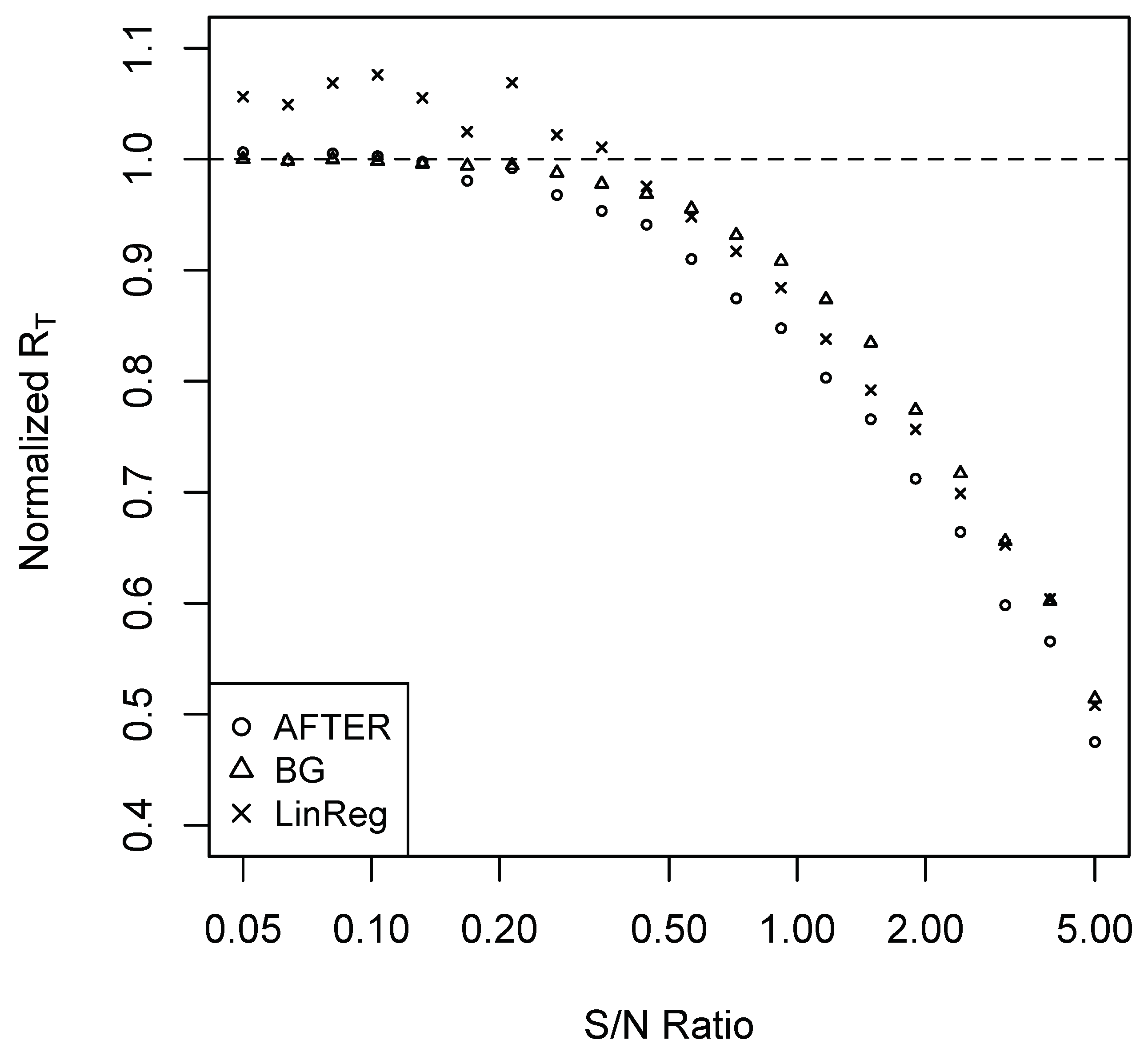
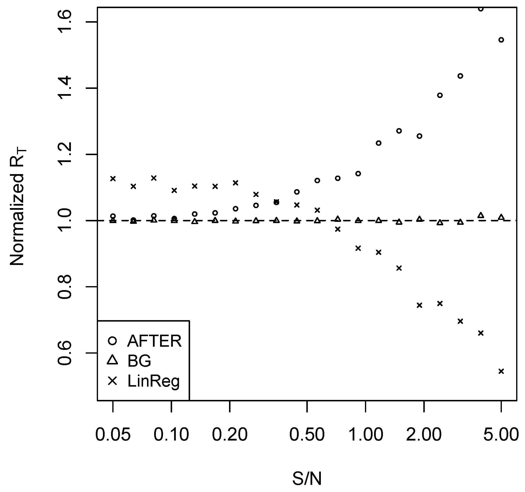
For Case 1, we performed simulations as follows. Set . Consider a sequence of 20 ’s such that the corresponding signal-to-noise (S/N) ratios are evenly spaced between 0.05 and five in the logarithmic scale. For each , we conduct the following simulation 100 times to estimate the average forecast risk. A sample of 100 observations is generated. The first 60 observations are used to build the candidate forecast models, which are subsequently used to generate forecasts for the remaining 40 observations. The methods of SA, BG, AFTER, and LinReg are applied to combine the candidate forecasts, and the last 20 observations are used for performance evaluation. The average forecast risk of each forecast combination method is divided by that of SA to obtain the normalized average forecast risk (denoted by normalized ). The results are summarized in Figure 1.
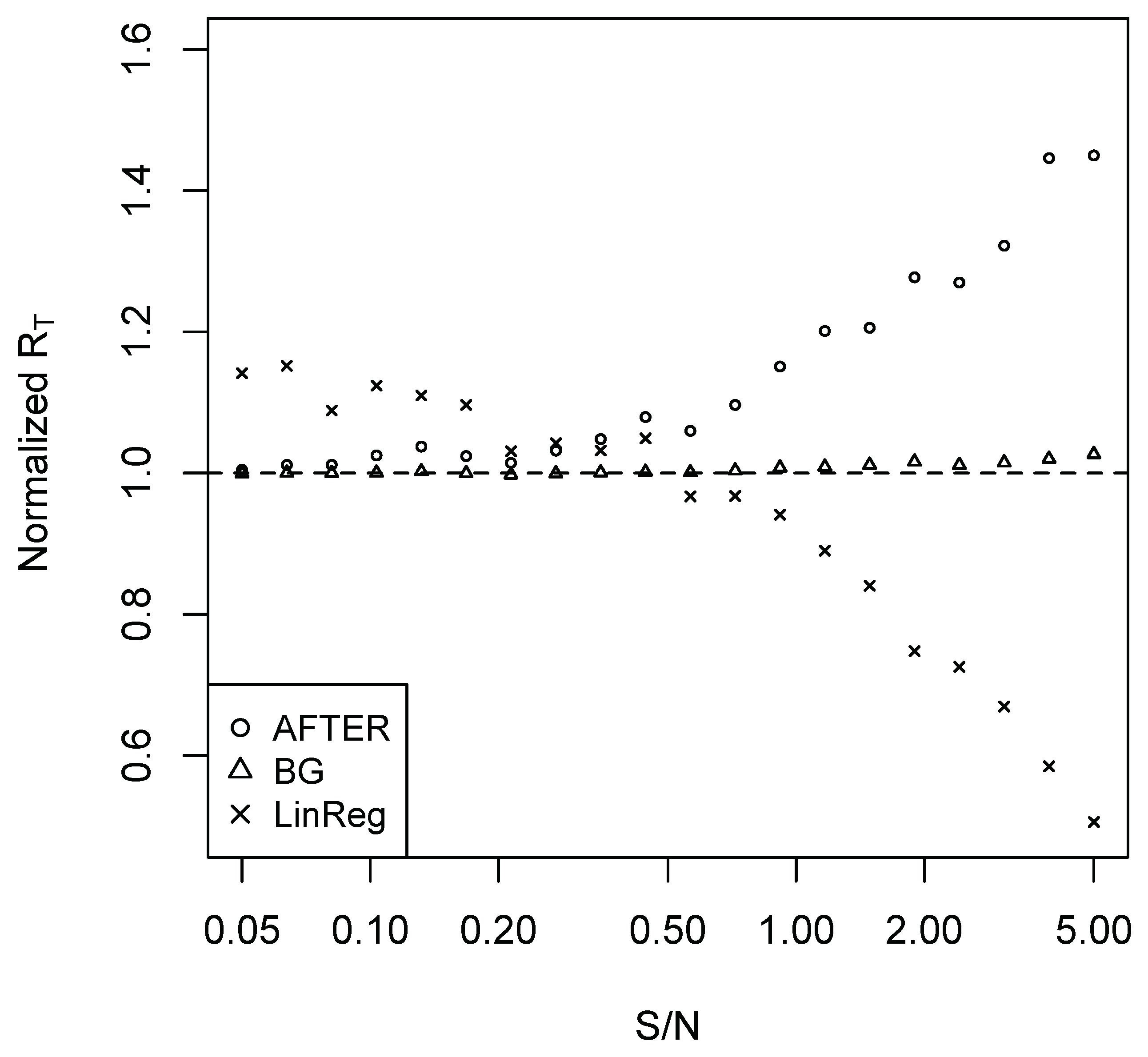
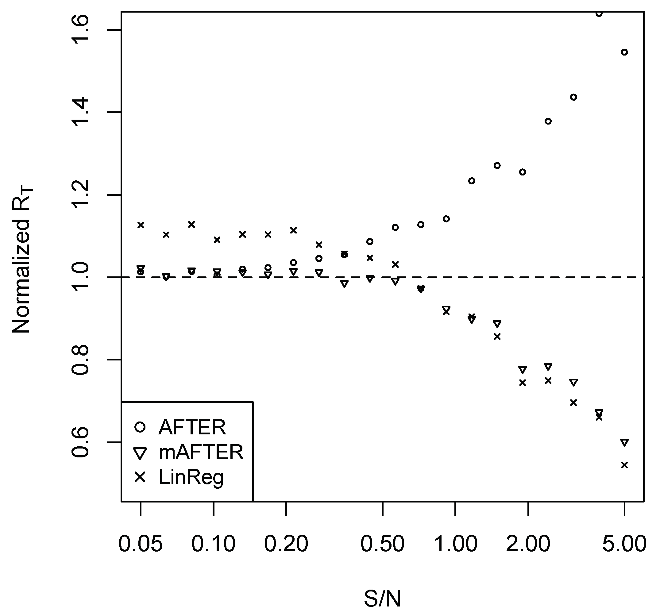
In Case 2, we set and for simplicity. The remaining simulation settings are the same as Case 1. The normalized average forecast risks (relative to SA) are summarized in Figure 2.
It is clear from Figure 1 that AFTER was the preferred method of choice under the CFA scenario presented in Case 1. LinReg, on the other hand, consistently underperformed compared to AFTER. Interestingly, when S/N was relatively low (less than 0.35), we observed the “puzzle” that LinReg performed worse than SA, which is due to the weight estimation error. If we correctly identify that it is the CFA scenario and apply a corresponding method like AFTER, the “puzzle” disappears: AFTER can perform better than (or very close to) SA.
In Case 2, if AFTER was applied under this CFI scenario, we observed the “puzzle” that SA outperformed AFTER. Once we understand the difference between the CFA and CFI scenarios, this “puzzle” is not surprising: while AFTER is designed to target the performance of the best individual forecast, (3) shows that SA can improve over the best individual forecast in Case 2. LinReg appeared to be the correct method of choice when the S/N ratio was relatively high. However, similar to what was observed in Case 1, LinReg suffered from weight estimation error when the S/N ratio was low, once again giving the “puzzle” that LinReg performed worse than SA.
Case 2 also shows the interesting observation that it was not always optimal to apply SA even when SA was the “optimal” weight in a restricted sense. Indeed, (A2) and (A3) in Proposition A2 imply that if we adopted the common restriction that the sum of all weights was one, SA was the asymptotic optimal weight. However, if we imposed no restriction on the weight range, the asymptotic optimal weight assigned a unit weight to each candidate forecast. This also explained the advantage of LinReg over SA in Case 2 when the S/N ratio was large.
In the simulation exposition, we also considered the information variables and () to have AR(1) model assumptions: for Case 1, assume satisfies:
where ’s are normally distributed random errors with mean zero and ’s are marginally normal with mean zero and variance ; for Case 2, assume ’s follow the same AR(1) settings as (4). We set and and repeated the same experiment as described before. The corresponding results on the normalized average forecast risk are summarized in Figure A1 and Figure A2 in the Appendix A, which show similar patterns as those of Figure 1 and Figure 2.
The observations above illustrate that different combining methods can have strikingly different performance depending on the underlying scenario. The FCP can appear when a combining method is not properly chosen according to the correct scenario. Without knowing the underlying scenario, comparing these methods may not provide a complete picture of FCP. We advocate the practice of trying to identify the underlying scenario (CFA or CFI) when considering forecast combination, which will be further explored in Rolling et al. (2019). It should be pointed out that when the relevant information is limited, it may not be feasible to identify confidently the forecast combination scenario. In such a case, a forced selection, similar to the comparison of model selection and model combining (averaging) described in Yuan and Yang (2005), would induce enlarged variability of the resulting forecast. An alternative reasonable solution could be an adaptive combination of forecasts as illustrated in the next section.
5. Multi-Level AFTER
With the understanding in Section 4, we see that when considering forecast combination methods, effort should be made to understand whether there is much room for improvement over the best candidate. When this is difficult to decide or impractical to implement due to handling a large number of quantities to be forecast in real time, we may turn to the question: Can we find an adaptive (or universal) combining strategy that performs well in both CFA and CFI scenarios? Note that here adaptive refers to adaptation to the forecast combination scenario (instead of adaptation to achieving the best individual performance). Another question follows: Under the CFI scenario, can the adaptive combining strategy still perform as well as SA when the price of estimation error is high? As we have seen in Case 2 of Section 4, using methods (e.g., LinReg) intended for the CFI scenario alone cannot successfully address the second question.
It turns out that the answers to these two questions are affirmative. The idea is related to a philosophical comment in Clemen et al. (1995, p. 134):
Any combination of forecasts yields a single forecast. As a result, a particular combination of a given set of forecasts can itself be thought of as a forecasting method that could compete...
The use of forecast (or procedure) combination is a theoretically powerful tool to achieve adaptive minimax optimality (e.g., Yang 2004; Wang et al. 2014). In the context of our discussion, combined forecasts such as SA, AFTER, and LinReg can all be considered as the candidate forecasts and may be used as individual candidates in a forecast combination scheme.
Accordingly, we designed a two-step combining strategy: first, we constructed three new candidate forecasts using SA, AFTER, and LinReg; second, we applied the AFTER algorithm on these new candidate forecasts to generate a combined forecast. We refer to this two-step algorithm as multi-level AFTER (mAFTER) because two layers of the AFTER algorithms are involved. The key lies in the AFTER algorithm in the second step, which allows mAFTER to target automatically the performance of the best individual candidate among SA, AFTER, and LinReg. Under the CFA scenario, mAFTER can perform as if we are using AFTER alone considering that AFTER is the proper method of choice. Under the CFI scenario, mAFTER can perform close to the better of SA and LinReg. Thus, when LinReg has relatively high estimation error, mAFTER will perform close to SA and thereby reduce the high cost.
Indeed, if we denote the forecasts generated from SA, LinReg, and mAFTER by , , and , respectively, we have Proposition 1 as follows.
Proposition 1.
Under the regularity conditions shown in the Appendix A, the average forecast risk of the mAFTER strategy satisfies:
where and are some positive constants not depending on the time horizon T.
Proposition 1 is a consequence of Theorem 5 in Yang (2004). It indicates that, in terms of the average forecast risk, mAFTER can match the performance of the best original individual forecast, the SA forecast, and the LinReg forecast (whichever is the best), with a relatively small price of order at most .
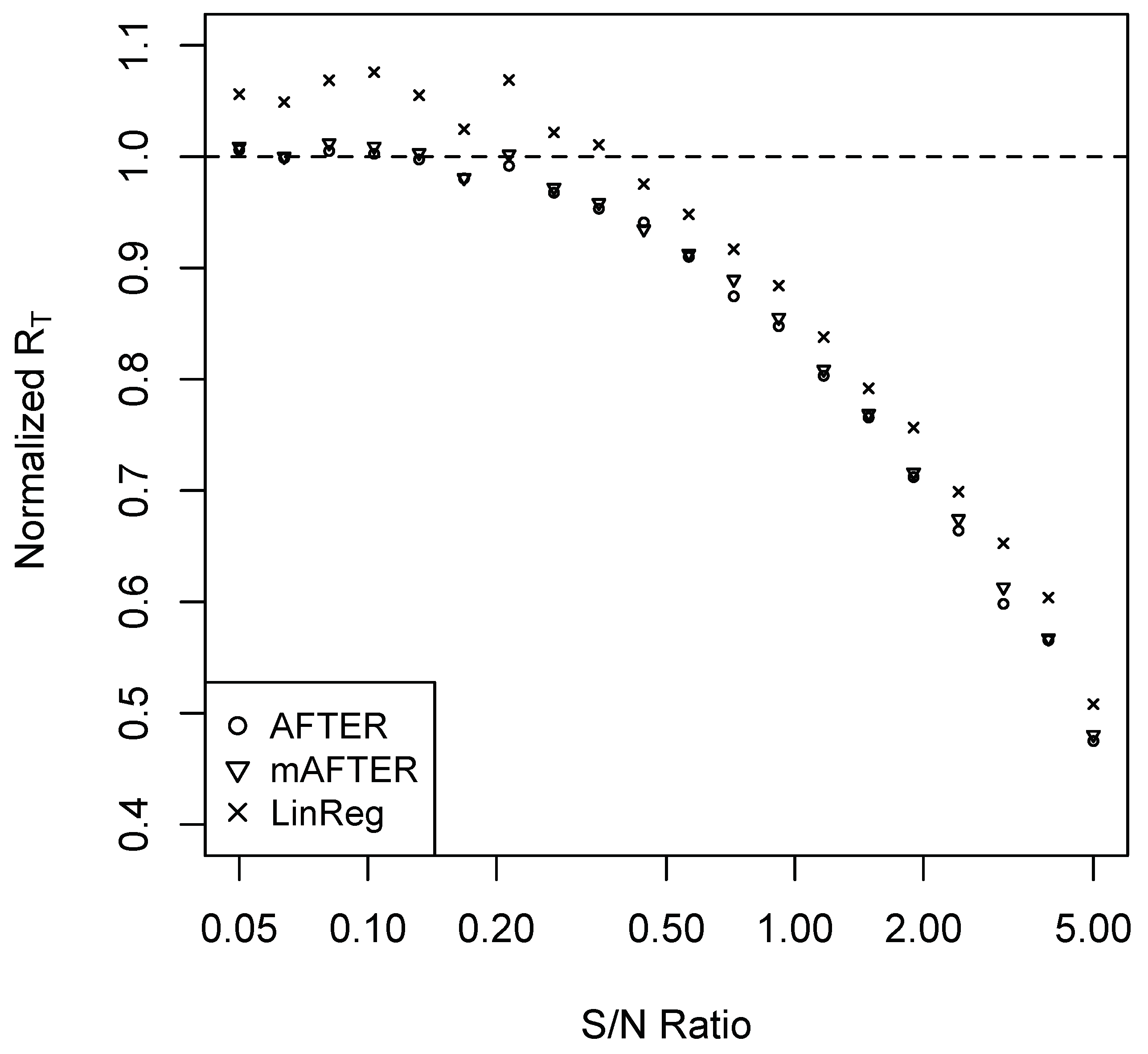
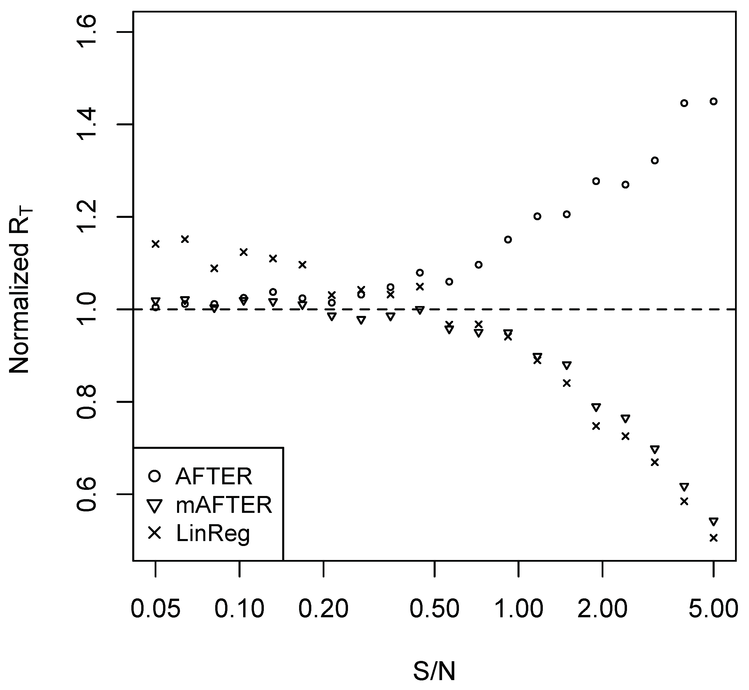
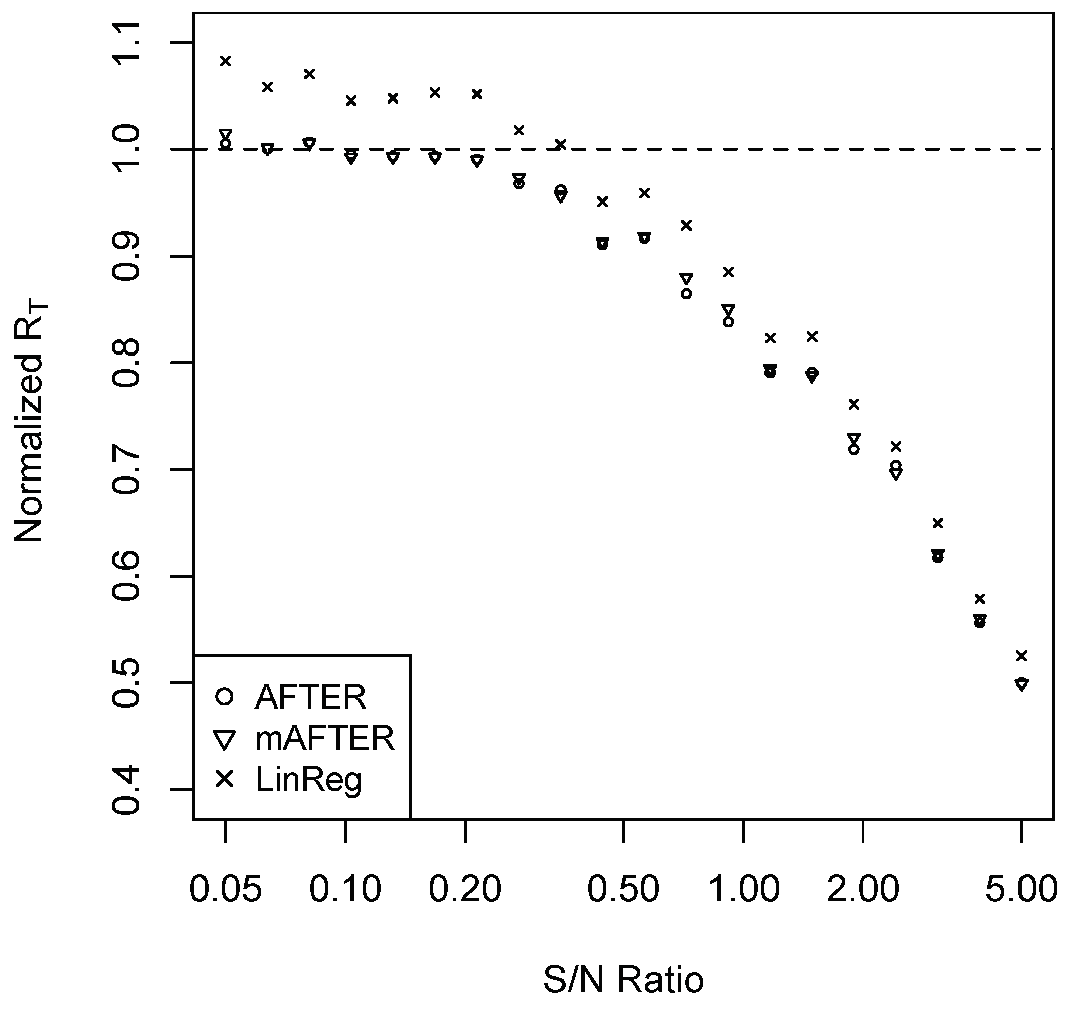
To confirm that the mAFTER strategy can mitigate the “puzzles” illustrated in the previous section, we repeated the simulation studies of Case 1 and Case 2 and summarize the results in Figure 3 and Figure 4, respectively. In Case 1, mAFTER correctly tracked the performance of AFTER. In Case 2, when S/N was relatively large (>0.5), mAFTER took advantage of the opportunity to improve over the original individual forecasts and performed very close to LinReg; when S/N was relatively small (<0.5), mAFTER behaved very similarly to SA and reduced the relatively heavy estimation error by LinReg. We also performed the simulation with information variables under AR(1) as (4); the results are summarized in Figure A3 and Figure A4 in the Appendix A, which show similar patterns as that of Figure 3 and Figure 4. Rather than relying on SA, a “sophisticated” combining strategy like mAFTER can be an appealingly safe method that, to some extent, mitigates FCP.
Note that mAFTER is a rather general forecast combination strategy. In the first step of the strategy, the analyst can choose their own way of generating new candidate forecasts (not necessarily restricted to AFTER and LinReg), as long as they include SA, representative methods for the CFA scenario, and representative methods for the CFI scenario. AFTER and LinReg were simply chosen in our study as convenient representatives. We also demonstrate the performance of the mAFTER strategy in the real data example in Section 9.
6. Is SA Really Robust?
The SA has been praised for being robust among the top performers relative to other forecast combination methods. It is obvious that SA cannot be robust in the traditional statistical sense: even a single really bad candidate can damage the performance of the combined forecast to an arbitrarily worse position. A more interesting question is to assess the robustness of SA in practically relevant settings.
The previous two sections showed that SA is not always robust in terms of its relative performance when dealing with the two different scenarios. In this section, we show that SA is not robust even in the loose sense when new forecast candidates are added to the candidate pool, especially if the new candidates have only redundant information with respect to the original candidate pool. In contrast, the AFTER-type combining methods can be rather robust against adding poor or redundant candidate forecasts. Here, we consider the following three cases.
- Case 3.
- Suppose a new information variable has the same distribution as and is independent of , , and . A new candidate forecast joins the candidate pool in Case 2, where is obtained from OLS estimation with historical data.
- Case 4.
- A new candidate forecast identical to Forecast 2 joins the candidate pool in Case 2.
- Case 5.
- A new candidate forecast is generated using a transformed information variable , where is obtained from OLS estimation with historical data. This new forecast joins the candidate pool in Case 2.
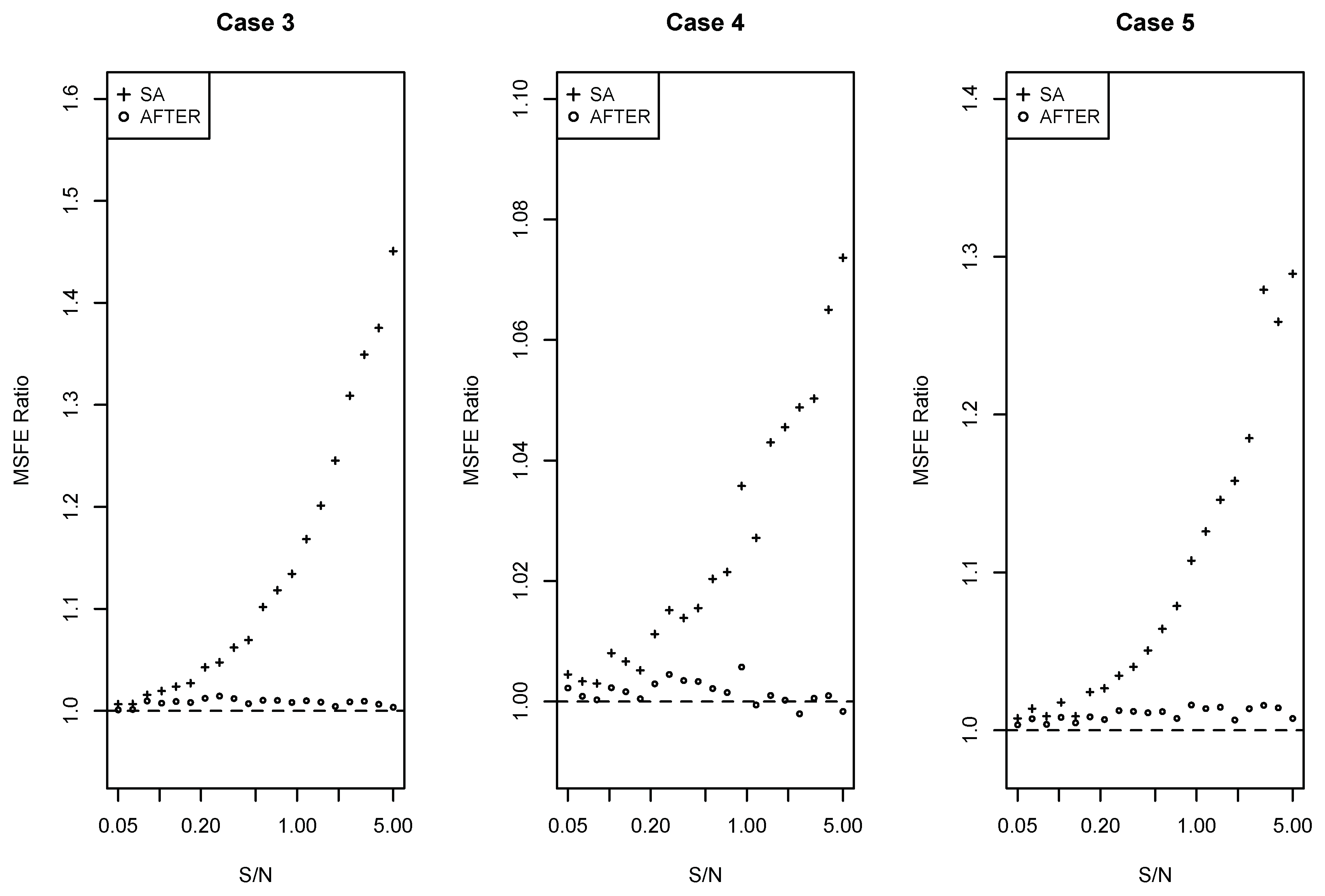
Note that the new candidate in Case 3 is a very poor forecast, while the new candidates in Case 4 and Case 5 contain a subset of the information variables. In all of the cases above, no new information is added to the candidate pool. Following the same simulation setting as Case 2, we focused on SA and AFTER and computed the ratio between the MSFE after adding the new candidate and the MSFE in Case 2. Figure 5 shows that the performance of AFTER remained almost the same, while the performance of SA worsened after adding the non-informative or redundant candidate forecasts.
7. Improper Weighting Formulas: A Source of the FCP Revisited
Generally speaking, the popular forecast combination methods often implicitly assume that the time series and/or the forecast errors are stationary. It is expected in theory that they should perform well if we have access to long enough historical data. In practice, however, such derived weighting formulas can often be unsuitable when the DGP changes and the candidate forecasts cannot adjust quickly to the new reality. For example, it is often believed that structural breaks can unexpectedly happen, making the relative performance of the candidate forecasts unstable and giving us the impression that SA performs well.
Next, we use a Monte Carlo example to illustrate the FCP under structural breaks. Rather than assuming deterministic shifts in information variables (Hendry and Clements 2004), we considered breaks in the DGP dynamics:
where the coefficients () are randomly generated from the uniform distribution on and ’s are . Here, structural breaks happen at and . The candidate forecast models are autoregressions from Lag 1 to Lag 6, and we apply SA, BG, LinReg, and AFTER to generate the combined forecasts. The simulation was repeated 100 times, and the last 100 time points served as the evaluation period to obtain the average forecast risk. For comparison, we considered the BG, LinReg, and AFTER methods with estimation rolling window size or 40, meaning only the most recent observations were used to estimate the weights for each forecast. The results are summarized in Table 1. The average forecast risk was normalized with respect to SA, and the numbers in parentheses are standard errors.
We can see from Table 1 that all three standard combining methods, when finding weights using all historical data, underperformed compared to SA due to the unstable relative performance of candidate forecasts. As we shrank the estimation window size to the most recent 40 and 20 time points, BG and AFTER achieved better performance than SA, while the performance of LinReg worsened. This result can be understood by noting that there are two opposing factors when we shrink the weight estimation window. When using only the most recent forecasts, we decreased the bias of the weighting formula supported by the old data, but simultaneously increased the variance of the estimated weight. Among the three methods considered, the estimation error factor dominated for LinReg. On the other hand, AFTER was not designed to target aggressively the optimal weight, thus benefiting more from the shrinking rolling window.
Due to the complex impact of structural breaks on forecast combination methods, it is arguably true that the focus should be made on how to detect the problem (e.g., Altissimo and Corradi 2003; Davis et al. 2006) and how to come up with new combining forms accordingly (e.g., using the most recent observations to avoid an improper weighting formula). However, proper identification of structural breaks can be difficult to achieve in practice, and this example shows that in the presence of structural breaks, the relative performance of SA was not always robust compared to BG and AFTER with naively-chosen rolling windows.
8. Linking Forecast Model Screening to FCP
In empirical studies, the candidate forecasting models are often screened/selected in some way to generate a smaller set of candidates for combining. As is demonstrated in Case 3 of Section 6, the performance of SA was particularly susceptible to poorly-performing candidate models. Therefore, the common practice of model screening may contribute to improving the observed performance of SA.
Next, we illustrate the impact of screening with a Monte Carlo example. Let () be the p-dimensional information variable vector randomly generated from a multivariate normal distribution with mean and covariance , where and or 0.5. Consider a DGP with the linear model setting:
where coefficient and are with or 4. Under this setting, only the first seven variables in are important for , while the remaining variables are not.
If we assume that the analyst has full access to the information vector ’s, we may build linear models as the candidate forecasts with any subset of the information variables. If we select the best subset model with the right size using the ABC criterion (Yang 1999) or combine the subset regression models by proper adaptive combining methods (Yang 2001), the prediction risk can adaptively achieve the minimax optimality over soft and hard sparse function classes (Wang et al. 2014). Inspired by this result, we considered the following screening-and-combining approach. First, given the model size (that is, the number of information variables used in a candidate linear model), choose the best OLS model based on the residual sum of squares. Second, from the p models selected from the first step, find the best X% () of the models based on the ABC criterion. Note that the ABC criterion for a subset model with size r is , where n is the estimation sample size, is the fitted response, and can be replaced by the usual unbiased estimates of . The selected subset models after this two-step procedure were then used to build the candidate forecasts for combining. In simulation, the total time horizon was set to be 200. The screening procedures were applied to the first 100 observations, and the remaining models were used to build the candidate forecasts for the latter 100 time points. Different forecast combination methods were applied, and their performance is evaluated using the last 50 observations. The simulation was repeated 100 times, and the normalized average forecast risk (relative to SA) is summarized in Table 2.
Table 2 shows that AFTER outperformed all the other competitors including SA in this case study. This is consistent with our understanding of a typical CFA scenario, under which AFTER is the proper choice of combining method. However, as we decreased X and selected smaller sets of candidate forecasts for combining, the performance of SA gradually approached that of AFTER. LinReg, which is not a proper choice under the CFA scenario, appeared to underperform compared to SA. As X decreased, LinReg became less subject to weight estimation error, and the performance of LinReg improved relative to SA.
From this example, we can see that the performance of SA was not robust to the degree of screening. Generally, it can be a challenging task to ensure an optimal screening to make SA perform well. Without a good screening/selection rule, it leaves too much freedom for the analyst to make reliable decisions. We note that a possible solution is to first create new candidate forecasts (e.g., forecasts generated by linear regression methods) to utilize most or all of the important information, and then the roles of a good screening/selection rule can be played by applying the multi-level AFTER approach (introduced in Section 5) on both the original forecasts and the combined forecasts to reduce the influence of the poorly-performing or redundant forecasts.
9. Real Data Evaluation
In this section, we study the U.S. SPF (Society of Professional Forecasters) dataset to evaluate SA and the mAFTER strategy. This dataset is a quarterly survey on macroeconomic forecasts in the United States. Lahiri et al. (2013) nicely handled the missing forecasts by adopting two missing forecast imputation strategies known as the regression imputation (REG-Imputed) and the simple average imputation (SA-Imputed) to generate the complete panels (see also the updates in Lahiri et al. 2017). As pointed out by Lahiri et al. (2013), the change of the data administration agency in 1990 and the subsequently shifting missing data pattern made it difficult to use the entire data period for meaningful evaluation. In this empirical illustration, we adopted this missing forecast imputation and the forecast selection strategies; we used the datasets shared by Lahiri et al. (2013) on the period from 1968 to 1990 (pre-1990 period) and the period from 2000 to 2013 (post-2000 period) to evaluate the performance of the mAFTER strategy. Note that an alternative and convenient way to handle missing data was also discussed in Matsypura et al. (2018) for certain covariance-based combination methods.
Three macroeconomic variables are considered: seasonally-adjusted annual rate of change for GDP price deflator (PGDP), growth rate of real GDP (RGDP), and quarterly average of the monthly unemployment rate (UNEMP). For the pre-1990 period, the datasets for RGDP and PGDP had 14 candidate forecasts, and the datasets for UNEMP had 13 candidate forecasts. For the post-2000 period, all the datasets had 19 candidate forecasts. Each forecast provided g-quarter-ahead () forecasting. We applied SA, AFTER, BG, LinReg, and mAFTER to each SPF dataset of a macroeconomic variable with a given missing forecast imputation method. Each forecast combination method used the first 20 time points to build up the initial weights, and the remaining time points were used to calculate the normalized MSFE of each method relative to SA. By taking the average over the four MSFEs that correspond to the 1,2,3,4-quarter ahead forecasting, we summarize the performance of different combining methods in Table 3 for the pre-1990 period and Table 4 for the post-2000 period.
From Table 3 for the pre-1990 period, although AFTER performed quite differently with different target macroeconomic variables, the mAFTER strategy delivered overall robust performance for all three variables. For PGDP, AFTER performed the best and beat SA by as much as 10%. Using mAFTER successfully maintained this advantage over SA. For RGDP, while SA and BG beat AFTER by up to 13%, mAFTER successfully pulled the performance to be within 3% of SA. Finally, for the UNEMP variable, SA, BG, and AFTER all performed very similarly with no more than a 3% difference, and the performance of mAFTER did not deviate much from either SA or AFTER. The LinReg method performed poorly for all three target variables. It is interesting to note from Figure 6 that for both the PGDP and RGDP variables, the largest performance difference between SA and AFTER was found in the one-quarter ahead forecasting; in each case, mAFTER robustly matched the better of SA and AFTER.
Like the pre-1990 period, we observe from Table 4 for the post-2000 period that AFTER continued to exhibit very different performance across different target variables, while mAFTER remained relatively robust. In particular, for the UNEMP variable, AFTER performed well compared to SA by reducing the averaged MSFEs by as much as 10%; satisfactorily, mAFTER largely maintained the performance advantage of AFTER. On the other hand, for the PGDP variable, the averaged MSFEs for the plain-vanilla AFTER were about 15% higher than those of SA and BG, but mAFTER successfully improved the performance of AFTER to be within 3% of SA. For the RGDP variable, SA, BG, and AFTER (including mAFTER) performed similarly with no more than a 3% difference. These observed empirical results coincided with the robustness expectation from Proposition 1 on the mAFTER strategy.
10. Conclusions
Inspired by the seemingly mysterious FCP, we attempted to offer some explanations of why the puzzle can occur and investigated when a sophisticated combining method can work well compared to SA. Our study illustrated that the following reasons may contribute to the puzzle.
First, estimation error is known to be an important source of FCP. Both theoretical and empirical evidence show that a relatively small sample size may prevent some combining methods from reliably estimating the optimal weight. Second, FCP can appear if we apply a combining method without consideration of the underlying data scenarios. The relative performance of SA may depend heavily on which scenario is more proper for the data. Third, the weighting formula of the combining methods is not always appropriate for the data, because structural breaks and shocks can unexpectedly happen. The weighting formula obtained by sophisticated methods may not adjust fast enough to the reality, resulting in performance less stable than SA. Fourth, candidate forecasts are often screened in some way so that the remaining forecasts used for combining tend to have similar performance, and SA may tend to work well in such cases. However, SA can be sensitive to the screening process, and enlarging the pool of candidates may benefit other combination methods; therefore, empirical observations that SA works well after model screening should be taken with a grain of salt. Fifth, there may be publication bias in that people tend to report the existence of FCP when SA gives good empirical results, but may not emphasize the performance of SA when it gives mediocre results.
Regarding the first two reasons above, it is not hard to find data and build candidate forecasts in a certain way to favor a sophisticated or simple method. Under the CFA scenario, the estimation price can be mitigated by applying combining methods designed to target the performance of the best candidate forecast. Under the CFI scenario, past literature has properly pointed out the potentially high cost of estimation error when targeting the optimal weight, but we do not necessarily have to pay a very high cost. A carefully-designed mAFTER strategy can perform aggressively to target the optimal weight when information is sufficient to support exploiting the optimal weighting and perform conservatively like SA when the degree of estimation error is high. mAFTER can also intelligently perform according to the underlying scenario (CFA or CFI), circumventing the “puzzle” caused by improperly-chosen combining methods. Lastly, it is worth noting that FCP, a classical issue that emerged decades ago, remains to be a relevant topic and testbed for further understanding of important forecast combination methods; it would be interesting to exploit the proposed ideas and strategies here to the new post-M4 competition settings (Makridakis et al. 2018), and we leave comprehensive exploration efforts for future investigation.
Author Contributions
This is a collaborative project. All authors contributed to the paper equally. The proofs are done by W.Q.
Funding
W. Qian’s research is partially supported by the NSF Grant DMS-1916376 and by the JPMC Faculty Fellowship.
Acknowledgments
We thank Kajal Lahiri for sharing the imputed U.S. SPF datasets and Jeremy Piger for helpful comments. We would also like to thank the Editors and two anonymous referees for comments that helped to improve this manuscript significantly.
Conflicts of Interest
The authors declare no conflict of interest.
Appendix A
Appendix A.1. Assumptions of Proposition 1
The following two assumptions are sufficient regularity conditions for Propostion 1. Note that Assumption A1 is satisfied if we truncate the candidate forecasts to have certain lower and upper bounds. Assumption A2 is satisfied if the conditional distributions of the random noise are sub-Gaussian.
Assumption A1.
There exists a positive constant M such that the candidate forecasts satisfy with probability one that:
Assumption A2.
There exist a constant and continuous functions on such that for every and ,
with probability one.
Appendix A.2. Propositions and Proofs
Proposition A1.
Under the settings of Case 1, the average forecast risk of Forecast 1 relative to the SA satisfies:
In addition, if we consider the weight vectors in , the asymptotic optimal combination weight satisfies:
Proposition A2.
Under the settings of Case 2, the average forecast risk of Forecast 1 relative to the SA satisfies:
In addition, the asymptotic optimal combination weight under the restriction satisfies:
where:
in particular, if and , then . The asymptotic optimal combination weight without the restriction satisfies:
in particular, if and , then .
The proof of Proposition A1 is similar to that of Proposition A2. In the following, we provide a sketch for the proof of Proposition A2.
Proof of Proposition A2.
Let , and be the point-wise forecast risks at time T for Forecast 1, Forecast 2, and the combined forecast, respectively. We will first verify that under the restriction ,
where is the estimated covariate standard deviation () and is the estimated covariate correlation.
First, we have:
The expression for can be derived similarly. For , we have:
where:
With tedious algebra, it is not hard to show that:
Together with the previous displays, we verify Formula (A4) for . Subsequently, (A1) can be verified by noting that the ’s are normally distributed and that as (). Then, we can apply the Karush–Kuhn–Tucker (KKT) conditions for minimizing with the constraint on to obtain (A2) straightforwardly.
When there is no restriction on , tedious derivation similar to above for gives that:
Consequently, with first-order optimality conditions, the display above implies (A3). This completes the proof of Proposition A2. □
Appendix A.3. Additional Numerical Results
In the following, we provide the plots for the average forecast risk of different forecast combination methods when the information variables have the AR(1) assumptions. These plots in Figure A1, Figure A2, Figure A3 and Figure A4 appear to give similar patterns as those of Figure 1, Figure 2, Figure 3 and Figure 4.
Figure A1.
(Case 1) Comparing the average forecast risk of different forecast combination methods with AR(1) information variables (the dashed line represents the SA baseline; the x-axis is in logarithmic scale).
Figure A1.
(Case 1) Comparing the average forecast risk of different forecast combination methods with AR(1) information variables (the dashed line represents the SA baseline; the x-axis is in logarithmic scale).

Figure A2.
(Case 2) Comparing the average forecast risk of different forecast combination methods with AR(1) information variables (the dashed line represents the SA baseline; the x-axis is in logarithmic scale).
Figure A2.
(Case 2) Comparing the average forecast risk of different forecast combination methods with AR(1) information variables (the dashed line represents the SA baseline; the x-axis is in logarithmic scale).

Figure A3.
(Case 1) Performance of mAFTER under the adaptation scenario with AR(1) information variables (the dashed line represents the SA baseline; the x-axis is in logarithmic scale).
Figure A3.
(Case 1) Performance of mAFTER under the adaptation scenario with AR(1) information variables (the dashed line represents the SA baseline; the x-axis is in logarithmic scale).

Figure A4.
(Case 2) Performance of mAFTER under improvement scenario with AR(1) information variables (the dashed line represents the SA baseline; the x-axis is in logarithmic scale).
Figure A4.
(Case 2) Performance of mAFTER under improvement scenario with AR(1) information variables (the dashed line represents the SA baseline; the x-axis is in logarithmic scale).

References
- Altissimo, F., and V. Corradi. 2003. Strong rules for detecting the number of breaks in a time series. Journal of Econometrics 117: 207–44. [Google Scholar] [CrossRef]
- Ando, T., and K.-C. Li. 2014. A model-averaging approach for high-dimensional regression. Journal of the American Statistical Association 109: 254–65. [Google Scholar] [CrossRef]
- Bates, J. M., and C. W. J. Granger. 1969. The combination of forecasts. Operation Research Quarterly 20: 451–68. [Google Scholar] [CrossRef]
- Bordignon, Silvano, Derek W. Bunn, Francesco Lisi, and Fany Nan. 2013. Combining day-ahead forecasts for British electricity prices. Energy Economics 35: 88–103. [Google Scholar] [CrossRef] [Green Version]
- Buckland, Stephen T., Kenneth P. Burnham, and Nicole H. Augustin. 1997. Model selection: an integral part of inference. Biometrics 53: 603–18. [Google Scholar] [CrossRef]
- Chen, Jia, Degui Li, Oliver Linton, and Zudi Lu. 2018. Semiparametric ultra-high dimensional model averaging of nonlinear dynamic time series. Journal of the American Statistical Association 113: 919–32. [Google Scholar] [CrossRef]
- Chen, Longmei, Alan T. K. Wan, Geoffrey Tso, and Xinyu Zhang. 2018. A model averaging approach for the ordered probit and nested logit models with applications. Journal of Applied Statistics 45: 3012–52. [Google Scholar] [CrossRef]
- Cheng, Gang, and Yuhong Yang. 2015. Forecast combination with outlier protection. International Journal of Forecasting 31: 223–37. [Google Scholar] [CrossRef]
- Cheng, Tzu-Chang F., Ching-Kang Ing, and Shu-Hui Yu. 2015. Toward optimal model averaging in regression models with time series errors. Journal of Econometrics 189: 321–34. [Google Scholar] [CrossRef]
- Cheng, Xu, and Bruce E. Hansen. 2015. Forecasting with factor-augmented regression: A frequentist model averaging approach. Journal of Econometrics 186: 280–93. [Google Scholar] [CrossRef]
- Claeskens, Gerda, Jan R. Magnus, Andrey L. Vasnev, and Wendun Wang. 2016. The forecast combination puzzle: A simple theoretical explanation. International Journal of Forecasting 32: 754–62. [Google Scholar] [CrossRef]
- Clemen, Robert T. 1989. Combining forecasts: A review and annotated bibliography. International Journal of Forecasting 5: 559–83. [Google Scholar] [CrossRef]
- Clemen, Robert T., Allan H. Murphy, and Robert L. Winkler. 1995. Screening probability forecasts: contrasts between choosing and combining. International Journal of Forecasting 11: 133–45. [Google Scholar] [CrossRef]
- Clemen, Robert T., and Robert L. Winkler. 1986. Combining economic forecasts. Journal of Business & Economic Statistics 4: 39–46. [Google Scholar]
- Davis, Richard A., Thomas C. M. Lee, and Gabriel A. Rodriguez-Yam. 2006. Structural break estimation for nonstationary time series models. Journal of the American Statistical Association 101: 223–39. [Google Scholar] [CrossRef]
- De Luca, Giuseppe, Jan R. Magnus, and Franco Peracchi. 2018. Weighted-average least squares estimation of generalized linear models. Journal of Econometrics 204: 1–17. [Google Scholar] [CrossRef] [Green Version]
- Diebold, Francis X., and Peter Pauly. 1990. The use of prior information in forecast combination. International Journal of Forecasting 6: 503–8. [Google Scholar] [CrossRef]
- Elliott, Gayle. 2011. Averaging and the Optimal Combination of Forecasts. Technical Report, UCSD Working Paper. San Diego: UCSD. [Google Scholar]
- Fan, Jianqing, and Jinchi Lv. 2008. Sure independence screening for ultrahigh dimensional feature space. Journal of the Royal Statistical Society: Series B(Statistical Methodology) 70: 849–911. [Google Scholar] [CrossRef] [Green Version]
- Fan, Jianqing, and Rui Song. 2010. Sure independence screening in generalized linear models with NP-dimensionality. The Annals of Statistics 38: 3567–604. [Google Scholar] [CrossRef]
- Forte, Anabel, Gonzalo Garcia-Donato, and Mark Steel. 2018. Methods and tools for bayesian variable selection and model averaging in normal linear regression. International Statistical Review 86: 237–58. [Google Scholar] [CrossRef]
- Friedman, Jerome, Trevor Hastie, and Robert Tibshirani. 2000. Additive logistic regression: a statistical view of boosting. The Annals of Statistics 28: 337–407. [Google Scholar] [CrossRef]
- Friedman, Jerome. 2001. Greedy function approximation: a gradient boosting machine. The Annals of Statistics 29: 1189–232. [Google Scholar] [CrossRef]
- Garcia-Donato, G., and M. A. Martinez-Beneito. 2013. On sampling strategies in bayesian variable selection problems with large model spaces. Journal of the American Statistical Association 108: 340–52. [Google Scholar] [CrossRef]
- Genre, Veronique, Geoff Kenny, Aidan Meyler, and Allan Timmermann. 2013. Combining expert forecasts: Can anything beat the simple average? International Journal of Forecasting 29: 108–21. [Google Scholar] [CrossRef]
- Gibbs, Christopher, and Andrey L. Vasnev. 2017. Conditionally Optimal Weights and Forward-Looking Approaches to Combining Forecasts. SSRN 2919117. Available online: https://papers.ssrn.com/sol3/papers.cfm?abstract_id=2919117 (accessed on 1 August 2019).[Green Version]
- Granger, Clive W. J., and Ramu Ramanathan. 1984. Improved methods of combining forecasts. Journal of Forecasting 3: 197–204. [Google Scholar] [CrossRef]
- Hendry, David F., and Michael P. Clements. 2004. Pooling of forecasts. The Econometrics Journal 7: 1–31. [Google Scholar] [CrossRef] [Green Version]
- Hoeting, Jennifer A., David Madigan, Adrian E. Raftery, and Chris T. Volinsky. 1999. Bayesian model averaging: A tutorial. Statistical Science 14: 382–401. [Google Scholar]
- Hsiao, Cheng, and Shui-Ki Wan. 2014. Is there an optimal forecast combination? Journal of Econometrics 178: 294–309. [Google Scholar] [CrossRef]
- Huang, Huiyu, and Tae-Hwy Lee. 2010. To combine forecasts or to combine information? Econometric Reviews 29: 534–70. [Google Scholar] [CrossRef]
- Ing, Ching-Kang, and Tze Leung Lai. 2011. A stepwise regression method and consistent model selection for high-dimensional sparse linear models. Statistica Sinica 21: 1473–513. [Google Scholar] [CrossRef]
- Kourentzes, Nikolaos, Devon Barrow, and Fotios Petropoulos. 2019. Another look at forecast selection and combination: Evidence from forecast pooling. International Journal of Production Economics 209: 226–35. [Google Scholar] [CrossRef]
- Lahiri, Kajal, Huaming Peng, and Yongchen Zhao. 2013. Machine Learning and Forecast Combination in Incomplete Panels. Semantic Scholar and SSRN 2359523. Available online: https://pdfs.semanticscholar.org/ae57/a60eab315a7811381a24c52512688417096e.pdf (accessed on 1 August 2019).[Green Version]
- Lahiri, Kajal, Huaming Peng, and Yongchen Zhao. 2017. Online learning and forecast combination in unbalanced panels. Econometric Reviews 36: 257–88. [Google Scholar] [CrossRef]
- Lan, Wei, Yingying Ma, Junlong Zhao, Hansheng Wang, and Chih-Ling Tsai. 2019. Sequential model averaging for high dimensional linear regression models. Statistica Sinica. accepted. [Google Scholar]
- Magnus, Jan R., and Giuseppe De Luca. 2016. Weighted-average least squares (WALS): A survey. Journal of Economic Surveys 30: 117–48. [Google Scholar] [CrossRef]
- Magnus, Jan R., Wendun Wang, and Xinyu Zhang. 2016. Weighted-average least squares prediction. Econometric Reviews 35: 1040–74. [Google Scholar] [CrossRef]
- Makridakis, Spyros, Evangelos Spiliotis, and Vassilios Assimakopoulos. 2018. The M4 competition: Results, findings, conclusion and way forward. International Journal of Forecasting 34: 802–8. [Google Scholar] [CrossRef]
- Matsypura, Dmytro, Ryan Thompson, and Andrey L. Vasnev. 2018. Optimal selection of expert forecasts with integer programming. Omega 78: 165–75. [Google Scholar] [CrossRef]
- Qian, Wei, Wending Li, Yasuhiro Sogawa, Ryohei Fujimaki, Xitong Yang, and Ji Liu. 2018. An interactive greedy approach to group sparsity in high dimensions. Technometrics 61: 409–21. [Google Scholar] [CrossRef]
- Rolling, Craig A., Wei Qian, Gang Cheng, and Yuhong Yang. 2019. Identifying the proper goal of forecast combination. Preprint. [Google Scholar]
- Rolling, Craig A., Yuhong Yang, and Dagmar Velez. 2018. Combining estimates of conditional treatment effects. Econometric Theory, 1–22. [Google Scholar] [CrossRef]
- Smith, Jeremy, and Kenneth F. Wallis. 2009. A simple explanation of the forecast combination puzzle. Oxford Bulletin of Economics and Statistics 71: 331–55. [Google Scholar] [CrossRef]
- Steel, Mark F. 2011. Bayesian model averaging and forecasting. Bulletin of EU and US Inflation and Macroeconomic Analysis 200: 30–41. [Google Scholar]
- Steel, Mark F. 2014. Bayesian model averaging. In Wiley StatsRef: Statistics Reference Online. Hoboken: John Wiley & Sons, Ltd., pp. 1–7. [Google Scholar]
- Stock, James H., and Mark W. Watson. 1998. A Comparison of Linear and Nonlinear Univariate Models for Forecasting Macroeconomic Time Series. Technical Report, National Bureau of Economic Research. Cambridge: National Bureau of Economic Research. [Google Scholar]
- Stock, James H., and Mark W. Watson. 2004. Combination forecasts of output growth in a seven-country data set. Journal of Forecasting 23: 405–30. [Google Scholar] [CrossRef]
- Tibshirani, Robert. 1996. Regression shrinkage and selection via the lasso. Journal of the Royal Statistical Society: Series B (Methodological) 58: 267–88. [Google Scholar] [CrossRef]
- Timmermann, Allan. 2006. Forecast combinations. Handbook of Economic Forecasting 1: 135–96. [Google Scholar]
- Wan, Alan T.K., Xinyu Zhang, and Guohua Zou. 2010. Least squares model averaging by mallows criterion. Journal of Econometrics 156: 277–83. [Google Scholar] [CrossRef]
- Wang, Zhan, Sandra Paterlini, Fuchang Gao, and Yuhong Yang. 2014. Adaptive minimax regression estimation over sparse ℓq-hulls. Journal of Machine Learning Research 15: 1675–711. [Google Scholar]
- Winkler, Robert L., and Spyros Makridakis. 1983. The combination of forecasts. Journal of the Royal Statistical Society, Series A 146: 150–57. [Google Scholar] [CrossRef]
- Yang, Yuhong. 1999. Model selection for nonparametric regression. Statistica Sinica 9: 475–99. [Google Scholar]
- Yang, Yuhong. 2001. Adaptive regression by mixing. Journal of the American Statistical Association 96: 574–88. [Google Scholar] [CrossRef]
- Yang, Yuhong. 2004. Combining forecasting procedures: Some theoretical results. Econometric Theory 20: 176–222. [Google Scholar] [CrossRef]
- Yang, Yi, Wei Qian, and Hui Zou. 2018. Insurance premium prediction via gradient tree-boosted Tweedie compound Poisson models. Journal of Business & Economic Statistics 36: 456–70. [Google Scholar]
- Yuan, Zheng, and Yuhong Yang. 2005. Combining linear regression models. Journal of the American Statistical Association 100: 1202–14. [Google Scholar] [CrossRef]
- Zhang, Tong. 2011. Adaptive forward-backward greedy algorithm for learning sparse representations. IEEE Transactions on Information Theory 57: 4689–708. [Google Scholar] [CrossRef]
- Zhang, Xinyu, Zudi Lu, and Guohua Zou. 2013. Adaptively combined forecasting for discrete response time series. Journal of Econometrics 176: 80–91. [Google Scholar] [CrossRef]
- Zhang, Xinyu, Dalei Yu, Guohua Zou, and Hua Liang. 2016. Optimal model averaging estimation for generalized linear models and generalized linear mixed-effects models. Journal of the American Statistical Association 111: 1775–90. [Google Scholar] [CrossRef]
- Zhang, Xinyu, and Jihai Yu. 2018. Spatial weights matrix selection and model averaging for spatial autoregressive models. Journal of Econometrics 203: 1–18. [Google Scholar] [CrossRef]
- Zhu, Rong, Alan T.K. Wan, Xinyu Zhang, and Guohua Zou. 2018. A Mallows-type model averaging estimator for the varying-coefficient partially linear model. Journal of the American Statistical Association 114: 882–92. [Google Scholar] [CrossRef]
- Zou, Hui. 2006. The adaptive lasso and its oracle properties. Journal of the American Statistical Association 101: 1418–29. [Google Scholar] [CrossRef]
Figure 1.
(Case 1) Comparing the average forecast risk of different forecast combination methods (the dashed line represents the simple average (SA) baseline; the x-axis is in logarithmic scale). BG, Bates and Granger; LinReg, linear regression.
Figure 1.
(Case 1) Comparing the average forecast risk of different forecast combination methods (the dashed line represents the simple average (SA) baseline; the x-axis is in logarithmic scale). BG, Bates and Granger; LinReg, linear regression.

Figure 2.
(Case 2) Comparing the average forecast risk of different forecast combination methods (the dashed line represents the SA baseline; the x-axis is in the logarithmic scale).
Figure 2.
(Case 2) Comparing the average forecast risk of different forecast combination methods (the dashed line represents the SA baseline; the x-axis is in the logarithmic scale).

Figure 3.
(Case 1) Performance of mAFTER under the adaptation scenario (the dashed line represents the SA baseline; the x-axis is in the logarithmic scale).
Figure 3.
(Case 1) Performance of mAFTER under the adaptation scenario (the dashed line represents the SA baseline; the x-axis is in the logarithmic scale).

Figure 4.
(Case 2) Performance of mAFTER under the improvement scenario (the dashed line represents the SA baseline; the x-axis is in logarithmic scale).
Figure 4.
(Case 2) Performance of mAFTER under the improvement scenario (the dashed line represents the SA baseline; the x-axis is in logarithmic scale).

Figure 5.
Studying the robustness of SA against adding new candidate forecasts.

Figure 6.
Comparing normalized MSFEs of different forecast combination methods with REG-Imputed SPF datasets (pre-1990 period). Left panel: PGDP variable. Right panel: RGDP variable. For each method, the bars from left to right represent 1-, 2-, 3-, and 4-quarter ahead forecasting results, respectively. The dashed line represents the SA baseline.


Table 1.
Comparing the normalized average forecast risk of different combination methods under structural breaks.
Table 1.
Comparing the normalized average forecast risk of different combination methods under structural breaks.
| SA | LinReg | BG | AFTER | |
|---|---|---|---|---|
| standard | 1.000 | 1.026 (0.011) | 1.005 (0.003) | 1.047 (0.010) |
| 1.000 | 1.060 (0.033) | 0.992 (0.002) | 0.991 (0.009) | |
| 1.000 | 1.64 (0.42) | 0.980 (0.003) | 0.952 (0.007) |
Table 2.
Comparing the normalized average forecast risk of different forecast combination methods after the procedure of screening and selecting the best X% models for subsequent forecast combining.
Table 2.
Comparing the normalized average forecast risk of different forecast combination methods after the procedure of screening and selecting the best X% models for subsequent forecast combining.
| Best X% | 10% | 20% | 40% | 60% | 80% |
|---|---|---|---|---|---|
| , | |||||
| AFTER | 0.998 | 0.989 | 0.966 | 0.951 | 0.945 |
| BG | 1.000 | 0.999 | 0.997 | 0.997 | 0.996 |
| LinReg | 1.017 | 1.024 | 1.056 | 1.098 | 1.151 |
| , | |||||
| AFTER | 0.996 | 0.990 | 0.968 | 0.956 | 0.951 |
| BG | 1.000 | 0.998 | 0.997 | 0.997 | 0.996 |
| LinReg | 1.013 | 1.024 | 1.043 | 1.095 | 1.159 |
| , | |||||
| AFTER | 0.994 | 0.987 | 0.984 | 0.981 | 0.974 |
| BG | 0.999 | 0.998 | 0.998 | 0.998 | 0.997 |
| LinReg | 1.002 | 1.012 | 1.056 | 1.101 | 1.163 |
| , | |||||
| AFTER | 0.995 | 0.990 | 0.976 | 0.969 | 0.961 |
| BG | 1.000 | 0.999 | 0.998 | 0.997 | 0.997 |
| LinReg | 1.004 | 1.010 | 1.030 | 1.086 | 1.136 |
Table 3.
Comparing the performance of forecast combination methods with the Society of Professional Forecasters (SPF) datasets (pre-1990 period). Values shown are normalized MSFEs averaged over 1-, 2-, 3-, and 4-quarter-ahead forecasting. mAFTER, multi-level AFTER; RGDP, growth rate of real GDP; UNEMP, quarterly average of the monthly unemployment rate; REG, regression.
| Target Variable | SA | LinReg | BG | AFTER | mAFTER |
|---|---|---|---|---|---|
| REG-imputed | |||||
| PGDP | 1.00 | 1.88 | 0.95 | 0.90 | 0.90 |
| RGDP | 1.00 | 1.64 | 1.00 | 1.11 | 1.01 |
| UNEMP | 1.00 | 1.79 | 0.99 | 0.98 | 0.98 |
| SA-imputed | |||||
| PGDP | 1.00 | 2.17 | 0.98 | 0.95 | 0.95 |
| RGDP | 1.00 | 1.83 | 1.00 | 1.13 | 1.03 |
| UNEMP | 1.00 | 1.69 | 0.99 | 0.97 | 0.98 |
Table 4.
Comparing the performance of the forecast combination methods with SPF datasets (post-2000 period). Values shown are normalized MSFEs averaged over 1-, 2-, 3-, and 4-quarter ahead forecasting.
Table 4.
Comparing the performance of the forecast combination methods with SPF datasets (post-2000 period). Values shown are normalized MSFEs averaged over 1-, 2-, 3-, and 4-quarter ahead forecasting.
| Target Variable | SA | LinReg | BG | AFTER | mAFTER |
|---|---|---|---|---|---|
| REG-imputed | |||||
| PGDP | 1.00 | 5.70 | 1.00 | 1.15 | 1.02 |
| RGDP | 1.00 | 6.55 | 1.00 | 1.03 | 1.02 |
| UNEMP | 1.00 | 1.03 | 0.95 | 0.90 | 0.91 |
| SA-imputed | |||||
| PGDP | 1.00 | 8.05 | 1.00 | 1.15 | 1.02 |
| RGDP | 1.00 | 3.03 | 1.02 | 1.03 | 1.02 |
| UNEMP | 1.00 | 1.01 | 0.96 | 0.92 | 0.93 |
© 2019 by the authors. Licensee MDPI, Basel, Switzerland. This article is an open access article distributed under the terms and conditions of the Creative Commons Attribution (CC BY) license (http://creativecommons.org/licenses/by/4.0/).
Share and Cite
MDPI and ACS Style
Qian, W.; Rolling, C.A.; Cheng, G.; Yang, Y. On the Forecast Combination Puzzle. Econometrics 2019, 7, 39. https://0-doi-org.brum.beds.ac.uk/10.3390/econometrics7030039
AMA Style
Qian W, Rolling CA, Cheng G, Yang Y. On the Forecast Combination Puzzle. Econometrics. 2019; 7(3):39. https://0-doi-org.brum.beds.ac.uk/10.3390/econometrics7030039
Chicago/Turabian StyleQian, Wei, Craig A. Rolling, Gang Cheng, and Yuhong Yang. 2019. "On the Forecast Combination Puzzle" Econometrics 7, no. 3: 39. https://0-doi-org.brum.beds.ac.uk/10.3390/econometrics7030039
Note that from the first issue of 2016, this journal uses article numbers instead of page numbers. See further details here.