Mahalanobis Distances on Factor Model Based Estimation


Department of Economics and Statistics, Linnaeus university, 351 95 Växjö, Sweden
Econometrics 2020, 8(1), 10; https://0-doi-org.brum.beds.ac.uk/10.3390/econometrics8010010
Submission received: 20 August 2019
/
Revised: 28 February 2020
/
Accepted: 2 March 2020
/
Published: 5 March 2020
Abstract
:A factor model based covariance matrix is used to build a new form of Mahalanobis distance. The distribution and relative properties of the new Mahalanobis distances are derived. A new type of Mahalanobis distance based on the separated part of the factor model is defined. Contamination effects of outliers detected by the new defined Mahalanobis distances are also investigated. An empirical example indicates that the new proposed separated type of Mahalanobis distances predominate the original sample Mahalanobis distance.
1. Introduction
The measurement of the distance between two individual observations is a fundamental topic in some research areas. The most commonly used statistics for the measurements are Euclidean distance and Mahalanobis distance (MD). By taking the covariance matrix into account, the MD is more suitable for the analysis of correlated data. Thus, MD has become one of the most commonly implemented tools for outlier detection since it was introduced by Mahalanobis (1936). Through decades of development, its usages are extended into a few broader applications, such as: assessing multivariate normality (Holgersson and Shukur 2001; Mardia 1974; Mardia et al. 1980), classification (Fisher 1940; Pavlenko 2003) and outlier detection (Mardia et al. 1980; Wilks 1963), etc.
However, as the number of variables increase, the estimation on an unconstrained covariance matrix becomes inefficient and computationally expensive, and so does the estimated sample MD. Thus, an efficient and easier method of estimating the covariance matrix is needed. This target can be achieved for some structured data. For instance, in factor–structured data, the correlated observations contain common information which can be represented into fewer variables by using dimension reduction tools, for example, factor model. The fewer variables are a linear combination of the original variable in the data set. The newly built factor model has the advantages of summarising the internal information of data and expressing it with much fewer latent factors in a linear model form with residuals. The idea of implement factor model on structured data is widely applied in different research areas. For example, in arbitrage pricing theory (Ross 1976), the asset return is assumed to follow a factor structure. In consumer theory, factor analysis shows that utility maximising could be described by at most three factors (Gorman et al. 1981; Lewbel 1991). In desegregate business cycle analysis, the factor model is used to identify the common and specific shocks that drive a country’s economy (Bai 2003; Gregory and Head 1999).
The robustness of factor model is also of substantial concern. Pison et al. (2003) proposed a robust version of factor model which is highly resistant to the outliers. Yuan and Zhong (2008) defined different types of outliers as good or bad leverage points. Their research set a criterion to distinguish different types of outliers based on evaluating the effects on the MLE and likelihood ratio statistics. Mavridis and Moustaki (2008) implement a forward search algorithm as a robust estimation on factor models based outlier detections. Pek and MacCallum (2011) present several measures of case influence applicable in SEM and illustrate their implementation, presentation, and interpretation. Flora et al. (2012) provide a comprehensive review of the data screening and assumption testing issues relevant to exploratory and confirmatory factor analysis. More investigations is done with practical advice for conducting analyses that are sensitive to these concerns. Chalmers and Flora (2015) implement the utilities into a statistical software package. But the MD is typically used either with its classical form, or some other measurements are implemented. Very little research is concerned about a modified MD that can improve the robustness on measuring the extreme values.
We propose a new type of factor model based MD. The first two moments and the corresponding distributions of the new MD are derived. Furthermore, a new way of outlier detection based on the factor model MD is also investigated. An empirical example shows a promising result from the new type of MD when using classic MD as a benchmark.
The structure of this paper is organised as follows: Section 2 defines the classic and newly built MD with their basic properties. Section 3 shows the distributional properties of the new MDs. We investigate a new method for detection of the source of the outliers in Section 4. An empirical example based on the new MDs is represented in Section 5.
2. MD for Factor–Structured Variables
We introduce several types of MDs that are built on factor models here. These factor models have either known or unknown mean and covariance matrix. Therefore, different ways of estimation are used respectively.
2.1. MDs with Known Mean and Variance
Definition 1.
Let be a random vector with known mean μ and covariance matrix Σ. The factor model of is
where m is the number of factors in the model, a p–dimensional observation vector (p>m), is the factor loading matrix, is an vector of common factors and ε an error term.
By Definition 1, we can express the covariance matrix of into the covariance matrix in the form of factor model as follows:
Proposition 1.
Let where Ψ is a diagonal matrix, and be distributed independently, which leads to ; the covariance structure for is given as follows:
where is the covariance matrix of under the assumption of a factor model. The joint distribution of the components of the factor model is
Definition 1 implies that the rank of , . Thus, the inverse of the singular matrix is not unique. This will be discussed in Section 3. With Definition 1, we define the MD on a factor model as follows:
Definition 2.
Under the assumptions in Definition 1, the MD for factor model with known mean μ is
where is defined as in Proposition 1.
The way of estimating the covariance matrix from a factor model is different from the classic one, i.e., the sample covariance matrix of demeaned sample . This alternative way offers several improvements over the classic method. One is that the dimension will be much smaller with the factor model while the information is mostly maintained. Thus, the computation based on the estimated covariance matrix becomes more efficient, for example, the calculation of a MD based on the covariance matrix from factor model.
From Definition 1, the factor model consists of two parts, the systematic part and the residual part . These two parts lead to the possibility of building covariance matrices for the two independent parts separately. The separately estimated covariance matrices increase the insights of a data set since we can build a new tool for outlier detections on each part. The systematic part usually contains necessary information for our currently fitted model. Therefore, the outliers from this part should be considered carefully in case of missing some abnormal but meaningful information. On the other hand, the outliers from the error part are so “less” necessary for the model that they can be discarded.
We define the MDs for the two separate parts of the factor model, i.e., for and individually. Proposition 1 implies , which simplifies the estimations of MD on . We define the MDs of separate terms as follows:
Definition 3.
Under the conditions in Definitions 1 and 2, the MD of the common factor part is
For the ε part, the corresponding MD is
As we know, there are two kinds of factor scores—the random and the fixed factor scores. In this paper, we are concerned with the random factor scores.
2.2. MDs with Unknown Mean and Unknown Covariance Matrix
In most practical situations, the mean and covariance matrix are unknown. Therefore, we utilise the MDs with unknown mean and covariance matrix. Under the conditions in Definitions 1–3, the MD with unknown mean and covariance can be expressed as follows:
where is the sample mean and estimated covariance matrix is , where is the maximum likelihood estimation (MLE) of the factor loadings and is the MLE of the corresponding error term.
Proposition 2.
Under the conditions of Equation (1), the expectation of MD in factor structured variables with unknown mean is
The expectation above is equivalent to the expectation of the MD in Definition 2. Thus, the MD with estimated covariance matrix is unbiased with respect to the MD with known covariance matrix. Following the same idea as in Section 2.1, it is straightforward to investigate the separate parts of the MDs. We introduce the definitions of the separate parts as follows:
Definition 4.
Let be the estimated factor loadings and be the estimated error term. Since the means of and ε are zero, we define the MDs for the estimated factor scores and error as follows:
and
In the following section, we will derive the distributional properties of the MDs.
3. Distributional Properties of Factor Model MDs
In this section, we present some distributional properties of MDs in the factor structure variables b random factor scores.
Proposition 3.
Under assumptions of Proposition 2, the distribution of and is,
.
Proof.
It is obviously to see since the true values are know in this case.
Next, we turn to the asymptotic distribution of MDs with estimated mean and covariance matrix.
Proposition 4.
Let be the estimated factor scores from the regression method (Johnson and Wichern 2002), be the estimated covariance matrix of demeaned sample and the factor loading matrix under the maximum likelihood estimation. If Ψ and are identified by being diagonal with different and ordered elements and is homogeneity, as , the first two moments of the MDs under a factor model structure convergence in probability as follows:
where , and σ is the constant from the homogeneous errors.
Proof.
The proof is given in Appendix A. □
Note that these two MDs are not linearly additive, i.e., . Next we continue to derive the distributional properties of the MDs in factor model. We split the MD into two parts as in Section 2. We first derive the properties of . Due to the singularity of , some additional restrictions are necessary. Styan (1970) showed that, for a singular normally distributed variable and any symmetric matrix , sufficient and necessary conditions for its quadratic form to follow the Chi-square distribution with r degrees of freedom are,
where is the covariance matrix of and stands for the rank of the matrix . To our model in Definition 3, and . According to the properties of the generalised inverse matrix, we then obtain
and from Rao (2009) we get
Harville (1997) showed that , which shows the result of rank.
The reason we choose MLE on factor loading is that, based on Proposition 1, the MLE has some neat properties. Since we assume that the factor scores are random, the uniqueness condition can be achieved here. Compared with the principal component and centroid methods, another advantage of MLE is that it is independent of the metric used. A change of scale of any variate would just induce proportional changes in its factor loadings . This may easily be verified by examining the equations of estimation as follows:
Let the transformed data be where is a diagonal matrix with positive elements and be diagonal with identical . Then, the logarithm of the likelihood function becomes
Thus, the MLE of , and .
When it comes to the factor scores, we use the regression method. It is shown (Mardia 1977) that MD with the factor loading that is estimated by the weighted least square method represents a larger value than the regression method on the same data set. However, both methods have pros and cons. They solve the same problem from different directions. Bartlett treats the factor scores as parameters while Thomson (Lawley and Maxwell 1971) considers it as a prediction problem. He wants to find a linear function of the factors that has the minimum variance with unbiased estimators on one specific factor each time. It becomes a problem of how to find an optimal model for a specific factor.
On the other hand, Thomson emphasises all factors as one whole group. He also estimates the factor scores as parameters but focuses more on minimising the error of a factor model for any factor score within it. Thus, the ideas of how they investigated their methods are quite different.
Further, to some more general cases such as data sets with missing values, the weighted least method is more sensitive. Thus, with the uniqueness condition, the regression method will lead us to an estimation similar to the weighted least square method on factor scores, while in some other extreme situations, the regression method is more robust than the weighted least square method.
4. Contaminated Data
Inferences based on residual–related models can be drastically influenced by one or a few outliers in the data sets. Therefore, some preparatory works for data quality checking are necessary before the analysis. One way is using the diagnostic methods, for example, outlier detection. Given a data set, the outliers can be detected by some distance measurement methods (Mardia et al. 1980). Several outlier detection tools have been proposed in literature. However, there has been little discussion either about the detection of the source of outliers or about the combination of factor model and MD (Mardia 1977). Apart from general outlier detection, the factor model suggests a possibility for further detection on the source of outliers. It should be pointed out that there are many causes for the occurrence of an outlier. It can be a simple mistake when collecting the data. For this case, it should be removed directly once detected. On the other hand, there are some extreme values that are not collected by mistake. This type of outlier contains more valuable information which will benefit the investigation than the information from the non-outlier data. Thus, outlier detection becomes the very first and necessary step in handling the extreme values in an analysis. Furthermore, extra investigations are needed for a decision on retaining or excluding an outlier.
In this section, we investigate a solution to this situation. The separation of MDs shows a clear picture of the source of an outlier. For the outliers from the error term part, we can consider to remove them since they possibly come from an erratic data collection. For the outliers from the systematic part, one can pay more attention and try to find out the reason for the extremity. They can contain valuable information and should be retained in the data set of analysis. As stated before, we build a new type of MD based on two separated parts of a factor model: the error term and the systematic term. They are defined as follows:
Definition 5.
Assume , , (i) let , where . We refer to this case as an additive outlier in with and . (ii) Let , where . We refer to this case as an additive outlier in where .
With the additive type of outliers above, we turn to the expression of outlier detection as follows.
Proposition 5.
Let be the MDs for the two kinds of outliers in Definition 5. To simplify notations, we here assume known μ. Let be the sample covariance matrix and set and . The expressions based on the contaminated and uncontaminated parts of the MD, up to , are given as follows:
case (i):
case (ii):
where .
Proof.
The proof is given in Appendix A. □
The above results give us a way of separating two possible sources of an outlier.
As an alternative to the classic way of estimating the covariance matrix, the factor model has several advantages. It is more computationally efficient and is theoretically easier to implement with much fewer variables. The simple structure of a factor model can also be extended further to the MDs with many possible generalisations. The theorem in this section gives detailed expressions for the influence of different types of outliers on the MD and offers an explicit way of detecting the outliers.
5. Empirical Example
In this section, we employ the factor model based MD on outlier detection and use the classic MD as a benchmark. The data set was collected from the database on private companies—“ORBIS”. We collected monthly stock closing prices from 10 American companies between 2005 and 2013. The companies are Exxon Mobil Corp., Chevron Corp., Apple Inc., General Electric Co., Wells Fargo Co., Procter & Gamble Co., Microsoft Corp., Johnson & Johnson, Google Inc. and Johnson Control Inc. All the data were standardised before exported from the database. First of all, we transform the closing prices into the return rates () as follows:
where stands for the closing price in the month and is the month respectively.
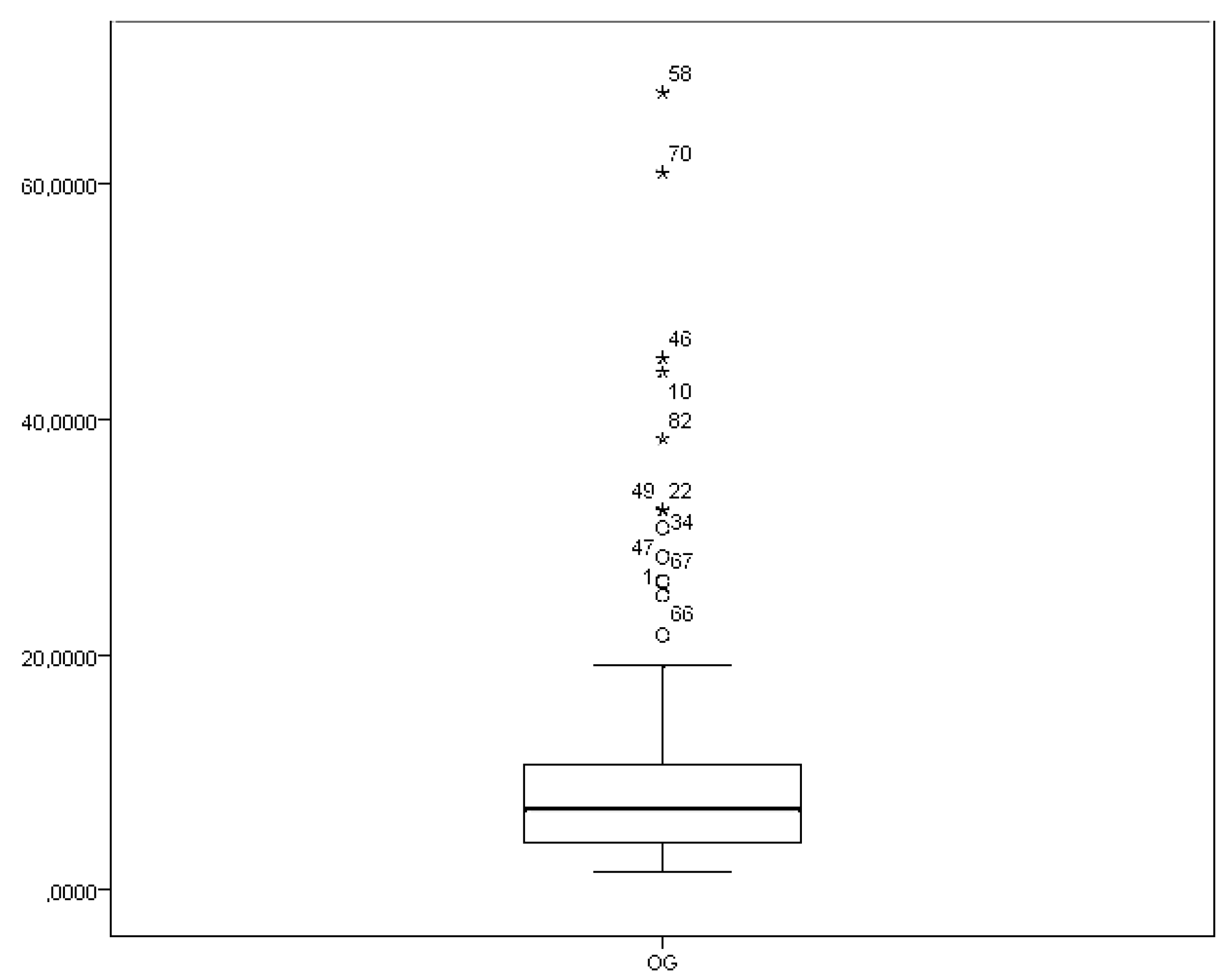
The box-plot of the classic MD is given in Figure 1. Here the classic MD is defined in Definition 2.
The source of the outliers is vague when we treat the data as a whole. Figure 1 shows that the most extreme individuals are the 58th, 70th and 46th, etc. As discussed before, information about the source of the outliers is unavailable since the structure of the model is not separated.
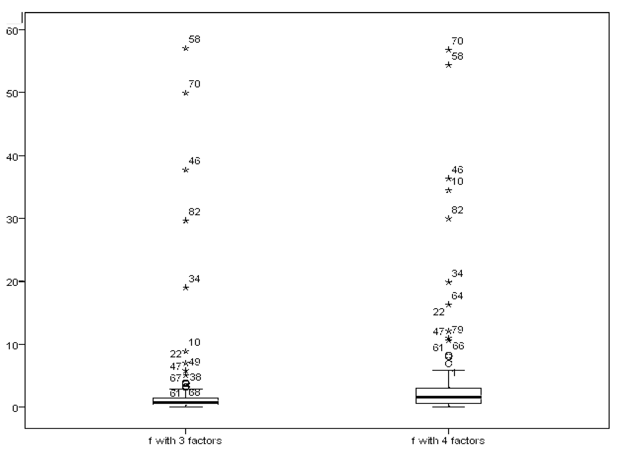
Next, we turn to the separated MDs to get more information. We show the box–plots of the separate parts in the factor model in Figure 2 and Figure 3.
In our case, we choose the number of factors as 3 and 4 based on economic theory and the supportive results from scree plots. In the factor model, we use the maximum likelihood method to estimate the factor loadings. For the factor scores, we use the weighted least square method which is also known as “Bartlett’s method”. Readers are referred to the literature for details of the methods (Anderson 2003; Johnson and Wichern 2002).
Compared with Figure 1, we get different orders of the outliers. For the factor score part, the most distinct outliers are the 58th, 70th and 46th. Figure 2 shows that, from the error part, the most distinct outliers are the 82nd, 58th and 34th, while the first three outliers in the classic MD are the 58th, 70th and 46th. By using this method, we distinguish the outliers from different parts of the factor model. It helps us to detect the source of outliers. In addition to the figures, we also implemented our model in other factor structures with different numbers of factors (5 and 6 factors). The results showed a similar pattern. The maximum stock returning rates are the same as the ones we found from the factor structure model with 3 or 4 factors. The reliability of the factor analysis on this data set has also been investigated and confirmed.
6. Conclusions and Discussion
We investigate a new solution on detecting outliers based on the information from internal structure of data sets. By using a factor model, we reduce the dimension of the data set to improve the estimation efficiency of the covariance matrix. Further, we detect outliers based on a separated factor model that consisted by the error part and the systematic part. The new way of detecting the outliers is investigated by an empirical application. The results show that different source of outliers is detectable and can imply a different view inside the data.
We provide a different perspective on how to check the data set by investigating the source of outliers. In a sense, the new method helps us to improve the accuracy of inference since we can filter the observations more carefully based on different sources. The proposed method leads to different conclusions compared to the classic method.
We employed the sample covariance matrix as part of the estimated factor scores. The sample covariance matrix is not the optimal component since it is sensitive to the outlier. Thus, some further study can be conducted based on the results of this paper. In addition to the results above, further studies can be developed for non-normality distributed variables case especially when the sample size is relatively small. Because the violation of the multivariate normal distribution assumption will lead to severe results for example but not limited: model fit statistics (i.e., the fit statistic and statistics based on such as Root mean square error of approximation). The model fit statistics will further affect the specification of the factor model by misleading choosing the number of factors in the fitted model. Some assumptions such as above is imposed to simplify the work of derivation. This is such a strong imposition that it may not be valid in reality all the time. Thus, some further research could be conducted in this direction.
Acknowledgments
Thanks to the referees and the Academic Editor for their constructive suggestions to improve the presentation of this paper.
Conflicts of Interest
The author declares no conflict of interest.
Appendix A. Proof of Propositions
Proof of Proposition 2.
The sample covariance matrix for the estimated factor loadings and covariance of error term is defined as According to Lawley and Maxwell (1971), we have , thus, □
Proof of Proposition 4.
Without loss of generality, we set . The factor scores based MD is . Since (Johnson and Wichern 2002), by using the results and where stands for convergence in probability (Anderson 2003), we get where . Set , we get the first moment as . Follow the same way, we get the variance of the factor scores based MD as .
Given the error terms are homogeneous, we get that where is a constant across the different factors. The proof for the error terms follows the same pattern as the factor score based MD. We skip it in the proof. □
Proof of Proposition 5.
By Proposition 5 (i):.
Set then,
Since the outlier is deterministic, it is independent of the factor scores and the error term . By using and , we get the convergence in probability with and so is the error term . Note that replacing with will not affect the asymptotic properties. Thus, . Hence, . Thus, for , we extend the expression as where . For , let , plug into the expression above and we get where these parts are equivalent to ,
, By all the results above, we extend the expression that
For Proposition 5 (ii), it follows directly from part (i). □
Linear invariance of factor models MD (covariance matrix): Let the linear transformation of data be where is the symmetric invertible matrix, then the new MD under the linear transformation is given as follows:
where (Mardia 1977). Using this connection, we get, . Thus, the MD for factor models is linear transform invariant.
The MLE of factor loadings: The maximum likelihood estimator for the mean vector , the factor loadings and the specific variances are obtained by finding , , and that maximises the log likelihood, which is given by the following expression:
The log of the joint probability distribution of the data is to be maximised.
References
- Anderson, Theodore Wilbur. 2003. An Introduction to Multivariate Statistical Analysis, 5th ed. Hoboken: Wiley. [Google Scholar]
- Bai, Jushan. 2003. Inferential theory for factor models of large dimensions. Econometrica 71: 135–71. [Google Scholar] [CrossRef]
- Chalmers, R. Philip, and David B. Flora. 2015. Faoutlier: An r package for detecting influential cases in exploratory and confirmatory factor analysis. Applied Psychological Measurement 39: 573. [Google Scholar] [CrossRef] [PubMed]
- Fisher, Ronald A. 1940. The precision of discriminant functions. Annals of Human Genetics 10: 422–29. [Google Scholar] [CrossRef] [Green Version]
- Flora, David B., Cathy LaBrish, and R. Philip Chalmers. 2012. Old and new ideas for data screening and assumption testing for exploratory and confirmatory factor analysis. Frontiers in Psychology 3: 55. [Google Scholar] [CrossRef] [PubMed] [Green Version]
- Gorman, N. T., I. McConnell, and P. J. Lachmann. 1981. Characterisation of the third component of canine and feline complement. Veterinary Immunology and Immunopathology 2: 309–20. [Google Scholar] [CrossRef]
- Gregory, Allan W., and Allen C. Head. 1999. Common and country-specific fluctuations in productivity, investment, and the current account. Journal of Monetary Economics 44: 423–51. [Google Scholar] [CrossRef] [Green Version]
- Harville, David A. 1997. Matrix Algebra from a Statistician’s Perspective. New York: Springer. [Google Scholar]
- Holgersson, H. E. T., and Ghazi Shukur. 2001. Some aspects of non-normality tests in systems of regression equations. Communications in Statistics-Simulation and Computation 30: 291–310. [Google Scholar] [CrossRef]
- Johnson, Richard Arnold, and Dean W. Wichern. 2002. Applied Multivariate Statistical Analysis, 5th ed. Upper Saddle River: Prentice Hall. [Google Scholar]
- Lawley, Derrick Norman, and Albert Ernest Maxwell. 1971. Factor Analysis as a Statistical Method. London: Butterworths. [Google Scholar]
- Lewbel, Arthur. 1991. The rank of demand systems: theory and nonparametric estimation. Econometrica 59: 711–30. [Google Scholar] [CrossRef]
- Mahalanobis, Prasanta Chandra. 1936. On the Generalized Distance in Statistics. Odisha: National Institute of Science of India, vol. 2, pp. 49–55. [Google Scholar]
- Mardia, Kanti V. 1974. Applications of some measures of multivariate skewness and kurtosis in testing normality and robustness studies. Sankhyā: The Indian Journal of Statistics, Series B 36: 115–28. [Google Scholar]
- Mardia, K. V. 1977. Mahalanobis distances and angles. Multivariate analysis IV 4: 495–511. [Google Scholar]
- Mardia, K. V., J. T. Kent, and J. M. Bibby. 1980. Multivariate Analysis. San Diego: Academic Press. [Google Scholar]
- Mavridis, Dimitris, and Irini Moustaki. 2008. Detecting outliers in factor analysis using the forward search algorithm. Multivariate Behavioral Research 43: 453–75. [Google Scholar] [CrossRef] [PubMed]
- Pavlenko, Tatjana. 2003. On feature selection, curse-of-dimensionality and error probability in discriminant analysis. Journal of Statistical Planning and Inference 115: 565–84. [Google Scholar] [CrossRef]
- Pek, Jolynn, and Robert C. MacCallum. 2011. Sensitivity analysis in structural equation models: Cases and their influence. Multivariate Behavioral Research 46: 202–28. [Google Scholar] [CrossRef] [PubMed]
- Pison, Greet, Peter J. Rousseeuw, Peter Filzmoser, and Christophe Croux. 2003. Robust factor analysis. Journal of Multivariate Analysis 84: 145–72. [Google Scholar] [CrossRef] [Green Version]
- Rao, C. Radhakrishna. 2009. Linear Statistical Inference and its Applications. New York: John Wiley & Sons, vol 22. [Google Scholar]
- Ross, Stephen A. 1976. The arbitrage theory of capital asset pricing. Journal of Economic Theory 13: 341–60. [Google Scholar] [CrossRef]
- Styan, George P. H. 1970. Notes on the distribution of quadratic forms in singular normal variables. Biometrika 57: 567–72. [Google Scholar] [CrossRef]
- Wilks, Samuel S. 1963. Multivariate statistical outliers. Sankhyā: The Indian Journal of Statistics, Series A 25: 407–26. [Google Scholar]
- Yuan, Ke-Hai, and Xiaoling Zhong. 2008. 8. outliers, leverage observations, and influential cases in factor analysis: Using robust procedures to minimize their effect. Sociological Methodology 38: 329–68. [Google Scholar] [CrossRef]
Figure 1.
The box–plot of for the stock data.

Figure 2.
The box–plot of .
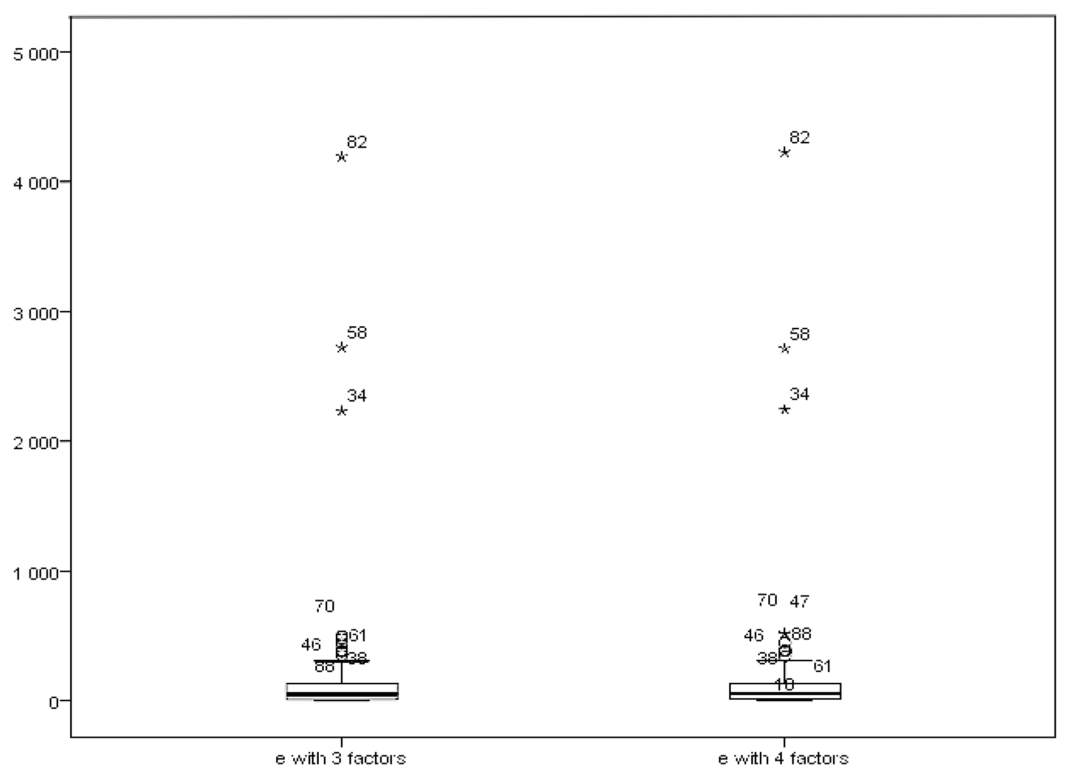
Figure 3.
The box–plot of .
© 2020 by the author. Licensee MDPI, Basel, Switzerland. This article is an open access article distributed under the terms and conditions of the Creative Commons Attribution (CC BY) license (http://creativecommons.org/licenses/by/4.0/).
Share and Cite
MDPI and ACS Style
Dai, D. Mahalanobis Distances on Factor Model Based Estimation. Econometrics 2020, 8, 10. https://0-doi-org.brum.beds.ac.uk/10.3390/econometrics8010010
AMA Style
Dai D. Mahalanobis Distances on Factor Model Based Estimation. Econometrics. 2020; 8(1):10. https://0-doi-org.brum.beds.ac.uk/10.3390/econometrics8010010
Chicago/Turabian StyleDai, Deliang. 2020. "Mahalanobis Distances on Factor Model Based Estimation" Econometrics 8, no. 1: 10. https://0-doi-org.brum.beds.ac.uk/10.3390/econometrics8010010
Note that from the first issue of 2016, this journal uses article numbers instead of page numbers. See further details here.