A Review of the ‘BMS’ Package for R with Focus on Jointness

Abstract

We provide a general overview of Bayesian model averaging (BMA) along with the concept of jointness. We then describe the relative merits and attractiveness of the newest BMA software package, BMS, available in the statistical language R to implement a BMA exercise. BMS provides the user a wide range of customizable priors for conducting a BMA exercise, provides ample graphs to visualize results, and offers several alternative model search mechanisms. We also provide an application of the BMS package to equity premia and describe a simple function that can easily ascertain jointness measures of covariates and integrates with the BMS package.

1. Introduction

Interest in Bayesian analysis, generally, and Bayesian model averaging (BMA), specifically, has increased rapidly as computational power of desktops and personal laptops have expanded (Steel 2019). With the demand for these tools comes an array of platforms with which to implement them. One of the most popular statistical softwares for any type of Bayesian analysis is the open source statistical environment R (R Development Core Team 2013). Even with the ability to conduct Bayesian analysis in R, there exist a wide variety of packages and compiled code; a user interested in BMA or variable selection has at their fingertips over 13 packages that can do the job (Forte et al. 2018). Given such a large menu of options, the uninitiated may not know which direction to go to start their analysis. A useful starting point is the BMS package.1

The BMS package (Feldkircher and Zeugner 2009; Zeugner and Feldkircher 2015) implements linear BMA with a comprehensive choice of priors, Monte Carlo Markov Chain samplers, and post-processing functions. This package provides a large degree of flexibility in the specification of the underlying features used to analyze the model and produces a wide range of easily-readable outputs including the posterior inclusion probabilities, means, and standard deviations, the number of models visited, and the number of draws from the sample. This package also takes advantage of R’s powerful graphical interface and creates useful graphs that allow the user to visualize the posterior model size distribution, posterior model probabilities, and cumulative model probabilities as well as providing plotting facilities for the marginal densities of the posterior coefficients.

Aside from the standard objects of interest in a BMA exercise (such as posterior inclusion probabilities, the highest probability model, etc.), attention has also been focused on jointness (Doppelhofer and Weeks 2009). Jointness captures dependence between covariates across the model space for the posterior distribution. Rather than focus on an individual variable’s inclusion, jointness quantifies how likely two variables are to appear together. In the presence of model uncertainty, this joint inclusion can be important across a variety of dimensions (Man 2018). However, jointness can take many different forms (Doppelhofer and Weeks 2009; Ley and Steel 2009b; Strachan 2009) and many of the measures that have been proposed have limitations in one form or another, depending on the range of properties considered for a measure of jointness (Hofmarcher et al. 2018). As yet, a consensus does not exist as to the best measure of jointness, nor is it well understood how robust a given jointness measure is across various user defined choices (such as choice of prior), though Man (2018) is one step in this direction.

This paper details both the basic functionality of the BMS package and provides an easy to deploy function that calculates eight different jointness measures. We begin with an overview of both BMA and jointness. We then detail how to install the BMS package and implement a BMA empirical exercise using this package. We describe the main features under the user’s control for this package including the set of prior probabilities and model sampling algorithms as well as the plot diagnostics available to visualize the results. We show how a user can obtain estimates, posterior inclusion probabilities, and model statistics from this package with a mock empirical example. We do this both with a set of covariates that allows for full enumeration of the model space as well as requiring the implementation of a model space search mechanism. Lastly, we follow up with an application to the equity premium from the finance literature and provide an R routine that users can implement within BMS to calculate jointness across eight different measures. Having access to these various measures allows users to quickly determine how robust alternative findings of jointness are to various changes in the setup of the BMA exercise.

2. Bayesian Model Averaging

In brief, the implementation of BMA begins by considering a set of possible models, say $M=\{M_1,M_2,\dots ,M_K\}$. M represents the model space the averaging will be conducted over. Once this space has been set the posterior distribution of any quantity of interest, $\theta$, given the data, D, is

$$Pr\left(\theta \right|D)=\sum _{j=1}^{K}Pr\left(\theta \right|M_j,D)Pr\left(M_j\right|D),$$

(1)

which is simply the weighted average of the posterior distributions under each model.

The most common framework for BMA is the linear regression model of the form

$$y|\alpha ,{\beta }_j,\sigma \sim N(\alpha +X_j{\beta }_j,{\sigma }^{2}I),$$

(2)

where y is the $n\times 1$ dependent variable vector and $X_j$ the $n\times {\ell }_j$ matrix of covariates. Here, there are potentially L covariates. In this case, $\theta =\{\alpha ,\beta ,{\sigma }^2\}$, where ${\beta }_j$ is a subvector or $\beta$.

Using Bayes Theorem, one can rewrite the posterior probability of model $M_k$ as follows:

$$\begin{array}{cc}\hfill & Pr\left(M_k\right|D)=Pr\left(D\right|M_k)\frac{Pr\left(M_k\right)}{Pr\left(D\right)}=Pr\left(D\right|M_k)\frac{Pr\left(M_k\right)}{\sum _{j=1}^{K}Pr\left(D\right|M_j)Pr\left(M_j\right)}\hfill \end{array}$$

(3)

$$\begin{array}{c}Pr\left(D\right|M_k)=\int Pr\left(D\right|{\theta }_k,M_k)Pr\left({\theta }_k\right|M_k)d{\theta }_k\hfill \end{array}$$

(4)

where ${\theta }_k$ is the vector of parameters from model $M_k$, $Pr\left({\theta }_k\right|M_k)$ is a prior probability distribution assigned to the parameters of model $M_k$, and $Pr\left(M_k\right)$ is the prior probability that $M_k$ is the true model. As mentioned above, in order to make BMA applicable, we need to choose prior distributions for the parameters of the model and then, based on the data, calculate posterior probabilities attached to different models and finally find the parameter distributions by averaging posterior distributions.

One should notice that, as stated in Brock et al. (2003, p. 270), ideally the set of prior probabilities should be informative with respect to the likelihood, meaning priors should assign relatively high probability to areas that have high likelihood. Were this not the case then the choice of priors will have a substantial effect on the posteriors. Unfortunately, the likelihood is unknown, making the choice of the prior user specific. Several studies have attempted to discern the effect that the choice of prior probabilities has on posterior probabilities, which are commonly used to gauge the ‘robustness’ of a variable. This is not to be confused with variable importance, which attempts to discern if a variable belongs to the true model.2 Rather, robustness seeks to determine how small changes to the prior probability structure impact the posterior estimates. Ley and Steel (2009a) and Steel (2019) provide a complete review on the effect of prior assumptions on the outcome of BMA analyses. As will be important later when we discuss the BMS package, the ability of a software package to allow the user to vary the prior to assess small changes is important to allow researchers the ability to gauge robustness.

The issues with BMA highlighted here are by no means an indictment of the methods. Rather, they are to draw attention to the areas where the user must exert caution when implementing a model averaging exercise. Undoubtedly, for any model averaging investigation, the researcher will face issues based on the route taken to average across models. Furthermore, understanding the nuances of model averaging exercises allows for clearer comparisons and the ability to understand where results may differ. We counsel interested readers to consult Moral-Benito (2015), Fletcher (2018), or Steel (2019) for a review of the state of the art.

3. Jointness

Capturing the dependence between explanatory variables in the posterior distribution while implementing a Bayesian analysis is crucial. Taking such a dependence into account reveals the sensitivity of posterior distributions of parameters to dependence across regressors. For instance, if two specific variables are complementary over the model space, we expect relatively higher weights for the models that include both variables together than models where only one variable is present.

In this section, we discuss how the applied literature has focused on quantifying the dependence between predictive variables. The methodology behind BMA provides a measure for the marginal posterior inclusion probability of a given regressor. However, although the marginal probability measure of variable importance has interesting policy implications and prediction, it hardly provides information on the nature of dependencies among regressors. To address this issue, we follow Doppelhofer and Weeks (2009) and Ley and Steel (2009b) and introduce the posterior joint inclusion probability of variables $x_h$ and $x_l$ as

$$J_{hl}^{Pure}=p(x_h\cap x_l|D)=\sum _{i:x_h\&x_l\in M_i}Pr\left(M_i\right|D)$$

(5)

where $M_i$ is the ith model, and D is the data. This equation adds up posterior model probabilities for all the models in which the two variables are present. These posterior model probabilities are calculated as the weighted sum of the prior model probability times its marginal likelihood:

$$Pr\left(M_i\right|D)=\frac{{\ell }_D\left(M_j\right)Pr\left(M_j\right)}{{\displaystyle \sum _{k=1}^K}{\ell }_D\left(M_k\right)Pr\left(M_k\right)},$$

(6)

with the marginal likelihood defined as

$${\ell }_D\left(M_j\right)=\int p\left(D\right|{\theta }_j,M_j)p\left({\theta }_j\right|D,M_j).$$

For the linear regression model with normal priors on $\alpha$ and $\beta$, coupled with a gamma prior for ${\sigma }^2$, it can be shown (Steel 2019, p. 22) that the marginal likelihood is ${\ell }_D\left(M_j\right)\propto {(1+g)}^{(n-1-K_j)/2}{(1+g(1-R_j^2))}^{-(n-1)/2}$, where g comes from the g-prior of Zellner (1986), and $K_j$ is the number of covariates in model j where $R_j^2$ is the traditional in-sample measure of fit. Posterior model probabilities also form the basis for the calculation of posterior inclusion probabilities, which is simply the sum of the posterior model probabilities that contain a specific covariate.

From this discussion, a natural measure of dependence between variables $x_h$ and $x_l$ is given by3

$$J_{hl}^{DW1}=ln\left[\frac{p(x_h\cap x_l|D)}{p({\overline{x}}_h\cap x_l|D)·p(x_h\cap {\overline{x}}_l|D)}\right].$$

(7)

An alternative measure provided by Doppelhofer and Weeks (2009) is

$$J_{hl}^{DW2}=ln\left[\frac{p(x_h\cap x_l|D)·p({\overline{x}}_h\cap {\overline{x}}_l|D)}{p({\overline{x}}_h\cap x_l|D)·p(x_h\cap {\overline{x}}_l|D)}\right].$$

(8)

Ley and Steel (2009b) modify the jointness statistics of Doppelhofer and Weeks (2009) proposing the following two measures of jointness:

$$\begin{array}{cc}\hfill J_{hl}^{LS1}& =\frac{p(x_h\cap x_l|D)}{p(x_h\cup x_l|D)}\hfill \end{array}$$

(9)

$$\begin{array}{cc}\hfill J_{hl}^{LS2}& =\frac{p(x_h\cap x_l|D)}{p({\overline{x}}_h\cap x_l|D)+p(x_h\cap {\overline{x}}_l|D)}.\hfill \end{array}$$

(10)

Additionally, Strachan (2009) proposed

$$J_{hl}^{St}=p\left(x_h\right|D)p\left(x_l\right|D)ln\left[\frac{p(x_h\cap x_l|D)}{p({\overline{x}}_h\cap x_l|D)·p(x_h\cap {\overline{x}}_l|D)}\right].$$

(11)

Finally, in a detailed treatment of jointness, Hofmarcher et al. (2018) proposed two alternative measures:

$$J_{hl}^{YQ}=\frac{p(x_h\cap x_l|D)p({\overline{x}}_h\cap {\overline{x}}_l|D)-p({\overline{x}}_h\cap x_l|D)p(x_h\cap {\overline{x}}_l|D)}{p(x_h\cap x_l|D)p({\overline{x}}_h\cap {\overline{x}}_l|D)+p({\overline{x}}_h\cap x_l|D)p(x_h\cap {\overline{x}}_l|D)}$$

(12)

and

$$J_{hl}^{YQM}=\frac{\left(p(x_h\cap x_l|D)+0.5\right)\left(p({\overline{x}}_h\cap {\overline{x}}_l|D)+0.5\right)-\left(p({\overline{x}}_h\cap x_l|D)+0.5\right)\left(p(x_h\cap {\overline{x}}_l|D)+0.5\right)}{\left(p(x_h\cap x_l|D)+0.5\right)\left(p({\overline{x}}_h\cap {\overline{x}}_l|D)+0.5\right)+\left(p({\overline{x}}_h\cap x_l|D)+0.5\right)\left(p(x_h\cap {\overline{x}}_l|D)+0.5\right)-0.5}.$$

(13)

They show these two statistics have formal statistical and intuitive meaning in terms of jointness, and are more likely to be well-behaved when the posterior inclusion probability of one of the regressors is either zero or very close to zero.4 An interesting feature of $J_{hl}^{YQ}$ is that it maps the jointness measure of Doppelhofer and Weeks (2009), Equation (8), from $(-\infty ,\infty )$ to $[-1,1]$.

Given these various proposals to measure jointness, a natural question to ask is which one should be used for applied work. Hofmarcher et al. (2018) lists seven key properties that jointness measures, in general, may possess

• Definition: is the jointness measure defined whenever the one of the variables in included with positive probability (this is criteria C4 in Ley and Steel (2007));
• Monotonicity/Boundedness/Maximality: is the range of association between $x_l$ and $x_h$ bounded; is the measure monotonically increasing between the boundaries; the jointness measure only achieves the boundaries if both variables either always or never appear together (maximality is criteria C3 in Ley and Steel (2007));
• Limiting Behavior: The jointness measure should converge to its maximal value as the probability that $x_l$ and $x_h$ appear together increases to 1 and should converge to its minimal value as the probability that $x_l$ and $x_h$ appear separately increases to 1;
• Bayesian Confirmation: the jointness measure equals 0 if and only if the inclusion of $x_l$ and $x_h$ are statistically independent events;
• Non Null-Invariance: the jointness measure should not ignore model specifications where $x_l$ and $x_h$ and jointly excluded;
• Commutative Symmetry: suitable measures of jointness statistics should be symmetric to the ordering of variables;
• Hypothesis Symmetry: if $x_l$ and $x_h$ are complements for a given jointness measure, then ${\overline{x}}_l$ and $x_h$ are substitutes (disjoint) by the same jointness measure.

Only the modified Yule’s Q measure of jointness, Equation (13), satisfies all seven of these properties, whereas every jointness statistic presented here satisfies commutative symmetry. Ley and Steel (2007) also argue that any jointness measure should have a formal statistical meaning (what they term Interpretability), and the values that the jointness measure can take on should be calibrated against a clearly defined scale (what they term Calibration).

Positive (or large) values for jointness statistics indicate that variables $x_h$ and $x_l$ are complements, reflecting that posterior probabilities of models jointly including and excluding both variables are larger than posterior probabilities of models including only one. A negative (or small) value for the statistic, on the other hand, indicates that the variables are capturing a similar underlying effect and are disjoint; as noted in Steel (2019, p. 43), disjoint variables suggest that these variables are more likely to appear in a model separately from one another. Disjointness can arise when a pair of covariates are highly collinear or may be thought of as proxies/substitutes for each other. Note that, for $J^{LS1}$ and $J^{LS2}$, the lower bound for jointness is 0. It is common in practice to take the logarithm of these measures, see Ley and Steel (2009a).

The magnitude of the jointness statistics of Doppelhofer and Weeks (2009) is sensitive to whether or not the posterior inclusion probability of one of the explanatory variables is zero or extremely small, a case that commonly occurs in practice. As noted in Hofmarcher et al. (2018), a key property of any jointness measure is that it should be ‘defined’ whenever one of the variables is included with positive probability. This property is fulfilled by the two alternative measures proposed by Ley and Steel (2009b) as well as those introduced by Hofmarcher et al. (2018) but not by the measures proposed in Doppelhofer and Weeks (2009) or Strachan (2009). R code to construct all of the jointness measures discussed here is provided in Appendix A.

4. The BMS Package

Having now discussed both BMA and notions of jointness, we turn to how users can conduct a BMA exercise and calculate different jointness scores. Our platform for this is the BMS package.

4.1. Installation and Install Setup

Prior to invocation of the BMS package, R must be installed. R can be downloaded at no charge from http://www.cran.r-project.org. The R statistical environment runs on all common operating systems including Linux, Unix, Windows, and Mac-OS X.5 Once R is installed, it is preferable to install BMS directly within R simply by typing

in your R console. Then, you will be prompted to choose a CRAN repository and the package should be installed after a few seconds. The package can then be loaded into the R workspace by typing library (BMS) at the command prompt.6 For users who prefer to work with MATLAB, the core functionality of the BMS package can be accessed via the BMS Toolbox for Matlab. This toolbox provides MATLAB core functions that perform BMA by calling a hidden instance of R. This functionality requires a Windows operating system (NT, XP, Vista, 7, or 8) and the installation of both MATLAB (Version 6 or higher) and the R statistical environment.7

4.2. Functionality

The main command within the BMS package is bms() which deploys a standard Bayesian normal-conjugate linear model (see Equation (2)). Primarily, the options for the bms() command hinge on sampling from the model space and selection of both model priors and Zellner’s g-priors. These three categories comprise the most important aspects of conducting a BMA exercise.

4.3. Controlling the BMA Exercise

4.3.1. Model Sampling

A BMA analysis begins with constructing model weights for each model within the defined model space. However, since enumerating all potential variable combinations quickly becomes infeasible for even a modest number of covariates, the BMS package uses a Markov Chain Monte Carlo (MCMC) samplers to gather results on the most important part of the posterior distribution when more than 14 covariates exist.

The BMS package offers two different MCMC samplers to probe the model space. These two methods differ in the way they propose candidate models. The first method is called the birth-death sampler (mcmc=bd). In this case, one of the potential regressors is randomly chosen; if the chosen variable is already in the current model $M_i$, then the candidate model $M_j$ will have the same set of covariates as $M_i$ but drops the chosen variable. If the chosen covariate is not contained in $M_i$, then the candidate model will contain all the variables from $M_i$ plus the chosen covariate; hence, the appearance (birth) or disappearance (death) of the chosen variable depends if it already appears in the model. The second approach is called the reversible-jump sampler (mcmc=rev.jump). This sampler draws a candidate model by the birth-death method with 50% probability and with 50% probability the candidate model randomly drops one covariate with respect to $M_i$ and randomly adds one random variable from the potential covariates that were not included in model $M_i$.

The precision of any MCMC sampling mechanism depends on the number of draws the procedure runs through. Given that the MCMC algorithms used in the BMS package may begin using models which might not necessarily be classified as ‘good’ models, the first set of iterations do not usually draw models with high posterior model probabilities (PMP). This indicates that the sampler will only converge to spheres of models with the largest marginal likelihoods after some initial set of draws (known as the burn-in) from the candidate space. Therefore, this first set of iterations will be omitted from the computation of future results. In the BMS package, the argument (burn) specifies the number of burn-ins (models omitted), and the argument (iter) the number of subsequent iterations to be retained. The default number of burn-in draws for either MCMC sampler is 1000 and the default number of iteration draws to be sampled (excluding burn-ins) is 3000 draws.

4.3.2. Model Priors

The BMS package offers considerable freedom in the choice of model prior. One can employ the uniform model prior as the choice of prior model size (mprior=“uniform”), the Binomial model priors8 where the prior probability of a model is the product of inclusion and exclusion probabilities (mprior=“fixed”), the Beta-Binomial model prior (mprior=“random”) that puts a hyperprior on the inclusion probabilities drawn from a Beta distribution9 or a custom model size and prior inclusion probabilities (mprior=“customk”).

4.3.3. Alternative Zellner’s g-Priors

Different mechanisms have been proposed in the literature for specifying g priors. The options in the BMS package are as follows:

• g="UIP"; Unit Information Prior that corresponds to $g=N$, the sample size (see Fernández et al. 2001).
• g="RIC"; Sets $g=K^2$ and conforms to the risk inflation criterion (see Foster and George 1994, for more details).
• g="BRIC"; A mechanism that asymptotically converges to the unit information prior ($g=N$) or the risk inflation criterion ($g=K^2$). That is, the g prior is set to $g=max(N,K^2)$ (see Fernández et al. 2001).
• g="HQ"; Follows the Hannan–Quinn criterion asymptotically and sets $g=log\left(N^3\right)$.
• g="EBL"; Estimates a local empirical Bayes g-parameter (see Foster and George 2000; Liang et al. 2008).
• g="hyper"; Takes the “hyper-g” prior distribution (see Feldkircher and Zeugner 2009; Liang et al. 2008).

4.4. Outputs

In addition to posterior inclusion probabilities (PIP) and posterior means and standard deviations, bms() returns a list of aggregate statistics including the number of draws, burn-ins, models visited, the top models, and the size of the model space. It also returns the correlation between iteration counts and analytical PMPs for the best models, those with the highest PMPs.

4.5. Plot Diagnostics

BMS package users have access to plots of the prior and posterior model size distributions, a plot of posterior model probabilities based on the corresponding marginal likelihoods and MCMC frequencies for the best models that visualize how well the sampler has converged. A grid with signs and inclusion of coefficients vs. posterior model probabilities for the best models and plots of predictive densities for conditional forecasts are also produced.

4.6. Empirical Illustration

This section shows the results of a basic BMA exercise using the Hedonic dataset available in the plm package Croissant and Millo (2008). This dataset contains information aggregated across census tracts for the Boston metropolitan area in 1970, originally published in Harrison and Rubinfeld (1978). This cross-sectional dataset consists of 506 observations along with 13 potential determinants of median housing prices in Boston. The dependent variable ($MV$) is the corrected median value of owner-occupied homes in $1000s, and among the explanatory variables are the per capita crime rate ($CRIM$), the pupil–teacher ratio by town school district ($PTRATIO$), the index of accessibility to radial highways ($RAD$), the proportion of owner-occupied units built prior to 1940 ($AGE$), the proportion of non-retail business acres per town ($INDUS$), the proportion of African-Americans per town (B), and a variable reflecting the nitric oxides concentration ($NOX$). See Harrison and Rubinfeld (1978, Table 4) for more details.

The authors use a hedonic housing price model to generate quantitative estimates of the willingness to pay for air quality improvements. We assume there exists uncertainty about which housing attributes should be a part of the true model. The small number of covariates allows the bms() command to fully enumerate the model space, i.e., every possible model in M is estimated prior to averaging. To further demonstrate searching over the model space, we append 12 fictitious variables, generated as independent standard normal random deviates, which pushes the number of covariates beyond the threshold search level and requires MCMC methods. These 12 additional variables have no impact on median housing prices and are introduced here only to demonstrate how well the BMS package works when there are a large number of covariates. We present diagnostic plots to illustrate the flexibility of the calls within the package.

4.6.1. Enumeration of the Model Space

We first present the results of performing basic BMA with the original Hedonic dataset, which is small enough to fully enumerate the model space. First, we load the required packages and set the R options via the following commands:

Next, we load the dataset, append the 12 fictitious variables, and manipulate it using the following commands:

Now, we perform BMA via the bms() command, and retrieve the main results via the coef function. The following commands will implement the BMA analysis over the Hedonic dataset.

In this setup, bms() enumerates all $2^{13}=8192$ models. The current call uses a uniform distribution for model priors and unit information priors (UIP) for the distribution of regressions coefficients.

Table 1. Bayesian Model Averaging Estimates. The first column, named PIP, shows the posterior inclusion probabilities indicating the probability that each variable belongs to the true model. BMS sorts these probabilities from the highest to the lowest automatically. The second and third columns show the posterior means and standard errors of regressors calculated from this package.

Variable	PIP	Post Mean	Post Std
Crime Rate	1.00	−0.012	0.001
Lower-Status Population	1.00	−0.371	0.023
Distance to Employment Center	1.00	−0.194	0.027
Pupil-Teacher Ratio	1.00	−0.031	0.005
Nitrogen Oxide Concentration	1.00	−0.006	0.001
Number of Rooms	1.00	0.006	0.001
Access to Radial Highways	1.00	0.095	0.019
Property Tax Rate	0.99	−0.000	0.000
Black People Percentage	0.96	0.355	0.122
Charles River Dummy	0.70	0.064	0.050
Non-Retail Business Acres	0.04	0.000	0.001
Owner Units Built Prior to 1940	0.04	0.000	0.000
Proportion of 25,000 Square Feet Residential Lots	0.04	0.000	0.000

shows the output for model.enu.

The first column, named PIP, shows the posterior inclusion probabilities indicating the probability that each variable belongs to the true model. BMS sorts these probabilities from the highest to the lowest automatically. The second and third columns show the posterior means and standard errors of regressors calculated from this package. Several key takeaways emerge from Table 1. Of the 13 variables in consideration, seven have PIPs of 1 and two more (Property Tax Rate and Black People Percentage) have PIPs above 0.95. Only three variables have PIPs low enough to suggest they do not belong to the true model. The magnitudes of the posterior means are also aligned with intuition.

Other additional information about the model averaging procedure can be obtained using the summary function. In our case, the output would be

As is apparent, some useful statistics including the number of models visited, the average number of regressors used, and time performance are produced.

4.6.2. Model Sampling

In this section, we present results obtained when full enumeration is computationally infeasible or undesirable. Using the Hedonic.large dataset, the following commands will implement the BMA analysis using the birth-death MCMC search algorithm (see Section 4.3.1) with 10,000 iterations and a burn in of 2000 models.

The PIPs for this exercise are shown in the first column of

Table 2. Bayesian Model Averaging Estimates. The first column, named PIP, shows the posterior inclusion probabilities indicating the probability that each variable belongs to the true model. BMS sorts these probabilities from the highest to the lowest automatically. The second and third columns show the posterior means and standard errors of regressors calculated from this package.

Variable	PIP	Post Mean	Post Std
Crime Rate	1.00	−0.012	0.001
Nitrogen Oxide Concentration	1.00	−0.006	0.001
Number of Rooms	1.00	0.006	0.001
Distance to Employment Center	1.00	−0.194	0.027
Access to Radial Highways	1.00	0.095	0.019
Pupil-Teacher Ratio	1.00	−0.031	0.005
Lower-Status Population	1.00	−0.371	0.023
Property Tax Rate	0.99	−0.000	0.000
Black People Percentage	0.97	0.353	0.119
Charles River Dummy	0.71	0.066	0.050

after invocation of the coef function on the BMS object. The choices for model priors and the distribution of the model coefficients are the uniform distribution and unit information priors, respectively. As in Table 1, the next two columns show the estimated posterior means and standard deviations of the covariates. Even with the addition of the 12 fictitious variables, the birth–death sampler provides PIPs consistent with the earlier full enumeration example. We do not list the PIPs for the 12 fictitious variables or the three variables with PIPs below 0.05 in Table 1. Even having to search the model space (which is orders of magnitude larger than with the original dataset), we see similar posterior mean and posterior standard deviation estimates across all covariates with the same signs.

Additional statistical information is revealed via the call

Note that the MCMC search algorithm visited less than one half of one percent of the total number of models in the model space and still provided results consistent with full enumeration over the model space.

4.6.3. Plot Diagnostics

The plotting facilities within BMS are an important tool that allows the user to visualize the shape of the posterior distributions of coefficients, assess the size of the true model, compare PIPs, and investigate model complexity. The BMS package plots the marginal inclusion densities as well as images that show inclusion and exclusion of variables within models using separate colors. This package also provides graphics for both the PMPs and posterior model size distribution. The following figures are some examples of the available plots corresponding to the above example where we added 12 fictitious covariates to force the package to engage in searching across the model space.

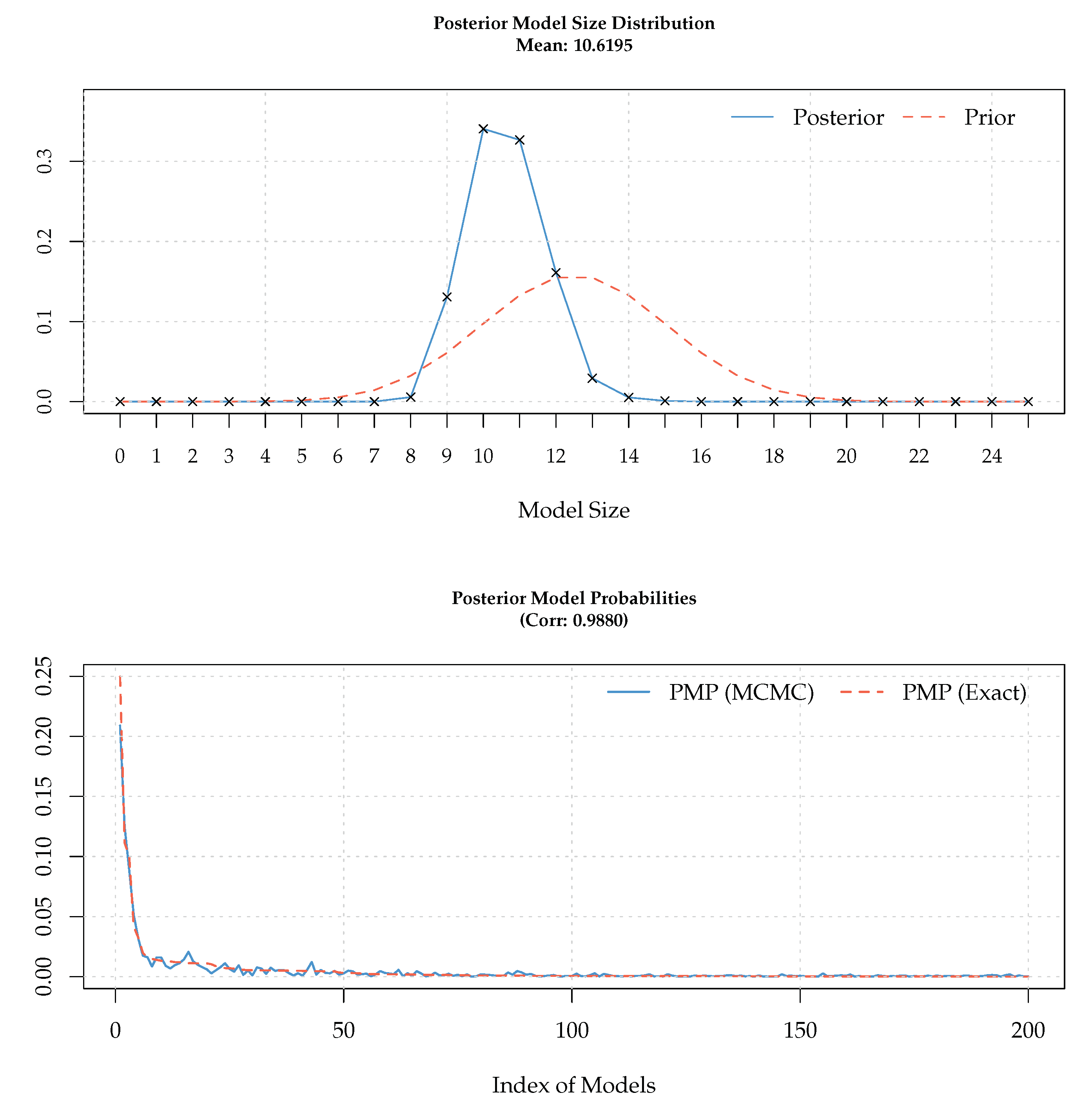
In order to produce a plot for comparison of prior and posterior distributions of the model size, simply use

The first argument in the command is the R object where we have saved our estimation results, and the second argument defines the type of line we are going to use for our graphs.

Figure 1 is a combined plot from the BMS package. The upper plot shows the prior and posterior distribution of model sizes and helps the user illustrate the impact of the model prior assumption on the estimation results. For example, the upper plot of Figure 1 assumes a uniform distribution on model priors and, if the user wants to examine how far the posterior model size distribution matches up to the prior, he might consider other popular model priors that allow more freedom in choosing prior expected model size and other factors. The lower plot of the figure is an indicator of how well the first 200 best models encountered by BMS have converged. These plots are useful in determining the search mechanisms ability to find ‘good’ models throughout the model space.

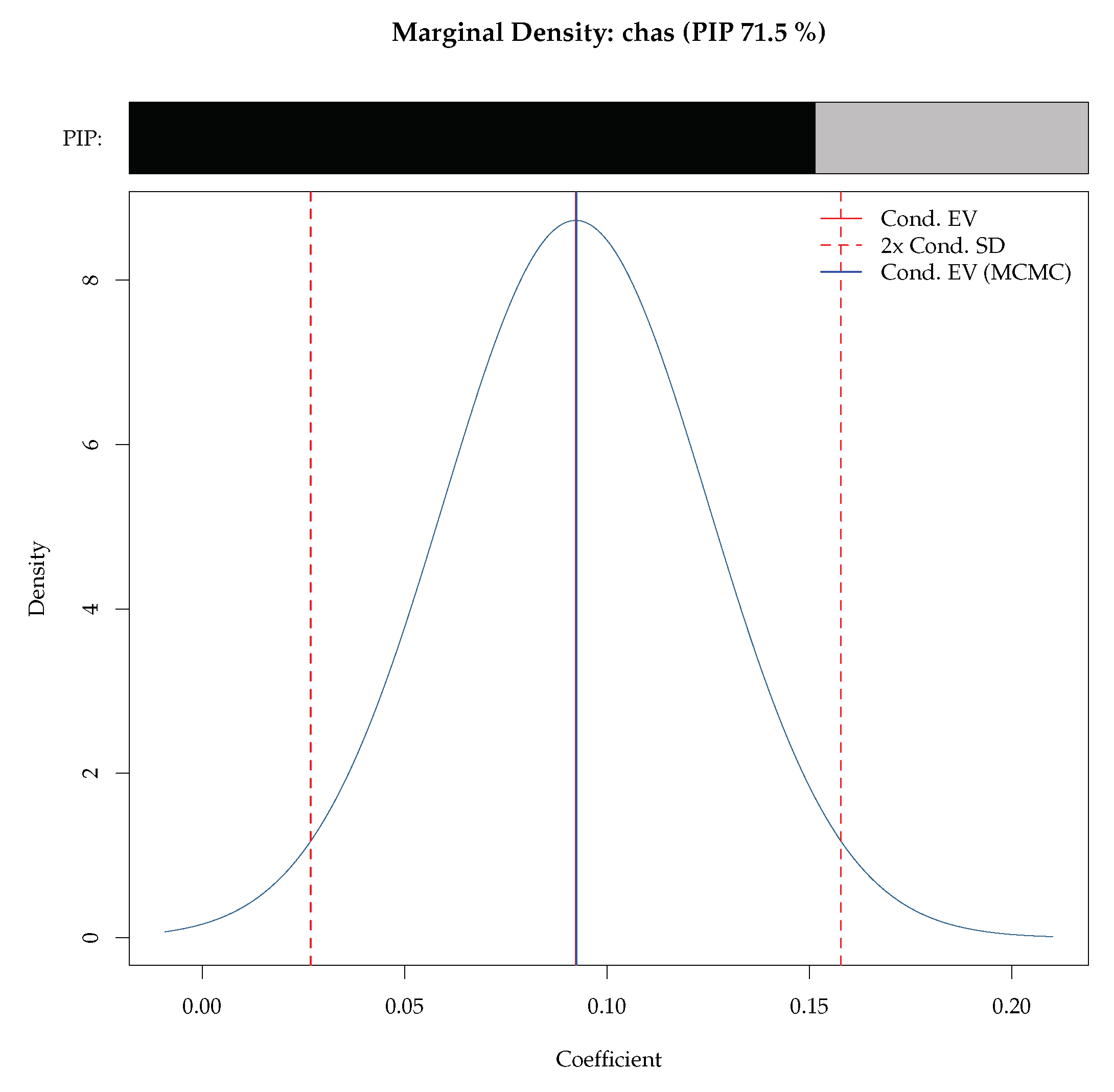
Figure 2 is a visualization of the mixture marginal posterior density for the coefficient for the Charles River Dummy produced by the BMS package. The bar above the density shows the PIP, and the dotted vertical lines show the corresponding standard deviation bounds. This figure can be generated simply via density.bma function within the BMS package

This is an extremely flexible command and provides several options for the user. Addons receives string values specifying which additional information should be added to the plot via low-level commands. To see more details, run help(density.bma) in your R console.

5. A Finance Application with Jointness

Financial economists have proposed numerous variables including dividend-price ratio, dividend yield, earnings-price ratio, dividend-payout ratio, stock variance, net equity issuance, treasury bill rate, return on long-term government bonds, term spread, book-to-market ratio, inflation, and investment-to-capital ratio, among others, along with different econometric techniques in attempts to predict the equity risk premium (Welch and Goyal 2008). However, a lack of consensus regarding theoretical frameworks has created situations where many possible models exist to explain the effect of a particular variable on equity premium. We argue that, under this circumstance, picking a single model tends to ignore the uncertainty associated with the specification of the selected model and may result in unstable outcomes. Hence, we suggest using BMA to combine all the competing models and compute a weighted average of the estimates to mitigate the uncertainty and instability risk associated with reliance on a single model. In this section, we deploy the BMS to identify the key determinants of equity premium.

The dataset used in this section is an extended version of the dataset described in Welch and Goyal (2008). Our sample period is from 1927 to 2013 and includes information on the following variables:

• Equity premium (eqp): Defined as the total rate of return on the stock market minus the prevailing short-term interest rate.
• Dividends: Dividend yield (dy) is the difference between the log of dividends and the log of lagged prices.
• Earnings: Earnings price ratio (e/p) is the difference between the log of earnings on the S&P 500 index and the log of prices. Dividend payout ratio (d/e) is the difference between the log of dividends and the log of earnings.
• Volatility: Stock variance (svar) is measured as the sum of squared daily returns on the S&P 500.
• Book value: Book-to-market ratio (b/m) is the ratio of book value at the end of the previous year divided by the end-of-month market value.
• Corporate issuing activity: Net equity expansion (nee) is the ratio of 12-month moving sums of net issues by NYSE listed stocks divided by the total end-of-year market capitalization of NYSE stocks.
• Treasury bills: T-bill rate (tbl) is the secondary market rate of three-month US treasury bills.
• Long-term yield: Long-term government bond yields (lty) and long-term government bond returns (ltr) are the yields and returns of long-term US treasury bonds, respectively.
• Corporate bond returns: Default return spread (dfr) is the difference between returns on long-term corporate bonds and returns on long-term government bonds. Default yield spread (dfy) is the difference between BAA-rated and AAA-rated corporate bond yields.
• Inflation: Inflation (infl) is the Consumer Price Index (all urban consumers) from the Bureau of Labor Statistics, lagged by one month.

Table 3. Summary Statistics for Equity Premium Sample. The table reports the summary statistics of the predictive variable proposed in the literature as potential determinants of equity premium in the US stock market. The sample include monthly observations from 1927 to 2013. Number of observations, mean, standard deviations, median, minimum, and maximum values for each variable are reported.

Variable	No. Observations	Mean	Std. Dev.	Min	Max	Median
Equity Premium (eqp)	1044	0.006	0.055	−0.288	0.414	0.009
Dividend Yield (d/y)	1044	−3.344	0.455	−4.531	−1.913	−3.312
Earnings Price Ratio (e/p)	1044	−2.722	0.419	−4.836	−1.775	−2.767
Dividend Payout Ratio (d/e)	1044	−0.627	0.333	−1.244	1.379	−0.617
Stock Variance (svar)	1044	0.003	0.006	0.000	0.071	0.001
Book-to-Market Ratio (b/m)	1044	0.580	0.266	0.121	2.028	0.558
Net Equity Expansion (nee)	1044	0.018	0.025	−0.058	0.176	0.019
Treasury Bill Rate (tbl)	1044	0.035	0.031	0.000	0.163	0.031
Long-Term Government Bond Yield (lty)	1044	0.052	0.028	0.018	0.148	0.043
Long-Term Government Bond Returns (ltr)	1044	0.005	0.024	−0.112	0.152	0.003
Default Return Spread (dfr)	1044	0.000	0.014	−0.098	0.074	0.001
Default Yield Spread (dfy)	1044	0.011	0.007	0.003	0.056	0.009
Inflation (infl)	1044	0.002	0.005	−0.021	0.057	0.002

presents summary statistics for the equity premium sample. The majority of the variables are nearly symmetric, with the earnings to price ratio and the dividend yield being slightly skewed. The long-term government bond yield has an average monthly return of 5.2%, but an average return of only 0.5%; this is also reflected in the minimum and maximum over the sample (−11.2–15.2%).

The posterior inclusion probabilities, posterior mean and standard deviation estimates of the coefficients are in

Table 4. Bayesian Model Averaging Estimates. The first column, PIP, shows the posterior inclusion probabilities indicating the probability that each variable belongs to the true model. BMS sorts these probabilities from the highest to the lowest automatically. The second and third columns show the posterior means and standard errors of regressors calculated from this package.

Variable	PIP	Post Mean	Post Std
Dividend Yield (d/y)	1.00	1.012	0.003
Earnings Price Ratio (e/p)	1.00	−1.009	0.003
Dividend Payout Ratio (d/e)	1.00	−1.010	0.003
Stock Variance (svar)	1.00	0.472	0.039
Treasury Bill Rate (tbl)	1.00	−0.089	0.007
Book-to-Market Ratio (b/m)	0.50	0.002	0.002
Default Yield Spread (dfy)	0.34	0.028	0.044
Default Return Spread (dfr)	0.08	0.001	0.006
Inflation (infl)	0.04	−0.000	0.002
Long-Term Government Bond Returns (ltr)	0.04	0.000	0.003
Net Equity Expansion (nee)	0.03	0.000	0.001
Long-Term Government Bond Yield (lty)	0.02	0.000	0.005

. Of the 12 variables, five have PIPs of one: dividend yield, earnings to price ratio, dividend payout ratio, stock variance and the treasury bill rate. The book-to-market ratio has a PIP of 0.5 which suggests some likelihood of inclusion in the true model, though its posterior mean is essentially 0. The remaining variables have low PIPs along with low posterior means and standard deviations. The magnitudes and signs of the five variables with PIPs of one are consistent with standard models of equity premia.

Turning our attention to jointness,

Table 5. Jointness. The table shows the level of dependency between any pair of regressors used to model equity premium using Doppelhofer and Weeks (2009).

	dy	epr	der	svar	bm	nee	tbl	lty	ltr	dfr	dfy	linfl
dy	.	–	–	–	–	–	–	–	–	–	–	–
epr	–	.	–	–	–	–	–	–	–	–	–	–
der	–	–	.	–	–	–	–	–	–	–	–	–
svar	–	–	–	.	–	–	–	–	–	–	–	–
bm	–	–	–	–	.	0.2	–	−0.5	−0.2	0.2	−2.1	−0.2
nee	–	–	–	–	0.2	.	–	−1.1	0.3	−0.4	0	0.3
tbl	–	–	–	–	–	–	.	–	–	–	–	–
lty	–	–	–	–	−0.5	−1.1	–	.	0.9	−0.2	−0.1	1.1
ltr	–	–	–	–	−0.2	0.3	–	0.9	.	−0.4	0	1.2
dfr	–	–	–	–	0.2	−0.4	–	−0.2	−0.4	.	0	0.6
dfy	–	–	–	–	−2.1	0	–	−0.1	0	0	.	0.5
linfl	–	–	–	–	−0.2	0.3	–	1.1	1.2	0.6	0.5	.

,

Table 6. Jointness. The table shows the level of dependency between any pair of regressors used to model equity premium using Ley and Steel (2009b) as presented in Equation (9).

	dy	epr	der	svar	bm	nee	tbl	lty	ltr	dfr	dfy	linfl
dy	.	Inf	Inf	Inf	1.2	0.1	Inf	0	0	0.1	0.4	0
epr	Inf	.	Inf	Inf	1.2	0.1	Inf	0	0	0.1	0.4	0
der	Inf	Inf	.	Inf	1.2	0.1	Inf	0	0	0.1	0.4	0
svar	Inf	Inf	Inf	.	1.2	0.1	Inf	0	0	0.1	0.4	0
bm	1.2	1.2	1.2	1.2	.	0.1	1.2	0	0	0.1	0.1	0
nee	0.1	0.1	0.1	0.1	0.1	.	0.1	0	0	0	0	0
tbl	Inf	Inf	Inf	Inf	1.2	0.1	.	0	0	0.1	0.4	0
lty	0	0	0	0	0	0	0	.	0	0	0	0
ltr	0	0	0	0	0	0	0	0	.	0	0	0
dfr	0.1	0.1	0.1	0.1	0.1	0	0.1	0	0	.	0.1	0
dfy	0.4	0.4	0.4	0.4	0.1	0	0.4	0	0	0.1	.	0
linfl	0	0	0	0	0	0	0	0	0	0	0	.

and

Table 7. Jointness. The table shows the level of dependency between any pair of regressors used to model equity premium using Hofmarcher et al. (2018) as presented in Equation (13).

	dy	epr	der	svar	bm	nee	tbl	lty	ltr	dfr	dfy	linfl
dy	.	1	1	1	0.1	−0.9	1	−0.9	−0.9	−0.8	−0.4	−1
epr	1	.	1	1	0.1	−0.9	1	−0.9	−0.9	−0.8	−0.4	−1
der	1	1	.	1	0.1	−0.9	1	−0.9	−0.9	−0.8	−0.4	−1
svar	1	1	1	.	0.1	−0.9	1	−0.9	−0.9	−0.8	−0.4	−1
bm	0.1	0.1	0.1	0.1	.	−0.1	0.1	−0.1	−0.1	−0.1	−0.5	−0.1
nee	−0.9	−0.9	−0.9	−0.9	−0.1	.	−0.9	0.9	0.9	0.7	0.4	0.9
tbl	1	1	1	1	0.1	−0.9	.	−0.9	−0.9	−0.8	−0.4	−1
lty	−0.9	−0.9	−0.9	−0.9	−0.1	0.9	−0.9	.	0.9	0.7	0.4	0.9
ltr	−0.9	−0.9	−0.9	−0.9	−0.1	0.9	−0.9	0.9	.	0.7	0.4	0.9
dfr	−0.8	−0.8	−0.8	−0.8	−0.1	0.7	−0.8	0.7	0.7	.	0.3	0.8
dfy	−0.4	−0.4	−0.4	−0.4	−0.5	0.4	−0.4	0.4	0.4	0.3	.	0.4
linfl	−1	−1	−1	−1	−0.1	0.9	−1	0.9	0.9	0.8	0.4	.

present the jointness measures for three alternative measures of covariate jointness Doppelhofer and Weeks (2009), Ley and Steel (2009b) and Hofmarcher et al. (2018). All three jointness measures are constructed using 10,000 models with a burn-in of 500 models along with the uniform information g-prior and a uniform prior for the model space.

What is immediate is that, across the three tables, the jointness measure of Doppelhofer and Weeks (2009) cannot be calculated across many of the covariates.10 This arises from how the jointness measure is constructed given which covariates appear in models with positive posterior probability, i.e., the lack of definition. For those covariates for which jointness is calculated, the majority of the scores are between −1 and 1. The only strong substitution/disjointness effect that is found is default yield spread and book-to-market ratio. Several other patterns of disjointness which are intuitive emerge: net equity expansion and long-term yield, long-term yield and inflation, and long-term government bond returns and inflation.

For the main jointness measure of Ley and Steel (2009b) presented in Table 6, nearly all of the tabular entries show up as 0 with a large block of maximal entries due to four of the variables that have PIPs equivalent to 1 from Table 4. Consistent with Table 5, default yield spread and book-to-market ratio are strong substitutes. The many 0 entries in Table 6 suggest that a majority of the 12 covariates are substitutes as it pertains to the true model of equity premia according to the jointness measure of Ley and Steel (2009b).

A similar pattern emerges for the modified Yule’s Q jointness measure of Hofmarcher et al. (2018) presented in Table 7; many of the tabular entries show up as negative and larger in magnitude than 0.75. We also see that when Ley and Steel’s (2009b) measure is 0 or near 0, the modified Yule’s Q measure is close to −1. Table 6 and Table 7 provide the same insights regarding jointness, which do differ in some ways from Table 5.

Aggregating across these three tables the insights of Man (2018, p. 846) bear relevance:

“‘… jointness structures where virtually all variable pairs involving at least one covariate below the 50% PIP (posterior inclusion probability) threshold display significant or even strong negative jointness, that is, substitutability. Since, typically, only a small number of variables is above the 50% threshold, this implies that most variable pairs in any given dataset display negative jointness. Under the other concept due to Ley and Steel (2009b), in addition to the substitutability partition, there is a (strong) complementarity partition comprising variable pairs where both covariates are significant in BMA.”

This last sentence is especially true here. Both $J^{LS2}$ and $J^{YQM}$ suggests strong complementarity for the five variables with PIPs equal to 1 in Table 4 and substitutability for those variables with small PIPs. It is difficult to read too much into the results stemming from $J^{DW2}$ as the lack of satisfaction of the definition property of Hofmarcher et al. (2018) leads to many entries that are not defined.

6. Conclusions

This paper has outlined the most recently available BMA package (BMS) in the statistical computing environment R along with an in-depth treatment of how to calculate various measures of jointness with the output from this package. Our goal was to familiarize practitioners with the different options that this package has to offer along with the various notions of bivariate jointness that exist.

We highlighted how this package implements a BMA analysis as well as the options available to the user and the outputs that are returned. To demonstrate the operation of this package in practice, we presented both a simple empirical example that allowed full enumeration of the model space as well as requiring engagement of MCMC methods to search across the model space. In both instances, the insights gleaned were virtually identical. We also provided functional code that integrates with the bms() call to allow the user to calculate eight of the most popular jointness measures that have been proposed. An application to the equity premium from finance was investigated with these jointness measures.

References

- Amini, Shahram M., and Christopher F. Parmeter. 2011. Bayesian model averaging in R. Journal of Economic and Social Measurement 36: 253–87. [Google Scholar] [CrossRef]
- Amini, Shahram M., and Christopher F. Parmeter. 2012. Comparison of model averaging techniques: Assessing growth determinants. Journal of Applied Econometrics 27: 870–76. [Google Scholar] [CrossRef]
- Brock, William A., Steven N. Durlauf, and Kenneth D. West. 2003. Policy Evaluation in Uncertain Economic Environments. Brookings Papers on Economic Activity 1: 235–323. [Google Scholar] [CrossRef] [Green Version]
- Cribari-Neto, Francisco, and Spyros G. Zarkos. 1999. R: Yet another econometric programming environment. Journal of Applied Econometrics 14: 319–29. [Google Scholar] [CrossRef]
- Croissant, Yves, and Giovanni Millo. 2008. Panel data econometrics in R: The plm package. Journal of Statistical Software 27: 1–43. [Google Scholar] [CrossRef] [Green Version]
- Doppelhofer, Gernot, and Melvyn J. Weeks. 2009. Jointness of growth determinants. Journal of Applied Econometrics 4: 209–44. [Google Scholar] [CrossRef] [Green Version]
- Feldkircher, Martin, and Stefan Zeugner. 2009. Benchmark Priors Revisited: on Adaptive Shrinkage and the Supermodel Effect in Bayesian Model Averaging. Working Paper. Washington, DC, USA: IMF. [Google Scholar]
- Fernández, Carmen, Eduardo Ley, and Mark F. J. Steel. 2001. Benchmark priors for Bayesian model averaging. Journal of Econometrics 100: 381–427. [Google Scholar]
- Fletcher, David. 2018. Model Averaging. Heidelberg: Springer Nature. [Google Scholar]
- Forte, Anabel, Gonzalo Garcia-Donato, and Mark Steel. 2018. Methods and tools for Bayesian variable selection and model averaging in normal linear regression. International Statistical Review 86: 237–58. [Google Scholar] [CrossRef] [Green Version]
- Foster, Dean P., and Edward I. George. 1994. The risk inflation criterion for multiple regression. The Annals of Statistics 22: 1947–75. [Google Scholar] [CrossRef]
- Foster, Dean P., and Edward I. George. 2000. Calibration and empirical Bayes variable selection. Biometrika 87: 731–47. [Google Scholar]
- Garcia-Donato, Gonzalo, and Anabel Forte. 2017. BayesVarSel: Bayes Factors, Model Choice and Variable Selection in Linear Models. R package version 1.8.0. San Francisco: GitHub. [Google Scholar]
- Harrison, David, Jr., and Daniel L. Rubinfeld. 1978. Hedonic housing prices and the demand for clean air. Journal of Environmental Economics and Management 5: 81–102. [Google Scholar] [CrossRef] [Green Version]
- Hofmarcher, Paul, Juan Crespo Cuaresma, Bettina Grun, Stefan Humer, and Mathias Moser. 2018. Bivariate jointness measures in Bayesian Model Averaging: Solving the conundrum. Journal of Macroeconomics 57: 150–65. [Google Scholar] [CrossRef] [Green Version]
- Ley, Eduardo, and Mark F. J. Steel. 2007. Jointness in Bayesian variable selection with applications to growth regression. Journal of Macroeconomics 29: 476–93. [Google Scholar] [CrossRef] [Green Version]
- Ley, Eduardo, and Mark F. J. Steel. 2009a. On the effect of prior assumptions in Bayesian model averaging with applications to growth regression. Journal of Applied Econometrics 24: 651–74. [Google Scholar] [CrossRef] [Green Version]
- Ley, Eduardo, and Mark F. J. Steel. 2009b. Comments on jointness of growth determinants. Journal of Applied Econometrics 24: 248–51. [Google Scholar] [CrossRef]
- Liang, Feng, Rui Paulo, German Molina, Merlise A. Clyde, and Jim O. Berger. 2008. Mixtures of g priors for Bayesian variable selection. Journal of the American Statistical Association 103: 410–23. [Google Scholar] [CrossRef]
- Man, Georg. 2018. Critical appraisal of jointness concepts in Bayesian model averaging: evidence from life sciences, sociology, and other scientific fields. Journal of Applied Statistics 45: 845–67. [Google Scholar] [CrossRef]
- Moral-Benito, Enrique. 2015. Model averaging in economics: An overview. Journal of Economic Surveys 29: 46–75. [Google Scholar] [CrossRef]
- R Development Core Team. 2013. R: A Language and Environment for Statistical Computing. Vienna: R Foundation for Statistical Computing, ISBN 3-900051-07-0. [Google Scholar]
- Racine, Jeffrey S., and Rob J. Hyndman. 2002. Using R to teach econometrics. Journal of Applied Econometrics 17: 175–89. [Google Scholar] [CrossRef] [Green Version]
- Sala-i-Martin, Xavier, Gernot Doppelhofer, and Ronald I. Miller. 2004. Determinants of long-term growth: A Bayesian averaging of classical estimates (BACE) approach. American Economic Review 94: 813–35. [Google Scholar] [CrossRef] [Green Version]
- Steel, Mark F. J. 2019. Model averaging and its uses in economics. Journal of Economic Literature. Forthcoming. [Google Scholar]
- Strachan, Randy. 2009. Common on ‘Jointness of growth determinants’ by Gernot Doppelhofer and Melyvn Weeks. Journal of Applied Econometrics 24: 245–47. [Google Scholar] [CrossRef]
- Welch, Ivo, and Amit Goyal. 2008. A comprehensive look at the empirical performance of equity premium prediction. The Review of Financial Studies 21: 1455–508. [Google Scholar] [CrossRef]
- Whittaker, Joe. 1990. Graphical Models in Applied Multivariate Statistics. New York: John Wiley & Sons, Ltd. [Google Scholar]
- Zellner, Arnold. 1986. On assessing prior distributions and Bayesian regression analysis with g-prior distributions. In Bayesian Inference and Decision Techniques: Essays in Honor of Bruno de Finetti. Edited by Prem K. Goel and Arnold Zellner. Amsterdam: North Holland Elsevier. [Google Scholar]
- Zeugner, Stefan, and Martin Feldkircher. 2015. Bayesian model averaging employing fixed and flexible priors: The BMS package for R. Journal of Statistical Software, Articles 68: 1–37. [Google Scholar]