Cross-Validation Model Averaging for Generalized Functional Linear Model


1
University of Chinese Academy of Sciences, Beijing 100049, China
2
Academy of Mathematics and Systems Science, Chinese Academy of Sciences, Beijing 100190, China
3
School of Mathematical Sciences, Capital Normal University, Beijing 100048, China
*
Author to whom correspondence should be addressed.
Econometrics 2020, 8(1), 7; https://0-doi-org.brum.beds.ac.uk/10.3390/econometrics8010007
Submission received: 2 September 2019
/
Revised: 6 February 2020
/
Accepted: 18 February 2020
/
Published: 24 February 2020
(This article belongs to the Special Issue Bayesian and Frequentist Model Averaging)
Abstract
:Functional data is a common and important type in econometrics and has been easier and easier to collect in the big data era. To improve estimation accuracy and reduce forecast risks with functional data, in this paper, we propose a novel cross-validation model averaging method for generalized functional linear model where the scalar response variable is related to a random function predictor by a link function. We establish asymptotic theoretical result on the optimality of the weights selected by our method when the true model is not in the candidate model set. Our simulations show that the proposed method often performs better than the commonly used model selection and averaging methods. We also apply the proposed method to Beijing second-hand house price data.
1. Introduction
In recent years, functional data have been increasingly popular in many scientific areas. A common question for the functional data is how to quantify the relationship between functional covariates and scalar responses. Functional linear model (FLM) and generalized functional linear model (GFLM) can take account of some associations between the response and the different points in the domain of the functional covariates, and therefore are two useful tools in many studies for functional data. These two models have now been widely used to solve practical problems, such as exploring the relationship between the growth and age in the life sciences, analyzing the weather data in different areas, recognizing the handwriting data, and conducting the diffusion tensor imaging studies. Functional data analysis usually represents functional covariates and coefficient functions by some linear combinations of a set of basis functions, such as a prespecified basis system like B-splines, Fourier and wavelet bases (James 2002), and data-adaptive basis functions from functional principal component analysis (FPCA) (Yao et al. 2005). We are concerned with the GFLM because it can estimate the flexible and nonlinear relationships between the functional covariates and scalar responses for many types of data such as binary response data, Poisson response data, and multivariate discrete response data. See, for example, James (2002), who expanded generalized linear models to generalized functional linear models with the functional principal component methodology and demonstrated that this approach can be performed for linear, logistic and censored regressions in simulations and real data analysis.
In econometrics, the relationship between time series and scalar response is often of interest. We can use GFLM instead of generalized linear model to handle the case where a time series with the dependence at different time points is used as the explanatory variables with dimension toward to infinity. On the other hand, prediction is often the main goal in econometric data analysis. Several approaches have been proposed to select some important principal components in FPCA such as AIC, BIC, and leave-one-out cross-validation (Müller and Stadtmüller 2005). However, as we will demonstrate, the model selection alone, such as AIC, is not an optimal approach for the purpose of estimation and prediction. in one model selected by AIC or BIC may lead to the loss of information from other models. Different models often capture different data characteristics and therefore model averaging generally gets higher estimating or predicting accuracy, which has received extensive attention in recent years.
Model averaging has two research directions: Bayesian Model Averaging (BMA) and Frequentist Model Averaging (FMA). We will focus on the latter in this paper. A key problem with the FMA is the choice of weights assigned to different models. In this regard, various approaches have been developed. See, for example, smoothed AIC, smoothed BIC (Buckland et al. 1997), smoothed FIC (Hjort and Claeskens 2003; Claeskens and Carroll 2007; Zhang and Liang 2011; Zhang et al. 2012; Xu et al. 2014), Adaptive method (Yang 2001), MMA method (Hansen 2007; Wan et al. 2010), OPT method (Liang et al. 2011), JMA method (Hansen and Racine 2012; Zhang et al. 2013), and leave-subject-out cross-validation method (Gao et al. 2016), which apply to independent, or time series, or longitudinal data.
For functional data, some model averaging methods have been studied. Zhu et al. (2018) proposed a model averaging estimator based on Mallows’ criterion for partial functional linear models whose response is a scalar and the predictors are a random vector and some functional variables. Zhang et al. (2018) proposed a Jackknife model averaging for fully functional linear models whose response and predictor are both functional processes. For generalized functional linear model designed for the case where the scalar response is nonlinearly dependent on functional explanatory variables, model averaging is a good alternative to model selection that may lead to instability in variable selection or coefficient estimation caused by randomness of the data collection and so on.
In this article, we consider model averaging methods for GFLM to capture the nonlinear characteristics hidden in the data and to reduce the prediction errors and risks. The contributions of this article are threefold: We first adopt FPCA to reduce the dimensions as it provides a parsimonious representation of functional data, and then present a novel model averaging procedure based on leave-one-out cross-validation criterion (CV). Second, we prove the consistency of parameter estimator under the misspecified model with some mild conditions. The dimension of the parameter can be divergent. Third, we establish the asymptotic optimality of our method in the squared loss sense for generalized linear model with a diverging number of parameters. Our work relaxes the condition that the expectations of estimators need to exist.
The rest of the article is organized as follows. In Section 2, we introduce our proposed model averaging method for GFLM. We then establish the asymptotic property of the proposed method in Section 3. Simulation studies and a real data example of second-hand house price in Beijing are presented in Section 4. Section 5 concludes. Proofs of theoretical results are provided in Appendix A and Appendix B.
2. Model Averaging for Generalized Functional Linear Model
2.1. The Generalized Functional Linear Model
The data we collected for the ith subject or experimental unit are . We assume these data are generated independently. The predictor variable is a random curve corresponding to a square integrable stochastic process on a real interval T. The response variable is a real-valued random variable that may be continuous or discrete. For example, in a binary regression, one would have .
Suppose that the given link function is a strictly monotone and twice continuously differentiable function with bounded derivatives and is thus invertible. This assumption is common in generalized linear model. See, for example, (Chen et al. 1999; Müller and Stadtmüller 2005; Ando and Li 2017). Moreover, we assume a variance function , which is strictly positive with upper bound defined on the range of the link function. The generalized functional linear model or functional quasi-likelihood model is determined by a parameter function , which is square integrable on its domain T, in addition to the link function and the variance function .
Given a real measure on T, we define linear predictors
and conditional means , where , and with the function . In a generalized functional linear model, the distribution of would be specified with the exponential family. Thus, we should consider a functional quasi-likelihood model
where and . Note that is a constant, and the inclusion of an intercept allows us to require for all t. We assume the errors are independent with the same variance. It is easy to obtain and
Following Müller and Stadtmüller (2005), we choose an orthonormal basis of the function space , that is , where for and for . Then, we can expand the predictor process and the parameter function as
and
in the sense] with random variables and coefficients given by and , respectively. By the previous assumptions that and are square integrable, we get and .
From the orthonormality of the basis function and setting
it follows immediately that
It will be convenient to work with standardized errors
in which , , and . Then, it will be sufficient to consider the following model,
where the function is known.
The number of parameter in model (2) is infinite. We address the difficulty caused by the infinite dimensionality of the predictors by approximating model (2) with a series of models where the number of predictors is truncated at , and the dimension can be a constant as large as possible with . A heuristic truncation strategy is as follows. For the ith sample, a p-truncated linear predictor is
The approximating model we use is
Now, we consider the estimation for generalized functional linear model. First, we use FPCA to get a set of orthogonal eigenfunctions as the basis functions in the space . Then, we consider a series of candidate models. The number of candidate models is M. For the mth candidate model, we adopt the first functional principal components to build the approximating model,
We assume that . That is, the candidate models are nested. Denote and , then we estimate the unknown parameter vector by solving the following estimating or score equation
where and . Let be the solution of the score equation , i.e.,
2.2. Model Averaging Estimation
For each candidate model, we get the estimator of the unknown parameter vector by (4). Let
then we obtain the model averaging estimator of :
where . Thus, a model averaging estimator of the conditional mean is given by
Let be the estimator of from (4) without the jth observation, that is,
For the observation j, the leave-one-out truncated linear estimator of under the mth model is
and the leave-one-out model averaging estimator of is
Thus, we propose the following leave-one-out criterion for choosing weights in the model averaging estimator given by (7)
Let
be the weight vector from criterion. Then, plugging into (7), we obtain the final model averaging estimator .
3. Asymptotic Property for Model Averaging Estimator
In this section, we will establish the optimal property of cross-validation model averaging for generalized functional linear model. We allow the dimension of each candidate model to be divergent as n tends to ∞.
Notations and Conditions
We denote the first and second derivatives of the function by and , respectively, the diagonal matrix A with diagonal elements by , the minimum singular value of matrix A by , and
with
For any , , define
We assume and , and is strictly positive with bound and .
Consider the squared loss function
where and are the two vectors, and is Euclidean norm. Denote
and
where is the pseudo true parameter, which, like Flynn et al. (2013) and Lv and Liu (2014), is defined as the solution to the following score equation,
and is a theoretical target under the mth candidate model with misspecification. We assume that such a solution is existent and . represents the minimal bias between the true model and the final model generated by model averaging, which is an alternative to the risk based on . In this work, we do not require the expectation of to exist, which is more relaxed than the common requirement on jackknife model averaging methods for generalized linear model. See, for example, Zhang et al. (2016) and Ando and Li (2017). In the following, we assume that are non-random with .
Condition 1.
For some compact set in ,
holds.
Condition 2.
(i) are mutually independent.
(ii) .
(iii) .
Condition 3.
.
Condition 4.
with and .
Condition 5.
.
Condition 6.
Condition 1 is a requirement for generalized model to guarantee the existence of solutions to (4). In general, the existence and consistency of roots obtained by solving (4) have to be checked, so we list Condition 1. The similar condition can be found in Balan and Schiopu-Kratina (2005). In the special case where the link function is , the solution of (4) is a generalized least squares estimator of and Condition 1 is easy to satisfy.
Condition 2 is common for generalized linear model. See, for instance, Chen et al. (1999) and Ando and Li (2017). The least squares estimator for linear regression models is strongly consistent under Condition 2. This condition is less restrictive than (A1) of Ando and Li (2017) for proving the optimality of the weight selection procedure.
Condition 3 is similar to (2.3) of Theorem 1 in Chen et al. (1999) and is due to the nonlinearity. A counterexample is given to show that may not be consistent when Condition 3 (i) is dropped in Chen et al. (1999).
Condition 4 means that the speed of tending to ∞ should be faster than that of . This condition also implies that the true model is not in the candidate model set, which is a condition commonly used for optimal model averaging. It is easy to satisfy when the true model is an infinite dimensional model. This condition is an alternative to Condition C.3 of Zhang et al. (2016) and (A3) of Ando and Li (2017).
Condition 5 implies with . By Lemma A3 in the Appendix A and Condition 3, we have
Then, with the following standard condition for the application of cross-validation,
which says that as n gets large, the difference between the ordinary and leave-one-out estimators of under the mth candidate model gets small, it can be seen that
which means Condition 5 is reasonable. For the one-parameter natural exponential family models, Ando and Li (2017) showed under some regularity conditions that satisfying our Condition 5. For the linear models where and , under the assumption that for some constant , which is commonly used to ensure the asymptotic optimality of cross-validation. See, for example, Condition (5.2) of Li (1987), Condition (5.2) of Andrews (1991), Condition (A.9) of Hansen and Racine (2012), Condition (C.2) of Zhang (2015), and Condition (C.3) of Zhao et al. (2018). In general, our Condition 5 is more relaxed than those in literature for the complex candidate models.
Condition 6 is to ensure that the pseduo true parameter is unique. The consistency of the estimator of can also be derived by this condition. See Lemma A3 in the Appendix A. In addition, the one-parameter natural exponential family considered in Theorem 1 of Ando and Li (2017) is an example with
where
By the commonly used assumption that for some constant , and the assumption (4.3) in Ando and Li (2017), this example satisfies Condition 6.
Theorem 1.
Assume that Conditions 1–6 hold, then is asymptotically optimal in the sense that
where means convergence in probability.
Proof.
See the Appendix B. □
Remark 1.
When the dimensions of the candidate models are fixed, condition 4 can be relaxed to
Remark 2.
It is easy to see that if we do not require that the weights sum to one, then we can use M instead of 1 as the upper bound of in our proof. Thus, all the proofs are still valid for the fixed M. This implies that Theorem 1 remains true if we remove the constraint that the weights sum to one. In addition, as the candidate models are not necessarily nested in the proof, this theorem still holds when the candidate models are non-nested.
4. Numerical Examples
4.1. Simulation I: Fixed Number of Candidate Models
In this section, we conduct simulation experiments to compare the finite sample performance of our model averaging methods and some commonly used model selection and model averaging methods. For model selection, we consider three methods: AIC, BIC, and FPCA. FPCA is an efficient and common method in functional data analysis, which determines the final model by the cumulative contributions of the functional principal components. For model averaging, we consider the following methods, S-AIC (smoothed AIC), S-BIC (smoothed BIC), and our cross-validation model averaging, which is denoted as CV1 if we restrict the sum of weights to be 1 as before, and CV2 if no constraint on the sum of weights is imposed.
The data generating process is as follows: the predictor variable is
and the parameter function is
where is a basis function with , and and J is the number of the basis functions. Here, we use B-spline base and Fourier base. For B-spline base, we choose the order of the basis functions to be 2, and the number of the basis functions to be 20. As for Fourier base, we choose the number of the basis functions as 21 and the first basis to be a constant function.
In our simulation, the following four cases are considered.
- Case 1
- For , are generated from the standard normal distribution ; for , . The basis functions are B-spline functions with parameters as mentioned above.
- Case 2
- For , . The basis functions are B-spline functions with parameters as mentioned above.
- Case 3
- For , are generated from the standard normal distribution ; for , . The basis functions are Fourier functions with parameters as mentioned above.
- Case 4
- For , . The basis functions are Fourier functions with parameters as mentioned above.
We set the term to be independently generated from , where . The response variable is generated from binomial distribution with the probability being . We consider three types of link function : logistic link function , Probit link function, and Poisson link function. For the Poisson model, we only consider the simulations with for Cases 1–4.
In the simulation, we use FPCA to obtain the nested candidate models. Each candidate model contains the first principal components. The number of candidate models is 18 for Cases 1–2 and 19 for Cases 3–4. Then we adopt the weighted iterated least squares algorithm which is a common approach in generalized linear model to get the estimates for each model. For the weights, we use the ’fmincon’ function in Matlab to get the solution of CV criterion.
The sample size is set as . We use the 80% data as the training data with size , and the remaining data as the test data with size . Then, we compare the prediction errors. We calculate the prediction accuracy (), fitting accuracy (), predictor coefficient prediction accuracy ( ), and predictor coefficient fitting accuracy ( ). We repeat this process 1000 times, and then obtain mean, median, and variance of these prediction errors for each method. To save space, we present only the results on the prediction accuracy. The results on the other type accuracies are available from the authors upon request. We only report the results for logistic link function due to space limitations. Other link function results are also available from the authors.
For Case 1, the prediction errors are summarized in Table A1, Table A2 and Table A3. From Table A1, it is seen that with R varying from 1 to 10, the prediction errors are decreasing, because the difference of probability between the two groups (one group whose response is 1 and the other group whose response is 0) becomes larger. Our methods (CV1 and CV2 in the tables) always obtain the minimum error means (Mean in the tables), medians (Median in the tables), and variances (Var in the tables). However, there is no clear tendency between CV1 and CV2, which perform similarly in most of situations. When R is small, BIC is always better than AIC, and S-BIC is always better than S-AIC. This may be due to less parameters being useful for smaller R values, and in this case, a bigger penalty on the number of parameters in the model is preferred. Moreover, when the candidate models differ significantly, AIC or BIC performs similarly to S-AIC or S-BIC, respectively. As R becomes larger, the difference between AIC and BIC or S-AIC and S-BIC becomes smaller. FPCA is always superior to AIC, BIC, S-AIC, and S-BIC, and their differences become larger as R increases. Now, we turn to Table A2 and Table A3. With the sample size n increasing from 60 to 200 and 500, we can see that the prediction errors decrease for each fixed R. The median and variance of prediction errors also become smaller. AIC and BIC behave increasingly similarly. CV1 and CV2 are still the best among all the methods, and followed by FPCA.
For Case 2, the prediction errors are given in Table A4, Table A5 and Table A6. As shown earlier, CV1 and CV2 perform the best, and followed by FPCA. Likewise, S-AIC or S-BIC is better than AIC or BIC, respectively. For Table A4, with R varying from 1 to 10, the prediction errors are decreasing except FPCA method, which gets the minimum at with a small fluctuation. CV1 and CV2 perform equally well for different R values and sample sizes. The difference between AIC and BIC becomes small with the sample size increasing. The similar phenomenon is observed for S-AIC and S-BIC.
For Case 3, the prediction errors are provided in Table A7, Table A8 and Table A9. For (Table A7), CV1 or CV2 is the best when R is between 1 and 5. However, when R is between 6 and 10, the two model selection methods—AIC and BIC—are the best. The similar conclusions can be found in Table A8 with and Table A9 with , although in the latter case, CV1 actually performs the best for all of R values. The error rates of all methods become smaller with R increasing from 1 to 6 and then bigger with R varying from 7 to 10.
For Case 4, the prediction errors are presented in Table A10, Table A11 and Table A12. For in Table A10, CV1, CV2, and BIC are the best, and followed by AIC. In this design, S-AIC or S-BIC is not better than AIC or BIC. For in Table A11, BIC is the best, and followed by AIC. For in Table A12, CV1 always performs the best, and followed by BIC.
In summary, for out-of-sample prediction, our methods CV1 and CV2 perform the best in most of cases and have smaller variances and medians of errors. Furthermore, CV1 and CV2 often perform equally well. This indicates that removing the restriction on the sum of weights may not lead to a better model averaging estimates.
4.2. Simulation II: Divergent Number of Candidate Models
We consider the situations where the number of candidate models tends to ∞ as the sample size increases. We set the sample size n to be 200, 400, and 1000, and the the number of candidate models to be (So M=18,36, and 90 for the three sample sizes). The data generating process is as before: the predictor variable is and the parameter function is where is a 2-order B-spline basis function, , and . For , . We set the term to be independently generated from , where . The response variable is generated from binomial distribution with the logistic link.
The candidate models are nested. The algorithms used in the calculations are the same as that described in Section 4.1. For the simulation results, we report the errors of seven methods considered as Section 4.1. From Table A13, Table A14 and Table A15, our methods—CV1 and CV2—perform the best in most of cases, and followed by FPCA, and SAIC. The difference between AIC and BIC, or SAIC and SBIC is decreasing with increasing R.
4.3. Application: Beijing Second-Hand House Price Data
We apply our method to the Beijing second-hand housing transaction price data, which is captured from the internet collected by the Guoxinda Group Corporation. Most of the data pass through the manual check. This data include the second-hand housing prices and the surrounding environment variables of the 2318 residential areas in Beijing. The second-hand housing prices data are monthly data from January 2015 to December 2017 for each residential area.
Our aim is to predict the increase level in house prices in next year. We are concerned about the relationship between price level to rise and the past housing price curves. We use the median of listing online prices of houses in a residential area as the house price for this residential area. We use the price curve of each residential area from January 2015 to December 2016 as a predictor variable. The response variable is a binary variable, which takes 1 if the rising ratio is high, and 0 otherwise. Here, we define the rising ratio for each district as the ratio of the average monthly price in 2017 to the average monthly price in 2016. The 25%, 50%, and 75% quantile ratios are and , respectively. We focus on the residential areas whose housing prices are rising rapidly, and so if the ratio is higher than 75% quantile ratios of all residential areas, the response variable of this residential area takes 1 as its value, and 0 otherwise. Of the residential areas, 568 are rising fast, and 1750 are not.
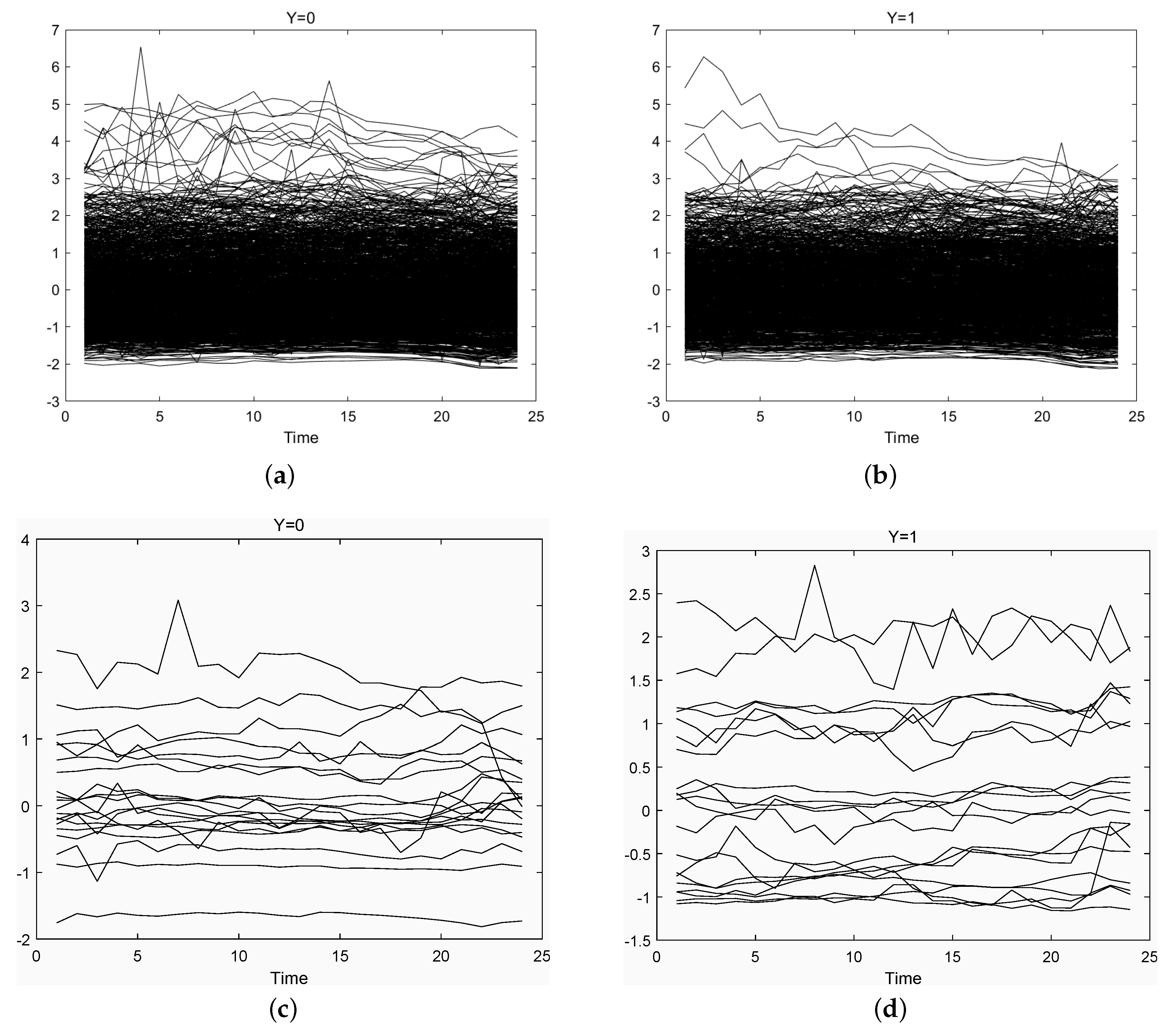
For simplicity, we standardize all the price data. For each group, we plot the housing price trajectories in Figure 1. Failure to visually detect differences between the groups could result from overcrowding of these plots with too many curves, but when displaying fewer curves (lower panels of Figure 1), the same phenomenon remains. With a few exceptions, no clear visual differences between the two groups can be discerned. On the whole, the trajectories of per year from 2015 to 2016 are not much different. Therefore, the discrimination task at hand is difficult.
We randomly select 75% of all residential areas as the training set with size 1739, and the rest as the testing data with size 579. We use logistic link and B-spline functions to fit the house price curves. The number of the basis functions is 6, and the order of the B-spline basis functions is 2. Then, we adopt functional principal component analysis (Yao et al. 2005) to built the data-adaptive basis functions to reduce the dimension and deal with the correlations in house price time series.
We compare the out-of-sample prediction errors of the seven methods in Section 4. We repeat every method 20 times. The results are summarized in Table 1 and Table 2. It can be observed from the tables that the error of CV1 or CV2 method is lower 10% on average than those of other methods, and overall, CV1 and CV2 behave similarly. As shown in the simulation above, this indicates the constraint that the sum of weights equals 1 makes sense in practical cases. AIC and BIC perform equally well, as both choose the largest model in most cases. We also find that FPCA is better than AIC or BIC. FPCA always selects the smallest model because the cumulative reliability of the first principal component is ~98%. Further, it is clear that the fitting error and prediction error of FPCA are similar. For the other methods, the fitting errors are always a little smaller than the prediction errors.
5. Concluding Remarks
In this paper, we proposed a model averaging approach under the framework of the generalized functional linear model. We showed that the weight chosen by the leave-one-out cross-validation method is asymptotically optimal in the sense of achieving the lowest possible squared error in a class of model averaging estimators. It can be seen from the theoretical proof that our method is also valid for the non-nested candidate model set. Numerical analysis shows that for generalized functional linear model, cross-validation model averaging is a powerful tool for estimation and prediction. A further work is to develop model averaging inference procedures based on generalized functional linear model. In addition, how to combine other covariates into generalized functional linear model is also an interesting problem.
Author Contributions
H.Z. wrote the original draft. G.Z. reviewed and revised the whole paper. All authors have read and agreed to the published version of the manuscript.
Funding
Zou’s work was partially supported by the Ministry of Science and Technology of China (Grant No. 2016YFB0502301) and the National Natural Science Foundation of China (Grant Nos. 11971323 and 11529101).
Acknowledgments
The authors thank the two referees for their constructive comments and suggestions that have substantially improved the original manuscript. The Beijing second-hand house price data is collected by the Guoxinda Group Corporation. This project was partially supported by the National Natural Science Foundation of China (Grant No.71571180).
Conflicts of Interest
The authors declare no conflicts of interest.
Appendix A. Lemmas and Proofs
The following Definition A1 and Lemma A1 can be found in Kahane (1968); Hoffmann (1974); Hoffmann and Pisier (1976); Zinn (1977); and Wu (1981).
Definition A1.
A linear map is of type 2 if converges in a.s. for all sequences such that , where and are Banach space, are independent random variables such that , and a.s. means converges almost surely. A Banach space is said to be type 2 if the identity map on is type 2.
Let be a compact metric space and be the Banach space of real-valued continuous functions on S with the supremum norm
for any . Denote a d-continuous metric on S. Let denote the minimal number of -balls of radius less than or equal to which cover S, and set
We let
and for , we define
where is some fixed point in S. In addition, assume that and are independent real-valued random variables. Then, are independent -valued random variables.
Lemma A1.
Let denote a compact metric space. Suppose that ρ is a d-continuous metric on S with
Then we have such that for all n,
where are independent -valued random variables with mean zeros.
Lemma A2.
For any , define
Under Condition 3, we have
Proof of Lemma A2.
First note that for any , we have
where the last step is by the mean-value theorem and is a point betweeen and . From the assumptions that is a twice continuously differentiable function with bounded derivatives and , and is strictly positive with bound and , we see that there is a constant such that , and
where the second inequality is by Cauchy–Schwarz inequality. Therefore, we obtain
As is a compact subset of , and is the Euclidean metric in , (A1) is satisfied. Thus, by Lemma A1, there is a constant uniformly for all l such that for any , we have
Notice
Therefore, for any , letting , we obtain
which implies (A3). □
Lemma A3.
Proof of Lemma A3.
By the definition of and Condition 6, then we have
where is a point between and . Recalling that
we obtain
where . From (A6), we get
By Condition 1, for any , there is an such that for all , we have
Lemma A4.
Under Conditions 1–4 and 6,
Appendix B. Proof of Theorem 1
Let , and
As in Li (1987) and Ando and Li (2014), we know that
As minimizes over , it also minimizes over . Therefore, the claim
is valid if
and
hold. In fact, if we denote , then
so we only need to prove
where for , and . According to the definition of , we have . Then, by (A10), we obtain
which is equivalent to
From (A11) and (A12), we have
and
Therefore,
with , and
Thus, we obtain
In the following, we prove (A11) and (A12).
Appendix B.1. Proof of (A11)
Notice that
So,
Therefore, to prove (A11), it suffices to verify
By Lemma A4, we need only to show
Let be the point between and . Then, for any , we have
which, together with the assumption that is a twice continuously differentiable function with bounded derivatives implying , leads to
Thus, to prove (A13), it suffices to show
By Condition 5, for fixed M, we obtain
which, together with Condition 4, leads to (A14), and thus (A13) holds.
Appendix B.2. Proof of (A12)
As
it is sufficient to show
It is readily seen that
Thus, we need only to prove
and
The proof of (A15) is similar to that of Wu (1981). We denote a metric
which is on . Let be a compact metric space. Then is the Banach space of real-valued continuous functions on with the supremum norm
Let denote the minimal number of -balls of radius less than or equal to which cover , and set
We let
and for , we define
where is some fixed point in .
Recalling that , we have
where is a point between and . From the assumption , and Condition 3, we obtain
As for , using Lagrange theorem, we have
where is a point between and . Again, by Condition 3, , and the assumption , we obtain
For (A15), we have
where is an arbitrary constant. Since is a compact subset of , and is the Euclidean metric in , (A1) is satisfied. Therefore, by Lemma A1, we see that there is a constant such that for all n,
where the last equality is because of (A18), (A19) and . Therefore,
and (A15) holds.
Appendix C. Simulation Results in Section 4.1

Table A1.
Prediction errors with n = 60 in Case 1.
| R | AIC | BIC | FPCA | S-AIC | S-BIC | CV1 | CV2 | |
|---|---|---|---|---|---|---|---|---|
| Mean | 0.432 | 0.408 | 0.404 | 0.433 | 0.408 | 0.394 | 0.393 | |
| 1 | Median | 0.417 | 0.417 | 0.417 | 0.417 | 0.417 | 0.375 | 0.417 |
| Var | 0.023 | 0.023 | 0.020 | 0.023 | 0.024 | 0.023 | 0.021 | |
| Mean | 0.312 | 0.294 | 0.249 | 0.311 | 0.292 | 0.225 | 0.226 | |
| 2 | Median | 0.333 | 0.333 | 0.250 | 0.333 | 0.333 | 0.250 | 0.250 |
| Var | 0.013 | 0.013 | 0.016 | 0.013 | 0.013 | 0.013 | 0.013 | |
| Mean | 0.273 | 0.262 | 0.226 | 0.273 | 0.260 | 0.188 | 0.189 | |
| 3 | Median | 0.250 | 0.250 | 0.250 | 0.250 | 0.250 | 0.167 | 0.167 |
| Var | 0.017 | 0.017 | 0.015 | 0.017 | 0.017 | 0.016 | 0.015 | |
| Mean | 0.256 | 0.243 | 0.183 | 0.256 | 0.247 | 0.162 | 0.163 | |
| 4 | Median | 0.250 | 0.250 | 0.167 | 0.250 | 0.250 | 0.167 | 0.167 |
| Var | 0.018 | 0.017 | 0.011 | 0.018 | 0.017 | 0.013 | 0.013 | |
| Mean | 0.203 | 0.196 | 0.148 | 0.203 | 0.193 | 0.133 | 0.134 | |
| 5 | Median | 0.167 | 0.167 | 0.167 | 0.167 | 0.167 | 0.083 | 0.083 |
| Var | 0.014 | 0.014 | 0.011 | 0.014 | 0.013 | 0.009 | 0.009 | |
| Mean | 0.234 | 0.233 | 0.135 | 0.234 | 0.233 | 0.117 | 0.115 | |
| 6 | Median | 0.250 | 0.250 | 0.125 | 0.250 | 0.250 | 0.083 | 0.083 |
| Var | 0.016 | 0.016 | 0.010 | 0.016 | 0.016 | 0.010 | 0.010 | |
| Mean | 0.214 | 0.213 | 0.149 | 0.214 | 0.214 | 0.118 | 0.117 | |
| 7 | Median | 0.208 | 0.208 | 0.167 | 0.208 | 0.250 | 0.083 | 0.083 |
| Var | 0.014 | 0.015 | 0.010 | 0.014 | 0.015 | 0.009 | 0.008 | |
| Mean | 0.213 | 0.209 | 0.134 | 0.213 | 0.210 | 0.104 | 0.103 | |
| 8 | Median | 0.250 | 0.167 | 0.125 | 0.250 | 0.167 | 0.083 | 0.083 |
| Var | 0.012 | 0.012 | 0.009 | 0.012 | 0.012 | 0.008 | 0.008 | |
| Mean | 0.196 | 0.196 | 0.128 | 0.196 | 0.196 | 0.096 | 0.099 | |
| 9 | Median | 0.167 | 0.167 | 0.083 | 0.167 | 0.167 | 0.083 | 0.083 |
| Var | 0.014 | 0.014 | 0.012 | 0.014 | 0.015 | 0.008 | 0.008 | |
| Mean | 0.209 | 0.208 | 0.126 | 0.209 | 0.206 | 0.088 | 0.087 | |
| 10 | Median | 0.167 | 0.167 | 0.083 | 0.167 | 0.167 | 0.083 | 0.083 |
| Var | 0.016 | 0.016 | 0.009 | 0.016 | 0.016 | 0.006 | 0.006 |
Table A2.
Prediction errors with n = 200 in Case 1.
| R | AIC | BIC | FPCA | S-AIC | S-BIC | CV1 | CV2 | |
|---|---|---|---|---|---|---|---|---|
| Mean | 0.355 | 0.350 | 0.329 | 0.355 | 0.349 | 0.322 | 0.322 | |
| 1 | Median | 0.350 | 0.350 | 0.325 | 0.350 | 0.350 | 0.325 | 0.313 |
| Var | 0.006 | 0.007 | 0.007 | 0.006 | 0.007 | 0.006 | 0.006 | |
| Mean | 0.262 | 0.262 | 0.234 | 0.262 | 0.262 | 0.227 | 0.227 | |
| 2 | Median | 0.275 | 0.275 | 0.225 | 0.275 | 0.275 | 0.225 | 0.225 |
| Var | 0.005 | 0.005 | 0.004 | 0.005 | 0.005 | 0.004 | 0.004 | |
| Mean | 0.205 | 0.205 | 0.184 | 0.205 | 0.205 | 0.174 | 0.174 | |
| 3 | Median | 0.200 | 0.200 | 0.175 | 0.200 | 0.200 | 0.175 | 0.175 |
| Var | 0.005 | 0.005 | 0.004 | 0.005 | 0.005 | 0.003 | 0.003 | |
| Mean | 0.163 | 0.163 | 0.134 | 0.163 | 0.163 | 0.128 | 0.128 | |
| 4 | Median | 0.150 | 0.150 | 0.125 | 0.150 | 0.150 | 0.125 | 0.125 |
| Var | 0.004 | 0.004 | 0.003 | 0.004 | 0.004 | 0.003 | 0.003 | |
| Mean | 0.139 | 0.139 | 0.113 | 0.139 | 0.139 | 0.110 | 0.110 | |
| 5 | Median | 0.125 | 0.125 | 0.113 | 0.125 | 0.125 | 0.100 | 0.100 |
| Var | 0.003 | 0.003 | 0.003 | 0.003 | 0.003 | 0.002 | 0.002 | |
| Mean | 0.136 | 0.136 | 0.101 | 0.136 | 0.136 | 0.094 | 0.094 | |
| 6 | Median | 0.125 | 0.125 | 0.100 | 0.125 | 0.125 | 0.100 | 0.100 |
| Var | 0.003 | 0.003 | 0.002 | 0.003 | 0.003 | 0.002 | 0.002 | |
| Mean | 0.129 | 0.129 | 0.099 | 0.129 | 0.129 | 0.086 | 0.086 | |
| 7 | Median | 0.125 | 0.125 | 0.100 | 0.125 | 0.125 | 0.075 | 0.075 |
| Var | 0.003 | 0.003 | 0.003 | 0.003 | 0.003 | 0.002 | 0.002 | |
| Mean | 0.121 | 0.121 | 0.091 | 0.121 | 0.121 | 0.083 | 0.082 | |
| 8 | Median | 0.113 | 0.113 | 0.075 | 0.113 | 0.113 | 0.075 | 0.075 |
| Var | 0.003 | 0.003 | 0.002 | 0.003 | 0.003 | 0.002 | 0.002 | |
| Mean | 0.127 | 0.127 | 0.090 | 0.127 | 0.127 | 0.084 | 0.083 | |
| 9 | Median | 0.125 | 0.125 | 0.100 | 0.125 | 0.125 | 0.075 | 0.075 |
| Var | 0.003 | 0.003 | 0.002 | 0.003 | 0.003 | 0.002 | 0.002 | |
| Mean | 0.121 | 0.121 | 0.088 | 0.121 | 0.121 | 0.069 | 0.069 | |
| 10 | Median | 0.125 | 0.125 | 0.075 | 0.125 | 0.125 | 0.075 | 0.075 |
| Var | 0.003 | 0.003 | 0.002 | 0.003 | 0.003 | 0.002 | 0.002 |
Table A3.
Prediction errors with n = 500 in Case 1.
| R | AIC | BIC | FPCA | S-AIC | S-BIC | CV1 | CV2 | |
|---|---|---|---|---|---|---|---|---|
| Mean | 0.349 | 0.349 | 0.332 | 0.349 | 0.349 | 0.330 | 0.330 | |
| 1 | Median | 0.345 | 0.345 | 0.330 | 0.345 | 0.345 | 0.330 | 0.330 |
| Var | 0.002 | 0.002 | 0.002 | 0.002 | 0.002 | 0.002 | 0.002 | |
| Mean | 0.240 | 0.240 | 0.232 | 0.240 | 0.240 | 0.228 | 0.228 | |
| 2 | Median | 0.240 | 0.240 | 0.230 | 0.240 | 0.240 | 0.230 | 0.230 |
| Var | 0.001 | 0.001 | 0.002 | 0.001 | 0.001 | 0.002 | 0.002 | |
| Mean | 0.176 | 0.176 | 0.174 | 0.176 | 0.176 | 0.168 | 0.168 | |
| 3 | Median | 0.170 | 0.170 | 0.170 | 0.170 | 0.170 | 0.160 | 0.160 |
| Var | 0.002 | 0.002 | 0.001 | 0.002 | 0.002 | 0.001 | 0.001 | |
| Mean | 0.143 | 0.143 | 0.133 | 0.143 | 0.143 | 0.135 | 0.134 | |
| 4 | Median | 0.140 | 0.140 | 0.130 | 0.140 | 0.140 | 0.130 | 0.130 |
| Var | 0.001 | 0.001 | 0.001 | 0.001 | 0.001 | 0.001 | 0.001 | |
| Mean | 0.126 | 0.126 | 0.114 | 0.126 | 0.126 | 0.115 | 0.115 | |
| 5 | Median | 0.120 | 0.120 | 0.110 | 0.120 | 0.120 | 0.110 | 0.110 |
| Var | 0.001 | 0.001 | 0.001 | 0.001 | 0.001 | 0.001 | 0.001 | |
| Mean | 0.109 | 0.109 | 0.097 | 0.109 | 0.109 | 0.095 | 0.096 | |
| 6 | Median | 0.110 | 0.110 | 0.090 | 0.110 | 0.110 | 0.090 | 0.090 |
| Var | 0.001 | 0.001 | 0.001 | 0.001 | 0.001 | 0.001 | 0.001 | |
| Mean | 0.106 | 0.106 | 0.090 | 0.106 | 0.106 | 0.089 | 0.089 | |
| 7 | Median | 0.110 | 0.110 | 0.090 | 0.110 | 0.110 | 0.090 | 0.090 |
| Var | 0.001 | 0.001 | 0.001 | 0.001 | 0.001 | 0.001 | 0.001 | |
| Mean | 0.096 | 0.096 | 0.081 | 0.096 | 0.096 | 0.084 | 0.084 | |
| 8 | Median | 0.090 | 0.090 | 0.080 | 0.090 | 0.090 | 0.080 | 0.080 |
| Var | 0.001 | 0.001 | 0.001 | 0.001 | 0.001 | 0.001 | 0.001 | |
| Mean | 0.090 | 0.090 | 0.075 | 0.090 | 0.090 | 0.070 | 0.070 | |
| 9 | Median | 0.085 | 0.085 | 0.070 | 0.085 | 0.085 | 0.065 | 0.065 |
| Var | 0.001 | 0.001 | 0.001 | 0.001 | 0.001 | 0.001 | 0.001 | |
| Mean | 0.091 | 0.091 | 0.075 | 0.091 | 0.091 | 0.069 | 0.068 | |
| 10 | Median | 0.090 | 0.090 | 0.070 | 0.090 | 0.090 | 0.065 | 0.065 |
| Var | 0.001 | 0.001 | 0.001 | 0.001 | 0.001 | 0.001 | 0.001 |
Table A4.
Prediction errors with n = 60 in Case 2.
| R | AIC | BIC | FPCA | S-AIC | S-BIC | CV1 | CV2 | |
|---|---|---|---|---|---|---|---|---|
| Mean | 0.362 | 0.346 | 0.359 | 0.359 | 0.342 | 0.351 | 0.354 | |
| 1 | Median | 0.333 | 0.333 | 0.333 | 0.333 | 0.333 | 0.333 | 0.333 |
| Var | 0.021 | 0.021 | 0.021 | 0.021 | 0.021 | 0.021 | 0.022 | |
| Mean | 0.315 | 0.251 | 0.262 | 0.300 | 0.245 | 0.245 | 0.248 | |
| 2 | Median | 0.333 | 0.250 | 0.250 | 0.250 | 0.250 | 0.250 | 0.250 |
| Var | 0.020 | 0.016 | 0.016 | 0.019 | 0.015 | 0.015 | 0.016 | |
| Mean | 0.269 | 0.193 | 0.208 | 0.257 | 0.188 | 0.185 | 0.184 | |
| 3 | Median | 0.250 | 0.167 | 0.167 | 0.250 | 0.167 | 0.167 | 0.167 |
| Var | 0.016 | 0.014 | 0.014 | 0.015 | 0.013 | 0.012 | 0.013 | |
| Mean | 0.258 | 0.174 | 0.176 | 0.252 | 0.167 | 0.163 | 0.164 | |
| 4 | Median | 0.250 | 0.167 | 0.167 | 0.250 | 0.167 | 0.167 | 0.167 |
| Var | 0.018 | 0.013 | 0.012 | 0.017 | 0.013 | 0.012 | 0.012 | |
| Mean | 0.244 | 0.145 | 0.169 | 0.239 | 0.137 | 0.138 | 0.135 | |
| 5 | Median | 0.250 | 0.167 | 0.167 | 0.250 | 0.167 | 0.083 | 0.083 |
| Var | 0.017 | 0.010 | 0.013 | 0.017 | 0.010 | 0.011 | 0.011 | |
| Mean | 0.234 | 0.142 | 0.150 | 0.227 | 0.131 | 0.122 | 0.119 | |
| 6 | Median | 0.250 | 0.167 | 0.167 | 0.250 | 0.083 | 0.083 | 0.083 |
| Var | 0.018 | 0.010 | 0.012 | 0.017 | 0.010 | 0.009 | 0.009 | |
| Mean | 0.214 | 0.127 | 0.142 | 0.205 | 0.118 | 0.113 | 0.110 | |
| 7 | Median | 0.167 | 0.083 | 0.167 | 0.167 | 0.083 | 0.083 | 0.083 |
| Var | 0.016 | 0.011 | 0.012 | 0.016 | 0.010 | 0.009 | 0.009 | |
| Mean | 0.230 | 0.120 | 0.156 | 0.223 | 0.110 | 0.105 | 0.107 | |
| 8 | Median | 0.250 | 0.083 | 0.167 | 0.167 | 0.083 | 0.083 | 0.083 |
| Var | 0.018 | 0.010 | 0.014 | 0.017 | 0.009 | 0.009 | 0.010 | |
| Mean | 0.204 | 0.121 | 0.160 | 0.192 | 0.108 | 0.100 | 0.099 | |
| 9 | Median | 0.167 | 0.083 | 0.167 | 0.167 | 0.083 | 0.083 | 0.083 |
| Var | 0.017 | 0.009 | 0.016 | 0.016 | 0.009 | 0.008 | 0.008 | |
| Mean | 0.201 | 0.114 | 0.178 | 0.182 | 0.101 | 0.096 | 0.096 | |
| 10 | Median | 0.167 | 0.083 | 0.167 | 0.167 | 0.083 | 0.083 | 0.083 |
| Var | 0.019 | 0.010 | 0.017 | 0.019 | 0.009 | 0.008 | 0.008 |
Table A5.
Prediction errors with n = 200 in Case 2.
| R | AIC | BIC | FPCA | S-AIC | S-BIC | CV1 | CV2 | |
|---|---|---|---|---|---|---|---|---|
| Mean | 0.369 | 0.336 | 0.349 | 0.369 | 0.336 | 0.342 | 0.341 | |
| 1 | Median | 0.375 | 0.325 | 0.350 | 0.375 | 0.325 | 0.350 | 0.338 |
| Var | 0.007 | 0.007 | 0.006 | 0.006 | 0.007 | 0.006 | 0.006 | |
| Mean | 0.265 | 0.253 | 0.239 | 0.265 | 0.248 | 0.233 | 0.233 | |
| 2 | Median | 0.275 | 0.250 | 0.250 | 0.275 | 0.250 | 0.225 | 0.225 |
| Var | 0.006 | 0.005 | 0.005 | 0.006 | 0.005 | 0.005 | 0.005 | |
| Mean | 0.204 | 0.204 | 0.184 | 0.204 | 0.203 | 0.175 | 0.175 | |
| 3 | Median | 0.200 | 0.200 | 0.175 | 0.200 | 0.200 | 0.175 | 0.175 |
| Var | 0.004 | 0.004 | 0.003 | 0.004 | 0.004 | 0.003 | 0.003 | |
| Mean | 0.175 | 0.175 | 0.147 | 0.175 | 0.175 | 0.143 | 0.142 | |
| 4 | Median | 0.175 | 0.175 | 0.150 | 0.175 | 0.175 | 0.150 | 0.125 |
| Var | 0.004 | 0.004 | 0.004 | 0.004 | 0.004 | 0.004 | 0.003 | |
| Mean | 0.157 | 0.157 | 0.130 | 0.157 | 0.157 | 0.118 | 0.118 | |
| 5 | Median | 0.150 | 0.150 | 0.125 | 0.150 | 0.150 | 0.125 | 0.125 |
| Var | 0.004 | 0.004 | 0.003 | 0.004 | 0.004 | 0.003 | 0.003 | |
| Mean | 0.148 | 0.148 | 0.120 | 0.148 | 0.148 | 0.108 | 0.107 | |
| 6 | Median | 0.150 | 0.150 | 0.125 | 0.150 | 0.150 | 0.100 | 0.100 |
| Var | 0.004 | 0.004 | 0.003 | 0.004 | 0.004 | 0.002 | 0.002 | |
| Mean | 0.150 | 0.150 | 0.116 | 0.150 | 0.150 | 0.092 | 0.091 | |
| 7 | Median | 0.150 | 0.150 | 0.113 | 0.150 | 0.150 | 0.100 | 0.100 |
| Var | 0.003 | 0.003 | 0.003 | 0.003 | 0.004 | 0.002 | 0.002 | |
| Mean | 0.162 | 0.161 | 0.125 | 0.162 | 0.161 | 0.091 | 0.092 | |
| 8 | Median | 0.150 | 0.150 | 0.125 | 0.150 | 0.150 | 0.088 | 0.100 |
| Var | 0.005 | 0.005 | 0.004 | 0.005 | 0.005 | 0.002 | 0.002 | |
| Mean | 0.173 | 0.167 | 0.130 | 0.173 | 0.165 | 0.086 | 0.087 | |
| 9 | Median | 0.175 | 0.175 | 0.125 | 0.175 | 0.150 | 0.075 | 0.075 |
| Var | 0.004 | 0.004 | 0.004 | 0.004 | 0.004 | 0.002 | 0.002 | |
| Mean | 0.192 | 0.172 | 0.147 | 0.192 | 0.167 | 0.088 | 0.090 | |
| 10 | Median | 0.200 | 0.175 | 0.150 | 0.200 | 0.150 | 0.075 | 0.075 |
| Var | 0.006 | 0.005 | 0.005 | 0.006 | 0.005 | 0.002 | 0.002 |
Table A6.
Prediction errors with n = 500 in Case 2.
| R | AIC | BIC | FPCA | S-AIC | S-BIC | CV1 | CV2 | |
|---|---|---|---|---|---|---|---|---|
| Mean | 0.345 | 0.338 | 0.332 | 0.345 | 0.336 | 0.330 | 0.330 | |
| 1 | Median | 0.350 | 0.340 | 0.330 | 0.350 | 0.340 | 0.330 | 0.330 |
| Var | 0.003 | 0.002 | 0.002 | 0.003 | 0.002 | 0.002 | 0.002 | |
| Mean | 0.239 | 0.239 | 0.227 | 0.239 | 0.239 | 0.225 | 0.225 | |
| 2 | Median | 0.240 | 0.240 | 0.230 | 0.240 | 0.240 | 0.225 | 0.220 |
| Var | 0.002 | 0.002 | 0.002 | 0.002 | 0.002 | 0.002 | 0.002 | |
| Mean | 0.182 | 0.182 | 0.170 | 0.182 | 0.182 | 0.168 | 0.168 | |
| 3 | Median | 0.180 | 0.180 | 0.170 | 0.180 | 0.180 | 0.170 | 0.170 |
| Var | 0.002 | 0.002 | 0.001 | 0.002 | 0.002 | 0.001 | 0.001 | |
| Mean | 0.152 | 0.152 | 0.141 | 0.152 | 0.152 | 0.136 | 0.136 | |
| 4 | Median | 0.150 | 0.150 | 0.140 | 0.150 | 0.150 | 0.140 | 0.140 |
| Var | 0.001 | 0.001 | 0.001 | 0.001 | 0.001 | 0.001 | 0.001 | |
| Mean | 0.135 | 0.135 | 0.120 | 0.135 | 0.135 | 0.114 | 0.114 | |
| 5 | Median | 0.130 | 0.130 | 0.120 | 0.130 | 0.130 | 0.110 | 0.110 |
| Var | 0.001 | 0.001 | 0.001 | 0.001 | 0.001 | 0.001 | 0.001 | |
| Mean | 0.129 | 0.129 | 0.110 | 0.129 | 0.129 | 0.100 | 0.101 | |
| 6 | Median | 0.130 | 0.130 | 0.110 | 0.130 | 0.130 | 0.100 | 0.100 |
| Var | 0.001 | 0.001 | 0.001 | 0.001 | 0.001 | 0.001 | 0.001 | |
| Mean | 0.128 | 0.128 | 0.107 | 0.128 | 0.128 | 0.092 | 0.093 | |
| 7 | Median | 0.130 | 0.130 | 0.100 | 0.130 | 0.130 | 0.090 | 0.090 |
| Var | 0.002 | 0.002 | 0.001 | 0.002 | 0.002 | 0.001 | 0.001 | |
| Mean | 0.134 | 0.134 | 0.109 | 0.134 | 0.134 | 0.086 | 0.087 | |
| 8 | Median | 0.130 | 0.130 | 0.110 | 0.130 | 0.130 | 0.080 | 0.080 |
| Var | 0.002 | 0.002 | 0.001 | 0.002 | 0.002 | 0.001 | 0.001 | |
| Mean | 0.147 | 0.147 | 0.117 | 0.147 | 0.147 | 0.086 | 0.088 | |
| 9 | Median | 0.140 | 0.140 | 0.110 | 0.140 | 0.140 | 0.090 | 0.090 |
| Var | 0.002 | 0.002 | 0.002 | 0.002 | 0.002 | 0.001 | 0.001 | |
| Mean | 0.171 | 0.171 | 0.135 | 0.171 | 0.171 | 0.093 | 0.096 | |
| 10 | Median | 0.170 | 0.170 | 0.135 | 0.170 | 0.170 | 0.090 | 0.090 |
| Var | 0.003 | 0.003 | 0.002 | 0.003 | 0.003 | 0.001 | 0.001 |
Table A7.
Prediction errors with n = 60 in Case 3.
| R | AIC | BIC | FPCA | S-AIC | S-BIC | CV1 | CV2 | |
|---|---|---|---|---|---|---|---|---|
| Mean | 0.494 | 0.482 | 0.430 | 0.490 | 0.483 | 0.405 | 0.413 | |
| 1 | Median | 0.500 | 0.500 | 0.417 | 0.500 | 0.500 | 0.417 | 0.417 |
| Var | 0.026 | 0.029 | 0.026 | 0.027 | 0.029 | 0.022 | 0.022 | |
| Mean | 0.428 | 0.412 | 0.317 | 0.427 | 0.412 | 0.318 | 0.303 | |
| 2 | Median | 0.417 | 0.417 | 0.333 | 0.417 | 0.417 | 0.333 | 0.333 |
| Var | 0.021 | 0.023 | 0.028 | 0.021 | 0.023 | 0.018 | 0.018 | |
| Mean | 0.416 | 0.401 | 0.317 | 0.419 | 0.403 | 0.313 | 0.302 | |
| 3 | Median | 0.417 | 0.417 | 0.292 | 0.417 | 0.417 | 0.292 | 0.250 |
| Var | 0.028 | 0.031 | 0.037 | 0.027 | 0.030 | 0.032 | 0.031 | |
| Mean | 0.424 | 0.387 | 0.393 | 0.420 | 0.382 | 0.357 | 0.344 | |
| 4 | Median | 0.500 | 0.417 | 0.417 | 0.458 | 0.417 | 0.333 | 0.333 |
| Var | 0.047 | 0.048 | 0.056 | 0.044 | 0.046 | 0.046 | 0.043 | |
| Mean | 0.372 | 0.362 | 0.493 | 0.398 | 0.365 | 0.380 | 0.355 | |
| 5 | Median | 0.333 | 0.333 | 0.583 | 0.417 | 0.333 | 0.417 | 0.333 |
| Var | 0.052 | 0.054 | 0.067 | 0.049 | 0.052 | 0.053 | 0.048 | |
| Mean | 0.400 | 0.383 | 0.608 | 0.427 | 0.390 | 0.446 | 0.430 | |
| 6 | Median | 0.417 | 0.375 | 0.667 | 0.417 | 0.375 | 0.500 | 0.417 |
| Var | 0.072 | 0.075 | 0.060 | 0.066 | 0.075 | 0.067 | 0.066 | |
| Mean | 0.374 | 0.378 | 0.628 | 0.428 | 0.388 | 0.481 | 0.468 | |
| 7 | Median | 0.333 | 0.333 | 0.667 | 0.417 | 0.417 | 0.500 | 0.500 |
| Var | 0.072 | 0.075 | 0.052 | 0.063 | 0.072 | 0.067 | 0.070 | |
| Mean | 0.457 | 0.457 | 0.673 | 0.527 | 0.474 | 0.615 | 0.593 | |
| 8 | Median | 0.417 | 0.417 | 0.750 | 0.583 | 0.500 | 0.667 | 0.667 |
| Var | 0.098 | 0.098 | 0.053 | 0.071 | 0.091 | 0.073 | 0.075 | |
| Mean | 0.565 | 0.565 | 0.738 | 0.642 | 0.583 | 0.652 | 0.659 | |
| 9 | Median | 0.583 | 0.583 | 0.750 | 0.750 | 0.667 | 0.750 | 0.750 |
| Var | 0.099 | 0.099 | 0.040 | 0.079 | 0.087 | 0.072 | 0.074 | |
| Mean | 0.565 | 0.565 | 0.744 | 0.662 | 0.613 | 0.698 | 0.694 | |
| 10 | Median | 0.583 | 0.583 | 0.750 | 0.667 | 0.667 | 0.750 | 0.750 |
| Var | 0.096 | 0.096 | 0.037 | 0.063 | 0.080 | 0.057 | 0.065 |
Table A8.
Prediction errors with n = 200 in Case 3.
| R | AIC | BIC | FPCA | S-AIC | S-BIC | CV1 | CV2 | |
|---|---|---|---|---|---|---|---|---|
| Mean | 0.406 | 0.403 | 0.366 | 0.406 | 0.401 | 0.341 | 0.342 | |
| 1 | Median | 0.400 | 0.400 | 0.350 | 0.400 | 0.400 | 0.325 | 0.325 |
| Var | 0.006 | 0.007 | 0.007 | 0.006 | 0.007 | 0.007 | 0.007 | |
| Mean | 0.378 | 0.377 | 0.310 | 0.378 | 0.378 | 0.272 | 0.271 | |
| 2 | Median | 0.375 | 0.375 | 0.300 | 0.375 | 0.375 | 0.250 | 0.250 |
| Var | 0.010 | 0.010 | 0.010 | 0.010 | 0.010 | 0.008 | 0.007 | |
| Mean | 0.428 | 0.428 | 0.324 | 0.428 | 0.427 | 0.253 | 0.251 | |
| 3 | Median | 0.463 | 0.463 | 0.300 | 0.463 | 0.450 | 0.225 | 0.225 |
| Var | 0.018 | 0.018 | 0.016 | 0.018 | 0.018 | 0.010 | 0.009 | |
| Mean | 0.465 | 0.427 | 0.370 | 0.470 | 0.430 | 0.259 | 0.254 | |
| 4 | Median | 0.500 | 0.475 | 0.350 | 0.500 | 0.475 | 0.225 | 0.225 |
| Var | 0.031 | 0.035 | 0.029 | 0.030 | 0.034 | 0.021 | 0.020 | |
| Mean | 0.281 | 0.231 | 0.507 | 0.310 | 0.228 | 0.282 | 0.276 | |
| 5 | Median | 0.200 | 0.175 | 0.500 | 0.225 | 0.175 | 0.238 | 0.225 |
| Var | 0.035 | 0.021 | 0.041 | 0.034 | 0.020 | 0.030 | 0.029 | |
| Mean | 0.242 | 0.242 | 0.612 | 0.289 | 0.242 | 0.325 | 0.321 | |
| 6 | Median | 0.175 | 0.175 | 0.675 | 0.225 | 0.175 | 0.238 | 0.238 |
| Var | 0.040 | 0.040 | 0.036 | 0.039 | 0.037 | 0.050 | 0.049 | |
| Mean | 0.298 | 0.298 | 0.712 | 0.363 | 0.294 | 0.368 | 0.362 | |
| 7 | Median | 0.200 | 0.200 | 0.725 | 0.313 | 0.200 | 0.300 | 0.288 |
| Var | 0.059 | 0.059 | 0.014 | 0.056 | 0.056 | 0.064 | 0.063 | |
| Mean | 0.476 | 0.476 | 0.749 | 0.553 | 0.473 | 0.498 | 0.495 | |
| 8 | Median | 0.513 | 0.513 | 0.763 | 0.588 | 0.500 | 0.588 | 0.575 |
| Var | 0.086 | 0.086 | 0.009 | 0.068 | 0.084 | 0.076 | 0.076 | |
| Mean | 0.497 | 0.497 | 0.785 | 0.625 | 0.500 | 0.592 | 0.586 | |
| 9 | Median | 0.525 | 0.525 | 0.800 | 0.700 | 0.538 | 0.663 | 0.650 |
| Var | 0.104 | 0.104 | 0.005 | 0.057 | 0.099 | 0.062 | 0.064 | |
| Mean | 0.606 | 0.606 | 0.807 | 0.746 | 0.627 | 0.662 | 0.661 | |
| 10 | Median | 0.750 | 0.750 | 0.825 | 0.825 | 0.800 | 0.763 | 0.750 |
| Var | 0.105 | 0.105 | 0.004 | 0.042 | 0.101 | 0.053 | 0.054 |
Table A9.
Prediction errors with n = 500 in Case 3.
| R | AIC | BIC | FPCA | S-AIC | S-BIC | CV1 | CV2 | |
|---|---|---|---|---|---|---|---|---|
| Mean | 0.394 | 0.394 | 0.360 | 0.394 | 0.394 | 0.338 | 0.338 | |
| 1 | Median | 0.390 | 0.390 | 0.355 | 0.390 | 0.390 | 0.340 | 0.340 |
| Var | 0.004 | 0.004 | 0.003 | 0.004 | 0.004 | 0.003 | 0.003 | |
| Mean | 0.345 | 0.345 | 0.280 | 0.345 | 0.345 | 0.241 | 0.244 | |
| 2 | Median | 0.340 | 0.340 | 0.275 | 0.340 | 0.340 | 0.240 | 0.240 |
| Var | 0.005 | 0.005 | 0.003 | 0.005 | 0.005 | 0.002 | 0.002 | |
| Mean | 0.426 | 0.426 | 0.286 | 0.426 | 0.426 | 0.190 | 0.200 | |
| 3 | Median | 0.430 | 0.430 | 0.270 | 0.430 | 0.430 | 0.190 | 0.200 |
| Var | 0.008 | 0.008 | 0.008 | 0.008 | 0.008 | 0.002 | 0.002 | |
| Mean | 0.524 | 0.490 | 0.390 | 0.526 | 0.490 | 0.170 | 0.190 | |
| 4 | Median | 0.550 | 0.540 | 0.400 | 0.550 | 0.540 | 0.160 | 0.180 |
| Var | 0.017 | 0.025 | 0.018 | 0.015 | 0.025 | 0.002 | 0.003 | |
| Mean | 0.225 | 0.199 | 0.535 | 0.241 | 0.198 | 0.168 | 0.170 | |
| 5 | Median | 0.160 | 0.160 | 0.560 | 0.180 | 0.160 | 0.150 | 0.160 |
| Var | 0.028 | 0.018 | 0.017 | 0.027 | 0.018 | 0.006 | 0.006 | |
| Mean | 0.186 | 0.183 | 0.665 | 0.225 | 0.184 | 0.183 | 0.183 | |
| 6 | Median | 0.140 | 0.140 | 0.680 | 0.180 | 0.140 | 0.140 | 0.150 |
| Var | 0.014 | 0.013 | 0.009 | 0.014 | 0.012 | 0.013 | 0.011 | |
| Mean | 0.251 | 0.251 | 0.735 | 0.322 | 0.252 | 0.251 | 0.253 | |
| 7 | Median | 0.170 | 0.170 | 0.740 | 0.260 | 0.170 | 0.170 | 0.190 |
| Var | 0.033 | 0.033 | 0.004 | 0.028 | 0.031 | 0.033 | 0.028 | |
| Mean | 0.376 | 0.376 | 0.776 | 0.511 | 0.379 | 0.376 | 0.383 | |
| 8 | Median | 0.335 | 0.335 | 0.780 | 0.520 | 0.335 | 0.335 | 0.385 |
| Var | 0.065 | 0.065 | 0.002 | 0.048 | 0.062 | 0.065 | 0.057 | |
| Mean | 0.467 | 0.467 | 0.797 | 0.650 | 0.476 | 0.467 | 0.491 | |
| 9 | Median | 0.475 | 0.475 | 0.800 | 0.700 | 0.480 | 0.475 | 0.510 |
| Var | 0.087 | 0.087 | 0.002 | 0.039 | 0.082 | 0.087 | 0.076 | |
| Mean | 0.652 | 0.652 | 0.822 | 0.820 | 0.675 | 0.652 | 0.713 | |
| 10 | Median | 0.780 | 0.780 | 0.820 | 0.840 | 0.790 | 0.780 | 0.800 |
| Var | 0.071 | 0.071 | 0.002 | 0.012 | 0.062 | 0.071 | 0.048 |
Table A10.
Prediction errors with n = 60 in Case 4.
| R | AIC | BIC | FPCA | S-AIC | S-BIC | CV1 | CV2 | |
|---|---|---|---|---|---|---|---|---|
| Mean | 0.389 | 0.378 | 0.417 | 0.396 | 0.381 | 0.381 | 0.387 | |
| 1 | Median | 0.417 | 0.333 | 0.417 | 0.417 | 0.417 | 0.417 | 0.417 |
| Var | 0.024 | 0.024 | 0.023 | 0.023 | 0.023 | 0.022 | 0.024 | |
| Mean | 0.286 | 0.268 | 0.363 | 0.299 | 0.269 | 0.268 | 0.268 | |
| 2 | Median | 0.250 | 0.250 | 0.333 | 0.250 | 0.250 | 0.250 | 0.250 |
| Var | 0.022 | 0.021 | 0.029 | 0.022 | 0.022 | 0.021 | 0.021 | |
| Mean | 0.230 | 0.219 | 0.382 | 0.259 | 0.228 | 0.219 | 0.219 | |
| 3 | Median | 0.167 | 0.167 | 0.333 | 0.250 | 0.167 | 0.167 | 0.167 |
| Var | 0.024 | 0.023 | 0.040 | 0.024 | 0.023 | 0.023 | 0.023 | |
| Mean | 0.186 | 0.181 | 0.460 | 0.242 | 0.199 | 0.181 | 0.181 | |
| 4 | Median | 0.167 | 0.167 | 0.417 | 0.167 | 0.167 | 0.167 | 0.167 |
| Var | 0.022 | 0.022 | 0.048 | 0.031 | 0.024 | 0.022 | 0.022 | |
| Mean | 0.195 | 0.194 | 0.545 | 0.284 | 0.216 | 0.194 | 0.194 | |
| 5 | Median | 0.167 | 0.167 | 0.583 | 0.250 | 0.167 | 0.167 | 0.167 |
| Var | 0.029 | 0.030 | 0.054 | 0.046 | 0.034 | 0.030 | 0.030 | |
| Mean | 0.213 | 0.211 | 0.642 | 0.374 | 0.256 | 0.211 | 0.211 | |
| 6 | Median | 0.167 | 0.167 | 0.667 | 0.333 | 0.167 | 0.167 | 0.167 |
| Var | 0.042 | 0.042 | 0.045 | 0.062 | 0.049 | 0.042 | 0.042 | |
| Mean | 0.208 | 0.210 | 0.680 | 0.424 | 0.268 | 0.210 | 0.210 | |
| 7 | Median | 0.167 | 0.167 | 0.750 | 0.417 | 0.167 | 0.167 | 0.167 |
| Var | 0.052 | 0.053 | 0.037 | 0.068 | 0.060 | 0.053 | 0.053 | |
| Mean | 0.228 | 0.228 | 0.727 | 0.513 | 0.310 | 0.228 | 0.228 | |
| 8 | Median | 0.167 | 0.167 | 0.750 | 0.500 | 0.250 | 0.167 | 0.167 |
| Var | 0.059 | 0.059 | 0.025 | 0.067 | 0.071 | 0.059 | 0.059 | |
| Mean | 0.259 | 0.258 | 0.730 | 0.572 | 0.366 | 0.258 | 0.258 | |
| 9 | Median | 0.167 | 0.167 | 0.750 | 0.583 | 0.250 | 0.167 | 0.167 |
| Var | 0.084 | 0.084 | 0.030 | 0.069 | 0.091 | 0.084 | 0.084 | |
| Mean | 0.303 | 0.303 | 0.761 | 0.665 | 0.455 | 0.303 | 0.303 | |
| 10 | Median | 0.167 | 0.167 | 0.750 | 0.750 | 0.417 | 0.167 | 0.167 |
| Var | 0.099 | 0.099 | 0.020 | 0.047 | 0.096 | 0.099 | 0.099 |
Table A11.
Prediction errors with n = 200 in Case 4.
| R | AIC | BIC | FPCA | S-AIC | S-BIC | CV1 | CV2 | |
|---|---|---|---|---|---|---|---|---|
| Mean | 0.378 | 0.348 | 0.387 | 0.380 | 0.350 | 0.354 | 0.353 | |
| 1 | Median | 0.375 | 0.350 | 0.375 | 0.375 | 0.350 | 0.350 | 0.350 |
| Var | 0.008 | 0.008 | 0.008 | 0.008 | 0.007 | 0.007 | 0.007 | |
| Mean | 0.277 | 0.251 | 0.330 | 0.287 | 0.253 | 0.258 | 0.258 | |
| 2 | Median | 0.275 | 0.250 | 0.325 | 0.275 | 0.250 | 0.250 | 0.250 |
| Var | 0.007 | 0.006 | 0.010 | 0.007 | 0.006 | 0.007 | 0.006 | |
| Mean | 0.193 | 0.183 | 0.374 | 0.216 | 0.186 | 0.205 | 0.205 | |
| 3 | Median | 0.175 | 0.175 | 0.375 | 0.200 | 0.175 | 0.200 | 0.200 |
| Var | 0.006 | 0.005 | 0.020 | 0.007 | 0.005 | 0.006 | 0.006 | |
| Mean | 0.168 | 0.167 | 0.512 | 0.219 | 0.171 | 0.217 | 0.216 | |
| 4 | Median | 0.150 | 0.150 | 0.550 | 0.200 | 0.150 | 0.200 | 0.200 |
| Var | 0.008 | 0.008 | 0.022 | 0.012 | 0.008 | 0.011 | 0.011 | |
| Mean | 0.141 | 0.141 | 0.613 | 0.237 | 0.152 | 0.237 | 0.237 | |
| 5 | Median | 0.125 | 0.125 | 0.650 | 0.200 | 0.125 | 0.200 | 0.200 |
| Var | 0.008 | 0.008 | 0.020 | 0.019 | 0.009 | 0.018 | 0.018 | |
| Mean | 0.132 | 0.132 | 0.700 | 0.294 | 0.146 | 0.292 | 0.291 | |
| 6 | Median | 0.100 | 0.100 | 0.700 | 0.250 | 0.125 | 0.250 | 0.250 |
| Var | 0.011 | 0.011 | 0.010 | 0.030 | 0.013 | 0.029 | 0.029 | |
| Mean | 0.138 | 0.138 | 0.742 | 0.392 | 0.161 | 0.381 | 0.377 | |
| 7 | Median | 0.100 | 0.100 | 0.750 | 0.375 | 0.125 | 0.375 | 0.375 |
| Var | 0.014 | 0.014 | 0.007 | 0.039 | 0.017 | 0.033 | 0.033 | |
| Mean | 0.154 | 0.154 | 0.769 | 0.512 | 0.193 | 0.490 | 0.487 | |
| 8 | Median | 0.100 | 0.100 | 0.775 | 0.550 | 0.125 | 0.500 | 0.500 |
| Var | 0.023 | 0.023 | 0.004 | 0.042 | 0.028 | 0.039 | 0.039 | |
| Mean | 0.175 | 0.175 | 0.788 | 0.624 | 0.232 | 0.583 | 0.580 | |
| 9 | Median | 0.100 | 0.100 | 0.800 | 0.675 | 0.125 | 0.625 | 0.625 |
| Var | 0.038 | 0.038 | 0.005 | 0.032 | 0.046 | 0.035 | 0.035 | |
| Mean | 0.192 | 0.192 | 0.800 | 0.695 | 0.282 | 0.654 | 0.653 | |
| 10 | Median | 0.100 | 0.100 | 0.800 | 0.725 | 0.175 | 0.688 | 0.675 |
| Var | 0.049 | 0.049 | 0.004 | 0.024 | 0.063 | 0.029 | 0.029 |
Table A12.
Prediction errors with n = 500 in Case 4.
| R | AIC | BIC | FPCA | S-AIC | S-BIC | CV1 | CV2 | |
|---|---|---|---|---|---|---|---|---|
| Mean | 0.380 | 0.339 | 0.367 | 0.380 | 0.340 | 0.338 | 0.339 | |
| 1 | Median | 0.380 | 0.340 | 0.360 | 0.380 | 0.340 | 0.340 | 0.340 |
| Var | 0.003 | 0.003 | 0.004 | 0.003 | 0.003 | 0.003 | 0.003 | |
| Mean | 0.278 | 0.242 | 0.310 | 0.284 | 0.242 | 0.228 | 0.229 | |
| 2 | Median | 0.270 | 0.240 | 0.300 | 0.280 | 0.240 | 0.230 | 0.230 |
| Var | 0.005 | 0.003 | 0.005 | 0.004 | 0.003 | 0.002 | 0.002 | |
| Mean | 0.180 | 0.177 | 0.385 | 0.198 | 0.179 | 0.176 | 0.179 | |
| 3 | Median | 0.170 | 0.170 | 0.380 | 0.190 | 0.170 | 0.170 | 0.180 |
| Var | 0.002 | 0.002 | 0.009 | 0.003 | 0.002 | 0.002 | 0.002 | |
| Mean | 0.141 | 0.141 | 0.527 | 0.184 | 0.143 | 0.141 | 0.146 | |
| 4 | Median | 0.140 | 0.140 | 0.540 | 0.170 | 0.140 | 0.140 | 0.140 |
| Var | 0.001 | 0.001 | 0.010 | 0.003 | 0.001 | 0.001 | 0.001 | |
| Mean | 0.122 | 0.122 | 0.649 | 0.203 | 0.126 | 0.122 | 0.130 | |
| 5 | Median | 0.120 | 0.120 | 0.660 | 0.185 | 0.120 | 0.120 | 0.120 |
| Var | 0.002 | 0.002 | 0.004 | 0.007 | 0.002 | 0.002 | 0.002 | |
| Mean | 0.109 | 0.109 | 0.716 | 0.266 | 0.116 | 0.109 | 0.125 | |
| 6 | Median | 0.100 | 0.100 | 0.720 | 0.240 | 0.110 | 0.100 | 0.110 |
| Var | 0.002 | 0.002 | 0.003 | 0.013 | 0.002 | 0.002 | 0.003 | |
| Mean | 0.103 | 0.103 | 0.754 | 0.371 | 0.115 | 0.103 | 0.129 | |
| 7 | Median | 0.090 | 0.090 | 0.750 | 0.360 | 0.100 | 0.090 | 0.120 |
| Var | 0.003 | 0.003 | 0.002 | 0.020 | 0.004 | 0.003 | 0.005 | |
| Mean | 0.102 | 0.102 | 0.775 | 0.490 | 0.119 | 0.102 | 0.141 | |
| 8 | Median | 0.090 | 0.090 | 0.780 | 0.500 | 0.100 | 0.090 | 0.120 |
| Var | 0.005 | 0.005 | 0.002 | 0.023 | 0.006 | 0.005 | 0.007 | |
| Mean | 0.112 | 0.112 | 0.791 | 0.629 | 0.143 | 0.112 | 0.184 | |
| 9 | Median | 0.090 | 0.090 | 0.790 | 0.650 | 0.110 | 0.090 | 0.140 |
| Var | 0.009 | 0.009 | 0.002 | 0.015 | 0.012 | 0.009 | 0.017 | |
| Mean | 0.114 | 0.114 | 0.802 | 0.707 | 0.155 | 0.114 | 0.211 | |
| 10 | Median | 0.080 | 0.080 | 0.800 | 0.720 | 0.110 | 0.080 | 0.160 |
| Var | 0.014 | 0.014 | 0.002 | 0.007 | 0.019 | 0.014 | 0.025 |
Appendix D. Simulation Results in Section 4.2
Table A13.
Prediction errors with .
| N | R = 1 | AIC | BIC | PCA | SAIC | SBIC | CV1 | CV2 |
|---|---|---|---|---|---|---|---|---|
| Mean | 0.329 | 0.325 | 0.312 | 0.323 | 0.322 | 0.313 | 0.313 | |
| 200 | Median | 0.325 | 0.325 | 0.300 | 0.325 | 0.325 | 0.325 | 0.325 |
| Var | 0.006 | 0.006 | 0.005 | 0.006 | 0.006 | 0.006 | 0.006 | |
| Mean | 0.330 | 0.319 | 0.305 | 0.327 | 0.314 | 0.304 | 0.304 | |
| 400 | Median | 0.325 | 0.313 | 0.300 | 0.325 | 0.313 | 0.300 | 0.300 |
| Var | 0.003 | 0.003 | 0.003 | 0.003 | 0.003 | 0.003 | 0.003 | |
| Mean | 0.332 | 0.326 | 0.304 | 0.330 | 0.326 | 0.305 | 0.304 | |
| 1000 | Median | 0.330 | 0.320 | 0.303 | 0.330 | 0.320 | 0.303 | 0.300 |
| Var | 0.001 | 0.001 | 0.001 | 0.001 | 0.001 | 0.001 | 0.001 |
Table A14.
Prediction errors with .
| N | R = 3 | AIC | BIC | PCA | SAIC | SBIC | CV1 | CV2 |
|---|---|---|---|---|---|---|---|---|
| Mean | 0.173 | 0.173 | 0.168 | 0.173 | 0.173 | 0.162 | 0.162 | |
| 200 | Median | 0.175 | 0.175 | 0.175 | 0.175 | 0.175 | 0.175 | 0.163 |
| Var | 0.003 | 0.003 | 0.002 | 0.003 | 0.003 | 0.002 | 0.002 | |
| Mean | 0.172 | 0.172 | 0.163 | 0.172 | 0.171 | 0.167 | 0.169 | |
| 400 | Median | 0.175 | 0.175 | 0.163 | 0.175 | 0.175 | 0.175 | 0.175 |
| Var | 0.001 | 0.001 | 0.002 | 0.001 | 0.001 | 0.001 | 0.002 | |
| Mean | 0.175 | 0.193 | 0.156 | 0.175 | 0.189 | 0.149 | 0.148 | |
| 1000 | Median | 0.180 | 0.198 | 0.160 | 0.180 | 0.190 | 0.145 | 0.145 |
| Var | 0.001 | 0.001 | 0.000 | 0.001 | 0.001 | 0.001 | 0.001 |
Table A15.
Prediction errors with .
| N | R = 7 | AIC | BIC | PCA | SAIC | SBIC | CV1 | CV2 |
|---|---|---|---|---|---|---|---|---|
| Mean | 0.104 | 0.104 | 0.109 | 0.104 | 0.104 | 0.095 | 0.097 | |
| 200 | Median | 0.100 | 0.100 | 0.100 | 0.100 | 0.100 | 0.100 | 0.088 |
| Var | 0.003 | 0.003 | 0.003 | 0.003 | 0.003 | 0.003 | 0.002 | |
| Mean | 0.106 | 0.106 | 0.101 | 0.106 | 0.106 | 0.087 | 0.087 | |
| 400 | Median | 0.100 | 0.100 | 0.100 | 0.100 | 0.100 | 0.088 | 0.088 |
| Var | 0.001 | 0.001 | 0.001 | 0.001 | 0.001 | 0.001 | 0.001 | |
| Mean | 0.109 | 0.109 | 0.103 | 0.109 | 0.109 | 0.084 | 0.083 | |
| 1000 | Median | 0.110 | 0.110 | 0.105 | 0.110 | 0.110 | 0.085 | 0.080 |
| Var | 0.001 | 0.001 | 0.000 | 0.001 | 0.001 | 0.000 | 0.000 |
References
- Ando, Tomohiro, and Ker Chau Li. 2014. A model-averaging approach for high-dimensional regression. Journal of the American Statistical Association 109: 254–65. [Google Scholar] [CrossRef]
- Ando, Tomohiro, and Ker Chau Li. 2017. A weight-relaxed model averaging approach for high-dimensional generalized linear models. The Annals of Statistics 45: 2654–79. [Google Scholar] [CrossRef]
- Andrews, Donald W. K. 1991. Asymptotic optimality of generalized CL, cross-validation, and generalized cross-validation in regression with heteroskedastic errors. Journal of Econometrics 47: 359–77. [Google Scholar] [CrossRef] [Green Version]
- Balan, Raluca M., and Ioana Schiopu-Kratina. 2005. Asymptotic results with generalized estimating equations for longitudinal data. The Annals of Statistics 33: 522–41. [Google Scholar] [CrossRef] [Green Version]
- Buckland, Steven T., Kenneth P. Burnham, and Nicole H. Augustin. 1997. Model selection: An integral part of inference. Biometrics 53: 603–18. [Google Scholar] [CrossRef]
- Chen, Kani, Inchi Hu, and Zhiliang Ying. 1999. Strong consistency of maximum quasi-likelihood estimators in generalized linear models with fixed and adaptive designs. The Annals of Statistics 27: 1155–63. [Google Scholar] [CrossRef]
- Claeskens, Gerda, and Raymond J. Carroll. 2007. An asymptotic theory for model selection inference in general semiparametric problems. Biometrika 94: 249–65. [Google Scholar] [CrossRef]
- Flynn, Cheryl J., Clifford M. Hurvich, and Jeffrey S. Simonoff. 2013. Efficiency for regularization parameter selection in penalized likelihood estimation of misspecified models. Journal of the American Statistical Association 108: 1031–43. [Google Scholar] [CrossRef] [Green Version]
- Gao, Yan, Xinyu Zhang, Shouyang Wang, and Guohua Zou. 2016. Model averaging based on leave-subject-out cross-validation. Journal of Econometrics 192: 139–51. [Google Scholar] [CrossRef]
- Hansen, Bruce E. 2007. Least squares model averaging. Econometrica 75: 1175–89. [Google Scholar] [CrossRef] [Green Version]
- Hansen, Bruce E., and Jeffrey S. Racine. 2012. Jacknife model averaging. Journal of Econometrics 167: 38–46. [Google Scholar] [CrossRef] [Green Version]
- Hoffmann-Jørgensen, Jørgen. 1974. Sums of independent Banach space valued random variables. Studia Mathematica 52: 159–86. [Google Scholar] [CrossRef] [Green Version]
- Hoffmann-Jørgensen, Jørgen, and Gilles Pisier. 1976. The law of large numbers and the central limit theorem in Banach spaces. The Annals of Probability 4: 587–99. [Google Scholar] [CrossRef]
- Hjort, Nils L., and Gerda Claeskens. 2003. Frequentist model average estimators. Journal of the American Statistical Association 98: 879–99. [Google Scholar] [CrossRef] [Green Version]
- James, Gareth M. 2002. Generalized linear models with functional predictors. Journal of the Royal Statistical Society: Series B (Statistical Methodology) 64: 411–32. [Google Scholar] [CrossRef]
- Kahane, Jean Pierrc. 1968. Some Random Series of Functions. Lexington: D. C. Heath. [Google Scholar]
- Li, Ker Chau. 1987. Asymptotic optimality for Cp,CL, cross-validation and generalized cross-validation: discrete index set. The Annals of Statistics 15: 958–75. [Google Scholar] [CrossRef]
- Liang, Hua, Guohua Zou, Alan T. K. Wan, and Xinyu Zhang. 2011. Optimal weight choice for frequentist model average estimators. Journal of the American Statistical Association 106: 1053–66. [Google Scholar] [CrossRef]
- Lv, Jinchi, and Jun S. Liu. 2014. Model selection principles in misspecified models. Journal of the Royal Statistical Society: Series B (Statistical Methodology) 76: 141–67. [Google Scholar] [CrossRef] [Green Version]
- Müller, Hans Georg, and Ulrich Stadtmüller. 2005. Generalized functional linear models. The Annals of Statistics 33: 774–805. [Google Scholar] [CrossRef] [Green Version]
- Wan, Alan T. K., Xinyu Zhang, and Guohua Zou. 2010. Least squares model averaging by Mallows criterion. Journal of Econometrics 156: 277–83. [Google Scholar] [CrossRef]
- Wu, Chien-Fu. 1981. Asymptotic theory of nonlinear least squares estimation. The Annals of Statistics 9: 501–13. [Google Scholar] [CrossRef]
- Xu, Ganggang, Suojin Wang, and Jianhua Z. Huang. 2014. Focused information criterion and model averaging based on weighted composite quantile regression. Scandinavian Journal of Statistics 41: 365–81. [Google Scholar] [CrossRef]
- Yang, Yuhong. 2001. Adaptive regression by mixing. Journal of the American Statistical Association 96: 574–88. [Google Scholar] [CrossRef] [Green Version]
- Yao, Fang, Müller Hans-Georg, and Wang Jane-Ling. 2005. Functional data analysis for sparse longitudinal data. Journal of the American Statistical Association 100: 577–90. [Google Scholar] [CrossRef]
- Zhang, Xinyu, and Hua Liang. 2011. Focused information criterion and model averaging for generalized additive partial linear models. The Annals of Statistics 39: 174–200. [Google Scholar] [CrossRef] [Green Version]
- Zhang, Xinyu, Alan T. K. Wan, and Sherry Z. Zhou. 2012. Focused information criteria model selection and model averaging in a Tobit model with a non-zero threshold. Journal of Business and Economic Statistics 30: 132–42. [Google Scholar] [CrossRef]
- Zhang, Xinyu, Alan T. K. Wan, and Guohua Zou. 2013. Model averaging by jackknife criterion in models with dependent data. Journal of Econometrics 174: 82–94. [Google Scholar] [CrossRef]
- Zhang, Xinyu. 2015. Consistency of model averaging estimators. Economics Letters 130: 120–23. [Google Scholar] [CrossRef]
- Zhang, Xinyu, Dalei Yu, Guohua Zou, and Hua Liang. 2016. Optimal model averaging estimation for generalized linear models and generalized Linear mixed-effects models. Journal of the American Statistical Association 111: 1775–90. [Google Scholar] [CrossRef]
- Zhang, Xinyu, Jeng-Min Chiou, and Yanyuan Ma. 2018. Functional prediction through averaging estimated functional linear regression models. Biometrika 105: 945–62. [Google Scholar] [CrossRef]
- Zhao, Shangwei, Jun Liao, and Dalei Yu. 2018. Model averaging estimator in ridge regression and its large sample properties. Statistical Papers. [Google Scholar] [CrossRef]
- Zhu, Rong, Guohua Zou, and Xinyu Zhang. 2018. Optimal model averaging estimation for partial functional linear models. Journal of Systems Science and Mathematical Sciences 38: 777–800. [Google Scholar]
- Zinn, Joel. 1977. A note on the central limit theorem in Banach spaces. The Annals of Probability 5: 283–86. [Google Scholar] [CrossRef]
Figure 1.
Predictor trajectories, corresponding to slightly smoothed monthly price curves. The low rising residential areas are in the upper left (a). The high rising residential areas are in upper right (b). Randomly selected profiles from the panels above are shown in the lower panels (c,d) for 20 districts.

Table 1.
Error of prediction.
| Rounds | AIC | BIC | FPCA | S-AIC | S-BIC | CV1 | CV2 |
|---|---|---|---|---|---|---|---|
| 1 | 0.301 | 0.301 | 0.275 | 0.301 | 0.301 | 0.221 | 0.221 |
| 2 | 0.292 | 0.292 | 0.247 | 0.292 | 0.292 | 0.178 | 0.176 |
| 3 | 0.290 | 0.290 | 0.242 | 0.290 | 0.290 | 0.187 | 0.187 |
| 4 | 0.280 | 0.280 | 0.233 | 0.280 | 0.280 | 0.176 | 0.174 |
| 5 | 0.276 | 0.276 | 0.233 | 0.276 | 0.276 | 0.147 | 0.149 |
| 6 | 0.316 | 0.316 | 0.233 | 0.316 | 0.316 | 0.188 | 0.188 |
| 7 | 0.269 | 0.269 | 0.244 | 0.269 | 0.269 | 0.164 | 0.164 |
| 8 | 0.294 | 0.294 | 0.225 | 0.294 | 0.294 | 0.174 | 0.174 |
| 9 | 0.316 | 0.316 | 0.235 | 0.316 | 0.316 | 0.187 | 0.187 |
| 10 | 0.282 | 0.282 | 0.242 | 0.282 | 0.282 | 0.174 | 0.173 |
| 11 | 0.292 | 0.292 | 0.240 | 0.292 | 0.292 | 0.162 | 0.162 |
| 12 | 0.285 | 0.285 | 0.261 | 0.285 | 0.285 | 0.188 | 0.188 |
| 13 | 0.282 | 0.282 | 0.219 | 0.282 | 0.282 | 0.150 | 0.149 |
| 14 | 0.264 | 0.264 | 0.280 | 0.264 | 0.264 | 0.188 | 0.188 |
| 15 | 0.282 | 0.282 | 0.247 | 0.282 | 0.282 | 0.187 | 0.187 |
| 16 | 0.295 | 0.295 | 0.269 | 0.295 | 0.295 | 0.185 | 0.185 |
| 17 | 0.328 | 0.328 | 0.252 | 0.328 | 0.328 | 0.204 | 0.202 |
| 18 | 0.301 | 0.301 | 0.245 | 0.301 | 0.301 | 0.187 | 0.187 |
| 19 | 0.278 | 0.278 | 0.209 | 0.278 | 0.278 | 0.150 | 0.150 |
| 20 | 0.311 | 0.311 | 0.249 | 0.311 | 0.311 | 0.183 | 0.183 |
Table 2.
Error of fitting.
| Rounds | AIC | BIC | FPCA | S-AIC | S-BIC | CV1 | CV2 |
|---|---|---|---|---|---|---|---|
| 1 | 0.287 | 0.287 | 0.235 | 0.287 | 0.287 | 0.166 | 0.165 |
| 2 | 0.289 | 0.289 | 0.244 | 0.289 | 0.289 | 0.181 | 0.180 |
| 3 | 0.290 | 0.290 | 0.246 | 0.290 | 0.290 | 0.174 | 0.173 |
| 4 | 0.293 | 0.293 | 0.249 | 0.293 | 0.293 | 0.182 | 0.182 |
| 5 | 0.296 | 0.296 | 0.249 | 0.296 | 0.296 | 0.190 | 0.190 |
| 6 | 0.285 | 0.285 | 0.249 | 0.285 | 0.285 | 0.175 | 0.175 |
| 7 | 0.297 | 0.297 | 0.246 | 0.297 | 0.297 | 0.184 | 0.183 |
| 8 | 0.292 | 0.292 | 0.252 | 0.292 | 0.292 | 0.179 | 0.179 |
| 9 | 0.283 | 0.283 | 0.248 | 0.283 | 0.283 | 0.174 | 0.173 |
| 10 | 0.291 | 0.291 | 0.246 | 0.291 | 0.291 | 0.182 | 0.181 |
| 11 | 0.291 | 0.291 | 0.247 | 0.291 | 0.291 | 0.184 | 0.186 |
| 12 | 0.294 | 0.294 | 0.240 | 0.294 | 0.294 | 0.175 | 0.175 |
| 13 | 0.293 | 0.293 | 0.254 | 0.293 | 0.293 | 0.190 | 0.187 |
| 14 | 0.295 | 0.295 | 0.233 | 0.295 | 0.295 | 0.175 | 0.175 |
| 15 | 0.293 | 0.293 | 0.244 | 0.293 | 0.293 | 0.176 | 0.177 |
| 16 | 0.288 | 0.288 | 0.237 | 0.288 | 0.288 | 0.179 | 0.178 |
| 17 | 0.282 | 0.282 | 0.243 | 0.282 | 0.282 | 0.173 | 0.173 |
| 18 | 0.290 | 0.290 | 0.245 | 0.290 | 0.290 | 0.178 | 0.177 |
| 19 | 0.294 | 0.294 | 0.257 | 0.294 | 0.294 | 0.186 | 0.187 |
| 20 | 0.285 | 0.285 | 0.244 | 0.285 | 0.285 | 0.179 | 0.179 |
© 2020 by the authors. Licensee MDPI, Basel, Switzerland. This article is an open access article distributed under the terms and conditions of the Creative Commons Attribution (CC BY) license (http://creativecommons.org/licenses/by/4.0/).
Share and Cite
MDPI and ACS Style
Zhang, H.; Zou, G. Cross-Validation Model Averaging for Generalized Functional Linear Model. Econometrics 2020, 8, 7. https://0-doi-org.brum.beds.ac.uk/10.3390/econometrics8010007
AMA Style
Zhang H, Zou G. Cross-Validation Model Averaging for Generalized Functional Linear Model. Econometrics. 2020; 8(1):7. https://0-doi-org.brum.beds.ac.uk/10.3390/econometrics8010007
Chicago/Turabian StyleZhang, Haili, and Guohua Zou. 2020. "Cross-Validation Model Averaging for Generalized Functional Linear Model" Econometrics 8, no. 1: 7. https://0-doi-org.brum.beds.ac.uk/10.3390/econometrics8010007
Note that from the first issue of 2016, this journal uses article numbers instead of page numbers. See further details here.