Balanced Growth Approach to Tracking Recessions

Department of Economics, University of Pittsburgh, 230 South Bouquet Street, Wesley W. Posvar Hall, Pittsburgh, PA 15213, USA
*
Author to whom correspondence should be addressed.
Econometrics 2020, 8(2), 14; https://doi.org/10.3390/econometrics8020014
Submission received: 3 October 2018
/
Revised: 8 April 2020
/
Accepted: 9 April 2020
/
Published: 23 April 2020
(This article belongs to the Special Issue Celebrated Econometricians: David Hendry)
Abstract
:In this paper, we propose a hybrid version of Dynamic Stochastic General Equilibrium models with an emphasis on parameter invariance and tracking performance at times of rapid changes (recessions). We interpret hypothetical balanced growth ratios as moving targets for economic agents that rely upon an Error Correction Mechanism to adjust to changes in target ratios driven by an underlying state Vector AutoRegressive process. Our proposal is illustrated by an application to a pilot Real Business Cycle model for the US economy from 1948 to 2019. An extensive recursive validation exercise over the last 35 years, covering 3 recessions, is used to highlight its parameters invariance, tracking and 1- to 3-step ahead forecasting performance, outperforming those of an unconstrained benchmark Vector AutoRegressive model.
1. Introduction
Dynamic Stochastic General Equilibrium (DSGE) models are generally justified on the grounds that they provide a structural foundation for policy analysis and are indeed widely used for that purpose. However, their tracking failures in times of rapid changes (such as the 2007–09 Great Recession) raise concerns relative to their relevance for policy recommendations in such times when they are most critically needed. Hence, there is a widely recognized need for greater diversification of the macroeconomics toolbox with models that focus on improved recession tracking performance, possibly at the cost of loosening the theoretical straitjacket of DSGE models.
In the present paper, we propose a generic procedure to transform DSGE models into hybrid versions thereof in a way that preserves their policy relevance while significantly improving their recession tracking performance. In particular, the approach we propose addresses the inherent “trade-off between theoretical and empirical coherence” (Pagan 2003) and can be applied to a wide range of DSGE models, covering various sectors of the economy. For empirical coherence, we rely upon an Error Correction Mechanism (ECM), which has repeatedly proved highly successful in modeling agents’ pursuit of moving targets represented by time-varying cointegration relationships. Simultaneously, in order to preserve theoretical coherence, we derive these targets as (moving) balanced growth solutions to the assumed model. This can be achieved without significantly weakening empirical coherence as theory models are designed to rationalize observed behavior and hence, there typically exists a close match between empirically derived cointegrating relationships and theory derived solutions.
In order to transform DSGE models into hybrid versions thereof, we implement four key modifications. First, we abandon assumptions of trend stationarity and rely instead on real (per capita) data that except for being seasonally adjusted are neither detrended nor Hodrick-Prescott (HP) filtered. Second, instead of computing conventional DSGE solutions based upon model consistent expectations of future values, we compute balanced growth solutions based upon agents’ perception of the growth scenario at any given point in time. Next, as we rely upon real data, we account for the fact that the balanced growth ratios vary significantly over time, to the extent that we are effectively treating these (theory-derived) moving targets as time-varying cointegration relationships. It follows that an appropriate subset of the model structural parameters can no longer be treated as time invariant. Instead, it is modeled as a set of state variables driven by a Vector AutoRegressive (VAR) process. Last but not least, we assume that agents rely upon an ECM process to track their moving targets.
In our approach, we draw a clear distinction between forecasting recessions and tracking them. As discussed further in our literature review, DSGE models that rely upon model consistent expectations are highly vulnerable to unexpected shocks. This is particularly critical for recessions since, as surveyed in Section 3, each postwar recession was triggered by a unique set of circumstances. This fundamentally prevents ex-ante econometric estimation of such potential triggers. Moreover, recession predictive failures can also extend to poor recession tracking, for the very same reason that model-based expectations are inherently slow to react to unexpected shocks.
This is where our proposed approach has its greatest potential in that balanced growth solutions can respond significantly faster to shocks impacting the agents’ moving targets. In order to highlight this critical advantage we apply our hybrid methodology to a standard Real Business Cycle (RBC) model, selected for the ease of exposition since it allows for analytical derivations of the balanced growth solutions and, thereby, for a clearer presentation of the proposed methodology. By focusing on a fully ex-ante recursive analysis over a 35 year (137 quarter) validation period representing 47.9 percent of the full sample and, specifically, on narrow time windows around the last three recessions, we demonstrate that, while our model exhibits a delayed ex-ante forecasting performance similar to that of a benchmark unrestricted VAR model, it outperforms the latter in terms of recession tracking (based on commonly used metrics).
This is a remarkable result but there is more to that. The three dimensional state space we introduce for our RBC pilot model includes two structural parameters (in addition to growth rate), that are known to have varied considerably during the postwar period. These play a central role in recession tracking in that they vary procyclically and are therefore key components to the model ability to respond quickly to unexpected shocks and, thereby, to improve its recession tracking performance. As we discuss further below, this opens numerous avenues for research on how to use these state variables as potential leading indicators as well as additional policy instruments.
Our paper is organized as follows—in Section 2, we provide a partial review of an extensive literature on DSGE models and related modeling issues in order to set the scene for our own proposal. In Section 3, we provide a brief description of the idiosyncratic causes of the 11 most recent US recessions in order to highlight the challenging environment one faces when trying to forecast economic downturns. In Section 4, we present a detailed generic description of the approach we propose. In Section 5, we provide an application to a pilot RBC model for the US postwar economy, where we detail the successive modeling steps, document an extensive recursive validation exercise, discuss modeling challenges when attempting to ex-ante predict the onset of the 2007–09 Great Recession, and conduct a policy experiment. Section 6 concludes the paper. Appendix A presents data description, Appendix B a pseudo-code for the RBC application, and Appendix C auxiliary tracking and forecasting figures for the Great Recession. An Online Supplementary Material with additional results relative to parameter invariance and recession tracking/forecasting performance is available on https://sites.google.com/site/martaboczon.
2. Literature Review
DSGE models have become the workhorses of modern macroeconomics, providing a rigorous structural foundation for policy analysis. However, as recognized by a number of authors, even before the onset of the Great Recession, their high degree of theoretical coherence (“continuous and perfect optimization” Sims 2007) produces dynamic structures that are typically too restrictive to capture the complexity of observed behavior, especially at times of rapid changes. In order to obtain tractable solutions, DSGE models assume a stable long-run equilibrium trend path for the economy (Muellbauer 2016), which is precisely why they often fail to encompass more densely parametrized and typically non-stationary VAR processes.1 In this respect VAR reduced form models are more flexible and able to respond faster to large (unexpected) shocks. It is therefore, hardly surprising that there have been numerous attempts to link VAR and DSGE models, and our approach belongs to that important line of research.
Before the onset of the Great Recession, several authors had proposed innovative approaches linking VAR and DSGE models. For example, Hendry and Mizon (1993) implemented a modeling strategy starting from an unrestricted VAR and testing for cointegration relationships that would lead to a structural ECM.2 Jusélius and Franchi (2007) translated assumptions underlying a DSGE model into testable assumptions on the long run structure of a cointegrated VAR model. Building upon an earlier contribution of Ingram and Whiteman (1994), Sims (2007) discussed the idea of combining a VAR model with a Bayesian prior distribution. Formal implementations of that concept can be found in Smets and Wouters (2005, 2007), or Del Negro and Schorfheide (2008).34
Smets and Wouters (2007) also incorporated several types of frictions and shocks into a small DSGE model of the US economy, and showed that their model is able to compete with Bayesian VAR in out-of-sample predictions. Along similar lines, Chari et al. (2007, 2009) proposed a method, labeled Business Cycle Accounting (BCA), that introduced frictions (“wedges”) in a benchmark prototype model as a way of identifying classes of mechanisms through which “primitive” shocks lead to economic fluctuations. The use of wedges has since been criticized for lacking structural justification, flawed identification, and ignoring the fundamental shocks (e.g., financial) driving the wedge process (see e.g., Christiano and Davis 2006; Romer 2016). Nevertheless, BCA highlights a critical empirical issue—revisited in our approach—which is that structurally invariant trend stationary DSGE models are not flexible enough to accommodate rapid changes induced by unexpected shocks.
The debate about the future of DSGE models took a new urgency following their widespread tracking and forecasting failures on the occasion of the 2007–2009 Great Recession. The main emphasis has since been placed on the inherent inability of DSGE models to respond to unexpected shocks (see Caballero 2010; Castle et al. 2010, 2016; Hendry and Mizon 2014a, 2014b; Hendry and Muellbauer 2018; Stiglitz 2018), on the recent advances and remaining challenges (see Christiano et al. 2018; Schorfheide 2011) as well as on the need for DSGE models to share the scene with alternative approaches (see Blanchard 2016; Korinek 2017; Trichet 2010; Wieland and Wolters 2012).
Last but not least, the present paper is related to the literature on time-varying dynamic processes, and especially the emerging literature on time-varying (or locally stable) cointegrating relationships (see Bierens and Martins 2010; Cardinali and Nason 2010; Matteson et al. 2013). Another important reference is Canova and Pérez Forero (2015), where the authors provide a generic procedure to estimate structural VAR processes with time-varying coefficients and successfully apply it to a study of the transmission of monetary policy shocks.
In conclusion of this brief literature survey, we do not intend to take a side in the ongoing debate on the future of DSGE models. Instead, we propose a generic procedure to construct hybrid versions thereof with superior tracking performance in times of rapid changes (recessions and recoveries) by adopting a more flexible theoretical foundation based upon a concept of moving targets represented by time-varying cointegrating relationships. As such, we aim at offering an empirically performant complement, by no means a substitute, to DSGE models. As emphasized by Trichet (2010) “we need macroeconomic and financial models to discipline and structure our judgmental analysis. How should such models evolve? The key lesson I would draw from our experience [of the Great Recession] is the danger of relying on a single tool, methodology, or paradigm. Policymakers need to have input from various theoretical perspectives and from a range of empirical approaches. Open debate and a diversity of views must be cultivated—admittedly not always an easy task in an institution such as a central bank. We do not need to throw out our DSGE and asset-pricing models—rather we need to develop complementary tools to improve the robustness of our overall framework”.5
3. US Postwar Recessions
As discussed for example, in Hendry and Mizon (2014a), a key issue with macroeconomic forecasting models is that of whether recessions constitute “unanticipated location shifts.” More specifically, while one can generally identify indicators leading to a recession, the relevant econometric issue is that of whether or not such indicators can be incorporated ex-ante into the model and, foremost, whether or not their potential impact can be estimated prior to each recession onset, an issue we discuss further in Section 5.6 in the context of the Great Recession. As our initial attempt to address this fundamental issue, we provide a brief survey of the most likely causes for each of the US postwar recessions.
The 1945 recession was caused by the demobilization and the resulting transition from a wartime to a peacetime economy at the end of the Second World War. The separation of the Federal Reserve from the US Treasury is presumed to have caused the 1951 recession. The 1957 recession was likely triggered by an initial tightening of the monetary policy between 1955 and 1957, followed by its easing in 1957. Similar circumstances led to the 1960 recession. The 1969 recession was likely caused by initial attempts to close the budget deficits of the Vietnam War followed by another tightening of the monetary policy. The 1973 recession is commonly believed to originate from an unprecedented rise of 425 percent in oil prices, though many economists believe that the blame should be placed instead on the wage and price control policies of 1971 that effectively prevented the economy from adjusting to market forces. The main reason for the double dip recession of the 1980s is believed to be an ill-timed Fed monetary policy aimed at reducing inflation. Large increases in federal funds rates achieved that objective but also led to a significant slowdown of the economic activity. There are several competing explanations for the 1990 recession. One was another rise of the federal funds rates to control inflation. The oil price shock following the Iraqi invasion of Kuwait and the uncertainties surrounding the crisis were likely contributing factors. Solvency problems in the savings and loan sector have also been blamed. The 2001 recession is believed to have been triggered by the collapse of the dot-com bubble. Last but not least, the Great Recession was caused by a global financial crisis in combination with the collapse of the housing bubble.
In summary, each postwar recession was triggered by idiosyncratic sets of circumstances, including but not limited to ill-timed monetary policies, oils shocks to aggregate demand and supply, and financial and housing crises. As we discuss further in Section 5.6 in the context of the Great Recession, such a variety of unique triggers makes its largely impossible to econometrically estimate their potential impact prior to the actual onset of each recession, a conclusion that supports the words of Trichet (2010), as quoted in Section 2.
A natural question is that of what will trigger the next US recession. In an interview given in May, 2019 Joseph Stiglitz emphasized political instability and economic stagnation in Europe, uneven growth in China, and President Trump’s protectionism as the three main potential triggers. Alternatively, Robert Schiller, also interviewed in spring 2019, focused on growing polarization around President Trump’s presidency and unforeseen consequences of the ongoing impeachment hearings.6 He also emphasized that “recessions are hard to predict until they are upon you. Remember, we are trying to predict human behavior and humans thrive on surprising us, surprising each other”. Similar concerns were recently expressed by Kenneth Rogoff: “To be sure, if the next crisis is exactly like the last one, any policymaker can simply follow the playbook created in 2008, and the response will be at least as effective. But what if the next crisis is completely different, resulting from say, a severe cyberattack, or an unexpectedly rapid rise in global real interest rates, which rocks fragile markets for high-risk debt?”7 Unfortunately, these concerns have turned out to be prescient with the dramatic and unexpected onset of COVID-19, which has triggered an unfolding deep worldwide recession that is creating unheard of challenges for policymakers. To conclude, the very fact that each recession is triggered by an idiosyncratic set of circumstances is the fundamental econometric reason why macroeconomic models will typically fail to ex-ante predict recession onset.
4. Hybrid Tracking Models
The transformation of a DSGE model into a hybrid version thereof relies upon four key modifications, which we first describe in generic terms before turning to specific implementation details in Section 4.2.
4.1. Key Features
Since our focus lies on tracking macroeconomic aggregates with an emphasis on times of rapid changes (recessions and recoveries), we rely upon real seasonally adjusted per capita series that are neither detrended nor (HP) filtered.8910 Such data are non-stationary, which is precisely why they are frequently detrended and/or (HP) filtered in order to accommodate DSGE trend stationarity assumptions. In fact, the non-stationarity of the data allows us to anchor our methodology around the concept of cointegration, which has been shown in the literature to be a “powerful tool for robustifying inference” (Jusélius and Franchi 2007).
Furthermore, instead of deriving DSGE intertemporal solutions based upon model consistent expectations of future values, we solve the model for (hypothetical) balanced growth ratios (hereafter great ratios) based upon the agents’ current perception of a tentative growth scenario. We justify this modeling decision by noticing that such great ratios provide more obvious reference points for agents in an environment where statistics such as current and anticipated growth rates, saving ratios, interest rates and so on are widely accessible and easily comprehensible. Importantly, these cointegrating relationships are theory derived (thereby preserving theoretical coherence) rather than data derived as in some of the references cited in Section 2 (see Hendry and Mizon 1993; Jusélius and Franchi 2007).
Next, we introduce a vector of state variables to model the long term movements of the great ratios.11 However, instead of introducing hard to identify frictions (wedges under the BCA) in the model equations, we allow for an appropriate subset of key structural parameters to vary over time and as such treat them as dynamic state variables (together with the benchmark growth rate). For example, with reference to our pilot RBC model introduced in Section 5, there is clear and well documented evidence that neither the capital share of output in the production function nor the consumers preference for consumption relative to leisure have remained constant between 1948 and 2019, a time period that witnessed extraordinary technological advances and major changes in lifestyle and consumption patterns (see Section 5.1 for references). Thus, our goal is that of selecting a subset of structural parameters to be treated as state variables and producing a state VAR process consistent with the long term trajectories of the great ratios.12 Effectively, as mentioned above, this amounts to treating the great ratios as (theory derived) time-varying cointegrating relationships. It is also the key step toward improving the tracking performance of our hybrid model in times of rapid changes.
The final key feature of our hybrid approach consists of modeling how economic agents respond to the movements of their target great ratios. In state space terminology, this objective can be stated as that of producing a measurement process for the state variables. Specifically, we propose an ECM measurement process for the log differences of the relevant macroeconomic aggregates as a function of their lagged log differences, lagged differences of the state variables and, foremost, the lagged differences between the observed great ratios and their moving (balanced growth) target values.
4.2. Implementation Details
Next, we discuss the implementation details of our hybrid approach—description of the core model, specification of the VAR and ECM processes, estimation, calibration and validation.
4.2.1. Core Model
The core model specifies the components of a balanced growth optimization problem, which are essentially objective functions and accounting equations. While it can rely upon equations derived from a baseline DSGE model, it solves a different (and generally easier) optimization problem. Instead of computing trend stationary solutions under model consistent expectations of future values, it assumes that at time t, agents compute tentative balanced growth solutions based on their current perception of the growth scenario they are facing. The vector includes a tentative balanced growth rate but also, as we discuss further below, additional state variables characterizing the target scenario at time t. Therefore, we are effectively assuming that agents are chasing a moving target.
Period t solutions to the agents’ optimization problem produce two complementary sets of first order conditions. The first set consists of great ratios between the decision variables, subsequently re-interpreted as (theory derived) moving cointegrated targets. The second set provides laws of motion for the individual variables that would guarantee convergence towards a balanced growth equilibrium under a hypothetical scenario, whereby would remain constant over time.
Using the superscript “” to denote model solutions (as opposed to actual data), the two sets of first order conditions are denoted as:
where denotes great ratios, laws of motion for individual variables, a vector of time invariant parameters, and a state vector yet to be determined.13
Insofar as our approach assumes that agents aim at tracking the moving targets through an ECM process, theory consistency implies that the long term movements of should track those of with time lags depending upon the implicit ECM adjustment costs. However, as we use data that are neither detrended nor (HP) filtered, it is apparent that vary considerably over time especially at critical junctures such as recessions and recoveries. It follows that we cannot meaningfully assume that the movements of are solely driven by variations in the tentative growth rate . Therefore, we shall treat an appropriate subset of structural parameters as additional state variables and include them in (together with ) instead of . The selection of such a subset is to be based on a combination of factors such as documented evidence, calibration of time invariant parameters, ex-post model validation and, foremost, recession tracking performance.
In Section 4.2.2 and Section 4.2.3 below we describe the modelisation of the VAR and ECM processes for a given value of over an arbitrary time interval. Next, in Section 4.2.4 we introduce a recursive estimation procedure that will be used for model validation and calibration of .
4.2.2. The State VAR Process
The combination of a VAR process for and an ECM process for constitutes a dynamic state space model with non-linear Gaussian measurement equations. One could attempt to estimate such a model applying a Kalman filter to local period-by-period linearizations. In fact, we did so for the RBC model described in Section 5, but it exhibited inferior tracking performance relative to that of the benchmark VAR (to be introduced further below). Therefore, we decided to rely upon an alternative estimation approach whereby for any tentative value of the time-invariant structural parameters in , we first construct trajectories for that provide the best fit for the first order conditions in Equation (1).14 Specifically, for any given value of (to be subsequently calibrated) we compute sequential (initial) point estimates for as follows
under an appropriate Euclidean L-2 norm and where denotes the differences and in Equation (1).
Following estimation of , we specify a state VAR process for , say
where .
For example, for the RBC application described below, we ended selecting a VAR process of order .
4.2.3. The ECM Measurement Process
The ECM process is to be constructed in such a way that the economy would converge to the balanced growth equilibrium in a hypothetical scenario whereby would remain equal to over an extended period of time. In such a case would naturally converge towards as the latter represents the law of motion that supports the balanced growth equilibrium. In order to satisfy this theoretical convergence property, we specify the ECM as
where
and .
Note that additional regressors could be added as needed as long as they would converge to zero in equilibrium. With , the ECM specification in (4) fully preserves the theoretical consistency of the proposed model. Note that in practice, omitted variables, measurement errors, and other mis-specifications could produce non-zero estimates of , as in our RBC pilot application, where we find marginally small though statistically significant estimates for .
4.2.4. Recursive Estimation, Calibration, and Model Validation
The remaining critical step of our modeling approach is the calibration of , based on two criteria: parameter invariance and recession tracking performance. In order to achieve that twofold objective (to be compared to that of an unrestricted benchmark VAR process for )15 we rely upon a fully recursive implementation over an extended validation period (35 years for the RBC model). This recursive implementation, which we describe further below, is itself conditional on and is to be repeated as needed in order to produce an “optimal” value of , according to the aforementioned calibration criteria.
The recursive implementation proceeds as follows. Let T denote the actual sample size and define a validation period , with . First, for any , and conditionally on , we use only data from to to compute the sequence . Then, using we estimate the VAR and ECM processes, again using only data from to . Finally, based on these estimates, we compute (tracking) fitted values for as well as 1- to 3-step ahead out-of-sample forecasts for .
After storing the full sequence of recursive estimates, fitted values and out-of-sample forecasts we repeat the entire recursive validation exercise for alternative values of in order to select an “optimal” value depending upon an appropriate mix of formal and informal calibration criteria. Specific criteria for the pilot RBC model are discussed in Section 5.4.
It is important to reiterate that while recursive step (given ) only relies on data up to , the calibrated value of effectively depends on the very latest deseasonalized data set available at the time T (2019Q2 for our RBC application). Clearly, due to revisions and updates following , these data are likely to be more accurate than those that were available at . Moreover, pending further additions and revisions, they are the ones to be used to track the next recession. In other words, our calibrated value of might differ from the ones that would have been produced if our model had been used in the past to ex-ante track earlier recessions. But what matters is that a value of calibrated using the most recent data in order to assess past recursive performance is also the one which is most likely to provide optimal tracking performance on the occasion of the next recession.
5. Pilot Application to the RBC Model
5.1. Model Specification
In order to test both the feasibility and recession tracking performance of our approach, we reconsider a baseline RBC model taken from Rubio-Ramírez and Fernández-Villaverde (2005) and subsequently re-estimated by DeJong et al. (2013) as a conventional DSGE model, using HP filtered per capita data.
The model consists of a representative household that maximizes a discounted lifetime utility flow from consumption and leisure . The core balanced growth solution solves the following optimization problem
subject to a Cobb-Douglas production function
and accounting identities
where denote real per capita (unfiltered) seasonally adjusted quarterly output, consumption, and capital, per capita weekly hours as a fraction of discretionary time16, and latent stochastic productivity. denotes the capital share of output, the household discount rate, the relative importance of consumption versus leisure, the degree of relative risk aversion, and the depreciation rate of capital.
For the subsequent ease of notation, we transform into
With reference to Equation (1) the two sets of first order conditions are a two-dimensional vector of great ratios (or any linear combination thereof)
and a three-dimensional vector of laws of motion
Note that under a hypothetical scenario, whereby (to be defined further below) would remain constant over time, all five components in would be constant with being a function of and 17
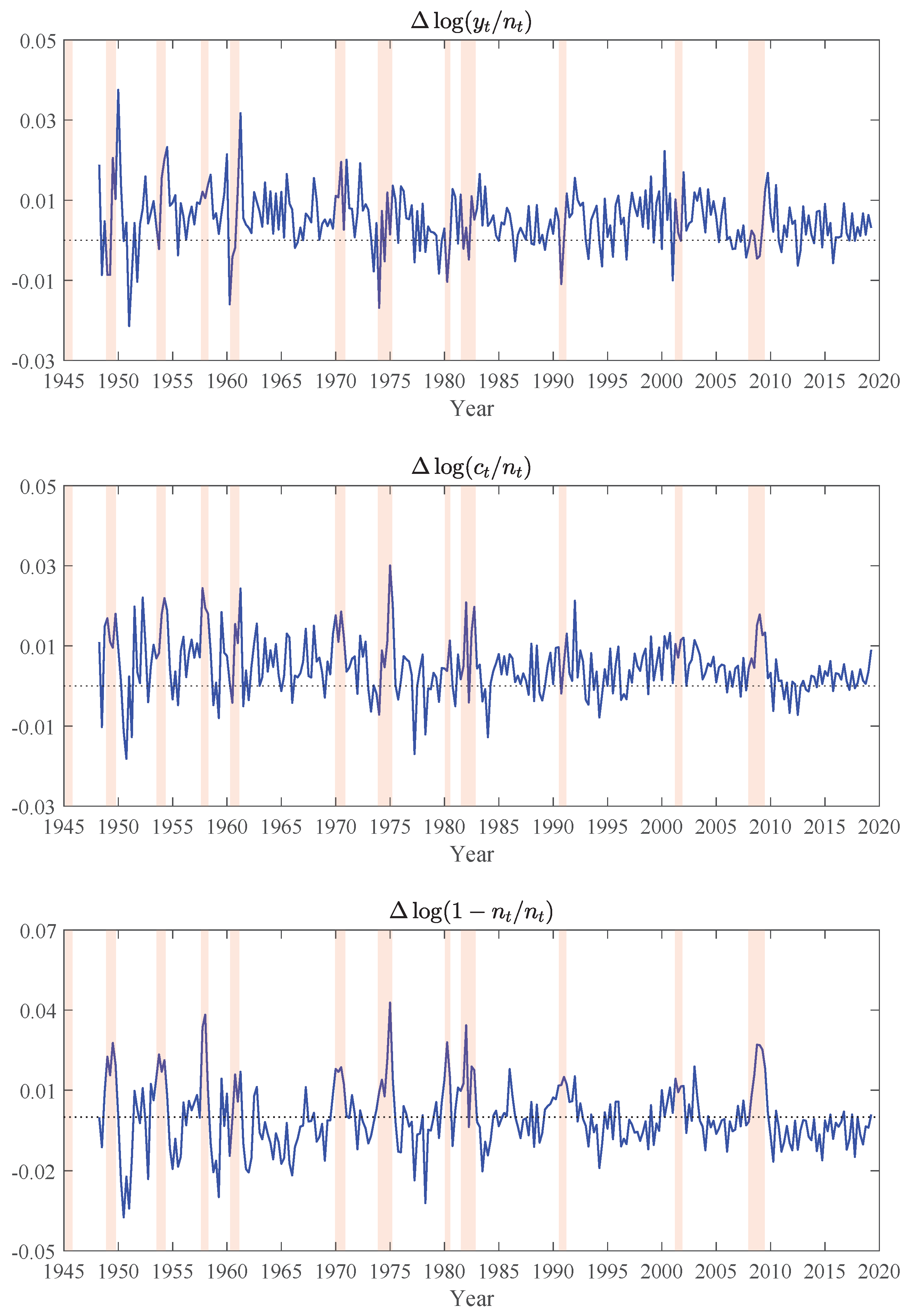
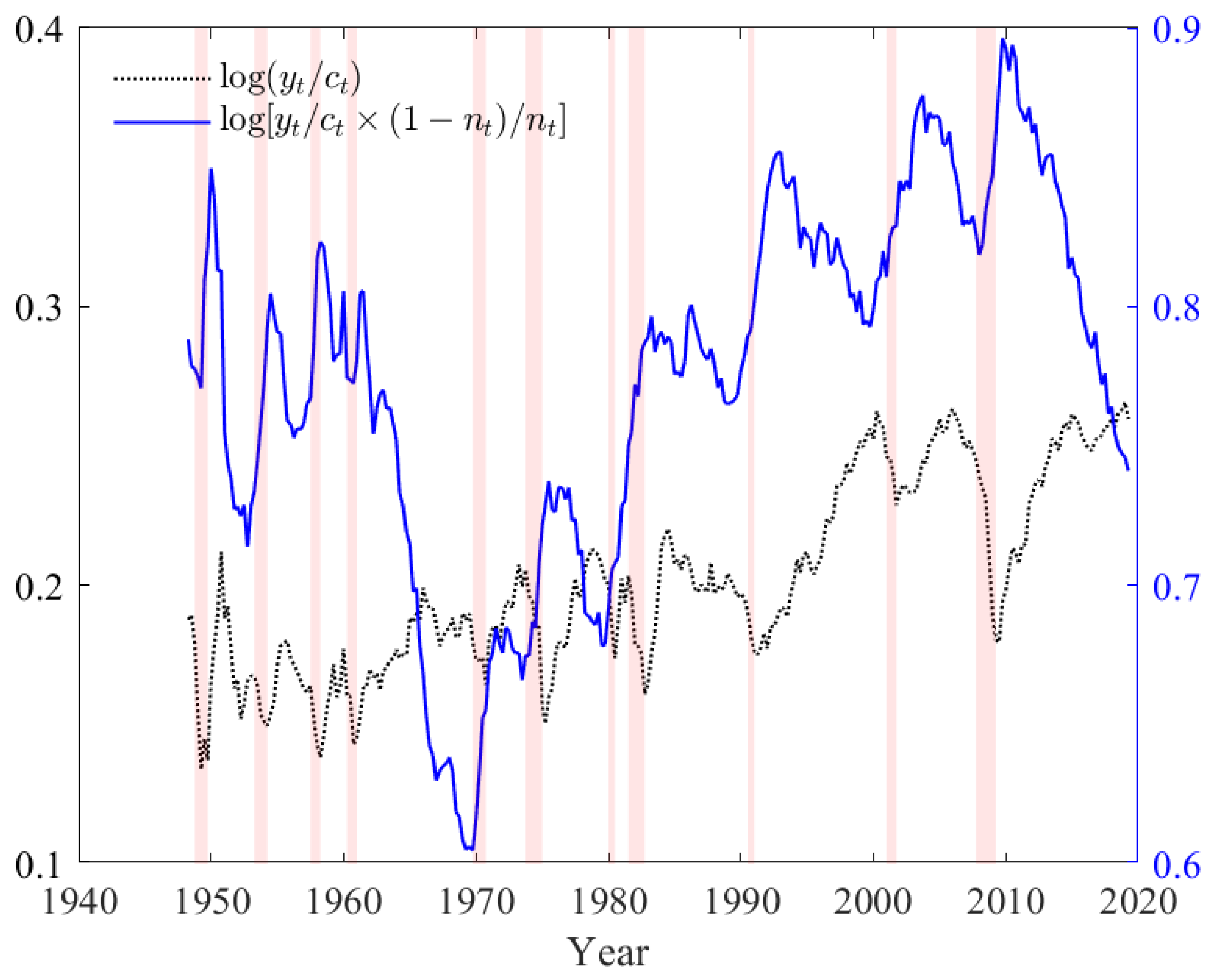
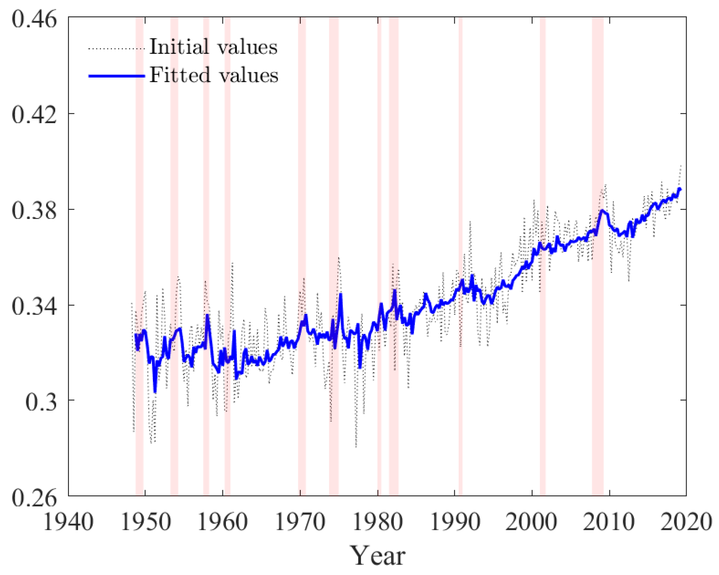
Next, we provide graphical illustrations of the sample values of and from 1948Q1 to 2019Q2 in Figure 1 and Figure 2. It is immediately obvious that the components of , and to a lesser extent, those of are far from being constant over the postwar period. It follows that, since are assumed to be tracking their theoretical counterparts through an ECM process, must themselves have changed considerably over time. Moreover, the pattern of the observed variations suggests that cannot be a function of the sole state variable . Therefore, we need to consider additional state variables (no more than three in order to avoid overfitting). The two natural candidates are and d, as there exists evidence that neither of them has been constant over the postwar period.18 Supporting evidence that the share of capital has been steadily increasing (with cyclical variations) over the postwar period is highlighted in the following quote from Giandrea and Sprague (2017): “In the late 20th century—after many decades of relative stability—the labor share began to decline in the United States and many other economically advanced nations, and in the early 21st century it fell to unprecedented lows.”
Similarly, our estimated state trajectory for (relative preference for consumption versus leisure), as illustrated in Figure 3 below, is broadly comparable with analyses of hours worked in the US. Specifically, Juster and Stafford (1991) document a reduction in hours per week between 1965 and 1981, whereas Jones and Wilson (2018) report a modest increase between 1979 and 2016, resulting from increased women labor participation.
Hence, we adopt the following partition
notwithstanding the fact that it will be ex-post fully validated by the model invariance and recession tracking performance.
As discussed earlier in Section 4.1 the great ratios in Equation (14) initially represent theory derived time-varying cointegration relationships before being transformed into empirically relevant relationships with the introduction of the state vector .20
Next, taking log differences in order to eliminate , we obtain
and
and, by differentiating the second great ratio in in Equation (14), we arrive at
which completes the derivation of the (moving) balanced growth solutions.
Before we proceed to the next section where we discuss recursive estimation of the model, note that the steps that follow are also conditional on a tentative value of , to be calibrated ex-post based upon the recursive validation exercise.
5.2. Recursive Estimation (Conditional on )
Recursive estimation over the validation period , where and proceeds as described in Section 4.2.4 and consists of three steps, to be repeated for any tentative value of , and for all successive values of .
We start the recursive estimation exercise by computing recursive estimates for the state trajectories . First, we estimate as the (recursive) principal component of and for , where this particular choice guarantees consistency with the theory interpretation of from Equations (8), (17) and (18). Next, given estimates of , we rely upon Equation (2) in order to compute estimates of . Therefore, as shown below in Equation (20), the resulting estimates of depend solely on , whereas those of depend on , and , say
for all in .
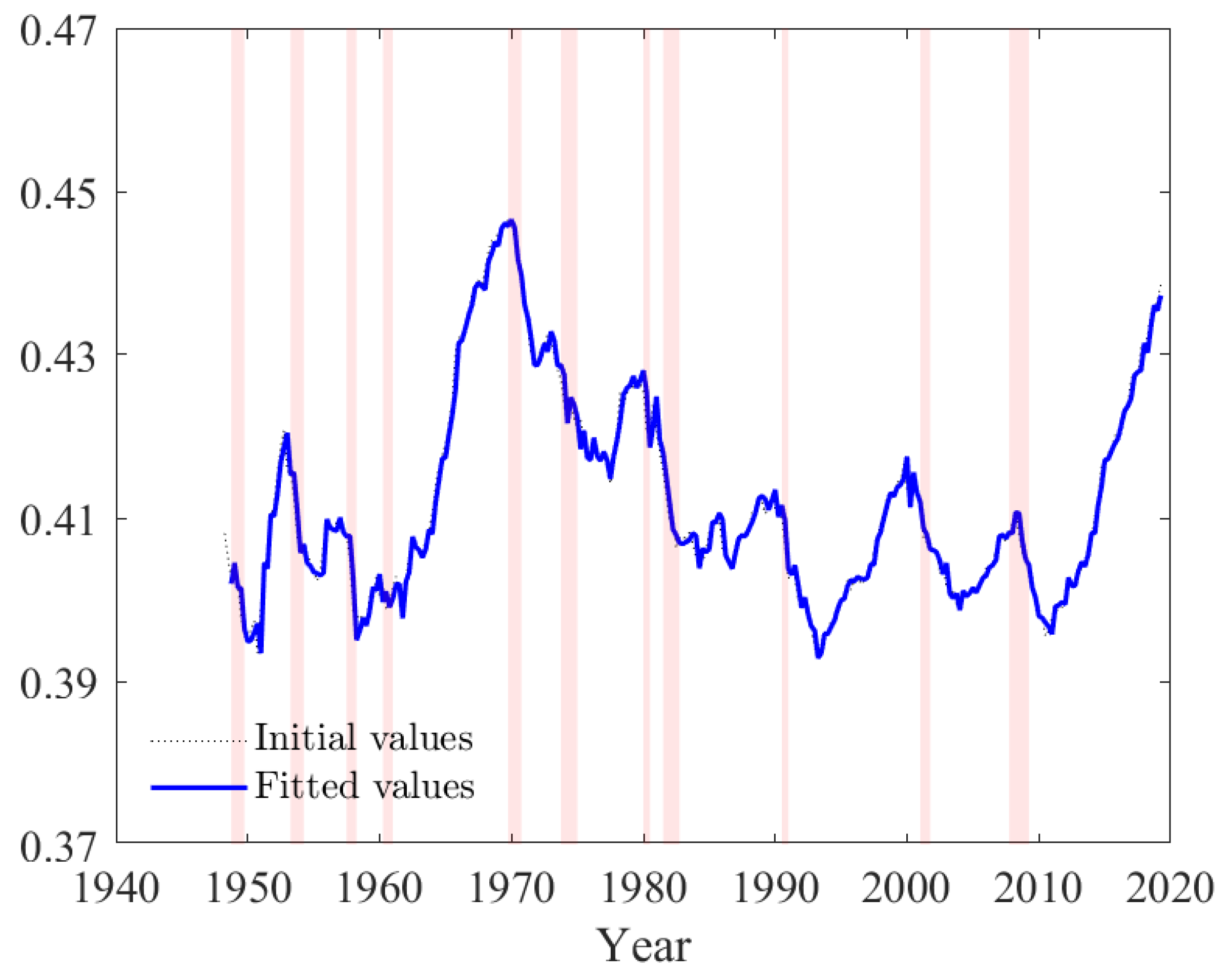
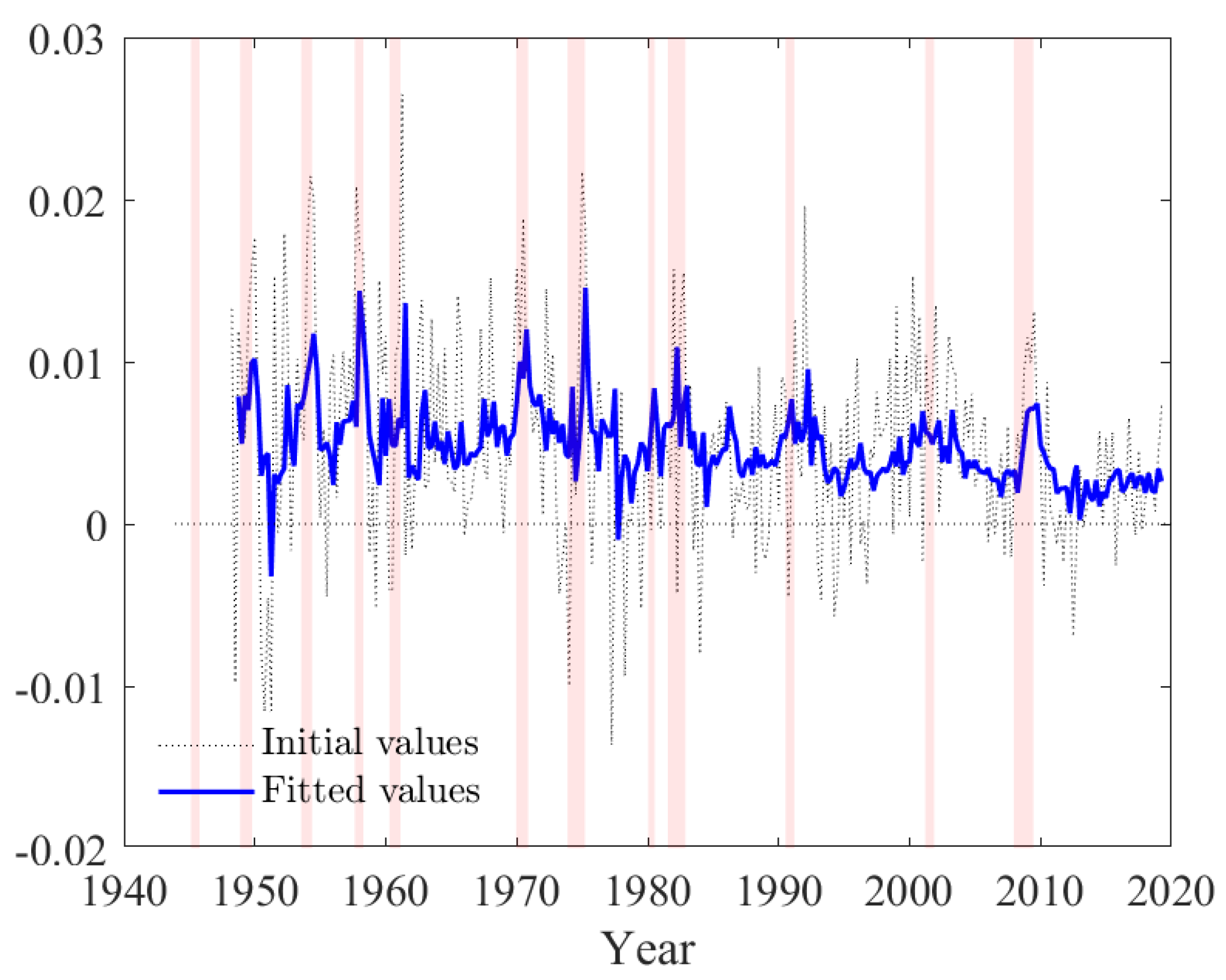
For illustration, we plot the trajectories of for and as dotted lines in Figure 3, Figure 4 and Figure 5, where denotes the calibrated value of , as given further below in Equation (27). The trajectory of highlights a critical feature of the data, which is that typically increases during recessions, and especially during the Great Recession. This apparently surprising feature of the data follows from our theory consistent definition of . Recall that in accordance with Equations (17) and (18), is computed as the principal component of , rather than that of . Hence, the increase of during recessions reflects a common feature of the data which is that typically decreases faster than and during economic downturns. Importantly, this particular behavior proves to be a critical component of the parameter invariance and recession tracking performance of our model, which both outperform those produced when relying instead on the principal component of , which is only theory consistent in equilibrium.
Once we have the trajectories of , our next step is the recursive estimation of the 48 VAR-ECM parameters , where and . The outcome of this recursive exercise (conditional on ) is a full set of recursive estimates given by
Recursive estimates for are obtained using unrestricted OLS, where we find that conditionally on the subsequently calibrated value of , the recursive estimates of are time invariant and statistically significant (though borderline for the intercept). The OLS estimates for and are presented in Table 1 below, whereas the full set of recursive estimates is illustrated in Figure S2 of the Online Supplementary Material.
Recursive OLS estimation of the 27 ECM coefficients in initially produced a majority (19 out of 27) of insignificant coefficients. However, eliminations of insignificant variables has to be assessed not only on the basis of standard test statistics but, also and foremost, on the basis of recursive parameter invariance and recession tracking performance. Hence, we decided to rely upon a sequential system elimination procedure, whereby we sequentially eliminate variables that are insignificant in all three equations, while continuously monitoring the recursive performance of the model.21 This streamline procedure led first to the elimination of the ECM term associated with the great ratio followed by .22 At this stage we were left with seven insignificant coefficients at the two-sided t-test (only three insignificant coefficients at the one-sided t-test). Since the remaining estimates were highly significant in at least one of the system equations, no other variable was removed from the system. The restricted OLS estimates are presented in Table 2, together with t- and F-test statistics. The full set of recursive estimates is illustrated in Figure S3 of the Online Supplementary Material.
At this stage we decided that additional (system or individual) coefficient eliminations were unwarranted. As discussed further below, the recursive performance evaluation of the VAR-ECM model already matches that of the benchmark VAR. Therefore, we have already achieved our main objective with this pilot application which was to demonstrate that under our proposed approach, there no longer is an inherent trade-off between theoretical and empirical coherence and that we can achieve both simultaneously.
5.3. Recursive Tracking/Forecasting (Conditional on )
In this section, we assess the recursive performance of the estimated model conditionally on tentative values of (final calibration of is discussed in Section 5.4 below).
First, for each , we compute fitted values for based upon , , , and . This produces a set of recursive fitted values, say
Similarly and relying upon Monte Carlo (MC) simulations, we produce a full set of recursive i-step ahead out-of-sample point forecasts23
from which we compute mean forecast estimates given by
Since our focus lies on the model’s tracking and forecasting performance in times of rapid changes, we assess the accuracy of the estimates for around the three recessions included in the validation period (1990–91, 2001, and the Great Recession of 2007–09). Specifically, for each recession j we construct a time window consisting of two quarters before recession j, recession j, and six quarters following recession j (as dated by the NBER ), for a total of quarters:24
5.4. Calibration of
The final step of our modeling approach consists of calibrating the time invariant parameters in accordance with the calibration procedure described above in Section 4.2.4.
Estimates of , , and are widely available in the related literature, with and generally tightly estimated in the range, and often loosely identified on a significantly wider interval ranging from 0.1 to 3.0. Searching on those ranges, the calibration of is based upon a combination of informal and formal criteria thought to be critical for accurate recession tracking. The informal criteria consists of the time invariance of the recursive parameter estimates , with special attention paid to the coefficients of the ECM correction term, in Formula (4). The reason for emphasizing this invariance criterion is that tracking and forecasting in the presence of (suspected) structural breaks raises significant complications such as the selection of estimation windows (see for example Pesaran and Timmermann 2007; Pesaran et al. 2006). The formal criteria are the signs of the three non-zero coefficients of the ECM correction term as well as the MAE and RMSE computed for the three recession windows included in the validation period as described in Section 5.3.
The combination of these two sets of criteria led to the following choice of
5.5. Results
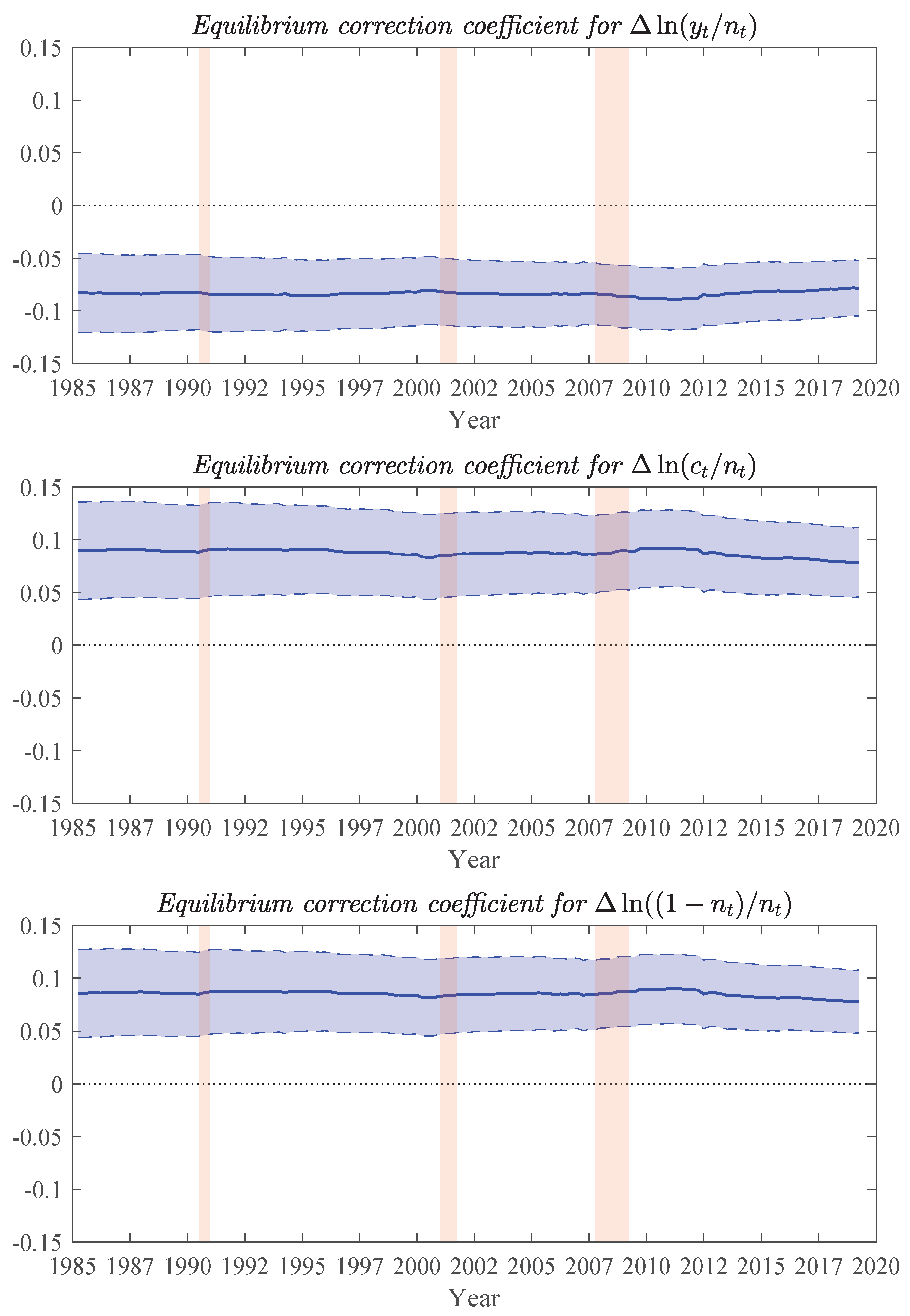
We now discuss the results obtained for our pilot RBC application conditional on the calibrated , given in Equation (27). The first set of results pertain to the invariance of the recursive estimates for ranging from to . In Figure 6, we illustrate the invariance of the three non-zero ECM equilibrium correction coefficients in , together with recursive 95 percent confidence intervals. All three coefficients are statistically significant, time invariant, and with the expected signs suggested by the economic theory: when the great ratio exceeds its target value as defined in Equation (14), the equilibrium corrections are negative for and positive for and —that is negative for .27 Moreover, we find that the quarterly ECM adjustments toward equilibrium are of the order of 8 percent, suggesting a relatively rapid adjustment to the target movements. This is likely a key component in the model quick response to recessions and would guarantee quick convergence to a balanced growth equilibrium were to remain constant for a few years.
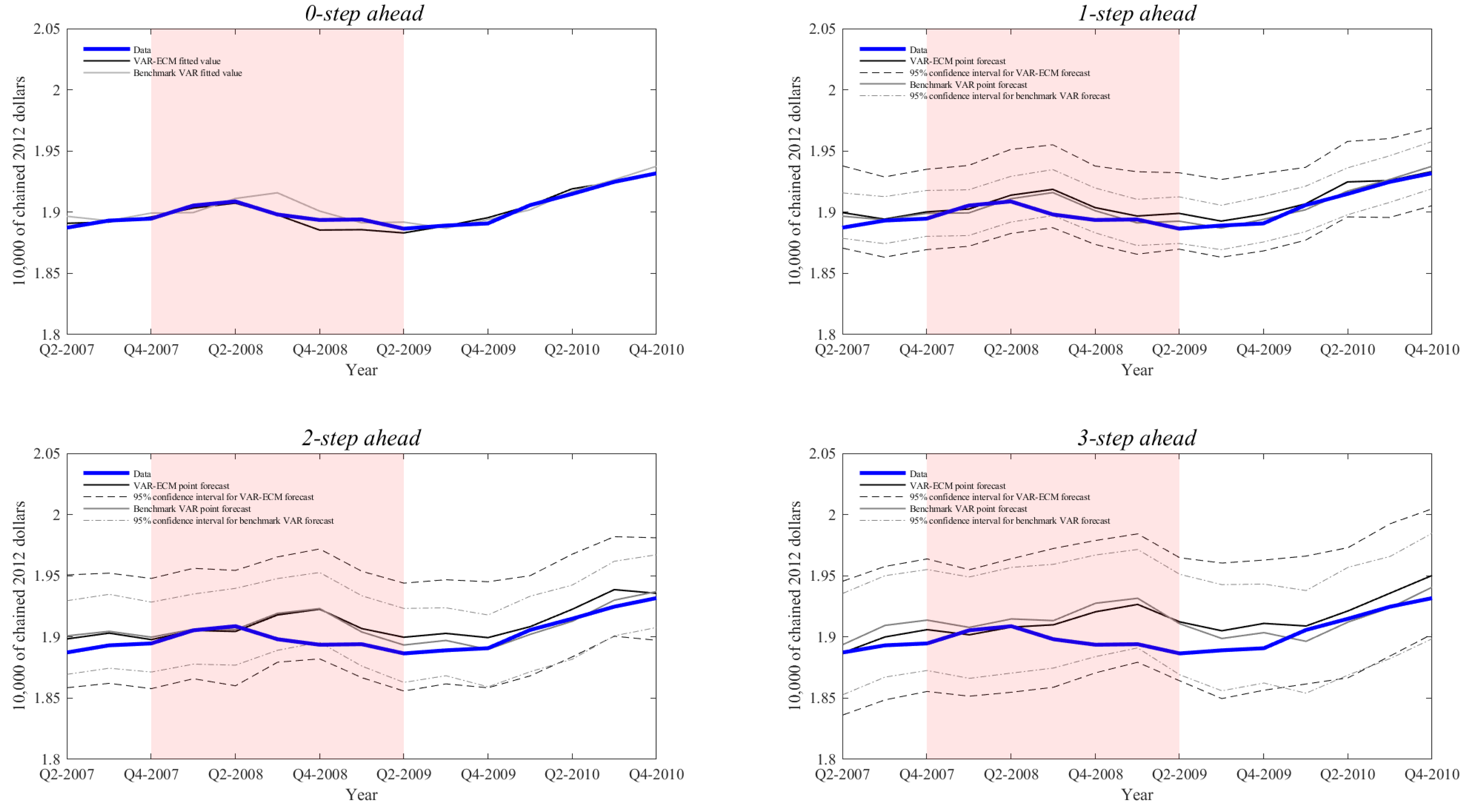
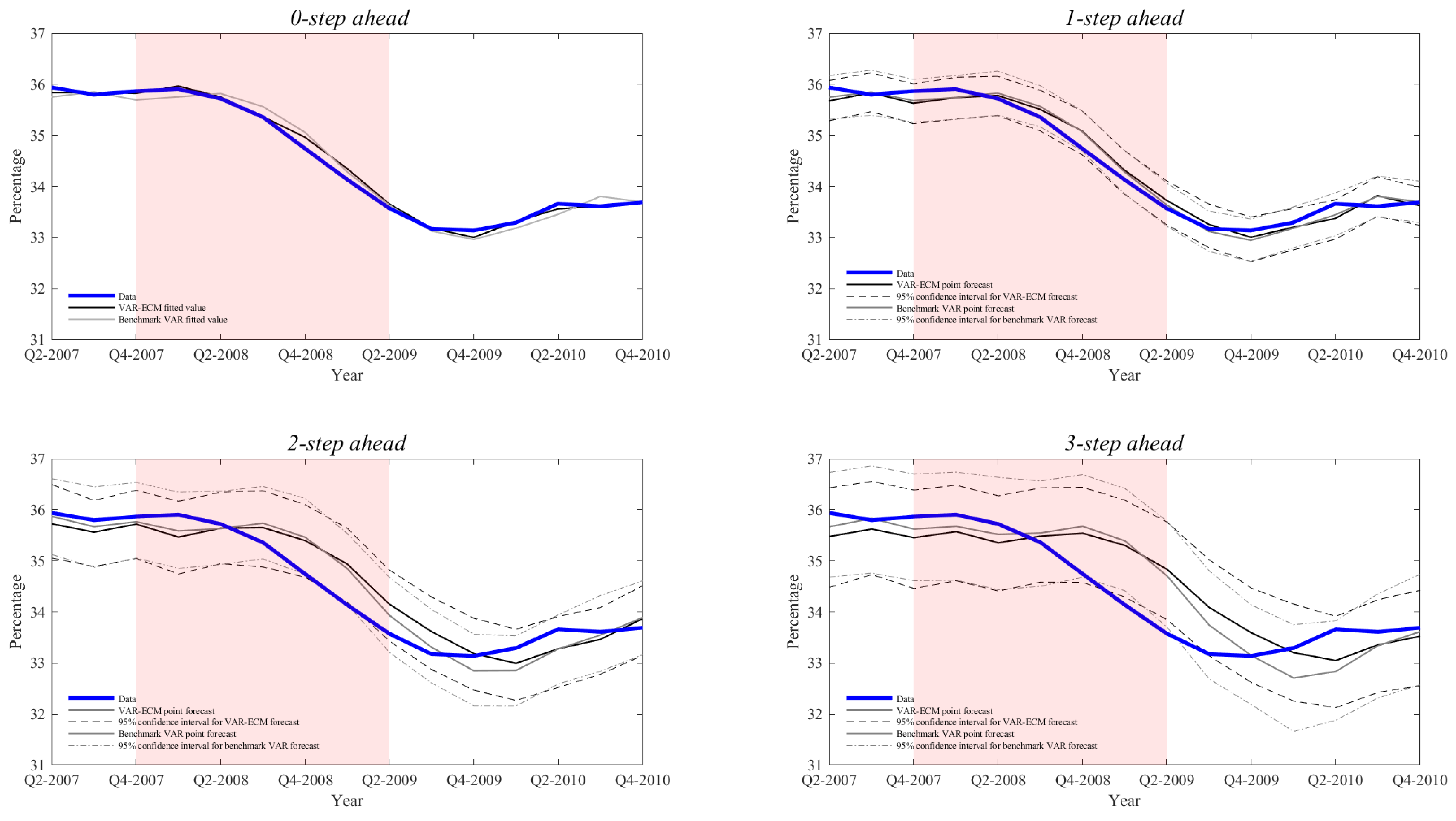
Next, we discuss the tracking and forecasting performance of our hybrid RBC model. In Figure A1, Figure A2 and Figure A3 in Appendix C, we present the Fred data, together with recursive fitted values and 1- to 3-step ahead recursive out-of-sample MC mean forecasts over the time window for the Great Recession.2829 The key message we draw from these figures is that, while both the VAR-ECM and the benchmark VAR track closely the Great Recession and the subsequent economic recovery, they are unable to ex-ante predict its onset and to a lesser extent the subsequent recovery. On a more positive note, we find that the mean forecasts produced by the VAR-ECM outperform those obtained from the benchmark VAR.
For illustration we present summary statistics for the tracking accuracy of the fitted values and the forecasting accuracy of 1- to 3-step ahead mean forecasts for both the VAR-ECM and the VAR benchmark models over the three recession time windows in Table 3. The first two measures under consideration are the MAE and RMSE introduced in Equations (25) and (26), whereas the third metric is the Continuous Rank Probability Score (CRPS) commonly used by professional forecasters to evaluate probabilistic predictions.3031 Based on the MAE and RMSE we find that the VAR-ECM model outperforms the benchmark VAR on virtually all counts (44 out of 48 pairwise comparisons) for the first two recessions, whereas the overall performances of the two models are comparable for the Great Recession (13 out of 24 pairwise comparisons).
The CRPS comparison, on the other hand, is more balanced, reflecting in part the fact that the VAR-ECM forecasts depend on two sources of error ( in the VAR process and in the ECM process), which naturally translates into wider confidence intervals relative to that of the benchmark VAR (14 out of 27 pairwise comparisons).
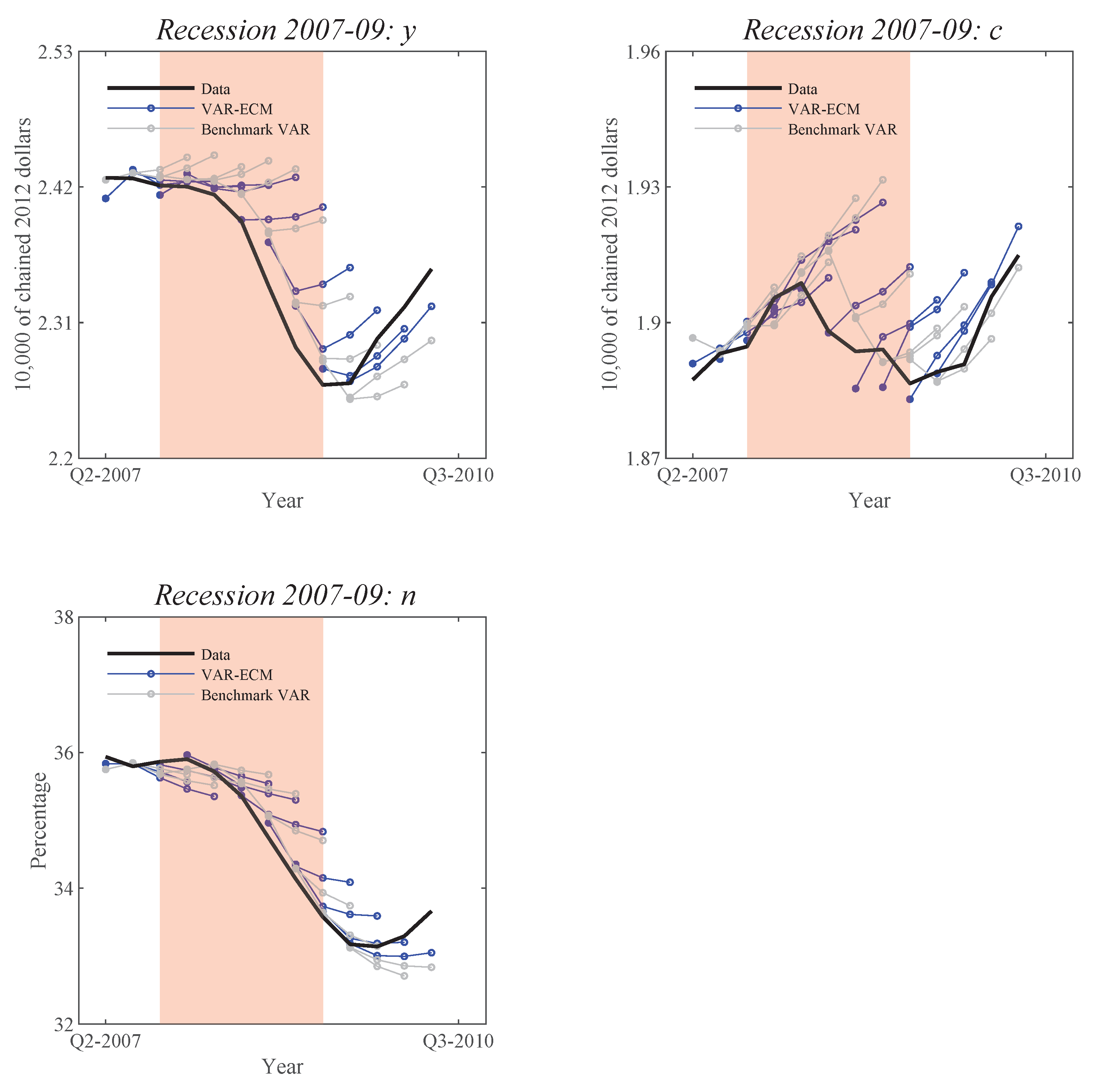
As an alternative way of visualizing these comparisons, we provide in Figure A4 and Figure A5 in the Appendix C take-off versions of hedgehog graphs for the VAR-ECM and benchmark VAR models, where “spine” represents . See Castle et al. (2010) or Ericsson and Martinez (2019) for related images of such graphs and additional details.
5.6. Great Recession and FinancialSeries
Our results indicate that while our RBC model tracks the Great Recession, it fails to ex-ante forecast its onset as the VAR-ECM forecasts respond with a time delay essentially equal to the forecast horizon h. Therefore, a natural question is that of whether we can improve ex-ante forecasting of (the onset of) the Great Recession by incorporating auxiliary macroeconomic aggregates to our baseline RBC model.
As discussed in Section 3, the Great Recession was triggered by the combination of a global financial crisis with the collapse of the housing bubble. This raises the possibility that we might improve ex-ante forecasting by incorporating financial and/or housing variables into the baseline RBC model. However, from an econometric prospective, this approach suffers from three critical limitations.
First and foremost, there exists no precedent to the Great Recession during the postwar period, which inherently limits the possibility of ex-ante estimation of the potential impact of such auxiliary variables. Next, most relevant series have been collected over significantly shorter periods of time than the postwar period for y, c, and n, with start dates mostly from the early sixties to the mid seventies for housing series and from late seventies to mid eighties for financial series. In fact, some of the potentially most relevant series have only been collected from 2007 onward, after their potential relevance for the Great Recession became apparent (for example “Net Percentage of Domestic Banks Reporting Stronger Demand for Subprime Mortgage Loans”). Last but not least, even if it were possible to add financial variables into the model it is unclear whether they would improve the ex-ante forecasting performance since such series are themselves notoriously hard to forecast.
Nevertheless, we decided to analyze whether we might be able to improve the Great Recession ex-ante forecasting performance by incorporating additional variables into our baseline RBC model. First, we selected a total of 20 representative series (10 for the housing sector and 10 for the financial sector) based on their relevance as potential leading indicators to the Great Recession. Second, in order to avoid adding an additional layer of randomness into the VAR-ECM model, we incorporated our auxiliary variables lagged by 4 quarters one at a time as a single additional regressor in the state VAR process.32 Finally, instead of shortening the estimation period as a way of addressing late starting dates of the majority of the auxiliary variables, we set the missing values of the added series equal to zero.33 This approach allows us to provide meaningful comparisons with the results in Table 3, notwithstanding the fact that dramatically shortening the estimation period would inevitably reduce the statistical accuracy, parameter invariance and, foremost, recession tracking performance of the model. The results of this exercise for each of the 20 selected series are presented in Table 4 for the ex-ante forecasting windows in a format comparable to that used in Table 3 for the Great Recession.
Most additions result in deterioration of the forecast accuracy measured by the MAE and RMSE, as one might expect form the incorporation of insignificant variables. The four notable exceptions are the Chicago Fed National Financial Condition Index and three housing variables related to the issuance of building permits, housing starts, and the supply of houses (Housing Starts: New Privately Owned Housing Units Started; New Private Housing Units Authorized by Building Permits; and, to a lesser extent, Monthly Supply of Houses). However, with references to Figure A1, Figure A2 and Figure A3 and Figure A5 in Appendix C, the observed reductions in the corresponding MAE and RMSE do not translate into a mitigation of the delayed responses of ex-ante forecasts.
All together, these results appear to confirm that, as expected, there is a limited scope for structural models to ex-ante forecast recessions as each one has been triggered by unprecedented sets of circumstances. Nevertheless, it remains critical to closely track recessions, as these are precisely times when rapid policy interventions are most critically needed.
We understand that there is much ongoing research aimed at incorporating a financial sector into DSGE models. Twenty years after the Great Recession and accounting for the dramatic impact of the financial crisis, we have no doubts that such efforts will produce models that can better explain how the Great Recession unfolded and, thereby, provide additional policy instruments. However, such ex-post rationalization would not have been possible prior to the recession’s onset. Nor it is likely to improve the ex-ante forecasting of the next recession as there is increasing evidence that it will be triggered by very different circumstances (see Section 3 for a brief discussion on possible triggers of the next US resession).
5.7. Policy Experiment
As we mentioned in the introduction, treating some key structural parameters as time varying state variables allows for state-based policy interventions aimed at mitigating the impact of a recession. Clearly, with a model as simplistic as our pilot RBC model, the scope for realistic policy interventions is very limited. Nevertheless and for illustration purposes, we consider two sets of policy interventions. The first one consists of raising the capital share of output in order to stimulate production in accordance with Equation (8). The other consists of raising the relative importance of consumption versus leisure in Equation (7) or, equivalently lowering d is Equation (10), in order to stimulate consumption.
Keeping in mind that the Cobb-Douglas production function in Equation (8) is highly aggregated to the effect that covers a wide range of industries with very different shares of capital, raising would require shifting production from sectors with low ’s to sectors with high ’s (such as capital intensive infrastructure projects).
As for (or, equivalently, ) in Equation (7) and in the absence of a labor market, low relative preference for consumption versus leisure at this aggregate level covers circumstances that are beyond agents’ control, such as depressed income or involuntarily unemployment. Therefore, one should be able to raise by carefully drafted wages or other employment policies. The combination of the and policies would therefore provide a highly stylized version of the New Deal enacted by F. D. Roosevelt between 1933 and 1939.
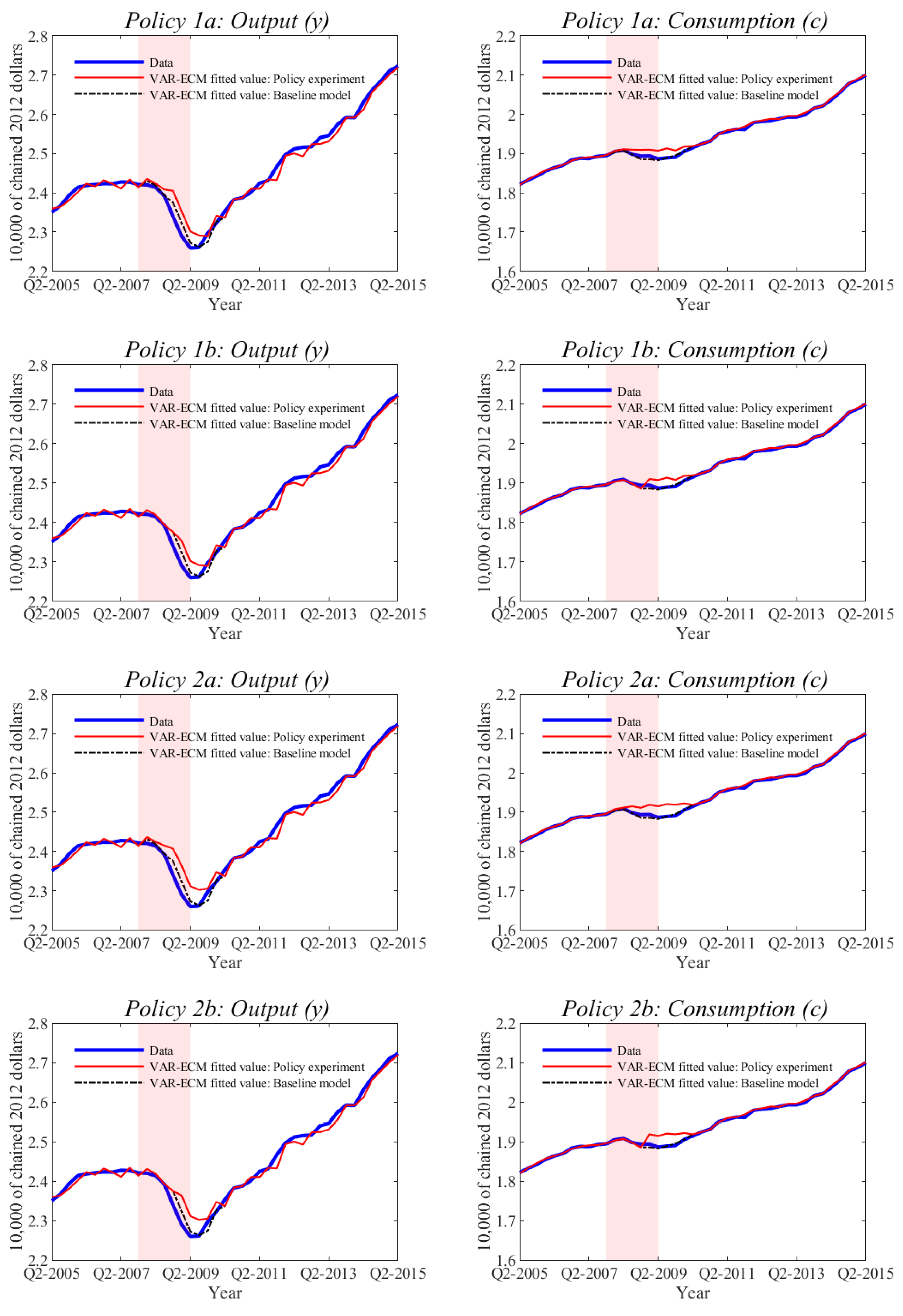
In the present paper, we implement these two artificial policies separately. Since our model fails to ex-ante forecast the onset of the Great Recession but tracks it closely, we consider two versions of each policy: one implemented at the onset of the Great Recession (2007Q4) and the other one delayed by four quarters (2008Q4). The corresponding policies are labeled 1a and 1b for and 2a and 2b for , which is a monotonic transformation of , as defined in Equation (10). All the policies are progressive and last for either five or nine quarters (depending on the policy). This progressive design has the objective of smoothing the transition from the initial impact of a negative shock to the economy until the subsequent recovery. The specific implementation details are illustrated in Table 5 and the results are presented in Figure 7. With reference to Figure 3 and Figure 5, we note that the cumulative sum of the two interventions represent around three times the size of the estimated changes in and from 2007Q4 to 2009Q2. Therefore, and in relation to long-term variations in and , the relative sizes of the two interventions are moderate.
We note that both policies significantly mitigate the impact of the recession on output and consumption. While such conclusion would require deeper analysis in the context of a more realistic model, including in particular a labor market, we find these results to be promising indications of the added policy dimensions resulting from interventions at the level of the additional state variables that would otherwise be treated as constant structural parameters within a conventional DSGE framework. Hence, the results in Figure 7 highlight the potential of (more realistic) implementations of both policies and the importance of their appropriate timing (hence the importance of tracking).
6. Conclusions
We have proposed a generic approach for improving the empirical coherence of structural (DSGE) models with an emphasis on parameter invariance and recession tracking performance while preserving the model’s theoretical coherence.
The key components of our hybrid approach are the use of data that are neither filtered nor detrended, reliance upon (hypothetical) balanced growth solutions interpreted as agents’ theory-derived time-varying cointegrating relationships (moving targets), the use of a state VAR process treating an appropriate subset of structural parameters as state variables, and finally, reliance upon an ECM process to model agents’ responses to their moving targets.
Our application to a pilot RBC model demonstrates the potential of our approach in that it preserves the theoretical coherence of the model and yet matches or even outperforms the empirical performance of an unrestricted VAR benchmark model. Most importantly, our hybrid RBC model closely tracks during the last three postwar recessions, including foremost the 2007–09 Great Recession, a performance largely unmatched by DSGE models and one that is critical for policy interventions at times when they are most needed. In other words, with reference to Pagan (2003) we do not find an inherent trade-off between theoretical and empirical coherence. Our hybrid RBC model achieves both simultaneously.
We also find that, as expected, ex-ante forecasting of recessions is likely to remain econometrically limited using structural models in view of the idiosyncratic nature of recession triggers preventing ex-ante estimation of their potential impact. Hence, the quote from Trichet (2010), as cited in Section 2, remains as relevant as ever. While structural models remain essential for policy analysis and, as we have shown, can match the recession tracking performance of the unrestricted VAR benchmark, they will likely remain inherently limited in their capacity to ex-ante forecast major unexpected shifts. Fortunately, there exists “complementary tools” such as leading indicators, that can bridge that gap.
Last but not least, a potentially promising avenue for future research is one inspired by DeJong et al. (2005), where the authors develop a (reduced form) non-linear model of GDP growth under which regime changes are triggered stochastically by a tension index constructed as a geometric sum of deviations of GDP growth from a sustainable rate. A quick look at Figure 4 and Figure 5 suggests that a similar index could be derived from the state variables, where the key issue would be that of incorporating such a trigger within the VAR component of our hybrid model.
Supplementary Materials
The following are available online at https://0-www-mdpi-com.brum.beds.ac.uk/2225-1146/8/2/14/s1, Figure S1: Data used in the estimation of the RBC pilot model; Figure S2: VAR-ECM model: VAR recursive parameter estimates; Figure S3: VAR-ECM model: ECM recursive parameter estimates; Figure S4: Benchmark VAR model: VAR recursive parameter estimates; Figure S5: Recursive fitted values for real output per capita; Figure S6: Recursive fitted values for real output per capita; Figure S7: Recursive fitted values for the fraction of time spent working; Figure S8: Out-of-sample 1-step ahead recursive forecasts for real output per capita; Figure S9: Out-of-sample 1-step ahead recursive forecasts for real consumption per capita; Figure S10: Out-of-sample 1-step ahead recursive forecasts for the fraction of time spent working; Figure S11: Out-of-sample 2-step ahead recursive forecasts for real output per capita; Figure S12: Out-of-sample 2-step ahead recursive forecasts for real consumption per capita; Figure S13: Out-of-sample 2-step ahead recursive forecasts for the fraction of time spent working; Figure S14: Out-of-sample 3-step ahead recursive forecasts for real output per capita; Figure S15: Out-of-sample 3-step ahead recursive forecasts for real consumption per capita; Figure S16: Out-of-sample 3-step ahead recursive forecasts for the fraction of time spent working; Figure S17: Recession of 1990–91: Out-of-sample 0-to-3-step ahead recursive forecasts for real output per capita; Figure S18: Recession of 1990–91: Out-of-sample 0-to-3-step ahead recursive forecasts for real consumption per capita; Figure S19: Recession of 1990–91: Out-of-sample 0-to-3-step ahead recursive forecasts for the fraction of time spent working; Figure S20: Recession of 2001: Out-of-sample 0-to-3-step ahead recursive forecasts for real output per capita; Figure S21: Recession of 2001: Out-of-sample 0-to-3-step ahead recursive forecasts for real consumption per capita; Figure S22: Recession of 2001: Out-of-sample 0-to-3-step ahead recursive forecasts for the fraction of time spent working.
Author Contributions
Both authors are full contributors to the paper. All authors have read and agreed to the published version of the manuscript.
Funding
We gratefully acknowledge support provided by the National Science Foundation under grant SES-1529151.
Acknowledgments
For helpful comments, we thank Stefania Albanesi, David DeJong, guest editor Neil Ericsson, David Hendry, Sewon Hur, Roman Liesenfeld, Marla Ripoll, and participants at the Conference on Growth and Business Cycles in Theory (University of Manchester), the Midwest Macro Meetings (Vanderbilt University), and the QMUL Economics and Finance Workshop (Queen Mary University of London). Moreover, we are very grateful to the three anonymous referees for their insightful comments and helpful suggestions.
Conflicts of Interest
The authors declare no conflicts of interest.
Appendix A. Data

Table A1.
Fred data series.
| Fred Series Name and Identification Code | Units and Seasonal Adjustment | Frequency | Range |
|---|---|---|---|
| Real Personal Consumption Expenditures: Services (DSERRA3Q086SBEA) | Index 2012=100, SA | Quarterly | 1948Q1–2019Q2 |
| Real Personal Consumption Expenditures: Services (PCESVC96) | Billions of chained 2012 dollars, SAAR | Quarterly | 2002Q1–2019Q2 |
| Real Personal Consumption Expenditures: Nondurable Goods (DNDGRA3Q086SBEA) | Index 2012=100, SA | Quarterly | 1948Q1–2019Q2 |
| Real Personal Consumption Expenditures: Nondurable Goods (PCNDGC96) | Billions of chained 2012 dollars, SAAR | Quarterly | 2002Q1–2019Q2 |
| Real Gross Private Domestic Investment | Billions of chained 2012 dollars, SAAR | Quarterly | 1948Q1–2019Q2 |
| (GPDIC1) | |||
| Civilian Noninstitutional Population: 25 to 54 Years (LNU00000060) | Thousands of persons, NSA | Quarterly | 1948Q1–2019Q2 |
SA denotes seasonally adjusted, NSA not seasonally adjusted, and SAAR seasonally adjusted annual rate.
Appendix A.1. Consumption
We construct the quarterly seasonally-adjusted data on real consumption per capita () by dividing the sum of real consumption expenditures in services () and non-durable goods () by the working-age population ()
where the division by 4 accounts for the annualization of the original Fred series on consumption.
The resulting is measured in billions of chained 2012 dollars (see middle panel of Figure S1 of the Online Supplementary Material).
Appendix A.2. Output
Similarly, we construct quarterly seasonally-adjusted data on on real output per capita () by dividing the sum of real consumption expenditures (in services and non-durable goods) and real gross private domestic investments () by the working-age population
where again the division by 4 accounts for the annualization of the original Fred series on both consumption and investments.
The resulting is measured in billions of chained 2012 dollars (see top panel of Figure S1 of the Online Supplementary Material).
Appendix A.3. Fraction of Time Spent Working
Finally, we compute the fraction of time spent working () by dividing total hours worked in the US economy () by the working-age population and , assuming a daily average of 16 h of a discretionary time
where the data on total hours worked comes from the Office of Productivity and Technology of the U.S. Bureau of Labor Statistics.
The resulting belongs to the interval (see bottom panel of Figure S1 of the Online Supplementary Material).
Appendix B. Pseudo Code for the RBC Application
Structural time invariant parameters: . State variables: .
Observables: . t goes from 1948Q1 to 2019Q2, where .
- Set .
- Start calibration loop:
- 2.1.
- Select .
- Start recursive loop (given ):
- 3.1.
- Set .
- 3.2.
- Estimate state variables:Set to a principal component of and , .Given optimize in :where .
- 3.3.
- Estimate the VAR process for :where .Store and .
- 3.4.
- Estimate the ECM process for :where , andStore and .
- 3.5.
- Compute fitted values .
- 3.6.
- Conduct MC forecast simulation :
- 3.6.1.
- Forecast 1- to 3-step ahead from VAR: .
- 3.6.2.
- Forecast 1- to 3-step ahead from ECM: given .
- 3.6.3.
- Recover and store .
- If , then and go to 3.2. Else, end recursive loop.
- Evaluate recursive performance. For :
- 5.1.
- Graph and .
- 5.2.
- Compute mean 1- to 3-step ahead forecasts: , .
- 5.3.
- Graph fitted values and 1- to 3-step ahead mean forecasts .
- 5.4.
- Graph MC 95 percent confidence intervals for .
- 5.5.
- Compute the MAE and RMSE for , for , .
- As needed, return to 2.1 and select a different value of .
Appendix C. Additional Figures
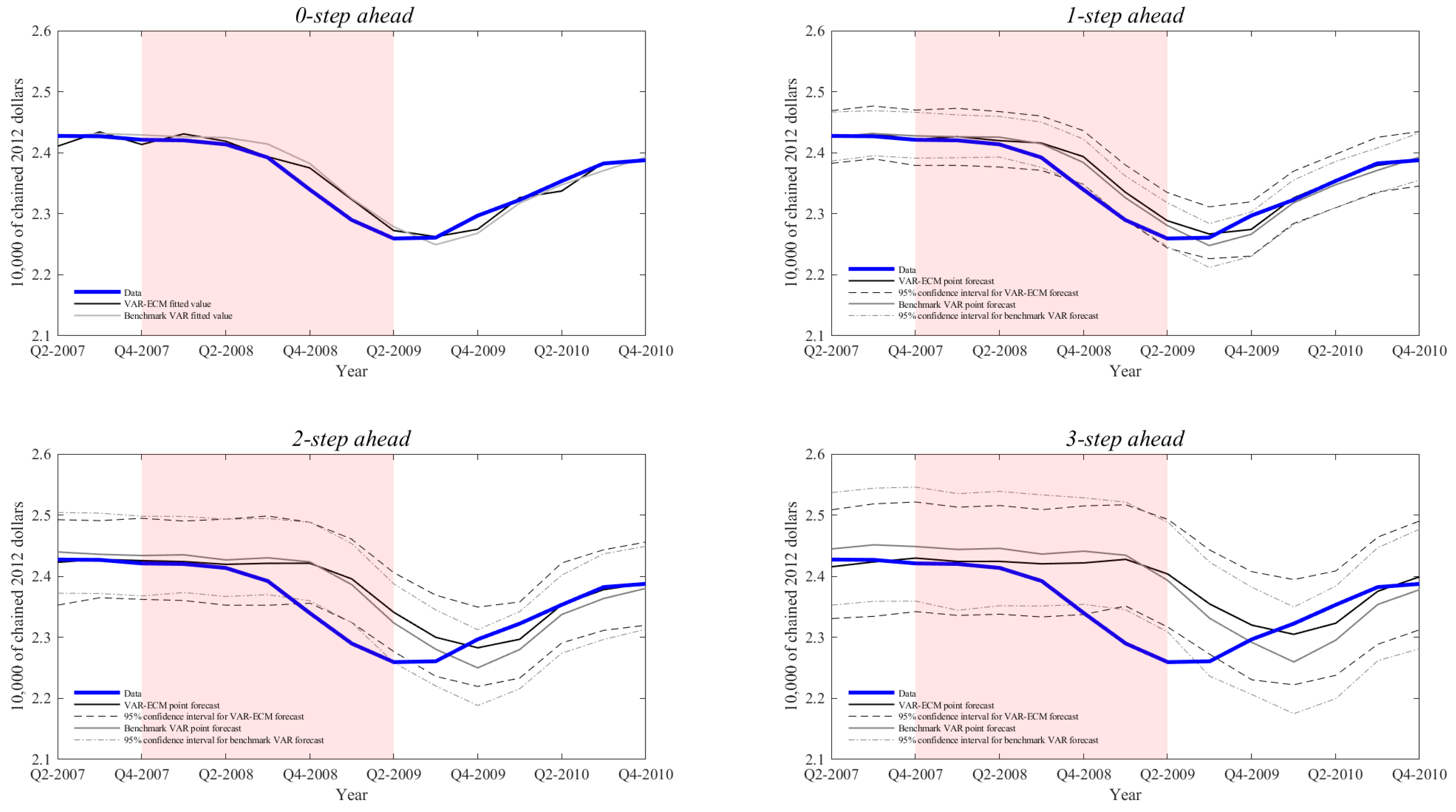
Figure A1.
Recession of 2007–2009: Out-of-sample 0- to 3-step ahead recursive forecasts for real output per capita. In the top left figure, the solid thin lines correspond to fitted values. In the remaining figures, the solid thin lines denote the mean forecasts calculated over 1000 MC repetitions and the dashed lines the corresponding 95 percent confidence intervals. In all figures the solid thick line denotes the Fred data. Shaded regions correspond to NBER recession dates.

Figure A2.
Recession of 2007–09: Out-of-sample 0- to 3-step ahead recursive forecasts for real consumption per capita. In the top left figure, the solid thin lines correspond to fitted values. In the remaining figures, the solid thin lines denote the mean forecasts calculated over 1,000 MC repetitions and the dashed lines the corresponding 95 percent confidence intervals. In all figures the solid thick line denotes the Fred data. Shaded regions correspond to NBER recession dates.

Figure A3.
Recession of 2007–09: Out-of-sample 0- to 3-step ahead recursive forecasts for the fraction of time spent working. In the top left figure, the solid thin lines correspond to fitted values. In the remaining figures, the solid thin lines denote the mean forecasts calculated over 1000 MC repetitions and the dashed lines the corresponding 95 percent confidence intervals. In all figures the solid thick line denotes the Fred data. Shaded regions correspond to NBER recession dates.

Figure A4.
Hedgehog graphs for 0- to 3-step ahead forecasts for y, c, and n around the 1990–91 and 2001 recessions. Shaded regions correspond to NBER recession dates. Filled circles denote tracked values and empty circles 1- to 3-step ahead forecasts.
Figure A4.
Hedgehog graphs for 0- to 3-step ahead forecasts for y, c, and n around the 1990–91 and 2001 recessions. Shaded regions correspond to NBER recession dates. Filled circles denote tracked values and empty circles 1- to 3-step ahead forecasts.

Figure A5.
Hedgehog graphs for 0- to 3-step ahead forecasts for y, c, and n around the 2007-09 Great Recession. Shaded regions correspond to NBER recession dates. Filled circles denote tracked values and empty circles 1- to 3-step ahead forecasts.
Figure A5.
Hedgehog graphs for 0- to 3-step ahead forecasts for y, c, and n around the 2007-09 Great Recession. Shaded regions correspond to NBER recession dates. Filled circles denote tracked values and empty circles 1- to 3-step ahead forecasts.

References
- An, Sungbae, and Frank Schorfheide. 2007. Bayesian analysis of DSGE models. Econometric Review 26: 113–72. [Google Scholar] [CrossRef] [Green Version]
- Bierens, Herman J., and Luis F. Martins. 2010. Time-varying cointegration. Econometric Theory 26: 1453–90. [Google Scholar] [CrossRef] [Green Version]
- Blanchard, Olivier. 2016. Do DSGE models have a future? In Policy Brief. Washington, DC: Peterson Institute for International Economics, pp. 16–11. [Google Scholar]
- Caballero, Ricardo J. 2010. Macroeconomics after the crisis: Time to deal with the pretense-of-knowledge syndrome. Journal of Economic Perspectives 24: 85–102. [Google Scholar] [CrossRef] [Green Version]
- Canova, Fabio, and Fernando J. Pérez Forero. 2015. Estimating overidentified, nonrecursive, time-varying coefficients structural vector autoregressions. Quantitative Economics 6: 359–84. [Google Scholar] [CrossRef] [Green Version]
- Cardinali, Alessandro, and Guy P. Nason. 2010. Costationarity of locally stationary time series. Journal of Time Series Econometrics 2: 1–33. [Google Scholar] [CrossRef]
- Carroll, Christopher D. 2000. Saving and growth with habit formation. American Economic Review 90: 341–55. [Google Scholar] [CrossRef]
- Castle, Jennifer L., Michael P. Clements, and David F. Hendry. 2016. An overview of forecasting facing breaks. Journal of Business Cycle Research 12: 3–23. [Google Scholar] [CrossRef] [Green Version]
- Castle, Jennifer L., Nicholas W. P. Fawcett, and David F. Hendry. 2010. Forecasting with equilibrium-correction models during structural breaks. Journal of Econometrics 158: 25–36. [Google Scholar] [CrossRef] [Green Version]
- Chari, V. V., Patrick J. Kehoe, and Ellen R. McGrattan. 2007. Business cycle accounting. Econometrica 75: 781–836. [Google Scholar] [CrossRef] [Green Version]
- Chari, V. V., Patrick J. Kehoe, and Ellen R. McGrattan. 2009. New Keynesian models: Not yet useful for policy analysis. American Economic Journal: Macroeconomics 1: 242–66. [Google Scholar] [CrossRef] [Green Version]
- Christiano, Lawrence J., and Joshua M. Davis. 2006. Two Flaws in Business Cycle Accounting. NBER Working Papers 12647. Cambridge: National Bureau of Economic Research. [Google Scholar]
- Christiano, Lawrence J., Martin S. Eichenbaum, and Mathias Trabandt. 2018. On DSGE models. Journal of Economic Perspectives 32: 113–40. [Google Scholar] [CrossRef] [Green Version]
- Clements, Michael P., and David F. Hendry. 1993. On the limitations of comparing mean square forecast errors. Journal of Forecasting 12: 617–37. [Google Scholar] [CrossRef]
- Deaton, Angus. 1991. Saving and liquidity constraints. Econometrica 59: 1221–48. [Google Scholar] [CrossRef]
- Del Negro, Marco, and Frank Schorfheide. 2008. Forming priors for DSGE models (and how it affects the assessment of nominal rigidities). Journal of Monetary Economics 55: 1191–208. [Google Scholar] [CrossRef] [Green Version]
- DeJong, David N., and Chetan Dave. 2011. Structural Macroeconomics, 2nd ed. Princeton: Princeton University Press. [Google Scholar]
- DeJong, David N., Roman Liesenfeld, Guilherme V. Moura, Jean-François Richard, and Hariharan Dharmarajan. 2013. Efficient likelihood evaluation of state-space representations. Review of Economic Studies 80: 538–67. [Google Scholar] [CrossRef]
- DeJong, David N., Roman Liesenfeld, and Jean-François Richard. 2005. A nonlinear forecasting model of GDP growth. The Review of Economics and Statistics 87: 697–708. [Google Scholar] [CrossRef]
- Elliott, Graham, and Allan Timmermann. 2016. Forecasting in economics and finance. Annual Review of Economics 8: 81–110. [Google Scholar] [CrossRef] [Green Version]
- Ericsson, Neil R., and Andrew B. Martinez. 2019. Evaluating government budget forecasts. In The Palgrave Handbook of Government Budget Forecasting. Edited by D. Williams and T. Calabrese. Cham: Palgrave Macmillan. [Google Scholar]
- Giandrea, Michael D., and Shawn Sprague. 2017. Estimating the U.S. Labor Share. Monthly Labor Review. U.S. Bureau of Labor Statistics: Available online: https://0-doi-org.brum.beds.ac.uk/10.21916/mlr.2017.7 (accessed on 12 August 2019).
- Grimit, Eric P., Tilmann Gneiting, Veronica J. Berrocal, and Nicholas A. Johnson. 2006. The continuous ranked probability score for circular variables and its application to mesoscale forecast ensemble verification. Quarterly Journal of the Royal Meteorological Society 132: 2925–42. [Google Scholar] [CrossRef] [Green Version]
- Hamilton, James D. 2018. Why you should never use the Hodrick-Prescott filter. Review of Economics and Statistics 100: 831–43. [Google Scholar] [CrossRef]
- Hendry, David F., and Grayham E. Mizon. 1993. Evaluating dynamic econometric models by encompassing the VAR. In Models, Methods and Applications of Econometrics. Edited by P. C. B. Phillips. Cambridge: Blackwell. [Google Scholar]
- Hendry, David F., and Grayham E. Mizon. 2014a. Unpredictability in economic analysis, econometric modeling and forecasting. Journal of Econometrics 182: 186–95. [Google Scholar] [CrossRef] [Green Version]
- Hendry, David F., and Grayham E. Mizon. 2014b. Why DSGEs crash during crises. VOX CEPR’s Policy Portal. Available online: https://voxeu.org/article/why-standard-macro-models-fail-crises (accessed on 12 August 2009).
- Hendry, David F., and John N. J. Muellbauer. 2018. The future of macroeconomics: Macro theory and models at the Bank of England. Oxford Review of Economic Policy 34: 287–328. [Google Scholar] [CrossRef]
- Hendry, David F., and Jean-François Richard. 1982. On the formulation of empirical models in dynamic econometrics. Journal of Econometrics 20: 3–33. [Google Scholar] [CrossRef]
- Hendry, David F., and Jean-François Richard. 1989. Recent developments in the theory of encompassing. In Contributions to Operation Research and Econometrics: The Twentieth Anniversary of CORE. Edited by B. Cornet and H. Tulkens. Cambridge: MIT press. [Google Scholar]
- Ingram, Beth F., and Charles H. Whiteman. 1994. Supplanting the ’Minnesota’ prior: Forecasting macroeconomic time series using real business cycle model priors. Journal of Monetary Economics 34: 497–510. [Google Scholar] [CrossRef]
- Jones, Janelle, and Valerie Wilson. 2018. Working Harder or Finding It Harder to Work: Demographic Trneds in Annual Work Hours Show an Increasingly Featured Workforce. Washington, DC: Economic Policy Institute. [Google Scholar]
- Jusélius, Katarina, and Massimo Franchi. 2007. Taking a DSGE model to the data meaningfully. Economics-ejournal 1: 1–38. [Google Scholar] [CrossRef] [Green Version]
- Juster, Thomas F., and Frank P. Stafford. 1991. The allocation of time: Empirical findings, behavioral models, and problems of measurement. Journal of Economic Literature 29: 471–522. [Google Scholar]
- Korinek, Anton. 2017. Thoughts on DSGE Macroeconomics: Matching the Moment, but Missing the Point? Paper presented at the 2015 Festschrift Conference ’A Just Society’ Honoring Joseph Stiglitz’s 50 Years of Teaching; Available online: https://papers.ssrn.com/sol3/papers.cfm?abstract_id=3022009 (accessed on 29 August 2019).
- Matteson, David S., Nicholas A. James, William B. Nicholson, and Louis C. Segalini. 2013. Locally Stationary Vector Processes and Adaptive Multivariate Modeling. Paper presented at the 2013 IEEE International Conference on Acoustics, Speech and Signal Processing, Vancouver, BC, Canada, May 26–31; pp. 8722–26. [Google Scholar]
- Mizon, Grayham E., and Jean-François Richard. 1986. The encompassing principle and its application to testing non-nested hypotheses. Econometrica 54: 657–78. [Google Scholar] [CrossRef]
- Mizon, Grayham E. 1984. The encompassing approach in econometrics. In Econometrics and Quantitative Economics. Edited by D. F. Hendry and K. F. Wallis. Oxford: Blackwell. [Google Scholar]
- Muellbauer, John N. J. 2016. Macroeconomics and consumption: Why central bank models failed and how to repair them. VOX CEPR’s Policy Portal. Available online: https://voxeu.org/article/why-central-bank-models-failed-and-how-repair-them (accessed on 15 February 2019).
- Pagan, Adrian. 2003. Report on Modelling and Forecasting at the Bank of England. Quarterly Bulletin. London: Bank of England. [Google Scholar]
- Pesaran, M. Hashem, and Allan Timmermann. 2007. Selection of estimation window in the presence of breaks. Journal of Econometrics 137: 134–61. [Google Scholar] [CrossRef]
- Pesaran, M. Hashem, Davide Pettenuzzo, and Allan Timmermann. 2006. Forecasting time series subject to multiple structural breaks. Review of Economic Studies 73: 1057–84. [Google Scholar] [CrossRef]
- Romer, Paul. 2016. The trouble with macroeconomics. The American Economist. Forthcoming. [Google Scholar]
- Rubio-Ramírez, Juan F., and Jesús Fernández-Villaverde. 2005. Estimating dynamic equilibrium economies: Linear versus nonlinear likelihood. Journal of Applied Econometrics 20: 891–910. [Google Scholar]
- Schorfheide, Frank. 2011. Estimation and Evaluation of DSGE Models: Progress and Challenges. NBER Working Papers 16781. Cambridge: National Bureau of Economic Research. [Google Scholar]
- Sims, Christopher A. 2007. Monetary Policy Models. CEPS Working Papers 155. Brussels: CEPS. [Google Scholar]
- Smets, Frank, and Raf Wouters. 2005. Comparing shocks and frictions in US and Euro area business cycles: A Bayesian DSGE approach. Journal of Applied Econometrics 20: 161–83. [Google Scholar] [CrossRef] [Green Version]
- Smets, Frank, and Raf Wouters. 2007. Shocks and frictions in US business cycles: A Bayesian DSGE approach. American Economic Review 97: 586–606. [Google Scholar] [CrossRef] [Green Version]
- Stiglitz, Joseph E. 2018. Where modern macroeconomics went wrong. Oxford Review of Economic Policy 34: 70–106. [Google Scholar] [CrossRef]
- Trichet, Jean-Claude. 2010. Reflections on the nature of monetary policy non-standard measures and finance theory. Opening address at the ECB Central Banking Conference, Frankfurt, Germany, November 18. [Google Scholar]
- Wallis, Kenneth F. 1974. Seasonal adjustment and relations between variables. Journal of the American Statistical Association 69: 18–31. [Google Scholar] [CrossRef]
- Wieland, Volker, and Maik Wolters. 2012. Macroeconomic model comparisons and forecast competitions. VOX CEPR’s Policy Portal. Available online: https://voxeu.org/article/failed-forecasts-and-financial-crisis-how-resurrect-economic-modelling (accessed on 15 January 2019).
| 1. | |
| 2. | It follows that the ECM parsimounsly encompasses the initial VAR model. See Hendry and Richard (1982, 1989); Mizon and Richard (1986); Mizon (1984) for a discussion of the concept of encompassing and its relevance for econometric models. |
| 3. | See also An and Schorfheide (2007) for a survey of Bayesian methods used to evaluate DSGE models and an extensive list of related references. |
| 4. | In the present paper, we follow Pagan (2003) by using an unrestricted VAR as a standard benchmark to assess the empirical relevance of our proposed model. Potential extensions to Bayesian VARs belong to future research (though imposing a DSGE-type prior density on VAR in order to improve its theoretical relevance could negatively impact its empirical performance). |
| 5. | A similar message was delivered by Jerome Powell in his swearing-in ceremony as the new Chair of the Federal Reserve: “The success of our institution is really the result of the way all of us carry out our responsibilities. We approach every issue through a rigorous evaluation of the facts, theory, empirical analysis and relevant research. We consider a range of external and internal views; our unique institutional structure, with a Board of Governors in Washington and 12 Reserve Banks around the country, ensures that we will have a diversity of perspectives at all times. We explain our actions to the public. We listen to feedback and give serious consideration to the possibility that we might be getting something wrong. There is great value in having thoughtful, well-informed critics”. (See https://www.federalreserve.gov/newsevents/speech/powell20180213a.htm for the complete speech given during the ceremonial swearing-in on February 13, 2018). |
| 6. | For more details see https://www.youtube.com/watch?v=lyzS7Vp5vaY (Stiglitz’s interview posted on May 6, 2019) and https://www.youtube.com/watch?v=rUYk2DA8PH8 (Schiller’s interview posted on April 1, 2019). |
| 7. | For the full article see https://www.theguardian.com/business/2019/feb/05/financial-crisis-us-uk-crash. February, 2019. |
| 8. | By doing so, we avoid producing “series with spurious dynamic relations that have no basis in the underlying data-generating process” (Hamilton 2018) as well as “mistaken influences about the strength and dynamic patterns of relationships” (Wallis 1974). |
| 9. | There is no evidence that seasonality plays a determinant role in recessions and recoveries. Therefore, without loss of generality we rely upon seasonally adjusted data, instead of substantially increasing the number of model parameters by inserting quarterly dummies, potentially in every equation of the state VAR and/or ECM processes. |
| 10. | NBER recession dating is based upon GDP growth, not per capita GDP growth. However, our objective is not that of dating recessions, for which there exists an extensive and expanding literature. Instead, our objective is that of tracking macroeconomic aggregates at times of rapid changes, and for that purpose per capita data can be used without loss of generality. Note that if needed per capita projections can be ex-post back-transformed into global projections. |
| 11. | Since we rely upon real data, it is apparent that the great ratios vary considerably over time. Most importantly, their long term dynamics appear to be largely synchronized with business cycles providing a solid basis for our main objective of tracking recessions. |
| 12. | It is sometimes argued that in order to be interpreted as structural and/or to be instrumental for policy analysis, a parameter needs to be time invariant. We find such a narrow definition to be unnecessarily restrictive and often counterproductive. The very fact that some key structural parameters are found to vary over time in ways that are linked to the business cycles and can be inferred from a state VAR process paves the way for policy interventions on these variables, which might not be available under the more restricted interpretation of structural parameters. An example is provided in Section 5.7. |
| 13. | Potential exogenous variables are omitted for the ease of notation. |
| 14. | It is also meant to be parsimonious in the sense that the number of state variables in has to be less that the number of equations. |
| 15. | The benchmark VAR process for is given by . |
| 16. | See Appendix A for the full description of the data. |
| 17. | See also DeJong and Dave (2011, sct. 5.1.2). |
| 18. | The risk aversion parameter could also be considered, except for the fact that it is loosely identified to the extent that letting vary over time serves no useful purpose, and worse, can negatively impact the subsequent recursive invariance of the model. |
| 19. | For the ease of interpretation, the second component of is redefined as the sum of the original great ratios in Equation (11). |
| 20. | It follows that standard cointegration rank tests are not applicable in this context. Bierens and Martins (2010) propose a vector ECM likelihood ratio test for time-invariant cointegration against time-varying cointegration. However, it is not applicable as such to our two stage model and, foremost, Figure 2 offers clear empirical evidence in favor of time-varying cointegration. |
| 21. | Individual elimination would be undermined by the fact that the estimated residual covariance matrix is ill-conditioned with condition numbers of the order of , which raises concerns about the validity of asymptotic critical values for system test statistics. One advantage of the sequential system elimination is that we can rely upon standard single equation t- and F-test statistics. |
| 22. | Both eliminations appear to be meaningful. First, equilibrium adjustments in are undoubtedly impeded by factors beyond agents control. Second, the elimination of is likely driven by the fact that the quarterly variations of are too small to have a significant impact on . |
| 23. | |
| 24. | We investigated a number of alternative time windows and arrived at similar qualitative results. |
| 25. | Depending upon an eventual decision context, alternative metrics could be used (see Elliott and Timmermann 2016). |
| 26. | It is important to note that the MAE and RMSE have inherent shortcomings because they measure a single variable’s forecast properties at a single horizon (see Clements and Hendry 1993). While measures do exist for assessing forecast accuracy for multiple series across multiple horizons, we believe that they would not impact our conclusions in view of the evidence provided further below (tables, figures, and hedgehog graphs). |
| 27. | Analogous figures for all other coefficients of the VAR-ECM model and of VAR benchmark are presented in Figures S2–S4 of the Online Supplementary Material and confirm the overall recursive invariance of our estimates and those of the VAR benchmark. |
| 28. | Analogous figures for the other two recessions are presented in Figures S17–S22 of the Online Supplementary Material. |
| 29. | Note that the 95 percent confidence intervals are those of the 1000 individual MC draws. The mean forecasts are much more accurate with standard deviations divided by the square root of 1000. |
| 30. | The average CRPS is given by , where stands for and denotes the predictive CDF. See Grimit et al. (2006, Formula (3)) for the discrete version of the CRPS. |
| 31. | The CRPS accounts for the full predictive CDF and as such was not used as one of the calibration criteria for since our objective is that of producing mean rather than point forecasts. |
| 32. | A four quarter lag allows us to produce 4-step ahead forecasts, without ex-ante forecasting any of the auxiliary series added into the VAR-ECM baseline model. 4-step ahead forecasts are available upon request and were not included in the paper as they only confirm further the ex-ante forecasting delays already illustrated in Figure A1, Figure A2 and Figure A3. |
| 33. | The history of earlier postwar recessions unambiguously suggest that even if such series were available for the entire postwar period, they would likely fail to explain earlier recessions and would, therefore, be irrelevant at those time. Hence, we believe that any potential bias resulting from the missing data would also be insignificant. This is confirmed further by the fact that the auxiliary series incorporated into the VAR component of the VAR-ECM model turn out to be largely insignificant for the Great Recession, even though they are directly related to its cause. |
Figure 1.
Laws of motion for individual variables. Shaded regions correspond to NBER recession dates.
Figure 1.
Laws of motion for individual variables. Shaded regions correspond to NBER recession dates.

Figure 2.
Balanced growth ratios. The dotted line’s vertical axis is on the left and that of the solid line’s on the right. Shaded regions correspond to NBER recession dates.
Figure 2.
Balanced growth ratios. The dotted line’s vertical axis is on the left and that of the solid line’s on the right. Shaded regions correspond to NBER recession dates.

Figure 3.
Estimated trajectory of state variable . Fitted values result from a single equation OLS estimation of the state VAR model. Shaded regions correspond to NBER recession dates.
Figure 3.
Estimated trajectory of state variable . Fitted values result from a single equation OLS estimation of the state VAR model. Shaded regions correspond to NBER recession dates.

Figure 4.
Estimated trajectory of state variable . Fitted values result from a single equation OLS estimation of the state VAR model. Shaded regions correspond to NBER recession dates.
Figure 4.
Estimated trajectory of state variable . Fitted values result from a single equation OLS estimation of the state VAR model. Shaded regions correspond to NBER recession dates.

Figure 5.
Estimated trajectory of state variable . Fitted values result from a single equation OLS estimation of the state VAR model. Shaded regions correspond to NBER recession dates.
Figure 5.
Estimated trajectory of state variable . Fitted values result from a single equation OLS estimation of the state VAR model. Shaded regions correspond to NBER recession dates.

Figure 6.
Recursive equilibrium correction coefficients in the hybrid Real Business Cycle (RBC) model. The solid lines represent the recursive parameter estimates and dashed lines the corresponding 95 percent confidence intervals. Vertical shaded regions correspond to NBER recession dates.
Figure 6.
Recursive equilibrium correction coefficients in the hybrid Real Business Cycle (RBC) model. The solid lines represent the recursive parameter estimates and dashed lines the corresponding 95 percent confidence intervals. Vertical shaded regions correspond to NBER recession dates.

Figure 7.
Effects of policy interventions for and designed to mitigate the impact of the Great Recession on output and consumption. Policies 1a and 1b pertain to interventions for . Policies 2a and 2b pertain to interventions for . Shaded regions correspond to NBER recession dates.
Figure 7.
Effects of policy interventions for and designed to mitigate the impact of the Great Recession on output and consumption. Policies 1a and 1b pertain to interventions for . Policies 2a and 2b pertain to interventions for . Shaded regions correspond to NBER recession dates.

Table 1.
Estimation results for the VAR process.
| Regressor | Dependent Variable | |||||
|---|---|---|---|---|---|---|
| 0.014 | (2.66) | −0.002 | (−0.36) | 0.031 | (2.60) | |
| 2.422 | (3.94) | 2.715 | (3.87) | 3.768 | (2.79) | |
| 0.133 | (3.10) | 1.314 | (26.81) | 0.281 | (2.97) | |
| −1.019 | (−3.68) | −1.287 | (−4.07) | −1.565 | (−2.57) | |
| −2.162 | (−3.41) | −2.388 | (−3.30) | −5.470 | (−3.92) | |
| −0.139 | (−3.21) | −0.324 | (−6.56) | −0.294 | (−3.09) | |
| 0.994 | (3.58) | 1.300 | (4.10) | 2.517 | (4.11) | |
The estimation results are obtained for and and consist of estimated coefficients of the VAR process together with corresponding t-statistics in parentheses.
Table 2.
Estimation results for the ECM process.
| Regressor | Dependent Variable | |||||
|---|---|---|---|---|---|---|
| 0.002 | (4.41) | −0.002 | (−3.98) | −0.002 | (−4.18) | |
| −0.078 | (−5.78) | 0.079 | (4.68) | 0.078 | (5.16) | |
| −0.258 | (−1.92) | 1.115 | (6.70) | 0.677 | (4.53) | |
| −0.224 | (−1.83) | 1.004 | (6.62) | 0.605 | (4.44) | |
| −0.053 | (−1.66) | 0.026 | (0.67) | 0.540 | (15.14) | |
| 0.169 | (0.40) | 3.865 | (7.39) | 1.941 | (4.13) | |
| −0.991 | (−5.15) | −0.461 | (−1.93) | 0.224 | (1.05) | |
| F-statistic | 1.64 | 2.30 | 1.92 | |||
The estimation results are obtained for and and consist of estimated coefficients of the ECM process together with corresponding t-statistics in parentheses. The F-test statistics test the null hypothesis that the coefficients of and are jointly zero. The corresponding critical value at the 5 percent significance level is . The F-statistic for excluding and across all three equations is equal to 0.62. The corresponding critical value at the 5 percent significance level is .
Table 3.
Tracking and forecasting accuracy of the baseline VAR-ECM and benchmark VAR.
| Mean Absolute Error | Root Mean Square Error | Continuous Rank Probability Score | |||||||||||||||||||||
|---|---|---|---|---|---|---|---|---|---|---|---|---|---|---|---|---|---|---|---|---|---|---|---|
| VAR-ECM | Benchmark VAR | VAR-ECM | Benchmark VAR | VAR-ECM | Benchmark VAR | ||||||||||||||||||
| n | y | ||||||||||||||||||||||
| Recession 1990–1991 | |||||||||||||||||||||||
| 50 | 11 | 0.44 | 104 | 73 | 0.99 | 59 | 13 | 0.51 | 137 | 88 | 1.20 | - | - | - | - | - | - | ||||||
| 98 | 67 | 1.10 | 108 | 74 | 1.04 | 135 | 86 | 1.38 | 140 | 89 | 1.24 | 334 | 436 | 6.32 | 210 | 345 | 6.33 | ||||||
| 141 | 97 | 1.87 | 193 | 111 | 2.01 | 222 | 116 | 2.36 | 271 | 141 | 2.45 | 1155 | 719 | 4.51 | 1377 | 846 | 4.50 | ||||||
| 207 | 89 | 3.17 | 275 | 124 | 3.45 | 277 | 117 | 3.77 | 359 | 167 | 4.04 | 5731 | 3803 | 5.13 | 5857 | 3828 | 5.31 | ||||||
| Recession 2001 | |||||||||||||||||||||||
| 62 | 16 | 0.43 | 138 | 38 | 1.52 | 79 | 22 | 0.56 | 167 | 49 | 1.96 | - | - | - | - | - | - | ||||||
| 106 | 45 | 1.44 | 144 | 39 | 1.60 | 134 | 57 | 1.74 | 173 | 51 | 2.05 | 4736 | 3140 | 3.79 | 4586 | 3063 | 3.72 | ||||||
| 164 | 60 | 2.45 | 268 | 75 | 3.05 | 237 | 90 | 2.71 | 319 | 98 | 3.53 | 1867 | 1400 | 5.33 | 1514 | 1306 | 6.75 | ||||||
| 211 | 68 | 3.07 | 376 | 107 | 4.46 | 292 | 112 | 3.33 | 455 | 138 | 5.36 | 2501 | 1768 | 3.35 | 2736 | 1849 | 3.30 | ||||||
| Recession 2007–2009 | |||||||||||||||||||||||
| 117 | 27 | 0.72 | 145 | 49 | 1.42 | 161 | 38 | 1.00 | 189 | 64 | 1.62 | - | - | - | - | - | - | ||||||
| 139 | 65 | 1.65 | 153 | 51 | 1.47 | 217 | 85 | 1.87 | 197 | 66 | 1.66 | 7103 | 5246 | 6.40 | 7074 | 5199 | 7.37 | ||||||
| 268 | 103 | 3.29 | 335 | 84 | 2.89 | 431 | 126 | 3.91 | 433 | 114 | 3.58 | 2442 | 2522 | 19.4 | 2116 | 2444 | 22.0 | ||||||
| 410 | 130 | 5.05 | 528 | 138 | 4.57 | 625 | 162 | 6.20 | 676 | 175 | 6.05 | 514 | 129 | 9.64 | 576 | 165 | 9.84 | ||||||
h denotes forecast horizon. n is expressed in . All metrics are computed based on a time window covering 2 quarters before and 6 quarters after each of the three recessions. In black we indicate the smaller number and in light gray the larger number for each pairwise comparison between the VAR-ECM and benchmark VAR.
Table 4.
Forecast accuracy of the augmented VAR-ECM.
| Housing Variables | Financial Variables | |||||||||||
|---|---|---|---|---|---|---|---|---|---|---|---|---|
| Mean Absolute Error | Root Mean Square Error | Mean Absolute Error | Root Mean Square Error | |||||||||
| Housing Starts: Total: New Privately Owned Housing Units Started (1959Q1) | Chicago Fed National Financial Conditions Index (1971Q1) | |||||||||||
| h = 1 | −3.8 | −18.6 | −5.5 | −3.7 | −19.8 | 0.3 | −6.6 | −12.4 | −4.9 | −5.2 | −10.3 | −3.1 |
| h = 2 | −1.2 | −28.5 | 3.0 | −6.1 | −26.4 | −3.6 | −4.2 | −19.2 | −4.2 | −5.9 | −15.9 | −5.8 |
| h = 3 | −5.5 | −26.2 | 5.9 | −5.9 | −24.4 | −4.8 | −5.0 | −21.5 | −3.6 | −5.5 | −17.6 | −5.7 |
| Median Number of Months on Sales Market for Newly Completed Homes (1975Q1) | Delinquency Rate on Commercial and Industrial Loans at All Commercial Banks (1987Q1) | |||||||||||
| h = 1 | 2.6 | −17.2 | 0.2 | −2.0 | −10.5 | 0.6 | 3.3 | 1.3 | 0.3 | 2.3 | 2.8 | 0.1 |
| h = 2 | 11.4 | −14.8 | −0.1 | −1.7 | −10.2 | −0.2 | 8.2 | 7.6 | −0.4 | 2.5 | 8.2 | 1.5 |
| h = 3 | 7.6 | −5.0 | 2.7 | −1.1 | −8.7 | 0.4 | 7.5 | 14.8 | 1.2 | 4.0 | 13.0 | 2.6 |
| Median Sales Price of Houses Sold (1963Q1) | Delinquency Rate on Consumer Loans at All Commercial Banks (1987Q1) | |||||||||||
| h = 1 | 7.9 | 9.8 | −7.0 | −2.9 | 17.7 | −7.4 | −1.0 | −3.9 | −0.4 | −0.7 | −2.0 | 0.1 |
| h = 2 | 17.5 | 13.4 | −18.0 | −2.4 | 24.3 | −9.5 | −1.0 | −2.9 | 0.1 | −1.6 | −2.9 | 0.4 |
| h = 3 | 13.2 | 14.6 | −14.2 | −0.3 | 16.1 | −7.9 | −1.9 | 1.6 | 1.4 | −1.6 | −1.6 | 1.0 |
| Monthly Supply of Houses (1963Q1) | Delinquency Rate on Loans Secured by Real Estate at All Commercial Banks (1987Q1) | |||||||||||
| h = 1 | −4.9 | −9.2 | 0.9 | −3.9 | −5.4 | 1.3 | 4.2 | −11.9 | 0.3 | −1.5 | −9.7 | 0.4 |
| h = 2 | −1.9 | −10.5 | 2.2 | −3.7 | −8.0 | 2.0 | 9.4 | −15.8 | 0.3 | −1.6 | −10.8 | −0.4 |
| h = 3 | −4.0 | −11.5 | 2.9 | −4.0 | −10.4 | 2.7 | 4.5 | −12.8 | 3.1 | −1.0 | −10.5 | 0.2 |
| New One Family Homes for Sale (1963Q1) | Household Financial Obligations as a Percent of Disposable Personal Income (1980Q1) | |||||||||||
| h = 1 | 2.5 | 0.3 | −1.7 | 2.2 | −0.1 | −0.4 | 4.0 | 3.3 | 0.5 | 2.9 | 3.8 | 0.8 |
| h = 2 | 0.1 | 1.6 | −1.0 | 0.2 | −0.5 | −2.1 | 6.4 | 19.3 | −0.5 | 3.2 | 15.1 | 3.7 |
| h = 3 | 0.9 | 8.9 | 1.9 | 1.3 | 5.3 | −2.2 | 7.0 | 32.1 | −1.6 | 4.8 | 24.3 | 4.6 |
| New One Family Houses Sold (1963Q1) | Mortgage Debt Service Payments as a Percent of Disposable Personal Income (1980Q1) | |||||||||||
| h = 1 | 8.0 | −0.5 | 20.9 | −14.4 | −9.8 | 28.1 | 2.7 | 1.9 | −0.3 | 2.0 | 2.1 | 0.4 |
| h = 2 | 11.0 | −9.9 | 26.8 | −18.1 | −11.3 | 26.2 | 3.4 | 13.5 | 0.2 | 1.9 | 9.9 | 2.2 |
| h = 3 | −0.8 | −13.2 | 30.5 | −22.2 | −17.1 | 21.2 | 4.1 | 21.9 | −1.0 | 3.1 | 16.7 | 2.6 |
| New Private Housing Units Authorized by Building Permits (1960Q1) | Mortgage Real Estate Investment Trusts: Liability Level of Debt Securities (1969Q2) | |||||||||||
| h = 1 | −6.6 | −21.7 | −6.9 | −8.4 | −26.7 | 1.5 | 3.0 | 6.5 | −0.9 | 0.7 | 7.8 | −2.4 |
| h = 2 | 1.0 | −38.4 | 3.5 | −11.1 | −37.6 | −2.7 | 12.1 | 25.1 | −6.0 | 1.8 | 23.3 | 2.5 |
| h = 3 | −8.6 | −39.0 | 8.3 | −12.0 | −40.4 | −4.3 | 12.0 | 43.6 | −4.8 | 3.5 | 31.7 | 5.7 |
| New Privately-Owned Housing Units Completed (1968Q1) | Mortgage Real Estate Investment Trusts: Liability Level of Mortgage-Backed Bonds (1984Q1) | |||||||||||
| h = 1 | 23.5 | 30.0 | −0.5 | 15.2 | 23.9 | −0.7 | 1.3 | 5.1 | −1.8 | 0.3 | 6.0 | −3.3 |
| h = 2 | 18.9 | 54.0 | 0.8 | 13.3 | 44.0 | 1.8 | 8.7 | 17.7 | −8.7 | 0.7 | 16.7 | −0.2 |
| h = 3 | 21.0 | 80.2 | 3.2 | 17.7 | 65.7 | 2.8 | 7.6 | 31.9 | −6.4 | 1.8 | 22.0 | 2.5 |
| New Privately-Owned Housing Units Under Construction (1970Q1) | 10-Year Treasury Constant Maturity Minus 3-Month Treasury Constant Maturity (1982Q1) | |||||||||||
| h = 1 | 14.7 | 17.6 | −0.6 | 8.4 | 11.9 | −0.4 | −0.7 | −1.9 | 0.4 | 0.3 | −2.3 | 1.4 |
| h = 2 | 9.2 | 32.6 | 0.8 | 6.7 | 24.8 | 0.8 | −0.5 | 0.3 | 6.0 | −0.2 | −0.8 | 3.3 |
| h = 3 | 10.3 | 46.5 | 2.5 | 9.3 | 38.6 | 1.3 | −0.6 | 5.4 | 7.4 | 0.1 | 1.5 | 4.7 |
| S&P/Case-Shiller U.S. National Home Price Index (1987Q1) | 10-Year Treasury Constant Maturity Minus 2-Year Treasury Constant Maturity (1976Q3) | |||||||||||
| h = 1 | 8.0 | 4.8 | −0.3 | 3.2 | 5.5 | −1.2 | 5.8 | 17.8 | 0.9 | 3.6 | 9.6 | 2.5 |
| h = 2 | 15.6 | 19.3 | −3.3 | 3.8 | 17.5 | 0.1 | 5.4 | 21.0 | 8.5 | 3.3 | 16.0 | 5.8 |
| h = 3 | 16.7 | 37.6 | −2.0 | 6.4 | 26.5 | 1.2 | 5.1 | 28.8 | 8.0 | 4.2 | 21.6 | 7.8 |
Each number is expressed in percentage and corresponds to the relative difference in the MAE and RMSE calculated under the augmented and baseline VAR-ECM models. Negative numbers (depicted in black) indicate a forecasting performance of the augmented VAR-ECM better than that of the baseline VAR-ECM. Positive numbers (depicted in light gray) indicate a forecasting performance of the augmented VAR-ECM worse than that of the baseline VAR-ECM. h denotes forecast horizon. n is expressed in 10−3. Both metrics are computed based on a time window covering 2 quarters before and 6 quarters after the 2007–2009 Great Recession. All auxiliary variables are introduced one at a time as a fourth lag into the state VAR equation. In parenthesis we indicate each series starting date.
Table 5.
Quarterly state-based policy interventions for the Great Recession.
| Year | Quarter | Policy 1a | Policy 1b | Policy 2a | Policy 2b |
|---|---|---|---|---|---|
| 2007 | Q4 | 0.0005 | - | −0.0030 | - |
| 2008 | Q1 | 0.0005 | - | −0.0030 | - |
| 2008 | Q2 | 0.0020 | - | −0.0100 | - |
| 2008 | Q3 | 0.0030 | - | −0.0200 | - |
| 2008 | Q4 | 0.0040 | 0.0060 | −0.0200 | −0.0200 |
| 2009 | Q1 | 0.0040 | 0.0060 | −0.0200 | −0.0200 |
| 2009 | Q2 | 0.0040 | 0.0060 | −0.0200 | −0.0200 |
| 2009 | Q3 | 0.0030 | 0.0030 | −0.0100 | −0.0100 |
| 2009 | Q4 | 0.0020 | 0.0030 | −0.0100 | −0.0100 |
Policies 1a and 1b pertain to interventions for . Policies 2a and 2b pertain to interventions for .
© 2020 by the authors. Licensee MDPI, Basel, Switzerland. This article is an open access article distributed under the terms and conditions of the Creative Commons Attribution (CC BY) license (http://creativecommons.org/licenses/by/4.0/).
Share and Cite
MDPI and ACS Style
Boczoń, M.; Richard, J.-F. Balanced Growth Approach to Tracking Recessions. Econometrics 2020, 8, 14. https://0-doi-org.brum.beds.ac.uk/10.3390/econometrics8020014
AMA Style
Boczoń M, Richard J-F. Balanced Growth Approach to Tracking Recessions. Econometrics. 2020; 8(2):14. https://0-doi-org.brum.beds.ac.uk/10.3390/econometrics8020014
Chicago/Turabian StyleBoczoń, Marta, and Jean-François Richard. 2020. "Balanced Growth Approach to Tracking Recessions" Econometrics 8, no. 2: 14. https://0-doi-org.brum.beds.ac.uk/10.3390/econometrics8020014
Note that from the first issue of 2016, this journal uses article numbers instead of page numbers. See further details here.