Improved Average Estimation in Seemingly Unrelated Regressions


Department of Economics, University of California, Riverside, CA 92521, USA
*
Author to whom correspondence should be addressed.
Econometrics 2020, 8(2), 15; https://doi.org/10.3390/econometrics8020015
Submission received: 24 February 2020
/
Revised: 16 April 2020
/
Accepted: 17 April 2020
/
Published: 27 April 2020
(This article belongs to the Special Issue Bayesian and Frequentist Model Averaging)
Abstract
:In this paper, we propose an efficient weighted average estimator in Seemingly Unrelated Regressions. This average estimator shrinks a generalized least squares (GLS) estimator towards a restricted GLS estimator, where the restrictions represent possible parameter homogeneity specifications. The shrinkage weight is inversely proportional to a weighted quadratic loss function. The approximate bias and second moment matrix of the average estimator using the large-sample approximations are provided. We give the conditions under which the average estimator dominates the GLS estimator on the basis of their mean squared errors. We illustrate our estimator by applying it to a cost system for United States (U.S.) Commercial banks, over the period from 2000 to 2018. Our results indicate that on average most of the banks have been operating under increasing returns to scale. We find that over the recent years, scale economies are a plausible reason for the growth in average size of banks and the tendency toward increasing scale is likely to continue
JEL Classification:
C10; C12; C13; C30; C521. Introduction
Seemingly unrelated regressions (SUR) was introduced by (Zellner 1962) and is one of the econometric developments that has been widely used in applied work. The relative ease of estimation, applying a large class of modeling and testing problems, and the availability of data representing a sample of cross section units observed over several time periods are related to the popularity of this model. (Zellner 1962) proposed a generalized least squares (GLS) estimator for estimating the coefficients of a set of SUR and established that it yields, at least asymptotically, to more efficient estimators than those obtained by single-equation least squares. See the surveys by (Srivastava and Dwivedi 1979; Fiebig 2001) and the book by (Srivastava and Giles 1987) for a concise coverage of the literature in this area.
Shrinkage estimations in SUR was first introduced by (Zellner and Vandaele 1975), which extends the results of (James and Stein 1961) and (Sclove 1968) to multivariate regression equations and presents a technique of constructing an estimator whose risk is smaller than the risk of the GLS estimator. However, the resulting estimator depends on some unknown matrices and is not practical. (Srivastava 1973) investigates the properties of the estimator when consistent estimators are substituted for these unknown matrices. (Maddala 1991) reviewed the shrinkage estimators and showed that these estimators appear to perform better than both pooled and single-equation least squares estimators (see also Maddala and Hu 1996; Maddala et al. 1997; Choi and Li 2000). Maddala et al. (2001) show the superior properties of shrinkage estimators among single-equation estimators and various averaging estimators in a heterogeneous panel data model under error homoscedasticity framework. In univariate equation models, recently, (Hansen 2016) introduces shrinkage for general parametric models by shrinking maximum likelihood estimators (MLE) toward a restricted MLE. Hansen (2016) shows the dominance of the shrinkage estimator over the MLE in terms of having lower asymptotic risk when the shrinkage dimension exceeds two, using a local to zero asymptotic framework. Wang et al. (2019) propose a Mallow pooling averaging estimator for heterogeneous panel data models and conclude that the pooling averaging estimator is preferred when the panel is heterogenous and the signal-to-noise ratio is moderate or large. For more on averaging estimators see (Ullah and Wang 2013).
In the analysis of SUR, a question that often practitioners are faced is whether to assume parameter homogeneity or parameter heterogeneity. On one hand, the parameter heterogeneity assumption results in consistent estimators and violation of this assumption causes misleading estimates (see, for example, Robertson and Symons 1992; Pesaran and Smith 1995; Su and Chen 2013; Durlauf et al. 2001; Browning and Carro 2007). On the other hand, the parameter homogeneity assumption causes higher efficiency but could be at the cost of estimation bias and inconsistency of estimators, which is supported by an increasing number of studies due to a better forecast performance of the estimators under this assumption (see, for example, Maddala 1991; Maddala and Hu 1996; Baltagi and Griffin 1984; Baltagi et al. 2000; Hoogstrate et al. 2000). This question and the results of the mentioned research show the typical bias-variance trade-off that needs to be considered in choosing the restrictions. While efficiency is important, robustness is also critical, since researchers prefer as few ad hoc restrictions as possible. In the present scenario the efficient estimator depends on more stringent condition of homogeneity and therefore is less robust to the heterogeneity restriction. Therefore, this efficiency-robustness trade-off (bias-variance trade-off) calls for thorough examination. A natural approach is to consider a pre-test estimator, but it is proven unable to solve the efficiency-robustness issue (Leeb and Pötsche 2005).
A more useful approach considered here is an averaging estimator (Stein-type shrinkage), that is a weighted average of the robust and efficient (the unrestricted GLS and the restricted GLS) estimators. The weight is inversely related to a weighted quadratic loss function, which measures the weighted distance between the unrestricted and the restricted GLS estimators. The first and second moments of our proposed average estimator are derived using (Nagar 1959) large-sample approximations. Furthermore, we show the dominance properties in terms of mean squared error (MSE) of the estimators, which ensures that the proposed estimator is robust against arbitrary deviations from the restrictions. This is an advantage of our method relative to the “local asymptotic” argument that some previous studies rely on (see, for example, Hansen 2016). Our dominance property ensures that the proposed averaging estimator is robust against arbitrary deviations from the restrictions, while previous estimators in the literature consider mainly very small violations of the restrictions. Further discussion in this area has been generally theoretical, but we present here, an important empirical question and show the advantages of the averaging estimator over the previous estimators considered. Essentially, we apply our estimator to estimate cost efficiency of United States (U.S.) Commercial banks using a cost system method over the period from 2000 to 2018. Since bank size is an important factor of production environment, following the literature, we use it to partition bank technologies. However, these partitions are user-specified, and the estimates can be misleading because of false parameter heterogeneity assumptions. Therefore, we use the average estimator introduced in the paper to estimate the cost efficiency, as it optimally balances the trade-off between bias and variance efficiency of the restricted and the unrestricted GLS estimators. We find that on average majority of banks have been operating under increasing returns to scale over the sample period. We also find more signs of cost efficiency for Large Banks (banks with asset size more than $500 Million dollars) and Small Banks (banks with asset size less than $100 Million dollars) relative to Medium banks (banks with asset size between $500 and $100 Million dollars). This finding is important for gauging costs and benefits of any policy intervention to control the size of banks.
The paper is organized as follows. Section 2 describes the model and the assumptions. In Section 3, we introduce the estimators. We give the bias, MSE matrix and the risk of the average estimator using the large-sample approximations in Section 4. Section 5 reports some Monte Carlo simulations to evaluate the accuracy of the approximations. Results from our empirical example are presented in Section 6. Finally, Section 7 contains some concluding remarks, and proofs are given in Appendix A.
2. The Model and Notation
Consider the following m seemingly unrelated linear regressions
where is a vector of observations on the dependent variable with T being the number of observations, is a matrix of observations on the k vector of regressors including the intercept (that is, )1, is a vector of unknown coefficients and is a vector of disturbances, for It is convenient to stack the m equations above in the following form:
or compactly as
We assume,
Assumption 1.
The vector of disturbances, has a zero conditional mean
Assumption 2.
The disturbances are uncorrelated across observations but correlated across equations,
or
where is the identity matrix,
and we assume Ω is positive definite.
Assumption 3.
The disturbances are normally distributed with mean zero and variance-covariance matrix
We define some notations below, which will be used in the following sections. So let
where
If we partition in the sub-matrices of as below
then we define
Also, we define
where is the ith diagonal sub-matrix of which is partitioned as below
3. Estimators
Our goal is to estimate the vector of slope parameters, in Equation (3). We consider three estimators of the slope parameters. The first estimator is the (Zellner 1962) GLS estimator (the unrestricted GLS estimator), which is the standard estimator in SUR. The second estimator is a restricted GLS estimator that ignores the slope parameters heterogeneity and estimates a pooled model. The third estimator, called the average estimator, is a weighted average of the restricted and the unrestricted GLS estimators where the weight is proportional to a weighted quadratic loss function.
3.1. Unrestricted Estimator
The typical estimator of the slope parameters in SUR is a feasible GLS estimator defined as
where is an estimator of which can be calculated as
where is an estimator of such that its th element, estimates , using a single-equation estimator of , defined as . Hence, is equal to
where is an idempotent projection matrix.
3.2. Restricted Estimator
The restricted estimator is defined under the parameter homogeneity assumption across equations, which can be written as
where is a weighted average of the slope parameters, ’s, defined as
in which is a matrix, where denotes the identity matrix.
Equivalently, the parameter homogeneity assumption can be formulated as a restriction matrix as
where is an idempotent matrix.
Hence, we can derive the restricted estimator from the following minimization
The solution to the above minimization can be formulated as a feasible restricted GLS estimator in below
where2 is an estimate of
3.3. Average Estimator
We define the average estimator as below
where D is a weighted quadratic loss function defined as
with an arbitrary symmetric positive definite weight matrix with elements of order , and is a positive characterizing parameter. We will defer describing the optimal choice for this parameter in the next section.3
The idea behind the average estimator defined above is that when the difference between the restricted and the unrestricted GLS estimators is small (D is small), the average estimator gives a higher weight to the restricted GLS estimator, as it is the most efficient estimator. However, when the difference between the restricted and the unrestricted GLS estimators is substantial, the bias of the restricted GLS estimator, resulting from ignoring the parameter heterogeneity, could be more than its variance efficiency gain, so the average estimator assigns a higher weight to the unrestricted GLS estimator.
4. Large-Sample Approximate Bias and MSE
We employ the large-sample approximations method developed by (Nagar 1959), to analyze the bias, mean squared error matrix (MSEM) and risk of the average estimator.
Theorem 1.
Under Assumptions 1–3, the bias of the average estimator up to order is
and the MSEM of the average estimator up to order is
and for the symmetric positive definite weight matrix of order , the risk of the average estimator up to order is
where denotes the maximum eigenvalue, and
Proof.
Appendix A. ☐
From Theorem 1, it follows that the average estimator dominates the unrestricted GLS estimator in terms of having a smaller risk, when the second term on the right-hand side of Equation (20) is negative, which will hold when
given As the upper bound of the condition above depends on the slope parameters, one could replace it with an infimum value. Let d be defined as
which lies in the range as is a non-zero positive semi-definite matrix. Therefore, when , an infimum value for the upper bound is 4 Therefore, given an equivalent condition for the condition in (23) can be written as
In other words, when and satisfies the condition in Equation (25), the risk of the average estimator is less than the risk of the unrestricted GLS estimator up to the order of interest. In addition, as the choice of the characteristic parameter is user-specified, its optimal value, , that minimizes the upper bound of the risk of the average estimator (the last term in Equation (20)), up to order , provided , is
Since the optimal depends on the unknown value of , one could substitute it with its estimated value, and use an estimate of , as below
where is an estimate of .
Corollary 1.
Under Assumptions 1–3, when then up to order we have
where is the average estimator with
Proof.
Appendix A. ☐
Two arbitrary choices of are and where the former one in the risk gives the mean squared error and the latter one, provides the (in-sample) mean squared forecast error (MSFE).
Corollary 2.
Under Assumptions 1–3, when , then up to order , we have
The optimal value of τ that minimizes the MSFE of the average estimator, provided , is
and the associated optimal MSFE of the average estimator up to order is
where
Proof.
Appendix A. ☐
5. Monte Carlo Simulation
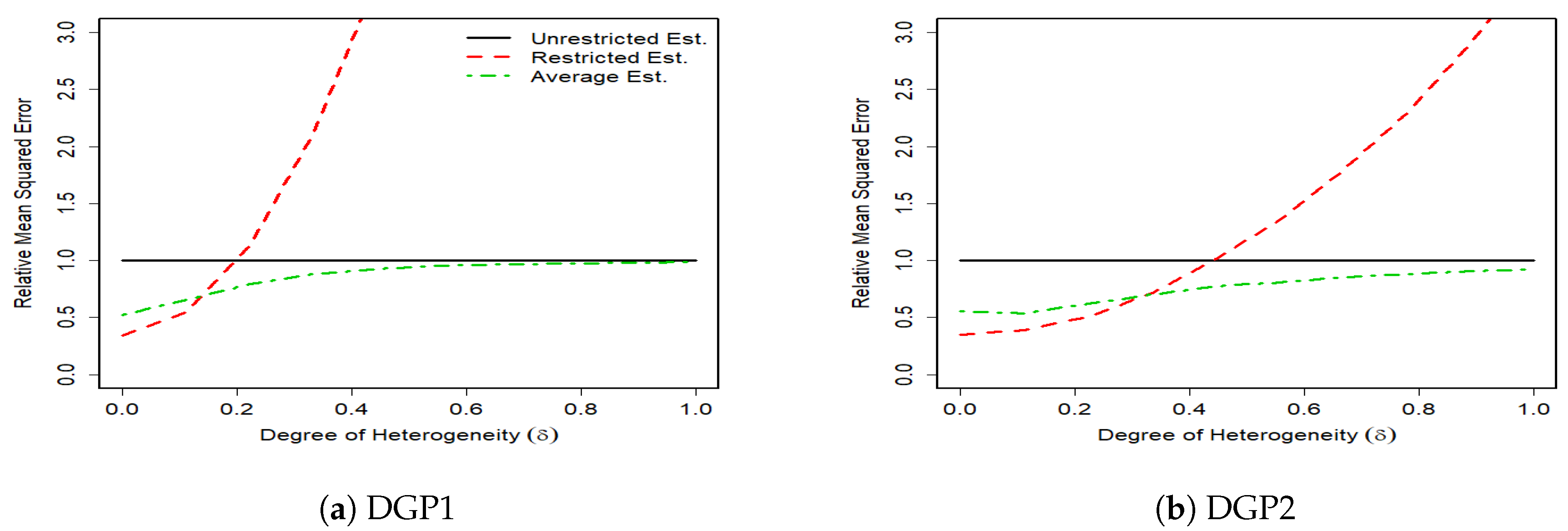
The results below are the simulation results of the model of Section 2, where and the remaining regressors are independently generated from the standard normal distribution. The sample size varies from , leading to four combinations of m, and k. is generated as while where and We consider two DGPs for generating ’s, the first one is under a complete heterogeneity in coefficients where we assume that
with and the second DGP is under a weak heterogeneity where we assume that
where denotes the largest integer value that is smaller than and takes values on a 10-point grid on .
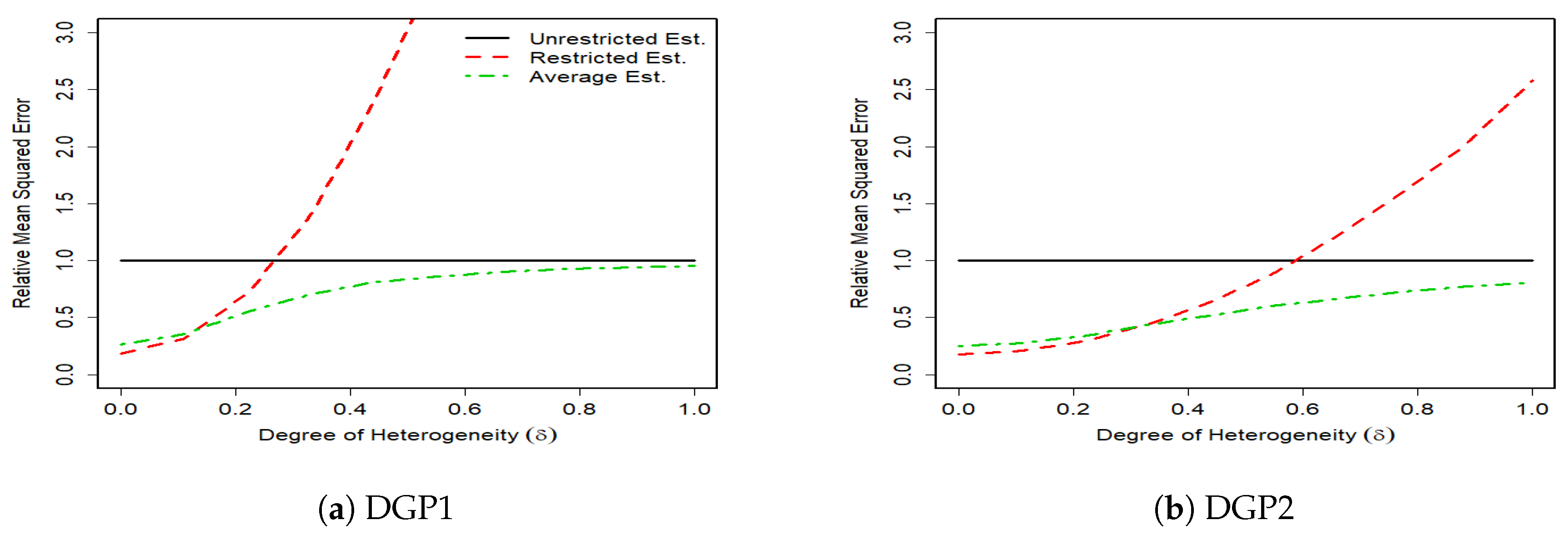
The results of 1000 monte carlo simulations are given in Figure 1, Figure 2, Figure 3 and Figure 4, where the vertical axes measure the relative mean squared error (RMSE) of the unrestricted GLS estimator, the restricted GLS estimator and the average estimator to the unrestricted GLS estimator. Hence, the RMSE of the unrestricted GLS estimator is equal to one. The horizontal axes measure the degree of parameter heterogeneity, , which is set between zero and one with grid value.
The Monte Carlo results support our theoretical findings of the previous section. The figures show that the RMSE of the average estimator for the whole parameter heterogeneity is below that of the unrestricted estimator. This shows the superiority of the average estimator relative to the unrestricted GLS estimator.
The RMSE of the average estimator in DGP1 of a complete heterogeneous SUR, is smaller than that of the restricted GLS estimator except for very small values of parameter heterogeneity (). This is expected because as takes higher values, the bias of the restricted GLS estimator increases, which then results in higher MSE. In DGP2 where the SUR is characterized by some degrees of homogeneity, the RMSE of the restricted GLS estimator remains smaller than that of the unrestricted GLS estimator for larger values of relative to DGP1. In this case, the unrestricted GLS estimator can be inferior to the restricted GLS estimator even with the presence of weak degrees of heterogeneity. This is because although the unrestricted GLS estimator is unbiased, it is inefficient, especially under small sample sizes, and a high number of regressors. In contrast, the restricted GLS estimator properly makes the use of cross equation variations and thus provides a more accurate results.
In general, we find that the average estimator performs robustly well in SUR with various degrees of heterogeneity. When there is a strong heterogeneity, the average estimator prevails. When there is a relatively weak heterogeneity, the average estimator tends to gain more from the efficiency of the restricted GLS estimator by assigning a high weight to this estimator and thus still remains one of the best choices.
6. Application: Returns to Scale in US Banking Industry
In this section we apply the average estimator studied in the previous sections to regressions of the cost system for U.S. commercial banks. We are interested in estimating the returns to scale (RTS) for these banks over the past recent years.
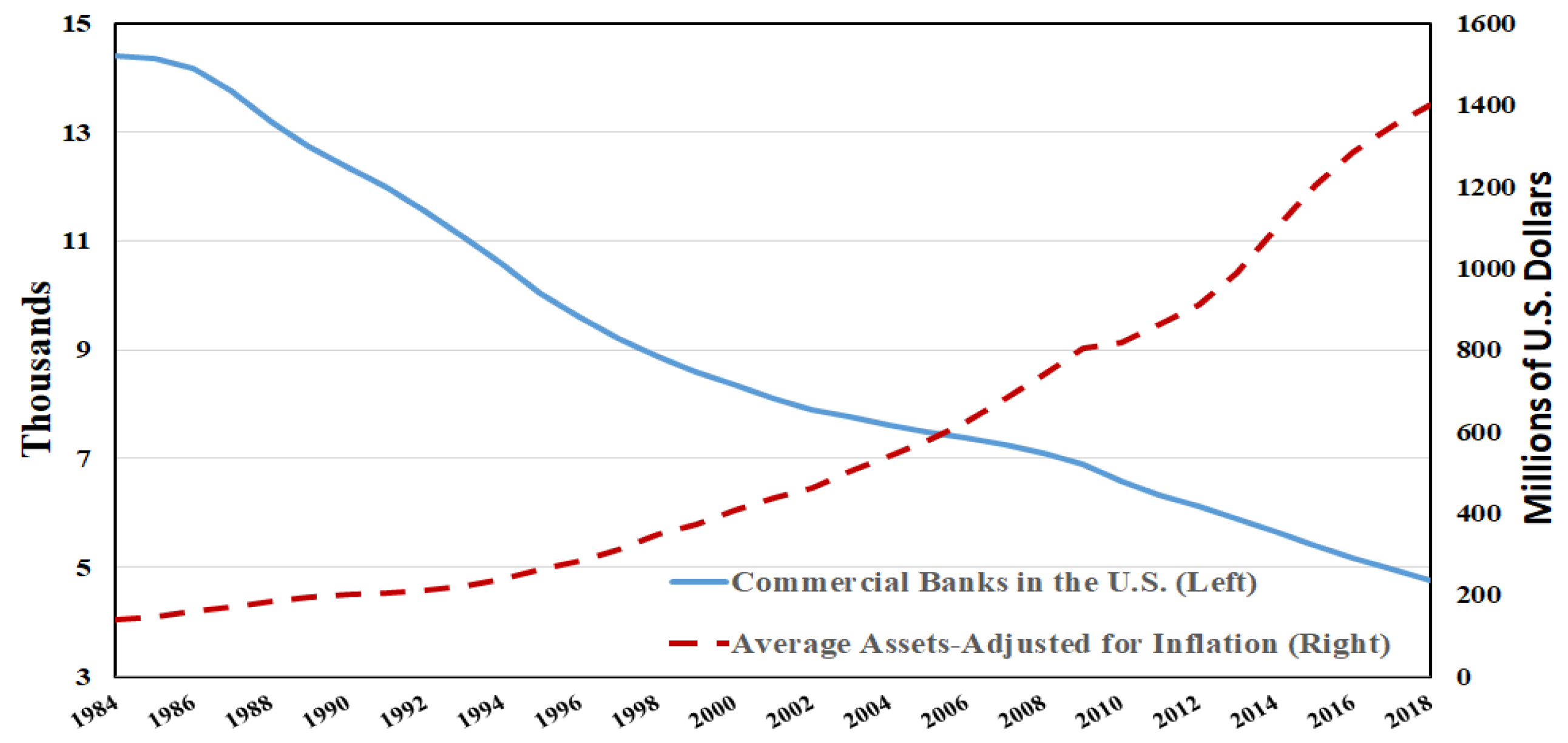
Over the past few years, the number of U.S. commercial banks fell by almost 70%, where in 1984 the total number of U.S. commercial banks was 14,391 and dropped to 4773 in 2018. Over the same period of time, the average asset value of U.S. banks (adjusted for inflation), which is also a measure of bank size, increased by about ten times, from 140 million dollars in 1984 to 1400 million dollars in 2018 (See Figure 5). To support this bank size expansion, bank executives and analysts claim that due to the changes in regulation (such as the permission of interstate branching and combination of banks) and because of technological and financial innovations (such as communication technologies, the securitization and sale of bank loans) over the past few years, the cost of production for larger banks has reduced and encouraged banks to grow larger and/or merge.
On the other hand, critics contend that this decrease in the number of operating banks, and having banks with large assets not only impact the market competition, but also result in agency problems and disproportionate benefits of government policies in favor of large banks. In particular, the financial crisis of 2007 focused attention on large financial institutions considered as “too-big-to-fail”. These together have brought attention of policy makers for regulatory limits on bank size. However, any policy intervention needs to consider the potential efficiency benefits of operating at a large scale. Therefore, estimation of scale economies and RTS is essential for analyzing the costs and benefits of any policy intervention to control the size of banks.
The estimation of scale economies and RTS for U.S. banking industry has stimulated a substantial body of studies. Older empirical studies that used data from the 1980s and 1990s did not find scale economies in banking industry except for very small banks. But recent research that used data from the 2000s, and more modern methods for estimating the banking models, has found considerably more evidence of scale economies in banking. These studies include (Hughes et al. 1996, 2000, 2001; Berger and Mester 1997; Hughes and Mester 1998, 2013; Wheelock and Wilson 2001; Feng and Serletis 2009). Most of the studies in the literature partition banks based on their asset size in groups and estimate each group independently from the other groups. However, not only there is no reason to believe these categories are set based on banks underlying technology, at the same time, it is hard to believe that these groups are not affected by some unknown factors that could have resulted in correlations between groups. Therefore, there are two issues that need to be carefully considered by researchers. First, estimating cost efficiency using all observations as one group has the advantage of smaller variance but at the same time, it means ignoring the potential heterogeneity bias due to difference in technology. Second, partitioning banks in different groups and using single-equation estimators are inefficient compared to pooled estimators which ignore heterogeneity. Hence, there is a trade-off between bias and variance efficiency between these two estimators. As the average estimator introduced in the previous sections results in the optimal balance between bias and variance efficiency, we recommend using this estimator in the estimation of the returns to scale for banking industry to obtain robust and efficient estimators.
6.1. The Model
We follow the so called “intermediation approach” framework of (Sealey and Lindley 1977), which is broadly employed in the literature. According to this approach, a bank’s balance sheet is assumed to capture the essential structure of a bank’s core business. Inputs are considered to be liabilities (core deposits and purchased funds), physical capital and labor. The inputs result in the bank’s productions which are assets (other than the physical, includes loans and trading securities).
With regard to variable specification, we define five inputs and five outputs that are the ones used in the literature. We define the following output quantities: consumer loans (), real estate loans (), loans to business and other institutions (), federal funds sold and securities purchased under agreements to resell (), and other assets (). The input variables are: labor quantities (), premises and fixed assets (), purchased funds (), interest-bearing transaction accounts (), and non-transaction accounts (). For each input , its price is obtained by dividing its total expenses by the corresponding input quantities.
For modeling the cost of banking industry, we consider a translog cost function and normalize it, so that the homogeneity (in input prices) property is automatically satisfied. We allow for individual (fixed) effects by adding intercepts in each regression, to control for specific group characteristics, heterogeneity in skills and so on. Hence, the cost equation for each group is considered as
where is the number of observations in group i (the number of banks operating within group i), and is the total cost of bank t, in group i, defined as
The cost function is symmetric which requires the imposition of the following restrictions on the parameters as below
RTS is defined as the inverse of the sum of cost elasticities. If we define the output elasticity of the model for output j of bank t in group i, as and the sum of cost elasticities as then RTS of bank t in group i is defined as Also, the RTS for group i is a vector of defined as
which is used for calculating mean, quartiles, and deciles of RTS for group i with banks, see Section 6.3.
A bank with , has increasing returns to scale, that is for one percent increase in all outputs, cost is increased by less than one percent, and the bank is operating below its efficient scale size () when .
6.2. The Data
The data we use is obtained from the Reports of Income and Condition (Call Reports)5, over the period from 2000 to 2018. We omit observations where negative values for assets, equity, outputs, and prices are reported. The summary of the data for years 2000 and 2018 is in Table 16.
Following (Feng and Serletis 2009) and others in the literature, we classify the banks into three groups which is mainly based on the standard asset size categories that are used by the Federal Financial Institutions Examination Council (FFIEC). Banks with over million in total assets are classified as Large banks, banks with assets between million and million are classified as Medium banks, and banks with under million in assets are classified as Small banks. In order to have a consistent partitions over time, the asset size caps in each year are justified upward by the growth in the CPI. Table 2 presents the number and share of banks in each group with their corresponding asset ranges for years 2000 and 2018.
6.3. Estimation
We estimate model of Equation (30) using the average estimation method developed in the previous sections for each year separately. Basically, our SUR at each year consists of three cost equations representing Large, Medium, and Small bank groups, and the observations for each regression are the operating banks data under each bank group. Since the sample size for each group is different, we face a SUR with unequal number of observations and to estimate the variance-covariance matrix (), we consider the following procedures recommended in the literature (See Schmidt 1977; Baltagi et al. 1989):
- Ignore the extra observations in estimating ;
- Use the extra observations to estimate variances. This procedure has the disadvantage of producing estimates of that are not positive definite;
- Use the extra observations to estimate variances, and modifying the estimates of covariances using the method of (Srivastava and Zaatar 1973);
- Use all observations in estimation, following the method of (Hocking and Smith 1968).
It is known in the literature that the results of the above procedures are much the same. Likewise, we find that the procedures above, generate similar results, so we only report the results of method 3.
After estimating Equation (30), we obtain the sum of cost elasticities for each bank by
where is the sum of cost elasticity of bank t in group i, and the parameters are replaced with their estimated values. Then, the RTS is calculated following Equation (33). We also obtain the RTS using the unrestricted GLS estimator, and the restricted GLS estimator.
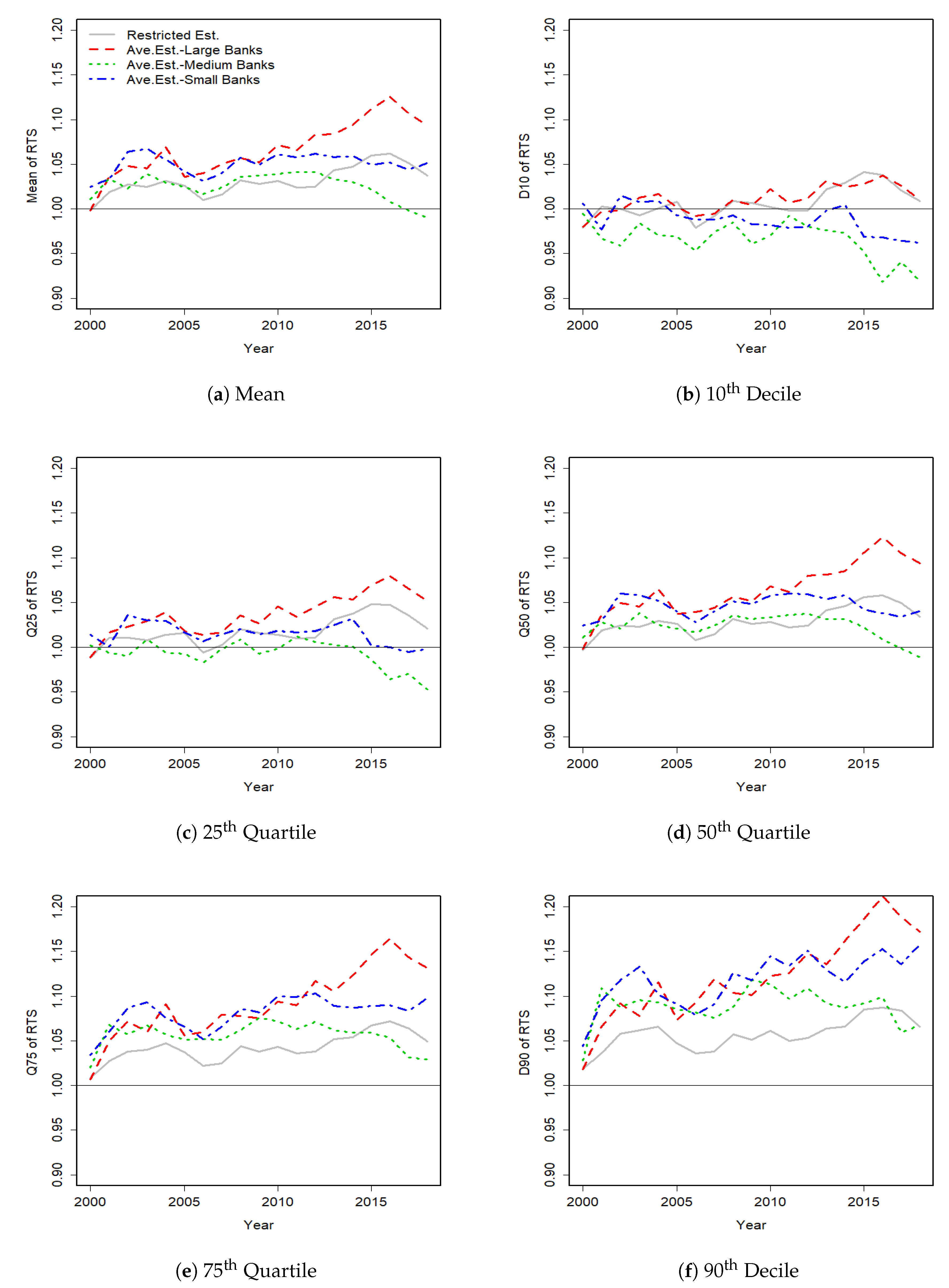
The results of years 2000, 2009 and 20187 are reported in Table 3, which presents the extreme deciles, quartiles and means of our estimated RTS using the three estimation methods. The patterns of mean, extreme deciles and quartiles for all years are plotted in Figure 6. The results base on the restricted estimator over the most recent years suggest increasing RTS at each decile. However, these results are not economically reasonable. On the other hand, we find evidence of decreasing RTS for almost 50% of Small and Medium banks using the unrestricted estimator over the most recent years. These contradicting results show the importance of the average estimator which is used to respond to this model uncertainty.
Comparing the RTS of banks using the average estimator over the sample period shows that, on average majority of banks have increasing returns to scale. In most recent years, the results exhibit more signs of cost efficiency for Large and Small banks, such that all of Large banks have increasing RTS and only less than 25% of Small banks have exhausted their cost efficiency. However, we find that more than 50% of Medium banks are operating under decreasing returns to scale near the end of the sample. The results are consistent with some recent studies (e.g., References Feng and Serletis 2009; Hughes and Mester 2013; Wheelock and Wilson 2001; Henderson et al. 2015; Mailkov et al. 2015) although we are not aware of any study from 2011 to 2018.
7. Conclusions
In this paper, we introduce an averaging estimator for a SUR model. The introduced estimator is a weighed average of an unrestricted GLS estimator which is the (Zellner 1962) estimator and a restricted GLS estimator. The weight is inversely related to a quadratic loss function which measures the weighted distance between the unrestricted and the restricted GLS estimators. The bias, MSE matrix, and risk of the average estimator using the large-sample approximations of (Nagar 1959) are derived. The superiority conditions of the average estimator in terms of the weighted mean squared error is given for any user-specific symmetric positive definite weight matrix, and is not limited to the case where the weight is the inverse of the variance-covariance matrix of the unrestricted GLS estimator.
We also provide some Monte Carlo results which support our theoretical claims. Finally, as our estimator is motivated by economic theory, we use U.S. Commercial banking data, and estimate a cost system for the banking industry to show how our estimator can be used in the applied work. We also estimate the cost system using single-equation least squares and a pooled estimator, and compare them with our proposed average estimator. We found more reliable estimation results with the cost system using our average estimator than the other estimators. We found that on average majority of banks have been operating under increasing returns to scale over the sample period from 2000 to 2018.
Author Contributions
A.M., A.U. contributed equally to the paper. All authors have read and agreed to the published version of the manuscript.
Funding
This research received no external funding.
Acknowledgments
The authors are thankful to the guest-editors and two referees for helpful and constructive comments on the subject matter of this paper.
Conflicts of Interest
The authors declare no conflict of interest.
Appendix A
Lemma A1.
Under Assumptions 1–3, we have the followings
where and , with the suffix showing the order of magnitude in probability, and
Proof.
It can be easily verified that, under Assumptions 1–3, Employing this condition, and using the standard geometric expansion for the inverse of a matrix8, for large T, we have the followings
which gives the results in Equation (A.1). Now, by using Equation (A.1), we have
also we have
By using the above results, we have
☐
Proof.
Theorem 1:
Using the results of Lemma A1, in Equation (10), we have
where and are defined below, and the suffixes show the order of magnitude in probability,
and .
Using Equation (A.5) in Equation (17), we have
where , and the last equality above holds by using the standard geometric expansion. Also, the use has been made of Equations (A.1)–(A.4). The terms with order and smaller are dropped, because they will not enter in the calculation of the bias and MSE of the average estimator up to the orders of interest.
The bias of the average estimator using the above equation up to order is
where the use has been made of
because, both and are odd functions of the error term which has a normal distribution.
The MSE matrix up to order is
where - are defined as below
Now, we obtain the expectations of - .
where the last equality holds by noting that the second term on the right-hand side of the first equality in the above equation is an odd function of normal distributions, and utilizing the following two equations below
Similarly, we have
Employing the results of Equations (A.11)–(A.16), in Equation (A.10), we obtain the MSE matrix of the average estimator up to order as below
hence the risk of the average estimator up to order can be written as
where the last inequality holds because is symmetric, therefore
see (Abadir and Magnus 2005, pp. 181–82). ☐
Proof.
Corollary 1:
Note that, using Lemma A1, we have
and
where
Therefore, it is easy to see that hence the consistency of follows. Further, by replacing by in Equation (A.10), the results in Equations (A.11), (A.13) and (A.16) remain unchange, and for Equation (A.12) we have
where the last equality holds using Equation (A.9) and noting that the terms on the right hand side of the inequality are odd functions of the error term which has a normal distribution. Also, the inequality above holds because , and are symmetric, so we have
see (Abadir and Magnus 2005, p. 344).
Therefore, the result in Equation (27) follows. ☐
References
- Abadir, Karim M., and Jan R. Magnus. 2005. Matrix Algebra. New York: Cambridge University Press. [Google Scholar]
- Baltagi, Badi H., and James M. Griffin. 1984. Short and long run effects in pooled models. International Economic Review 25: 631–45. [Google Scholar] [CrossRef]
- Baltagi, Badi H., Susan Garvin, and Stephen Kerman. 1989. Further Monte Carlo Evidence on Seemingly Unrelated Regressions with Unequal Number of Observations. Annales D’Economie et de Statistique 14: 103–15. [Google Scholar] [CrossRef]
- Baltagi, Badi H., James M. Griffin, and Weiwen Xiong. 2000. To pool or not to pool: Homogeneous versus heterogeneous estimations applied to cigarette demand. The Review of Economics and Statistics 82: 117–26. [Google Scholar] [CrossRef]
- Berger, Allen N., and Loretta J. Mester. 1997. Inside the black box: What explains differences in the efficiencies of financial institutions? Journal of Banking and Finance 21: 895–947. [Google Scholar] [CrossRef] [Green Version]
- Browning, Martin, and Jesus Carro. 2007. Heterogeneity and microeconometrics modeling. In Advances in Economics and Econometrics. Edited by Richard Blundell, Whitney Newey and Torsten Persson. Cambridge: Cambridge University Press, vol. 3, pp. 47–74. [Google Scholar]
- Choi, Hak, and Hongyi Li. 2000. Economic development and growth convergence in China. Journal of International Trade and Economic Development 9: 37–54. [Google Scholar] [CrossRef]
- Durlauf, Steven N., Andros Kourtellos, and Artur Minkin. 2001. The local Solow growth model. European Economic Review 45: 928–40. [Google Scholar] [CrossRef]
- Feng, Guohua, and Apostolos Serletis. 2009. Efficiency and productivity of the US banking industry, 1998–2005: Evidence from the Fourier cost function satisfying global regularity conditions. Journal of Applied Econometrics 24: 105–38. [Google Scholar] [CrossRef]
- Fiebig, Denzil G. 2001. Seemingly Unrelated Regression. In A Companion to Theoretical Econometrics. Edited by Badi H. Baltagi. Oxford: Blackwell, chp. 5. [Google Scholar]
- Hansen, Bruce E. 2016. Efficient Shrinkage in Parametric Models. Journal of Econometrics 190: 115–32. [Google Scholar] [CrossRef] [Green Version]
- Henderson, Daniel J., Subal C. Kumbhakar, Qi Li, and Christopher F. Parameter. 2015. Smooth coefficient estimation of a seemingly unrelated regression. Journal of Econometrics 189: 148–62. [Google Scholar] [CrossRef]
- Hocking, R. R., and Wm. B. Smith. 1968. Estimation of Parameters in the Multivariate Normal Distribution with Missing Observations. Journal of the American Statistical Association 63: 154–73. [Google Scholar]
- Hoogstrate, André J., Franz C. Palm, and Gerald A. Pfann. 2000. Pooling in dynamic panel-data models: An application to forecasting GDP growth rates. Journal of Business and Economic Studies 18: 274–83. [Google Scholar]
- Hughes, Joseph P., and Loretta J. Mester. 1998. Bank capitalization and cost: Evidence of scale economies in risk management and signaling. The Review of Economics and Statistics 80: 314–25. [Google Scholar] [CrossRef] [Green Version]
- Hughes, Joseph P., and Loretta J. Mester. 2013. Who said large banks don’t experience scale economies? Evidence from a risk-return-driven cost function. Journal of Financial Intermediation 22: 559–85. [Google Scholar] [CrossRef] [Green Version]
- Hughes, Joseph P., William Lang, Loretta J. Mester, and Choon-Geol Moon. 1996. Efficient banking under interstate branching. Journal of Money, Credit, and Banking 28: 1045–71. [Google Scholar] [CrossRef]
- Hughes, Joseph P., William Lang, Loretta J. Mester, and Choon-Geol Moon. 2000. Recovering risky technologies using the almost ideal demand system: An application to US banking. Journal of Financial Services Research 18: 5–27. [Google Scholar] [CrossRef]
- Hughes, Joseph P., Loretta J. Mester, and Choon-Geol Moon. 2001. Are scale economies in banking elusive or illusive?: Evidence obtained by incorporating capital structure and risk-taking into models of bank production. Journal of Banking and Finance 25: 2169–208. [Google Scholar] [CrossRef] [Green Version]
- James, W., and Charles Stein. 1961. Estimation with quadratic loss. Proceedings of the Fourth Berkeley Symposium on Mathematical Statistics and Probability 1: 361–80. [Google Scholar]
- Leeb, Hannes, and Benedikt M. Pötscher. 2005. Model Selection and Inference: Facts and Fiction. Econometric Theory 21: 21–59. [Google Scholar] [CrossRef] [Green Version]
- Maddala, G. S., and Wanhong Hu. 1996. The pooling problem. In The Econometrics of Panel Data. Edited by Laszlo Matyas and Patrick Sevestre. Advanced Studies in Theoretical and Applied Econometrics. Dordrecht: Springer, vol. 33, pp. 307–22. [Google Scholar]
- Maddala, G. S., Robert P. Trost, Hongyi Li, and Frederick Joutz. 1997. Estimation of short run and long run elasticities of energy demand from panel data using shrinkage estimators. Journal of Business and Economic Statistics 15: 90–100. [Google Scholar]
- Maddala, G. S., Hongyi Li, and Virendra K. Srivastava. 2001. A Comparative Study of Different Shrinkage Estimators for Panel Data Models. Annals of Economics and Finance 2: 1–30. [Google Scholar]
- Maddala, G. S. 1991. To pool or not to pool: That is the question. Journal of Quantitative Economics 7: 255–64. [Google Scholar]
- Mailkov, Emir, Diego Restrepo-Tobon, and Subal C. Kumbhakar. 2015. Estimation of banking technology under credit uncertainty. Empirical Economics 49: 185–211. [Google Scholar] [CrossRef] [Green Version]
- Nagar, Anirudh L. 1959. The Bias and Moment Matrix of the General k-Class Estimators of the Parameters in Simultaneous Equations. Econometrica 27: 575–95. [Google Scholar] [CrossRef]
- Pesaran, M. Hashem, and Ron Smith. 1995. Estimating long-run relationships from dynamic heterogeneous panels. Journal of Econometrics 68: 79–113. [Google Scholar] [CrossRef]
- Robertson, Donald, and J. Symons. 1992. Some strange properties of panel data estimators. Journal of Applied Econometrics 7: 175–89. [Google Scholar] [CrossRef] [Green Version]
- Schmidt, Peter. 1977. Estimation of Seemingly Unrelated Regressions with Unequal Numbers of Observations. Journal of Econometrics 5: 365–77. [Google Scholar] [CrossRef]
- Sclove, Stanley L. 1968. Improved estimators for coefficients in linear regression. Journal of American Statistical Association 63: 596–606. [Google Scholar]
- Sealey, Calvin W., and James T. Lindley. 1977. Inputs, outputs, and a theory of production and cost at depository financial institutions. Journal of Finance 32: 1251–66. [Google Scholar] [CrossRef]
- Srivastava, Virendra K., and Tryambkeshwar D. Dwivedi. 1979. Estimation of seemingly unrelated regression equations: A brief survey. Journal of Econometrics 10: 15–32. [Google Scholar] [CrossRef]
- Srivastava, Virendra K., and David E. A. Giles. 1987. Seemingly Unrelated Regression Models: Estimation and Inference. New York: Marcel Dekker. [Google Scholar]
- Srivastava, J. N., and M. K. Zaatar. 1973. A Monte Carlo Comparison of Four Estimators of Dispersion Matrix of a Bivariate Normal Population, Using Incomplete Data. Journal of the American Statistical Association 68: 180–83. [Google Scholar] [CrossRef]
- Srivastava, Virendra K. 1970. The efficiency of estimating seemingly unrelated regression equations. Annals of the Institute of Statistical Mathematics 22: 483–93. [Google Scholar] [CrossRef]
- Srivastava, Virendra K. 1973. The Efficiency of an Improved Method of Estimating Seemingly Unrelated Regression Equations. Journal of Econometrics 1: 341–50. [Google Scholar] [CrossRef]
- Su, Liangjun, and Qihui Chen. 2013. Testing homogeneity in panel data models with interactive fixed effects. Econometric Theory 29: 1079–135. [Google Scholar] [CrossRef] [Green Version]
- Ullah, Aman, and Huansha Wang. 2013. Parametric and Nonparametric Frequentist Model Selection and Model Averaging. Econometrics 1: 157–79. [Google Scholar] [CrossRef] [Green Version]
- Wang, Wendun, Xinyu Zhang, and Richard Paap. 2019. To Pool or Not to Pool: What is a Good Strategy? Journal of Applied Econometrics 34: 724–45. [Google Scholar] [CrossRef]
- Wheelock, David C., and Paul W. Wilson. 2001. New evidence on returns to scale and product mix among US commercial banks. Journal of Monetary Economics 47: 653–74. [Google Scholar] [CrossRef] [Green Version]
- Zellner, Arnold, and Walter Vandaele. 1975. Bayes-Stein estimators for k-means, regression and simultaneous equation models. In Studies in Bayesian Econometrics and Statistics. Edited by Stephen E. Fienberg and Arnold Zellner. Amsterdam: North-Holland Publishing Company, pp. 627–53. [Google Scholar]
- Zellner, Arnold. 1962. An Efficient Method of Estimating Seemingly Unrelated Regressions and Tests for Aggregation Bias. Journal of the American Statistical Association 57: 348–68. [Google Scholar] [CrossRef]
| 1. | Note that we do not assume that ’s are the same, nor do we assume they are different across equations. In other words, our model supports complete heterogeneity, partial heterogeneity, and complete homogeneity of regressors. |
| 2. | The second equality holds by using Equation (A.15). |
| 3. | The weight can be replaced by a positive part weight, that is, when , we assign a zero weight to the restricted estimator. It is easy to verify that the MSE of the positive part is smaller. However, it will not change the approximations, so for simplicity we do not impose it at this stage. Nevertheless, the Monte Carlo and the application results are reported using the positive part weights. |
| 4. | See Equation (A.19) in Appendix A. |
| 5. | The data from 2000–2010 is downloaded from the Federal Reserve Bank of Chicago website, and the rest of the data from 2011–2018 is downloaded from the FFIEC Central Data Repository’s Public Data Distribution website. |
| 6. | The summary of the data for other years are not reported to save the space, but it is available upon request. |
| 7. | We only report the results for these three years to save the space. However, the results for other years are available upon request. |
| 8. |
Figure 1.
RMSE of Unrestricted, Restricted and Average Estimators, for T = 100, m = 3, k = 3.
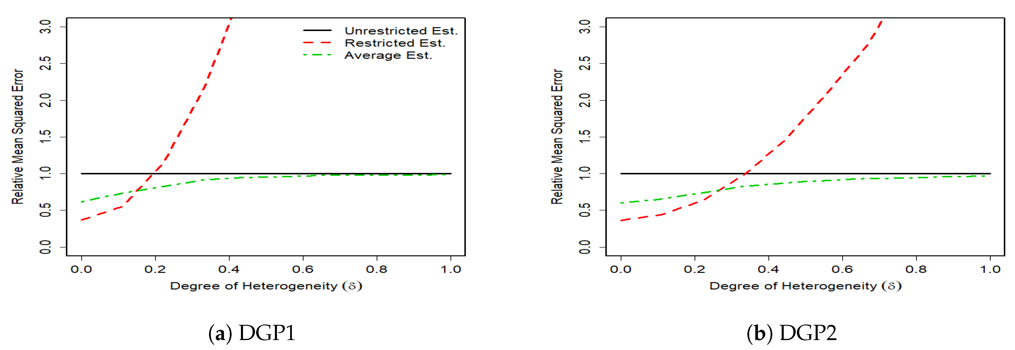
Figure 2.
RMSE of Unrestricted, Restricted and Average Estimators, for T = 100, m = 3, k = 5.

Figure 3.
RMSE of Unrestricted, Restricted and Average Estimators, for T = 100, m = 6, k = 3.
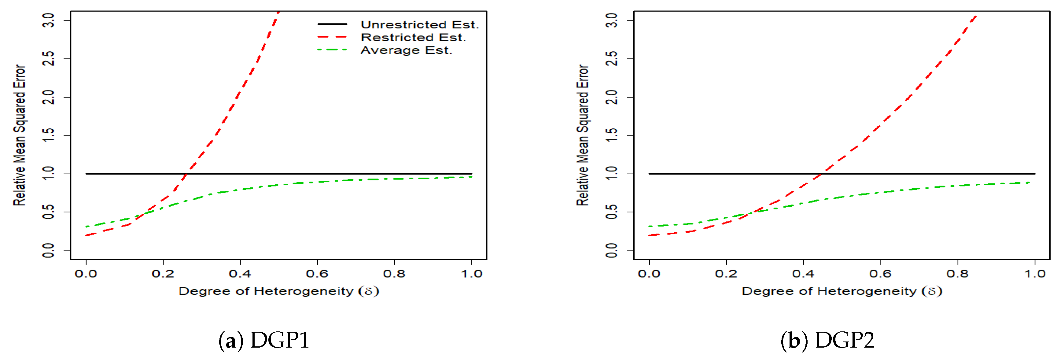
Figure 4.
RMSE of Unrestricted, Restricted and Average Estimators, for T = 100, m = 6, k = 5.

Figure 5.
United States Commercial Banks, Number and Average Assets (source: Federal Reserve Bank of St. Louis FRED database).
Figure 5.
United States Commercial Banks, Number and Average Assets (source: Federal Reserve Bank of St. Louis FRED database).

Figure 6.
RTS Estimates Using The Restricted and The Average Estimator over period 2000–2018.

Table 1.
Summary Statistics.
| Variable | Min | Max | ||
|---|---|---|---|---|
| 2000 | 2018 | 2000 | 2018 | |
| C | 136.49 | 151.78 | 18,369,359.04 | 26,757,643.39 |
| 7015.14 | 15,321.43 | 163,358.47 | 261,240.11 | |
| 6.75 | 9.61 | 12375.00 | 43,469.79 | |
| 3.20 | 0.02 | 206.53 | 48.82 | |
| 0.26 | 0.02 | 265.36 | 153.96 | |
| 0.46 | 0.06 | 49.21 | 16.82 | |
| 1.25 | 1.00 | 42,638,250.00 | 173,922,000.00 | |
| 0.25 | 170.50 | 168,465,250.00 | 686,161,250.00 | |
| 45.75 | 125.50 | 178,056,500.00 | 457,517,750.00 | |
| 89.50 | 0.25 | 144,188,250.00 | 703,099,250.00 | |
| 39.00 | 42.50 | 86,346,000.00 | 704,384,250.00 | |
| Variable | Mean | STD | ||
| 2000 | 2018 | 2000 | 2018 | |
| C | 24,454.49 | 43,803.47 | 331,091.51 | 643,872.50 |
| 26,175.32 | 49,386.16 | 7084.42 | 15,332.39 | |
| 230.31 | 265.78 | 351.89 | 920.70 | |
| 33.22 | 3.51 | 6.38 | 2.75 | |
| 14.79 | 2.43 | 9.01 | 3.87 | |
| 22.87 | 3.46 | 4.79 | 1.90 | |
| 57,014.23 | 268,717.11 | 754,295.15 | 4,722,816.78 | |
| 175,843.57 | 881,915.93 | 2,961,928.59 | 15,632,429.24 | |
| 206,836.22 | 929,043.01 | 2,423,963.16 | 10,526,805.47 | |
| 192,820.92 | 862,701.61 | 2,985,314.66 | 16,392,980.08 | |
| 85,019.93 | 842,793.39 | 1,554,035.20 | 16,868,329.90 | |
Note: All variables except – are measured in thousands of dollars.
Table 2.
Banks Asset Size Classes.
| Bank Groups | Asset Size (in Millions of Dollars of the Year) | Number of Banks | Share of Banks |
|---|---|---|---|
| 2000 | |||
| Large Banks | Assets ≥ 500 | 739 | 8.9 |
| Medium Banks | 100 ≤ Assets < 500 | 2946 | 35.5 |
| Small Banks | Assets < 100 | 4620 | 55.6 |
| 2018 | |||
| Large Banks | Assets ≥ 729 | 988 | 19.8 |
| Medium Banks | 146≤ Assets <729 | 2298 | 46.1 |
| Small Banks | Assets < 146 | 1704 | 34.1 |
Table 3.
Summary of estimates of returns to scale.
| Bank Size | Estimator | Estimates of RTS | |||||
|---|---|---|---|---|---|---|---|
| Mean | |||||||
| 2000 | |||||||
| Restricted | 0.979 | 0.988 | 0.997 | 1.008 | 1.019 | 0.998 | |
| Large Banks | Unrestricted | 0.971 | 0.985 | 0.998 | 1.009 | 1.021 | 0.996 |
| Average Estimator | 0.980 | 0.989 | 0.998 | 1.007 | 1.018 | 0.998 | |
| Medium Banks | Unrestricted | 0.969 | 0.992 | 1.017 | 1.043 | 1.071 | 1.019 |
| Average Estimator | 0.995 | 1.002 | 1.011 | 1.020 | 1.028 | 1.011 | |
| Small Banks | Unrestricted | 0.997 | 1.014 | 1.034 | 1.055 | 1.075 | 1.035 |
| Average Estimator | 1.006 | 1.014 | 1.024 | 1.034 | 1.044 | 1.025 | |
| 2009 | |||||||
| Restricted | 1.007 | 1.016 | 1.026 | 1.038 | 1.051 | 1.028 | |
| Large Banks | Unrestricted | 1.001 | 1.025 | 1.053 | 1.080 | 1.108 | 1.055 |
| Average Estimator | 1.004 | 1.026 | 1.051 | 1.075 | 1.101 | 1.052 | |
| Medium Banks | Unrestricted | 0.956 | 0.990 | 1.032 | 1.079 | 1.125 | 1.038 |
| Average Estimator | 0.961 | 0.993 | 1.031 | 1.076 | 1.118 | 1.037 | |
| Small Banks | Unrestricted | 0.979 | 1.013 | 1.049 | 1.085 | 1.124 | 1.050 |
| Average Estimator | 0.983 | 1.015 | 1.048 | 1.082 | 1.118 | 1.049 | |
| 2018 | |||||||
| Restricted | 1.009 | 1.021 | 1.034 | 1.049 | 1.066 | 1.037 | |
| Large Banks | Unrestricted | 1.009 | 1.052 | 1.100 | 1.140 | 1.184 | 1.098 |
| Average Estimator | 1.010 | 1.052 | 1.094 | 1.132 | 1.172 | 1.093 | |
| Medium Banks | Unrestricted | 0.915 | 0.950 | 0.988 | 1.030 | 1.070 | 0.989 |
| Average Estimator | 0.919 | 0.953 | 0.989 | 1.029 | 1.068 | 0.990 | |
| Small Banks | Unrestricted | 0.960 | 0.997 | 1.042 | 1.104 | 1.166 | 1.054 |
| Average Estimator | 0.962 | 0.998 | 1.040 | 1.098 | 1.158 | 1.051 | |
Note: Decile, quartile and mean estimates of RTS for the restricted, unrestricted, and average estimators. , , , , and are the lower decile, the upper decile, the lower quartile, median and upper quartile, respectively.
© 2020 by the authors. Licensee MDPI, Basel, Switzerland. This article is an open access article distributed under the terms and conditions of the Creative Commons Attribution (CC BY) license (http://creativecommons.org/licenses/by/4.0/).
Share and Cite
MDPI and ACS Style
Mehrabani, A.; Ullah, A. Improved Average Estimation in Seemingly Unrelated Regressions. Econometrics 2020, 8, 15. https://0-doi-org.brum.beds.ac.uk/10.3390/econometrics8020015
AMA Style
Mehrabani A, Ullah A. Improved Average Estimation in Seemingly Unrelated Regressions. Econometrics. 2020; 8(2):15. https://0-doi-org.brum.beds.ac.uk/10.3390/econometrics8020015
Chicago/Turabian StyleMehrabani, Ali, and Aman Ullah. 2020. "Improved Average Estimation in Seemingly Unrelated Regressions" Econometrics 8, no. 2: 15. https://0-doi-org.brum.beds.ac.uk/10.3390/econometrics8020015
Note that from the first issue of 2016, this journal uses article numbers instead of page numbers. See further details here.