Bayesian Model Averaging Using Power-Expected-Posterior Priors


1
Statistics Lab, Department of Mathematics, National Technical University of Athens, Zografou Campus, 15780 Athens, Greece
2
Computational and Bayesian Statistics Lab, Department of Statistics, Athens University of Economics and Business, 10434 Athens, Greece
*
Author to whom correspondence should be addressed.
Econometrics 2020, 8(2), 17; https://0-doi-org.brum.beds.ac.uk/10.3390/econometrics8020017
Submission received: 18 February 2020
/
Revised: 15 March 2020
/
Accepted: 6 May 2020
/
Published: 11 May 2020
(This article belongs to the Special Issue Bayesian and Frequentist Model Averaging)
Abstract
:This paper focuses on the Bayesian model average (BMA) using the power–expected– posterior prior in objective Bayesian variable selection under normal linear models. We derive a BMA point estimate of a predicted value, and present computation and evaluation strategies of the prediction accuracy. We compare the performance of our method with that of similar approaches in a simulated and a real data example from economics.
1. Introduction
We consider the variable–selection problem for normal regression models. Let us denote the model space by , consisting of all combinations of available covariates. Then, for every model , the likelihood is specified by
where is a multivariate random variable expressing the response for each subject, is a design/data matrix containing the values of the explanatory variables in its columns, is the identity matrix, is a vector of length with the effects of each covariate on the response data , and is the error variance of the model.
Under the Bayesian model choice perspective, we need to introduce priors on the model space and on the parameters of each competing model. With respect to the prior distribution on the parameters in each model, because we are not confident about any given set of regressors as explanatory variables, little prior information on their regression coefficients can be expected. This argument alone justifies the need for an objective model choice approach in which vague prior information is assumed. Hence, within each model, we consider default prior distributions on the regression coefficients and error variance. Default priors for normal regression parameters are improper and thus cannot be used, since they lead to an indeterminate Bayes factor (Berger and Pericchi 2001). This has urged the objective Bayesian community to develop various methodologies to overcome the problem of prior specification in model–selection problems. One of the proposed approaches is the expected–posterior prior (EPP) of Pérez and Berger (2002). Starting from a baseline (typically improper) prior of parameters of model , the approach relies on the utilization of the device of “imaginary training samples". If we denote by the imaginary training sample of size , the EPP is defined as
where is the posterior distribution of for model using the baseline prior and data . A usual choice of is , i.e., the marginal likelihood, evaluated at , for a reference model under the baseline prior . Then, for , it is straightforward to show that . Under the variable–selection problem, the usual choice is to consider to be the “null" model with only the intercept; this is the choice considered in this paper in the last two experimental sections. In a more general setting, we can assume that the response variable is known to be explained by variables (including the intercept) that form the reference model , and, by some subset of p, other explanatory variables that form models under comparison. Thus, in the rest of the paper, we assume that is nested to all other models under comparison. Under this more general case, we denote by the parameters of , and by , its design matrix (assumed to be of full rank). Since is nested in every other competing model , with parameters and design matrix (again assumed to be of full rank), we can henceforth assume that and , so that is a “common” parameter between the two models, and is a model–specific. The use of a “common” parameter in nested model comparison is often made to justify the employment of the same, potentially improper, prior on across models. This usage is becoming standard–see, for example, Bayarri et al. (2012); Consonni et al. (2018). It can be justified if, without essential loss of generality, we assume that the model has been parametrized in an orthogonal fashion, so that . When is the “null" model, the above assumption can be easily justified, if we assume that, again without loss of generality, the columns of design matrix X of the full model, containing all p available explanatory variables, have been centred on their corresponding means, this makes the covariates orthogonal to the intercept, and gives the intercept an interpretation that is “common” to all models.
When comparing models and , under the EPP methodology, imaginary design matrices , with rows, should also be introduced; . In what follows, we denote by and those imaginary design matrices under models and respectively. As before, we assume that those matrices are of full rank. Furthermore we denote by . The selection of minimal training sample size was proposed by Berger and Pericchi (2004) to make information content of the prior as small as possible, and this is an appealing idea. Then, can be extracted from original design matrix by randomly selecting from the n rows.
To diminish the effect of training samples, Fouskakis et al. (2015) generalized the EPP approach by introducing the power–expected–posterior (PEP) priors, combining ideas from the power–prior approach of Ibrahim and Chen (2000) and the unit–information–prior approach of Kass and Wasserman (1995). As a first step, the likelihoods involved in the EPP formula are raised to the power and are then density–normalized. This power parameter could be then set equal to the size of training sample to represent information equal to one data point. Fouskakis et al. (2015) further set ; this choice gives rise to significant advantages, for example, when covariates are available, it results in automatic choice ; therefore, the selection of a training sample and its effects on the posterior model comparison are avoided while still holding prior information content at one data point. In the last two sections of this paper, this recommended setup () was used.
Specifically, the PEP prior under model is defined as
with
As before, we choose
where
Regarding the baseline prior, under model , we use
while under model we use
where and are the unknown normalizing constants of and respectively. Usual choices for and are (resulting to the reference prior) or and (resulting in the dependence Jeffreys prior). In the last two experimental sections of this paper, the former case was used. Under the above setup, the PEP prior of the reference model is equal to the corresponding baseline prior, that is, .
One of the advantages of using PEP priors (or EPPs for ) is that the impropriety of baseline priors causes no indeterminacy of the Bayes factor. More specifically, the resulting Bayes factor for comparing model to takes the form of
where, for ,
Therefore, returning back to Equation (3), we have that
As is obvious from Equation (4), normalizing constants and are cancelled out; thus, there are no issues of indeterminacy of the Bayes factor.
Under the above setup, Fouskakis and Ntzoufras (2020) proved that PEP priors (or EPPs for ) for comparing model to are given by
with
where . In the above expression,
is proper and ; i.e., the reference prior for the baseline model .
Using Equation (5), if , following the results of Fouskakis and Ntzoufras (2020), the PEP prior under model can be represented as normal scale mixture distribution:
where denotes the density of d-dimensional normal distribution with mean and covariance matrix , evaluated at , and denotes the prior distribution of parameter g under model . The hyper–prior for g is given by
with and .
The above form of the PEP prior offers great advantages; given g, posterior distributions and marginal likelihoods can be easily derived in closed-form expressions. However, even without conditioning on g, those distributions can be written in terms of Appell hypergeometric functions, and therefore again be derived. Detailed formulas that are also used in the next two sections can be found in Fouskakis and Ntzoufras (2020). In the following, a parameter of importance is also the shrinkage w that, under the PEP prior, is equal to ; its posterior mean, used in the following sections, was analytically derived in Fouskakis and Ntzoufras (2020).
Bayesian model averaging (BMA) is a standard Bayesian approach that combines predictions or estimates of a quantity of interest over different models that are weighted according to their posterior model probabilities. BMA efficiently incorporates model uncertainty that naturally exists in all statistical problems. By handling model uncertainty via BMA, we obtain posterior distributions and posterior credible intervals that are more realistic, and we avoid single model inference that can be severely biased or overconfident in terms of uncertainty. Moreover, several authors empirically showed BMA results lead to better predictive procedures (see for example Fernandez et al. 2001a; Ley and Steel 2009, 2012; Raftery et al. 1997). For more details on BMA, also see Hoeting et al. (1999), Steel (2016, 2019) for BMA implementation in economics.
In this work, we derive Bayesian model averaging estimates under the PEP prior. Furthermore, we present different computational solutions for deriving the Bayes factor and performing the Bayesian model average, which are applied in a simulated and a real-life dataset.
2. BMA Point Prediction Estimates
Let us consider a set of models , with design matrices , where the covariates of the design matrix (of the reference model ) are included in all models. Thus. we assume as before that and . We are interested in quantifying uncertainty about the inclusion or exclusion of additional columns/covariates of model . Under this setup, for any model , given a set of new values of explanatory variables , we are interested in estimating the corresponding posterior predictive distribution . Following Liang et al. (2008), for each model , we consider the BMA prediction–point estimator, which is the optimal under squared error loss and is given by
where is the given set of new values of all explanatory variables. Detailed derivations of posterior means and are provided in Section 4.1 of Fouskakis and Ntzoufras (2020). If we now further assume that , then the posterior means of the coefficients are considerably simplified to
where and . Hence, assuming in a similar fashion that , the posterior predictive mean, under model , is now reduced to
and the corresponding BMA point prediction estimate is now given by
The expected value of the posterior distribution of in Equation (9) is given by
while posterior model probabilities in Equation (9) can be calculated using the closed–form expression of the marginal likelihood
where is the hypergeometric function of two variables or Appell hypergeometric function, , and , with and being the coefficients of determination of models and , respectively. For the detailed derivation of Equations (10) and (11), see Fouskakis and Ntzoufras (2020, Sections 4.2 and 5.2, respectively).
3. Computation and Evaluation of BMA Prediction
For small–to–moderate sample spaces, it is straightforward to implement full enumeration of the model space and calculate the marginal likelihoods by using Equation (11) and the Appell hypergeometric function. This function is available, for example, in the R package tolerance; see Function F1. Alternatively, it can be calculated using standard methods for the computation of one–dimensional integrals.
In our applications of Section 4 and Section 5, we did not observe any “precision” problems with the calculation of the Appell hypergeometric function. Nevertheless, in the case of overflow issues in the implementation of this approach (e.g., for large n), using a simple Laplace approximation (preferably on ) can be an effective and relatively precise alternative.
Another way to estimate each marginal likelihood is by using simple Monte Carlo schemes. For example, we can simply generate values of g from its posterior distribution (see Fouskakis and Ntzoufras 2020), or some good approximations of the posterior distribution of g, and then calculate the final marginal likelihood as the mean of the conditional marginal likelihoods, which can be easily derived in closed-form expressions over all sampled values of g.
In the case of large model space, when full enumeration is not computationally feasible, we can implement a Markov chain Monte Carlo (MCMC) algorithm that could be considered as a simple extension of (Madigan and York 1995) with two steps, since all needed quantities are analytically available given g. In the first step, we update the model indicator by using a simple Metropolis step where acceptance probability is a simple function of the posterior model odds; in the second step, we generate g from the marginal posterior distribution of g.
Using any of the above computational approaches, and assuming that is the “null” model, we can obtain a BMA prediction estimate by using Equation (9) and implementing the following procedure:
- For every model :
- Implement Equation (9) to calculate , as the weighted average of over all models using posterior model probabilities as weights.
Evaluation of prediction accuracy or goodness of fit can be achieved by the square root of the mean of the squares (RMSE) between the observed and the fitted/predicted values or the corresponding mean absolute deviation (MAD) given by
respectively. In the illustrated example of Section 4, we present the RMSE and the MAD for the maximum–a–posteriori (MAP) model and the median–probability (MP) model, as well as for the full BMA (with all models), the BMA for the 10 highest a–posteriori models, and for the models with posterior odds versus the MAP model of at least .
In addition, in Section 5, we compare the predictive performance of PEP with that of other mixtures of g-priors. For the application considered in Section 5, we randomly partition the sample B times in modelling and validation subsamples of a fixed size. Then, we calculate the BMA–log predictive score (BMA–LPS); see, for example, Fernandez et al. (2001b). Specifically, for each partition, we denote by the modelling subsample of size , and by the validation subsample of size , where . The BMA–LPS then is given by
where
with and denoting the posterior (given the data in the modelling subsample) and prior probabilities of model , respectively. Smaller values of BMA-LPS indicate better performance.
Concerning the computation of Equation (12), it is obvious that, when full enumeration is feasible, we can calculate the BMA–LPS by using Equation (13) for all models under consideration; for the evaluation of marginal likelihoods in the numerator and denominator, we use Equation (11). In the case where the number of predictors (and thus the number of induced models) does not allow full enumeration, there are three direct computational approaches that we may use:
- Model search using algorithm (Madigan and York 1995): this approach can be used since the marginal likelihood is readily available, but it is not very efficient, especially for large model spaces, since both the numerator and the denominator in Equation (13) are greatly affected by the number of visited models, and hence by the number of iterations of the algorithm.
- g–conditional algorithm: hyper–parameter g is generated by its marginal posterior distribution; then, we use the conditional on g marginal likelihood to move through the model space; this is the approach used by Ley and Steel (2012). Under this setup, is estimated bywhere T is the total number of MCMC iterations, is the generated value of g at iteration t, and is the visited model at iteration t.
- Fully Bayesian variable–selection MCMC: density is estimated by the MCMC average of the sampling–density function of each visited model , evaluated at , for each generated set of the model parameters. This is the approach we used in Section 5. More specifically, we implemented the Gibbs variable–selection approach of Dellaportas et al. (2002).
4. Simulation Study
In this section, we illustrate the proposed methodology in simulated data. We compare the performance of the PEP prior and the intrinsic prior, the latest as presented in Fouskakis and Ntzoufras (2020) and in Womack et al. (2014), by calculating the RMSE and the MAD under different BMA setups, as explained in Section 3.
We considered 100 datasets of observations with covariates. We ran two different scenarios. Under Scenario 1 (independence), all covariates were generated from multivariate normal distribution with mean vector and covariance matrix , while the response is generated from
for . Under Scenario 2 (collinearity), the response was again generated from Equation (14), but this time, only the first 10 covariates were generated from multivariate normal distribution with mean vector and covariance matrix , while
for .
With covariates, there are only 32,768 models to compare; we were able to conduct full enumeration of the model space, obviating the need for a model–search algorithm in this example.
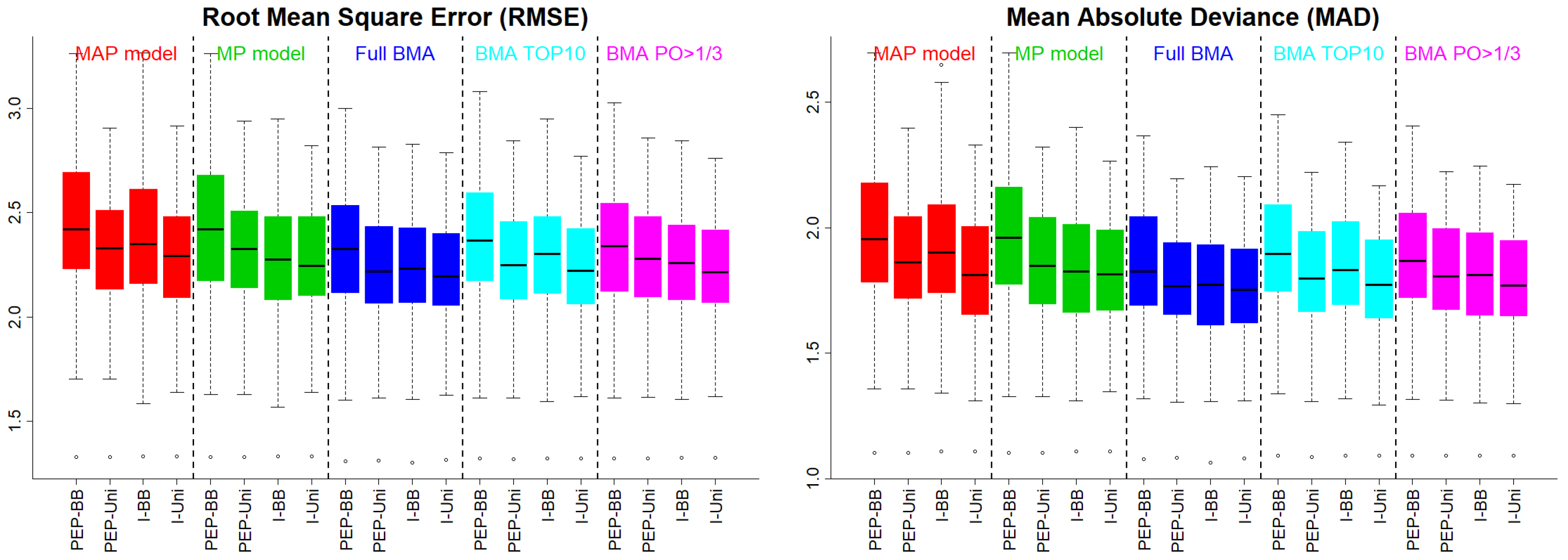
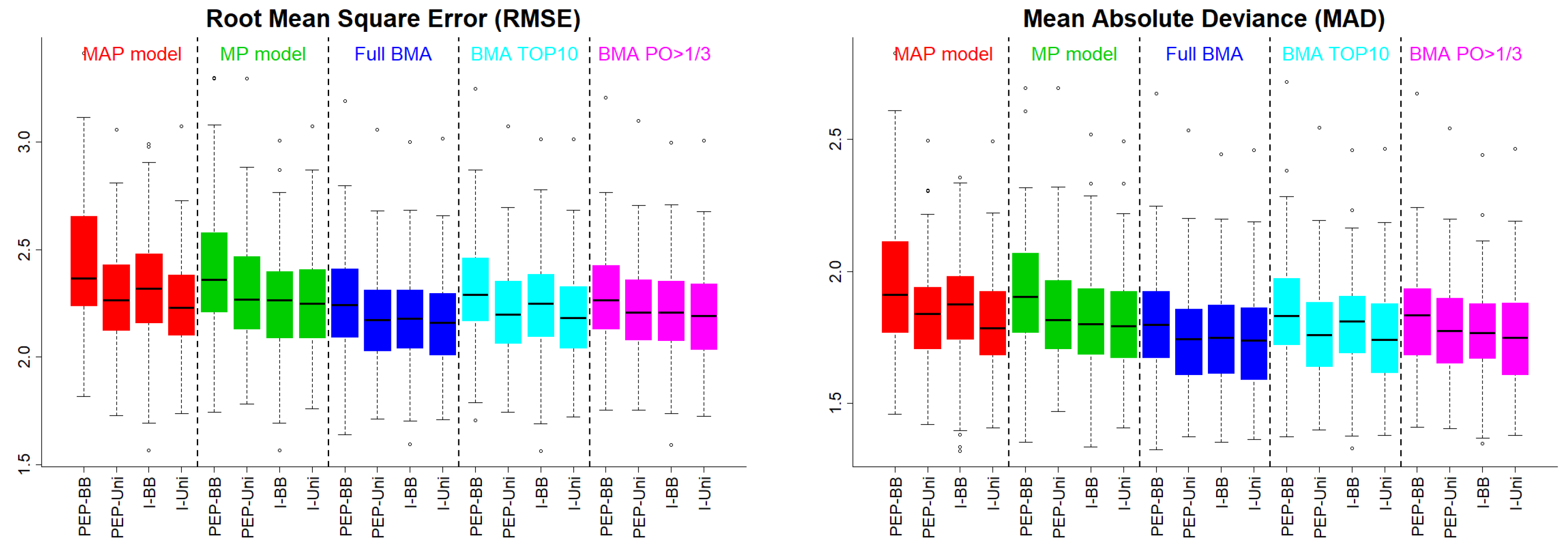
Regarding the prior on the model space, we considered the uniform prior on the model space (uni), as well as the uniform prior on model size (BB), as a special case of the beta–binomial prior (Scott and Berger 2010); thus, in what follows, we compare the following methods: PEP–BB, PEP–Uni, I–BB and I–Uni; the first two names denote the PEP prior under the uniform prior on the model space and the uniform prior on model size, respectively; the last two names denote the intrinsic prior under the uniform prior on the model space and the uniform prior on model size, respectively.
Figure 1 presents the RMSE and the MAD under Scenario 1. The uniform prior on the model space (PEP–Uni and I–Uni) supported MAP models with better predictive abilities. Similar was the picture when we implemented BMA with any of the three approaches. PEP–BB behaved slightly worse than the rest of the methods, suggesting that the BB prior is possibly undesirable for PEP, since it over–shrank effects to zero.
In Figure 2, we present the RMSE and the MAD under Scenario 2. The pattern was the same as that under the independence case scenario.
5. FLS Dataset: Cross-Country Growth GDP Study
In this section, we consider the dataset of Fernandez et al. (2001b) (also known as the FLS dataset) that contains potential regressors for modelling average per capita growth over the period of 1960–1992 for a sample of countries. More details on the dataset can be found in Fernandez et al. (2001b).
Emphasis was given to the posterior mean model size, to the posterior distributions of g and w, and to the comparison of the predictive performance of PEP with that of other mixtures of g–priors using the BMA–LPS as presented in Section 3. To calculate the BMA–LPS, we randomly partitioned the sample times in modelling and validation subsamples of fixed sizes and , respectively, as in Ley and Steel (2012).
Regarding the prior on the model space, we considered the uniform prior on model space (uni), the uniform prior on model size (BB), and the beta–binomial prior with elicitation (BBE) using the recommended value of , as in Ley and Steel (2009); Ley and Steel (2012).
Results under the PEP prior were compared to the ones obtained under (a) the hyper– prior, with the recommended value of , as in Liang et al. (2008); and (b) the benchmark prior, with the recommended value of , as in Ley and Steel (2012). Further comparisons with other mixtures of g–priors could be made using the results of Section 8.1 in Ley and Steel (2012). Thus, in what follows, we make 9 comparisons in total; we use labels PEP–uni, PEP–BB, PEP–BBE, Hyper––uni, Hyper––BB, Hyper––BBE, Benchmark–uni, Benchmark–BB, and Benchmark–BBE to denote the PEP, the hyper–, and the benchmark priors (under the recommended values of their hyper–parameters), respectively, combined with the different priors on the model space, i.e., the uniform on model space, the uniform on model size, and the beta–binomial with elicitation (), respectively.
A fully Bayesian variable selection MCMC algorithm was used, as described in Section 3; we used MCMC chains of 10,000 length after a burn-in of 1,000, which was found to be sufficient for the convergence of the quantities of interest here.
In Figure 3 we present box plots of BMA–LPS values over the 50 validation subsamples. Hyper– and benchmark priors seemed to perform slightly better, but in general, we could infer that no noticeable differences were observed regarding the predictive performance of each combination of priors on the model parameters and model space.
In Figure 4, we present box plots of the posterior mean model size of visited models over the 50 modelling subsamples. When all three priors (PEP, hyper– and benchmark) were combined with the beta–binomial prior (with and without elicitation) on model space we end up visiting models, with considerably lower, on average, size. The pattern is the same under all three priors used for the model parameters; the size, on average, of the visiting models is higher under the uniform prior on model space, followed by the beta–binomial without elicitation and the beta–binomial with elicitation. Regarding the sampling variability of the posterior mean model size, this is higher (for all three priors used on model parameters) when the beta–binomial without elicitation is used, followed by the beta–binomial with elicitation and the uniform prior on model space. The hyper– and benchmark priors produced results that almost coincide when combined with the same prior on the model space. On the other hand, the PEP prior, seems to result in an approach that is more parsimonious, in contrast to the approaches resulting under the hyper– and the benchmark priors when comparisons are made under the same prior on model space; the differences are sharper when the beta–binomial (with and without elicitation) prior on model space is used.
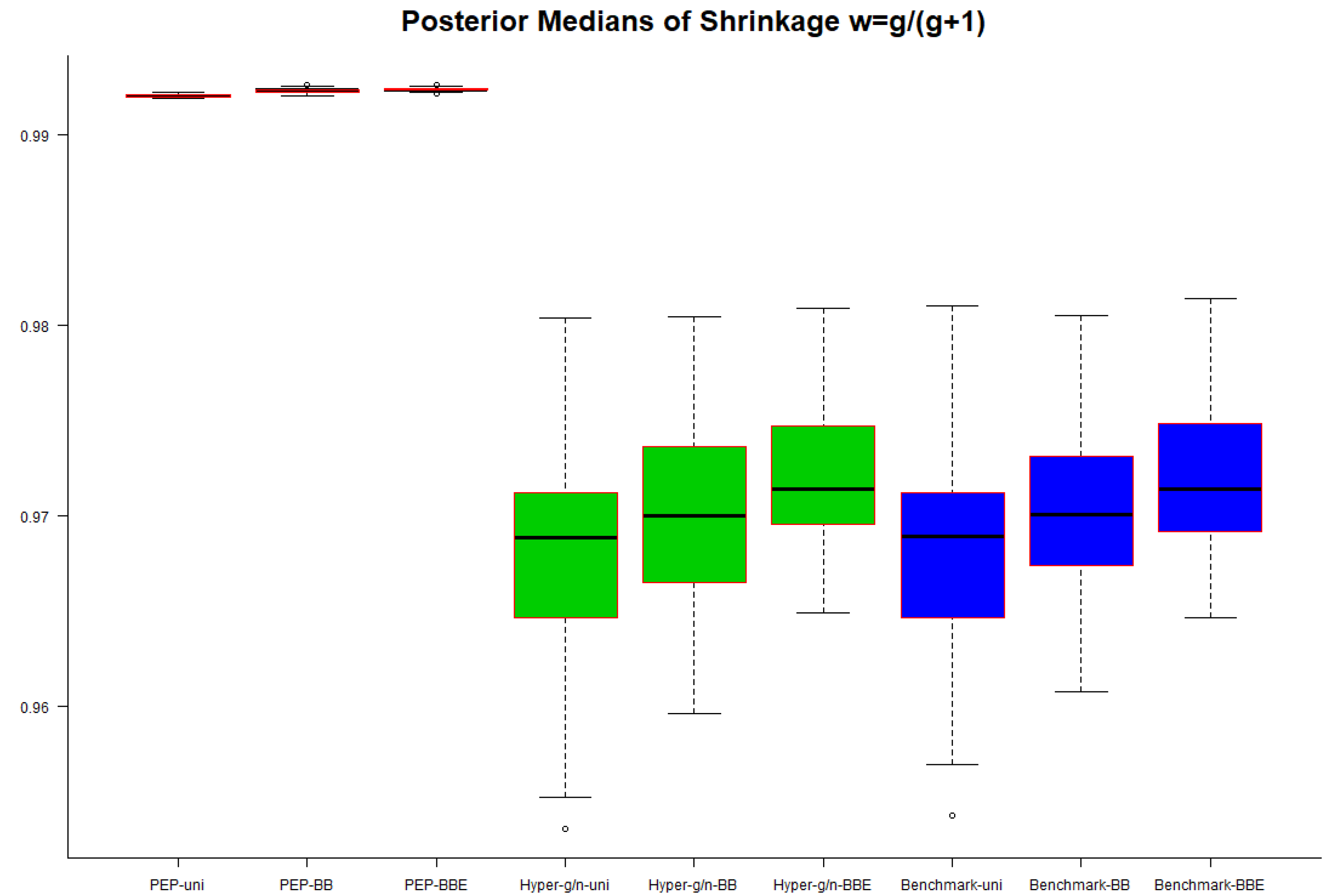
Box plots of the posterior medians of g (on a log scale) over the 50 modelling subsamples are provided in Figure 5. For all three priors used on model parameters, posterior medians of g are slightly smaller under the uniform prior on model space, followed by the beta–binomial prior without elicitation and the beta–binomial prior with elicitation. Additionally, posterior medians of g are smallest for the hyper– and benchmark priors and largest under the PEP prior using any of the three priors on model space. Furthermore, we observe that the sampling variability of posterior medians across the 50 subsamples under the PEP prior was very small.
This behavior was expected, since the PEP prior induced a lower bound on g that was equal to n. In addition, in Figure 6, we present box plots of the posterior medians of the shrinkage factor w over the 50 modelling subsamples. Findings, as expected, were similar as the ones from Figure 5; a–posteriori, the median of the global shrinkage factor w under the PEP prior was close to the value of 1, implying that the induced method was more parsimonious across models, and the prior was generally noninformative (and less informative compared to the hyper– and benchmark priors) within each model, since most of the information was taken from the data.
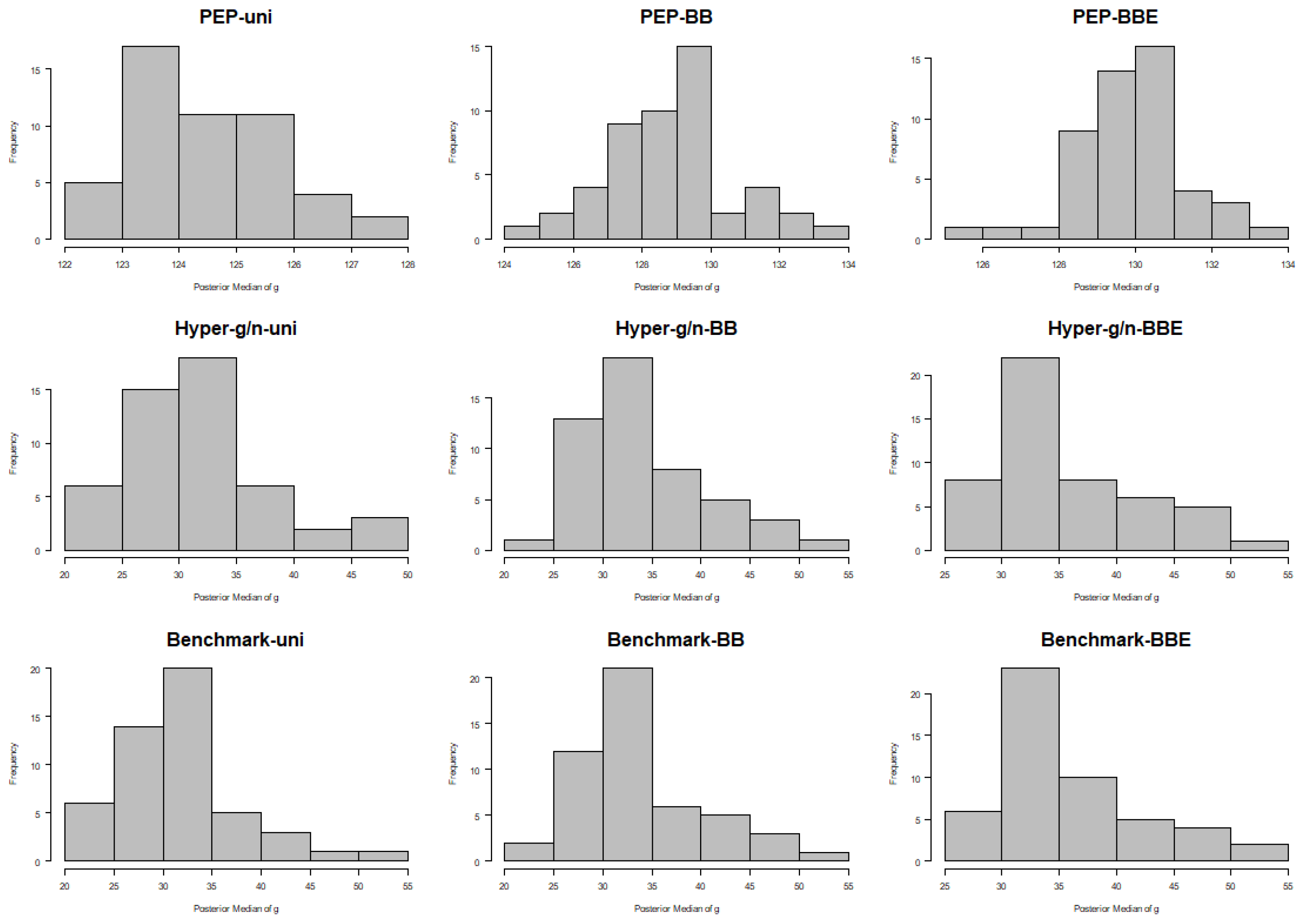
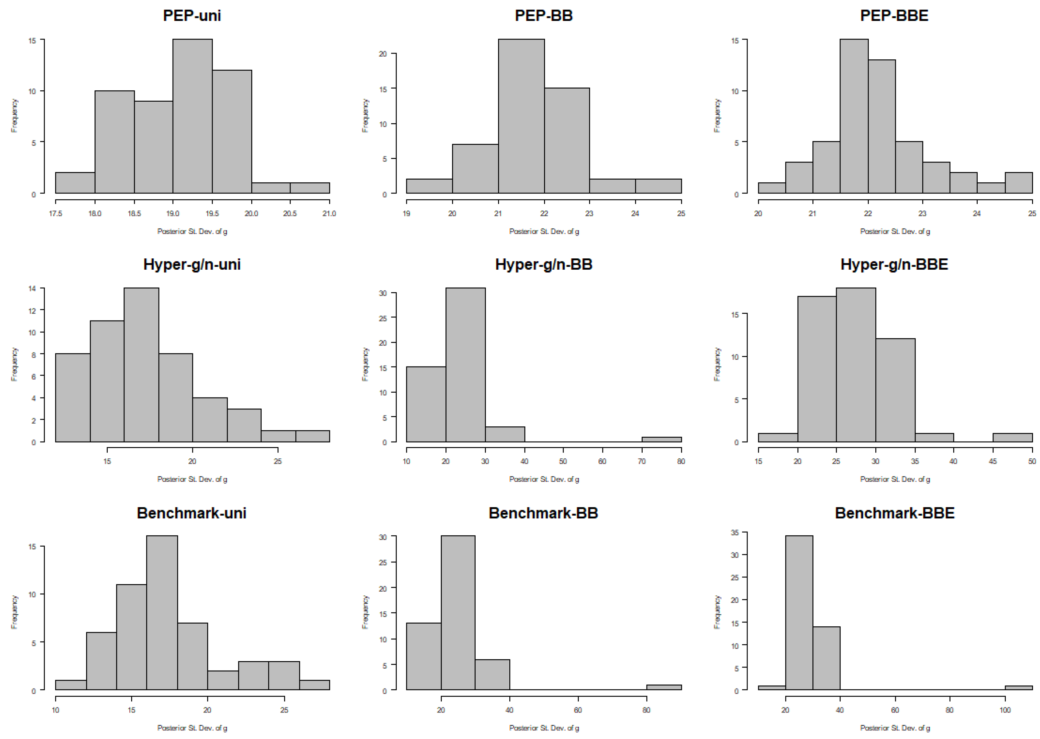
Following the comment of a referee stating that the posterior values of g under the PEP prior are concentrated at the lower bound (which is equal to n), thus implying that the PEP prior degenerates to a fixed prior choice of g, we further present the histograms of the posterior medians and the posterior standard deviations of g for the FLS data; see Figure 7 and Figure 8, respectively. From these histograms, it is obvious that the posterior medians were not concentrated at the left bound.
The range of posterior medians of g (across the 50 modelling subsamples of size ) was actually from 122 to 128 for PEP–Uni and slightly higher for PEP–BB and PEP–BBE; see Figure 7. Moreover, posterior standard deviations were in the range of 17.5–21 for PEP–Uni and slightly higher for PEP–BB and PEP–BBE; see Figure 8. Clearly, PEP priors were not concentrated at the lower bound (which was equal to ), and standard deviations were large enough to allow for posterior uncertainty on g. On the other hand, both hyper– and benchmark priors supported posterior medians of g in the range of 20–55 that, in some subsamples, was much lower than that of the sample size of . This raised the question of whether all model parameters are over–shrunk toward the prior mean for specific subsamples. Moreover, posterior standard deviations under both hyper– and benchmark priors for g fell in the range of 10–30 under the Uni and BB priors on model space, and even higher under the BB prior (10–80 and 10–90 for hyper– and benchmark priors respectively) and under the BBE prior (15–50 and 10–110 for hyper– and benchmark priors respectively). We raise two points for discussion here. First, the variability of the posterior distribution of g across the 50 modelling subsamples was high, although all datasets were subsamples from the same larger dataset. Second, for some modelling subsamples, standard deviation was very high (compared to the subsample size) that, in combination with the low posterior medians, may result in a “waste” of valuable posterior probability in informative prior choices (within each model), and to the inflation of the posterior probability of irrelevant models with low practical usefulness.
6. Discussion
In this article, we derived a Bayesian model average (BMA) estimate of a predicted value on a variable–selection problem in normal linear models using the power–expected–posterior (PEP) prior. Furthermore, we presented computation and evaluation strategies of the prediction accuracy, and compared the performance of our method with that of similar approaches in a simulated and a real data example from economics.
An interesting point of discussion is the fact that the lower bound imposed on g seemed to drive the final results under the PEP prior. Of course, we could still specify the PEP prior with smaller values of in order to consider different weighting of the imaginary data. By this way, the bound (via the choice of ) could be lower; thus, we might leave g to take values in a wider range. Nevertheless, under the recommended PEP prior specification, detailed analysis with the FLS data did demonstrate that the posterior medians of g across the 50 modelling subsamples were far away from the lower bound. Furthermore, posterior standard deviations were high enough to allow for satisfactorily posterior uncertainty for g. On the other hand, using other hyper–priors for g, like the hyper–g or the hyper–, which do not restrict the range of values for g, resulted in high posterior standard deviations of g that, in combination with low posterior medians, may result in a “waste” of valuable posterior probability in informative prior choices (within each model), and to the inflation of the posterior probability of irrelevant models with low practical usefulness. This behavior has two side effects: (a) the posterior probability of the MAP model was considerably lower than the one obtained by methods with fixed prior choices for g, and (b) the posterior inclusion probabilities for the nonimportant covariates would be inflated towards 0.5; see Dellaportas et al. (2012) for an empirical illustration within the hyper–g prior setup.
Our results implied that the PEP prior was more parsimonious than its competitors. We do not claim that this property is always the best practice in variable–selection problems. The choice of parsimony or sparsity depends on the problem at hand. When we have a sparse dataset where important covariates are very few, then the PEP prior probably acts in a better way than other competitors that may spend a large portion of the posterior probability to models that are impractical in terms of dimension and sparsity.
Author Contributions
The two authors have equally contributed in the development of the ideas, the theoretical developments, the implementation of the proposed methodology, the data related illustrations and the writing of the article.
Funding
The two authors were indirectly funded by their institutions (National Technical University of Athens and Athens University of Economics). No further funding was available for this research.
Acknowledgments
We wish to thank the academic editor and the two reviewers for the comments that greatly strengthened the paper. All authors have read and agreed to the published version of the manuscript.
Conflicts of Interest
The authors declare no conflict of interest.
References
- Bayarri, Maria J., James O. Berger, Anabel Forte, and Gonzalo García-Donato. 2012. Criteria for Bayesian model choice with application to variable selection. Annals of Statistics 40: 1550–77. [Google Scholar] [CrossRef] [Green Version]
- Berger, James O., and Luis R. Pericchi. 2001. Objective Bayesian methods for model selection: Introduction and comparison. In Model Selection. Institute of Mathematical Statistics Lecture Notes. Monograph Series 38; Beachwood: IMS, pp. 135–207. [Google Scholar]
- Berger, James O., and Luis R. Pericchi. 2004. Training samples in objective model selection. Annals of Statistics 32: 841–69. [Google Scholar] [CrossRef] [Green Version]
- Consonni, Guido, Dimitris Fouskakis, Brunero Liseo, and Ioannis Ntzoufras. 2018. Prior distributions for objective Bayesian analysis. Bayesian Analysis 13: 627–79. [Google Scholar] [CrossRef]
- Dellaportas, Petros, Jonathan J. Forster, and Ioannis Ntzoufras. 2002. On Bayesian model and variable selection using MCMC. Statistics and Computing 12: 27–36. [Google Scholar] [CrossRef]
- Dellaportas, Petros, Jonathan J. Forster, and Ioannis Ntzoufras. 2012. Joint specification of model space and parameter space prior distributions. Statistical Science 27: 232–46. [Google Scholar] [CrossRef]
- Fernandez, Carmen, Eduardo Ley, and Mark F. J. Steel. 2001a. Benchmark priors for Bayesian model averaging. Journal of Econometrics 100: 381–427. [Google Scholar] [CrossRef] [Green Version]
- Fernandez, Carmen, Eduardo Ley, and Mark F. J. Steel. 2001b. Model uncertainty in cross-country growth regressions. Journal of Applied Econometrics 16: 563–576. [Google Scholar] [CrossRef]
- Fouskakis, Dimitris, and Ioannis Ntzoufras. 2020. Power-Expected-Posterior priors as mixtures of g-priors. arXiv arXiv:2002.05782. [Google Scholar]
- Fouskakis, Dimitris, Ioannis Ntzoufras, and David Draper. 2015. Power-expected-posterior priors for variable selection in Gaussian linear models. Bayesian Analysis 10: 75–107. [Google Scholar] [CrossRef] [Green Version]
- Hoeting, Jennifer A., David Madigan, Adrian E. Raftery, and Chris T. Volinsky. 1999. Bayesian Model Averaging: A Tutorial. Statistical Science 14: 382–417. [Google Scholar]
- Ibrahim, Joseph G., and Ming-Hui Chen. 2000. Power prior distributions for regression models. Statistical Science 15: 46–60. [Google Scholar]
- Kass, Robert E., and Larry Wasserman. 1995. A reference Bayesian test for nested hypotheses and its relationship to the Schwarz criterion. Journal of the American Statistical Association 90: 928–34. [Google Scholar] [CrossRef]
- Ley, Eduardo, and Mark F. J. Steel. 2009. On the effect of prior assumptions in Bayesian model averaging with applications to growth regression. Journal of Applied Econometrics 24: 651–74. [Google Scholar] [CrossRef] [Green Version]
- Ley, Eduardo, and Mark F. J. Steel. 2012. Mixtures of g-priors for Bayesian model averaging with economic applications. Journal of Econometrics 171: 251–66. [Google Scholar] [CrossRef] [Green Version]
- Liang, Feng, Rui Paulo, German Molina, Merlise A. Clyde, and Jim O. Berger. 2008. Mixtures of g priors for Bayesian variable selection. Journal of the American Statistical Association 103: 410–23. [Google Scholar] [CrossRef]
- Madigan, David, and Jeremy York. 1995. Bayesian graphical models for discrete data. International Statistical Review 63: 215–32. [Google Scholar] [CrossRef] [Green Version]
- Pérez, José M., and James O. Berger. 2002. Expected-posterior prior distributions for model selection. Biometrika 89: 491–511. [Google Scholar] [CrossRef]
- Raftery, Adrian E., David Madigan, and Jennifer A. Hoeting. 1997. Bayesian model averaging for linear regression models. Journal of the American Statistical Association 92: 179–91. [Google Scholar] [CrossRef]
- Scott, James G., and James O. Berger. 2010. Bayes and empirical-Bayes multiplicity adjustment in the variable-selection problem. The Annals of Statistics 38: 2587–619. [Google Scholar] [CrossRef] [Green Version]
- Steel, Mark F. J. 2016. Bayesian model averaging. In Wiley StatsRef: Statistics Reference Online. Edited by Balakrishnan Narayanaswamy, Theodore Colton, Brian Everitt, Walter Piegorsch, Fabrizio Ruggeri and Jef Teugels. New Jersey: John Wiley & Sons, Ltd., pp. 1–7. [Google Scholar]
- Steel, Mark F. J. 2019. Model Averaging and its Use in Economics. arXiv arXiv:1709.08221. [Google Scholar]
- Womack, Andrew J., Luis León-Novelo, and George Casella. 2014. Inference from intrinsic Bayes’ procedures under model selection and uncertainty. Journal of the American Statistical Association 109: 1040–53. [Google Scholar] [CrossRef]
Figure 1.
Simulation scenario 1. Predictive measures for maximum–a–posteriori (MAP) and median–probability (MP) models and Bayesian model averaging (BMA) using all models (full) and highest a–posteriori models [best 10 models and models with posterior odds (PO) versus the MAP model of at least ].
Figure 1.
Simulation scenario 1. Predictive measures for maximum–a–posteriori (MAP) and median–probability (MP) models and Bayesian model averaging (BMA) using all models (full) and highest a–posteriori models [best 10 models and models with posterior odds (PO) versus the MAP model of at least ].

Figure 2.
Simulation scenario 2. Predictive measures for maximum–a–posteriori (MAP) and median–probability (MP) models and Bayesian model averaging (BMA) using all models (full) and highest a–posteriori models [best 10 models and models with posterior odds (PO) versus the MAP model of at least ].
Figure 2.
Simulation scenario 2. Predictive measures for maximum–a–posteriori (MAP) and median–probability (MP) models and Bayesian model averaging (BMA) using all models (full) and highest a–posteriori models [best 10 models and models with posterior odds (PO) versus the MAP model of at least ].

Figure 3.
FLS dataset: box plots of BMA log predictive scores over 50 prediction subsamples.
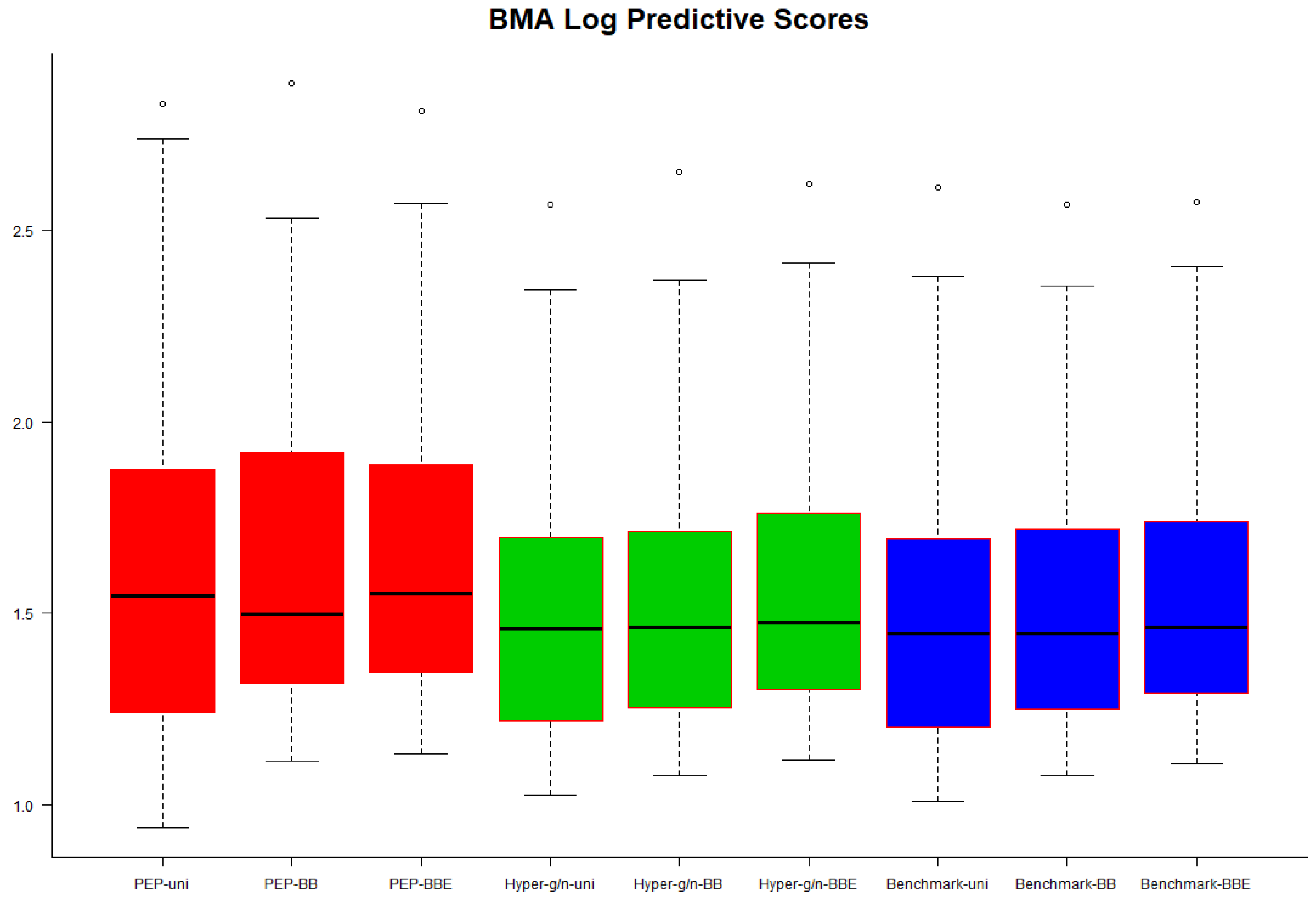
Figure 4.
FLS dataset: box plots of posterior mean model size of visited models over 50 prediction subsamples.
Figure 4.
FLS dataset: box plots of posterior mean model size of visited models over 50 prediction subsamples.
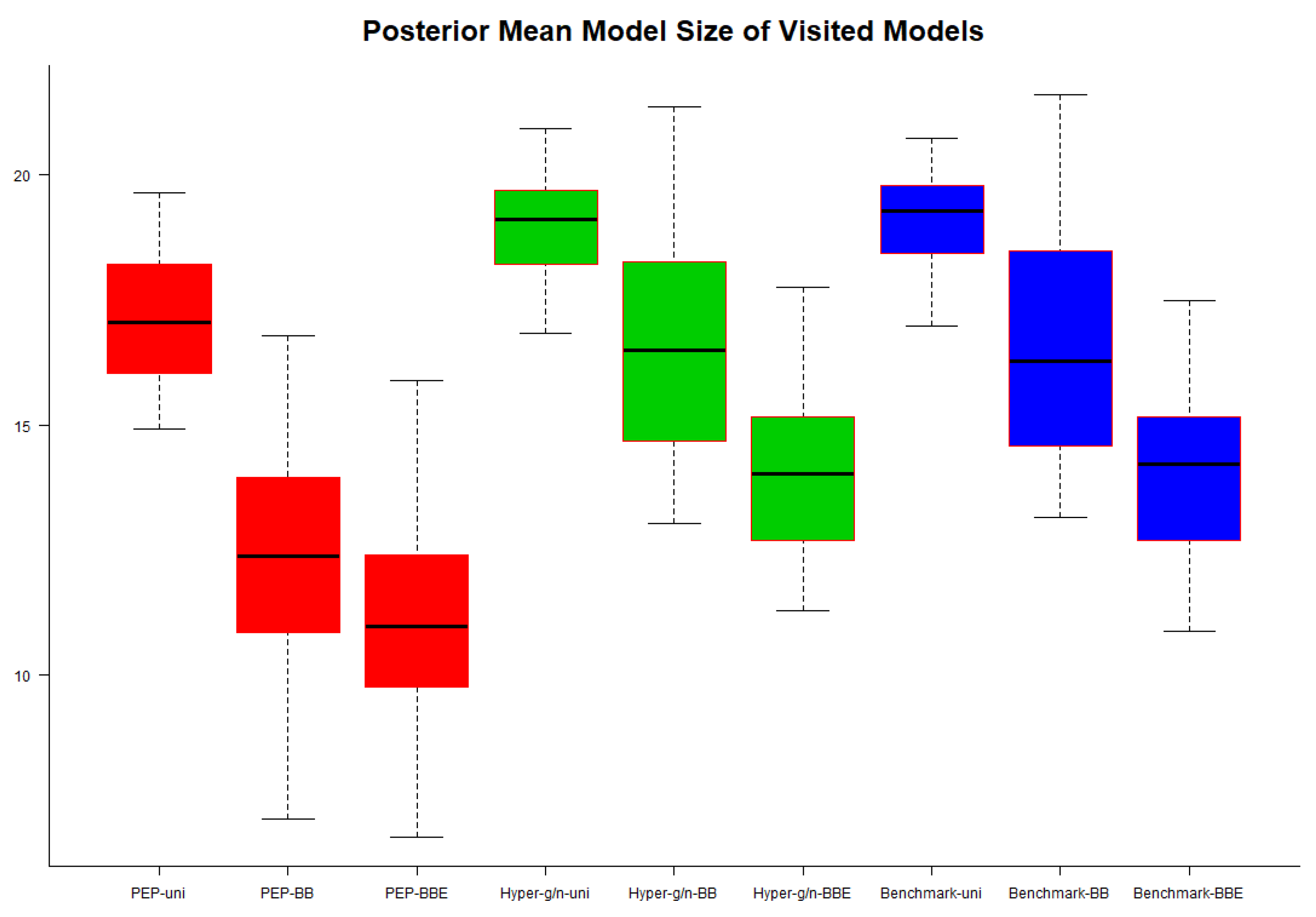
Figure 5.
FLS dataset: box plots of log posterior medians of g over 50 prediction subsamples.
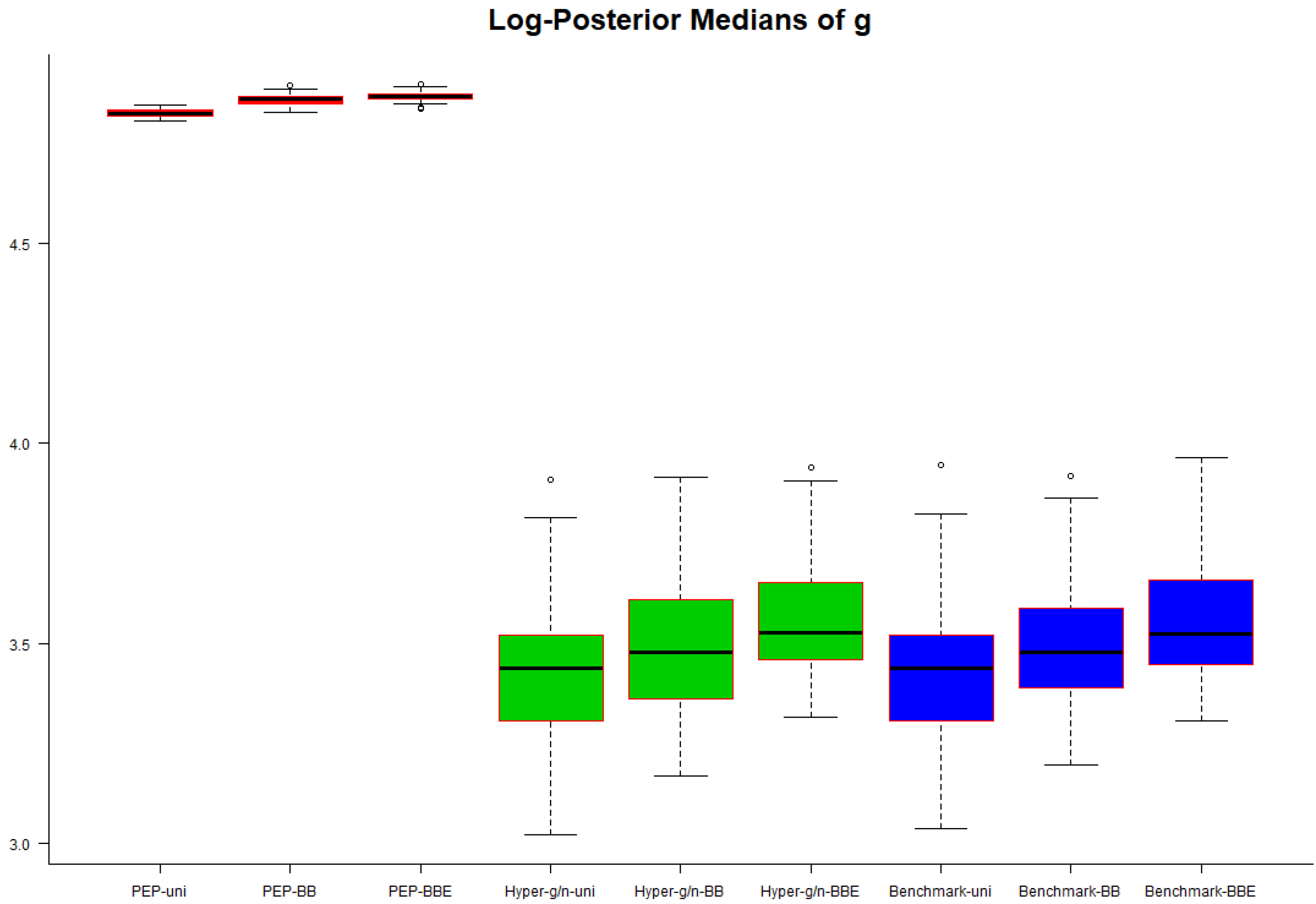
Figure 6.
FLS dataset: box plots of posterior medians of the shrinkage factor w over 50 prediction subsamples.
Figure 6.
FLS dataset: box plots of posterior medians of the shrinkage factor w over 50 prediction subsamples.

Figure 7.
Histograms of posterior medians of g for all methods under comparison for the FLS data.

Figure 8.
Histograms of posterior standard deviations of g for all methods under comparison for the FLS data.
Figure 8.
Histograms of posterior standard deviations of g for all methods under comparison for the FLS data.

© 2020 by the authors. Licensee MDPI, Basel, Switzerland. This article is an open access article distributed under the terms and conditions of the Creative Commons Attribution (CC BY) license (http://creativecommons.org/licenses/by/4.0/).
Share and Cite
MDPI and ACS Style
Fouskakis, D.; Ntzoufras, I. Bayesian Model Averaging Using Power-Expected-Posterior Priors. Econometrics 2020, 8, 17. https://0-doi-org.brum.beds.ac.uk/10.3390/econometrics8020017
AMA Style
Fouskakis D, Ntzoufras I. Bayesian Model Averaging Using Power-Expected-Posterior Priors. Econometrics. 2020; 8(2):17. https://0-doi-org.brum.beds.ac.uk/10.3390/econometrics8020017
Chicago/Turabian StyleFouskakis, Dimitris, and Ioannis Ntzoufras. 2020. "Bayesian Model Averaging Using Power-Expected-Posterior Priors" Econometrics 8, no. 2: 17. https://0-doi-org.brum.beds.ac.uk/10.3390/econometrics8020017
Note that from the first issue of 2016, this journal uses article numbers instead of page numbers. See further details here.