Article

Triple the Gamma—A Unifying Shrinkage Prior for Variance and Variable Selection in Sparse State Space and TVP Models

by
Annalisa Cadonna
,
Sylvia Frühwirth-Schnatter
* and
Peter Knaus
Department of Finance, Accounting and Statistics, WU Vienna University of Economics and Business, 1020 Vienna, Austria
*
Author to whom correspondence should be addressed.
Submission received: 9 December 2019 / Revised: 6 April 2020 / Accepted: 29 April 2020 / Published: 20 May 2020
(This article belongs to the Special Issue Bayesian and Frequentist Model Averaging)

Abstract

:
Time-varying parameter (TVP) models are very flexible in capturing gradual changes in the effect of explanatory variables on the outcome variable. However, in particular when the number of explanatory variables is large, there is a known risk of overfitting and poor predictive performance, since the effect of some explanatory variables is constant over time. We propose a new prior for variance shrinkage in TVP models, called triple gamma. The triple gamma prior encompasses a number of priors that have been suggested previously, such as the Bayesian Lasso, the double gamma prior and the Horseshoe prior. We present the desirable properties of such a prior and its relationship to Bayesian Model Averaging for variance selection. The features of the triple gamma prior are then illustrated in the context of time varying parameter vector autoregressive models, both for simulated dataset and for a series of macroeconomics variables in the Euro Area.

1. Introduction

Model selection in a high-dimensional setting is a common challenge in statistical and econometric inference. The introduction of Bayesian model averaging (BMA) techniques in the statistical literature (Brown et al. 2002; Cottet et al. 2008; Raftery et al. 1997) has led to many interesting applications, see, among others, (Frühwirth-Schnatter and Tüchler 2008; Kleijn and van Dijk 2006; Koop and Potter 2004; Sala-i-Martin et al. 2004) for early references in econometrics.
Selecting explanatory variables for possibly very high-dimensional regression problems though shrinkage priors is an attractive alternative to BMA which relies on discrete mixture priors, see Bhadra et al. (2019) for an excellent review. There is a vast and growing literature on shrinkage priors for regression problems that focuses on the following aspects. First, how to choose sensible priors for high-dimensional model selection problems in a Bayesian framework, second, how to design efficient algorithms to cope with the associated computational challenges and third, to investigate, both from a theoretical and a practical viewpoint, how such priors perform in high-dimensional problems.
A striking duality exists in this very active area between Bayesian and traditional approaches. For many shrinkage priors, the mode of the posterior distribution obtained in a Bayesian analysis can be regarded as a point estimate from a regularization approach, see Fahrmeir et al. (2010) and Polson and Scott (2012a). One such example is the popular Lasso (Tibshirani 1996) which is equivalent to a double-exponential shrinkage prior in a Bayesian context (Park and Casella 2008). However, the two approaches differ when it comes to selecting penalty parameters that impact the sparsity of the solution. One advantage of the Bayesian framework in this context is that the penalty parameters are considered to be unknown hyperparameters which can be learned from the data. Such “global-local” shrinkage priors (Polson and Scott 2011) adjust to the overall degree of sparsity that is required in a specific application through a global shrinkage parameter and separate signal from noise through local, individual shrinkage parameters.
While the inclusion of potentially many explanatory variables though shrinkage priors in regression models is addressed in a vast literature, the use of shrinkage priors for more general econometric models in time series analysis, such as state space models and time-varying parameter (TVP) models is, in comparison, less well-studied. Sparsity in the context of such models refers to the presence of a few large variances among many (nearly) zero variances in the latent state processes that drive the observed time series data. A common goal in this setting is to recover a few dynamic states, driven by such a state space model, among many (nearly) constant coefficients. As shown by Frühwirth-Schnatter and Wagner (2010), this variance selection problem can be cast into a variable selection problem in the non-centered parametrization of a state space model. Once this link has been established, shrinkage priors that are known to perform well in high-dimensional regression problems can be applied to variance selection in state space models, as demonstrated for the Lasso (Belmonte et al. 2014) and the normal-gamma (Bitto and Frühwirth-Schnatter 2019; Griffin and Brown 2017).
Despite this already existing variety, we introduce a new shrinkage prior for variance selection in sparse state space and TVP models in the present paper called triple gamma prior, as it has a representation involving three gamma distributions. This prior can be related to various shrinkage priors that were found to be useful for high-dimensional regression problems, such as the generalized beta mixture prior (Armagan et al. 2011), and contains the popular Horseshoe prior (Carvalho et al. 2009, 2010) as a special case. Furthermore, the half-t and the half Cauchy (Gelman 2006; Polson and Scott 2012b), suggested as robust alternatives to the inverse gamma distribution for variance parameters in hierarchical models, as well as the Lasso and the double gamma, are special cases of the triple gamma. In this context, the triple gamma can also be regarded as an extension of the scaled beta2 distribution (Pérez et al. 2017).
Among Bayesian shrinkage priors, usually a clear distinction is made between two-group mixture or spike-and-slab priors and continuous shrinkage priors, of which the triple gamma is a special case. An important contribution of the present paper is to show that the triple gamma provides a bridge between these two approaches and has the following property which is favourable both in sparse and dense situations. One of the hyperparameters allows high concentration over the region in the shrinkage profile that is relevant for shrinking noise, while the other hyperparameter allows high concentration over the region that prevents overshrinking of signals. This allows the triple gamma prior to exhibit behavior that very much resembles Bayesian model averaging based on discrete spike-and-slab priors, with a strong prior concentration at the corner solutions where some of the variances are nearly zero. While this is reminiscent of the Horseshoe prior, the shrinkage profile induced by the triple gamma is more flexible than that of a Horseshoe. Thanks to the estimation of the hyperparemters, it is not constrained to be symmetric around one half, enabling adaption to varying degrees of sparsity in the data.
The triple gamma prior also scores well from a computational perspective. While exploring the full posterior distribution for spike-and-slab priors leads to computational challenges due to the combinatorial complexity of the model space, Bayesian inference based on Markov chain Monte Carlo (MCMC) methods is straightforward for continuous shrinkage priors, exploiting their Gaussian-scale mixture representation (Bitto and Frühwirth-Schnatter 2019; Makalic and Schmidt 2016). An extension of these schemes to the triple gamma prior is fairly straightforward.
We will study the empirical performance of the triple gamma for a challenging setting in econometric time series analysis, namely for time-varying parameter vector autoregressive models with stochastic volatility (TVP-VAR-SV models). Since the influential paper of Primiceri (2005) (see Del Negro and Primiceri (2015) for a corrigendum), this model has become a benchmark for analyzing relationships between macroeconomic variables that evolve over time, see Nakajima (2011), Koop and Korobilis (2013), Eisenstat et al. (2014), Chan and Eisenstat (2016), Feldkircher et al. (2017) and Carriero et al. (2019), among many others. Due to the high dimensionality of the time-varying parameters, even for moderately sized systems, shrinkage priors such as the triple gamma prior are instrumental for efficient inference.
The rest of the paper is organized as follows—in Section 2, we define the triple gamma prior and discuss some of its properties. The close relationship between the triple gamma and spike-and-slab priors applied in a BMA context is investigated in Section 3.2. Section 4 introduces an efficient MCMC scheme and Section 5 provides applications to TVP-VAR-SV models. Section 6 concludes the paper.

2. The Triple Gamma as a Prior for Variance Parameters

2.1. Motivation and Definition

To motivate the triple gamma prior, consider the state space form of a TVP model for a univariate time series y t . For t = 1 , , T , we have that
β t = β t 1 + w t , w t N d 0 , Q , y t = x t β t + ε t , ε t N 0 , σ t 2 ,
where Q = Diag θ 1 , , θ d and the initial value of the state process follows a normal distribution, β 0 N d β , Q , with initial mean β = ( β 1 , , β d ) . x t = ( x t 1 , , x t d ) is a d-dimensional row vector containing the explanatory variables at time t. The variables x t j can be exogenous control variables and/or be equal to lagged values of y t . Usually, one of the variables, say x t 1 , corresponds to the intercept, but an intercept need not be present. This approach can be straightforwardly adapted to the multivariate case as for the TVP-VAR-SV model that will be considered in Section 5.
The error variance σ t 2 in the observation equation is either homoscedastic ( σ t 2 σ 2 for all t = 1 , , T ) or follows a stochastic volatility (SV) specification (Jacquier et al. 1994), where the log volatility h t = log σ t 2 follows an AR(1) process. Specifically,
h t | h t 1 , μ , ϕ , σ η 2 N μ + ϕ ( h t 1 μ ) , σ η 2 .
For Bayesian inference, priors have to be chosen for the unknown variances θ 1 , , θ d and the unknown initial means β 1 , , β d . In order to shrink dynamic coefficients to static ones and, in this way, avoid overfitting, a shrinkage prior is placed on θ j that puts a lot of prior mass close to zero. One such prior is the double gamma prior, employed recently by Bitto and Frühwirth-Schnatter (2019). The double gamma prior can be expressed as a scale-mixture of gamma distributions, with the following hierarchical representation:
θ j | ξ j 2 G 1 2 , 1 2 ξ j 2 , ξ j 2 | a ξ , κ B 2 G a ξ , a ξ κ B 2 2 .
In the double gamma prior, each innovation variance θ j is mixed over its own scale parameter ξ j 2 , each of which has an independent gamma distribution, with a common hyperparameter κ B 2 . Moreover, the ξ j 2 ’s play the role of local (component specific) shrinkage parameters, while the parameter κ B 2 is a (common) global shrinkage parameter.
We propose an extension of the double gamma prior to a triple gamma prior, where another layer is added to the hierarchy:
θ j | ξ j 2 G 1 2 , 1 2 ξ j 2 , ξ j 2 | a ξ , κ j 2 G a ξ , a ξ κ j 2 2 , κ j 2 | c ξ , κ B 2 G c ξ , c ξ κ B 2 .
The main difference with the double gamma prior is that the prior scale of the ξ j 2 ’s is not identical, but each ξ j 2 depends on its component specific scale κ j 2 . We will show in Section 2.2 that the triple gamma prior can be represented as a global-local shrinkage prior in the sense of Polson and Scott (2012a) where the local shrinkage parameters ξ j 2 arise from an F 2 a ξ , 2 c ξ distribution. Hence, the triple gamma prior contains the Horseshoe prior and many other well-known shrinkage priors as special cases, as will be discussed in Section 2.3.
The shrinkage behaviour of the triple gamma prior becomes even more apparent when we rewrite model (1) in the non-centered parametrization introduced in Frühwirth-Schnatter and Wagner (2010):
β ˜ t = β ˜ t 1 + w ˜ t , w ˜ t N d 0 , I d , y t = x t β + x t Diag θ 1 , , θ d β ˜ t + ε t , ε t N 0 , σ t 2 ,
with β ˜ 0 N d 0 , I d , where I d is the d-dimensional identity matrix. Both representations are equivalent and we can specify a prior either on the variances θ j in (1) or the scale parameters θ j in (5). Using the fact that θ j / ξ j 2 χ 1 2 and the χ 1 2 -distribution can be represented as χ 1 2 = Z j 2 , where Z j N 0 , 1 follows a standard normal distribution, we can match prior (4) to the non-centered parametrization (5). This yields
θ j | ξ j 2 N 0 , ξ j 2 , ξ j 2 | a ξ , κ j 2 G a ξ , a ξ κ j 2 2 , κ j 2 | c ξ , κ B 2 G c ξ , c ξ κ B 2 .
In (6), we could force θ j to take on only positive values, however, we do not impose such a constraint and allow θ j to take on negative values. Since the half-normal θ j N 0 , ξ j 2 I { θ j > 0 } also implies that θ j ξ j 2 χ 1 2 , the question arises whether the negative half is of importance. Whenever inference is performed under the non-centered parametrization (5), as is done in Section 4, restricting the prior to the positive half will lead to automatic truncation of the full conditional posterior p ( θ j | β ˜ 0 , , β ˜ T , y , · ) to the positive part during MCMC sampling. If the positive and the negative mode of the marginal posterior p ( θ j | y ) are well-separated, then this will not matter. However, if the true value of θ j is close or equal to zero and p ( θ j | y ) is concentrated at zero, this truncation will introduce a bias, because the negative half is not accounted for.
Interestingly, prior (6) is related to the so-called normal-gamma-gamma prior consider by Griffin and Brown (2017) in the context of defining hierarchical shrinkage priors for regression models. This relation is helpful in choosing a prior on the fixed coefficients β 1 , , β d . To allow shrinkage of these coefficients toward insignificant ones in a TVP model, we extend Bitto and Frühwirth-Schnatter (2019) further by assuming such a normal-gamma-gamma prior on β 1 , , β d :
β j | τ j 2 N 0 , τ j 2 , τ j 2 | a τ , λ j 2 G a τ , a τ λ j 2 2 , λ j 2 | c τ , λ B 2 G c τ , c τ λ B 2 .
In Section 2.4, we will discuss hierarchical versions of both priors, by putting a hyperprior on the parameters κ B 2 , λ B 2 , a ξ , a τ , c ξ , and c τ .

2.2. Properties of the Triple Gamma Prior

In this section, we study the mathematical properties of the triple gamma prior. It is shown in Theorem 1 that the triple gamma prior is a global-local shrinkage prior where the local shrinkage parameters arise from the F 2 a ξ , 2 c ξ distribution. Furthermore, a closed form of the marginal shrinkage prior p ( θ j | ϕ ξ , a ξ , c ξ ) is given in Theorem 1, which is proven in Appendix A.
Theorem 1.
For the triple gamma prior defined in (4), with a ξ > 0 and c ξ > 0 , the following holds:
(a) 
It has following representation as a local-global shrinkage prior:
θ j | ψ j 2 , κ B 2 N 0 , 2 κ B 2 ψ j 2 , ψ j 2 | a ξ , c ξ F 2 a ξ , 2 c ξ .
(b) 
The marginal prior p ( θ j | ϕ ξ , a ξ , c ξ ) takes the following form with ϕ ξ = 2 c ξ κ B 2 a ξ ,
p ( θ j | ϕ ξ , a ξ , c ξ ) = Γ ( c ξ + 1 2 ) 2 π ϕ ξ B ( a ξ , c ξ ) U c ξ + 1 2 , 3 2 a ξ , θ j 2 ϕ ξ ,
where U a , b , z is the confluent hyper-geometric function of the second kind:
U a , b , z = 1 Γ ( a ) 0 e z t t a 1 ( 1 + t ) b a 1 d t .
In Figure 1, we can see the marginal prior distribution of θ j under the triple gamma prior a ξ = c ξ = 0.1 and under other well-known shrinkage priors which are special cases of the triple gamma, see Table 1. Theorem 1 also allows us to give a closed form for the prior p ( θ j | ϕ ξ , a ξ , c ξ ) = p ( θ j | ϕ ξ , a ξ , c ξ ) / θ j .1
Global-local shrinkage priors are typically compared in terms of the concentration around the origin and the tail behaviour. For the triple gamma prior p ( θ j | ϕ ξ , a ξ , c ξ ) , the two shape parameters a ξ and c ξ play a crucial role in this respect, see Theorem 2 which is proven in Appendix A.
Theorem 2.
The triple gamma prior (9) satisfies the following:
(a) 
For 0 < a ξ < 0.5 and small values of θ j ,
p ( θ j | ϕ ξ , a ξ , c ξ ) = Γ ( 1 2 a ξ ) π ( 2 ϕ ξ ) a ξ B ( a ξ , c ξ ) 1 θ j 1 2 a ξ + O ( 1 ) .
(b) 
For a ξ = 0.5 and small values of θ j ,
p ( θ j | ϕ ξ , a ξ , c ξ ) = 1 2 π ϕ ξ B ( 0.5 , c ξ ) log θ j + log ( 2 ϕ ξ ) ψ ( c ξ + 0.5 ) + O ( | θ j log θ j | ) ,
where ψ ( · ) is the digamma function.
(c) 
For a ξ > 0.5 ,
lim θ j 0 p ( θ j | ϕ ξ , a ξ , c ξ ) = Γ ( c ξ + 1 2 ) Γ ( a ξ 1 2 ) 2 π ϕ ξ Γ ( c ξ ) Γ ( a ξ ) .
(d) 
As θ j ,
p ( θ j | ϕ ξ , a ξ , c ξ ) = Γ ( c ξ + 1 2 ) ( 2 ϕ ξ ) c ξ π B ( a ξ , c ξ ) 1 θ j 2 c ξ + 1 1 + O 1 θ j .
From Theorem 2, Part (a) and (b), we find that the triple gamma prior p ( θ j | ϕ ξ , a ξ , c ξ ) has a pole at the origin, if a ξ 0.5 . According to Part (a), the pole is more pronounced, the closer a ξ gets to 0. For a ξ > 0.5 , we find from Part (c) that p ( θ j | ϕ ξ , a ξ , c ξ ) is bounded at zero by a positive upper bound which is finite, as long as 0 < c ξ < . Part (d) shows that the triple gamma prior p ( θ j | ϕ ξ , a ξ , c ξ ) has polynomial tails, with the shape parameter c ξ controlling the tail index. Prior moments E ( ( θ j ) k | ϕ ξ , a ξ , c ξ ) exist up to k < 2 c ξ . Hence, the triple gamma prior has no finite moments for c ξ < 1 / 2 .
Finally, additional useful representations of the triple gamma prior as a global-local shrinkage prior are summarized in Lemma 1 which is proven in Appendix A. Representation (a) shows that the triple gamma is an extension of the double gamma prior where the Gaussian prior θ j | ξ j 2 N ( 0 , ξ j 2 ) is substituted by a heavier-tailed Student-t prior, making the prior more robust to large values of θ j . Representation (b) and (c) will be useful for MCMC inference in Section 4. Representations (c) and (d) show that for a triple gamma prior with finite a ξ and c ξ , ϕ ξ acts as a global shrinkage parameter, in addition to 2 / κ B 2 .
Lemma 1.
For a ξ > 0 and c ξ > 0 , the triple gamma prior (4) has the following alternative representations:
( a ) θ j | ξ ˜ j 2 , c ξ , κ B 2 t 2 c ξ 0 , 2 κ B 2 ξ ˜ j 2 , ξ ˜ j 2 | a ξ G a ξ , a ξ ,
( b ) θ j | ξ ˇ j 2 , c ξ , κ B 2 t 2 c ξ 0 , 2 a ξ κ B 2 ξ ˇ j 2 , ξ ˇ j 2 | a ξ G a ξ , 1 .
Additional representations for 0 < a ξ < and 0 < c ξ < based on ϕ ξ = 2 c ξ κ B 2 a ξ are
( c ) θ j | ξ ˇ j 2 , κ ˇ j 2 , ϕ ξ N 0 , ϕ ξ ξ ˇ j 2 / κ ˇ j 2 , ξ ˇ j 2 | a ξ G a ξ , 1 , κ ˇ j 2 | c ξ G c ξ , 1 ,
( d ) θ j | ψ ˜ j 2 , ϕ ξ N 0 , ϕ ξ ψ ˜ j 2 , ψ ˜ j 2 | a ξ , c ξ BP a ξ , c ξ ,
where BP a ξ , c ξ is the beta-prime distribution.2

2.3. Relation of the Triple Gamma to Other Shrinkage Priors

The triple gamma prior can be related to the very active research on shrinkage priors in a Bayesian framework in various ways. On the one hand, popular priors for variance parameters introduced as robust alternatives to the inverse gamma prior are special cases of the triple gamma, see Table 1. For instance, in (8), ψ j 2 converges a.s. to 1, as a ξ and c ξ , and the triple gamma reduces to a normal distribution for θ j , applied for univariate TVP models (Frühwirth-Schnatter 2004) and unobserved component state space model (Frühwirth-Schnatter and Wagner 2010). For c ξ , F 2 a ξ , 2 c ξ converges to the G a ξ , a ξ distribution and the triple gamma reduces to the Bayesian Lasso for a ξ = 1 (Belmonte et al. 2014) and otherwise to the double gamma (Bitto and Frühwirth-Schnatter 2019) applied in sparse TVP models.
Gelman (2006) introduced the half-t and the half-Cauchy prior for variance parameters in hierarchical models, by assuming that θ j follows a “folded” t-distribution, that is, a t-distribution truncated to [ 0 , ) , see also Polson and Scott (2012b). In (10), ξ ˜ j 2 converges a.s. to 1 as a ξ and the triple gamma reduces to a t 2 c ξ - distribution and to the Cauchy distribution for c ξ = 1 / 2 , however without being “folded”, since we allow θ j to take on negative values, as explained in Section 2.1.
On the other hand, the triple gamma prior is related to popular shrinkage priors in regression models. It extends the generalized beta mixture prior introduced by Armagan et al. (2011) for variable selection in regression models,
β j | ξ j 2 N 0 , ξ j 2 , ξ j 2 G a ξ , λ j , λ j G c ξ , ϕ ξ ,
to variance selection in state space and TVP models. This is evident from rewriting (4) as ξ j 2 G a ξ , λ j , λ j G c ξ , ϕ ξ . We exploit this relationship in Section 3.1 to investigate the shrinkage profile of a triple gamma prior. Using Armagan et al. (2011, Definition 2), the triple gamma prior can be written as
θ j | ρ j N 0 , 1 / ρ j 1 , ρ j | a ξ , c ξ , ϕ ξ TPB a ξ , c ξ , ϕ ξ ,
where TPB a ξ , c ξ , ϕ ξ is the three-parameter beta distribution with density:
p ( ρ j ) = 1 B ( a ξ , c ξ ) ( ϕ ξ ) c ξ ρ j c ξ 1 ( 1 ρ j ) a ξ 1 1 + ( ϕ ξ 1 ) ρ j ( a ξ + c ξ ) .
From (14) and (15), it becomes evident that the Strawderman-Berger prior θ j | ρ j N 0 , 1 / ρ j 1 , ρ j B 1 / 2 , 1 (Berger 1980; Strawderman 1971) is that special case of the triple gamma prior where ϕ ξ = 1 , a ξ = 1 / 2 , and c ξ = 1 .
The special case of a triple gamma, where a ξ = c ξ = 1 / 2 , corresponds to a Horseshoe prior (Carvalho et al. 2009, 2010) on θ j with global shrinkage parameter τ 2 = 2 / κ B 2 , since ψ j 2 F 1 , 1 implies that ψ j t 1 . The Horseshoe prior has been introduced for variable selection in regression models and has been shown to have excellent theoretical properties in this context for the “nearly black” case (van der Pas et al. 2014). The triple gamma is a generalization of the Horseshoe prior, with a similar shrinkage profile, however with much more mass close to the corner solutions. Most importantly, as will be discussed in Section 3.1, this leads to a BMA-type behaviour of the triple gamma prior for small values of a ξ and c ξ .
The vast literature on shrinkage priors contains many more related priors. Rescaling ξ j 2 = 2 / ( κ B 2 ) ψ j 2 in (8), for instance, yields a representation involving a scaled beta2 distribution,3
θ j | ξ j 2 N 0 , ξ j 2 , ξ j 2 | a ξ , c ξ , ϕ ξ SBeta 2 a ξ , c ξ , ϕ ξ ,
as is easily derived from (A2). The scaled beta2 was introduced by Pérez et al. (2017) in hierarchical models as a robust prior for scale parameters, θ j , and variance parameters, θ j , alike. Based on (16), the triple gamma can be seen as a hierarchical extension of this prior which puts a scaled beta2 distribution on the scaling parameter ξ j 2 of a Gaussian prior for θ j , see Table 1. Griffin and Brown (2017) termed prior (16) gamma-gamma distribution, denoted by G G a ξ , c ξ , ϕ .
For a ξ = 1 , the triple gamma reduces to the normal-exponential-gamma which has a representation as a scale-mixture of double exponential DE 0 , 2 ψ j -distributions, see Table 1.
It has been considered for variable selection in regression models (Griffin and Brown 2011) and locally adaptive B-spline models (Scheipl and Kneib 2009). The R2-D2 prior suggested by Zhang et al. (2017) for high-dimensional regression models is another special case of the triple gamma. It reads
β j N 0 , σ 2 ϕ j ω , ( ϕ 1 , , ϕ d ) D a τ , , a τ , ω G a , τ , τ G b , 1 ,
where a = d a τ and σ 2 is the residual error variance of the regression model. As shown by Zhang et al. (2017), this implies the following prior for the coefficient of determination: R 2 B a , b which motivates holding a fixed, while a τ decreases as d increases. Using that ϕ j ω G a τ , τ , we can show that the R2-D2 prior is equivalent to the following hierarchical normal gamma prior applied in Bitto and Frühwirth-Schnatter (2019) for TVP models:
β j | τ j 2 N 0 , τ j 2 , τ j 2 G a τ , a τ λ B 2 / 2 , λ B 2 G b , 2 σ 2 / a τ .
The popular Dirichlet-Laplace prior, θ j | ψ j DE 0 , ψ j , however, is not related to the triple gamma as the prior scale ψ j rather than the prior variance ψ j 2 follows a gamma distribution, see again Table 1.

2.4. Using the Triple Gamma for Variance Selection in TVP Models

A challenging question is how to choose the parameters a ξ , c ξ and κ B 2 or ϕ ξ of the triple gamma prior in the context of variance selection for TVP models. In addition, in a TVP context, the shrinkage parameters a τ , c τ and λ B 2 or ϕ τ = 2 c τ / ( a τ λ B 2 ) for the prior (7) of the initial values β j have to be selected.
In high-dimensional settings it is appealing to have a prior that addresses two major issues: first, high concentration around the origin to favor strong shrinkage of small variances toward zero; second, heavy tails to introduce robustness to large variances and to avoid over-shrinkage. For the triple gamma prior, both issues are addressed through the choice of a ξ and c ξ , see Theorem 2. First of all, we need values 0 < a ξ 0.5 to induce a pole at 0. Second, values of 0 < c ξ < 0.5 will lead to very heavy tails. For very small values of a ξ and c ξ , the triple Gamma is a proper prior that behaves nearly as the improper normal-Jeffrey’s prior (Figueiredo 2003), where p ( θ j ) 1 / θ j and p ( ρ j ) ρ j 1 ( 1 ρ j ) 1 .
Ideally, we would place a hyper prior distribution on all shrinkage parameters which would allow us to learn the global and the local degree of sparsity, both for the variances and the initial values. Such a hierarchical triple gamma prior introduces dependence among the local shrinkage parameters ξ 1 2 , , ξ d 2 in (4) and, consequently, among θ 1 , , θ d in the joint (marginal) prior p ( θ 1 , , θ d ) . Introducing such dependence is desirable in that it allows to learn the degree of variance sparsity in TVP models, meaning that how much a variance is shrunken toward zero depends on how close the other variances are to zero. However, first naïve approaches with rather uninformative, independent priors on κ B 2 , a ξ , c ξ and λ B 2 , a τ , c τ were not met with much success and we found it necessary to carefully design appropriate hyper priors.
Hierarchical versions of the Bayesian Lasso (Belmonte et al. 2014) and the double gamma prior (Bitto and Frühwirth-Schnatter 2019) in TVP models are based on the gamma prior κ B 2 G d 1 , d 2 . Interestingly, this choice can be seen as a heavy-tailed extension of both priors, where each marginal density p ( θ j | d 1 , d 2 ) follows a triple gamma prior with the same parameter a ξ (being equal to one for the Bayesian Lasso) and tail index c ξ = d 1 . In light of this relationship, it is not surprising that very small values of d 1 were applied in these papers to ensure heavy tails of p ( θ j | d 1 , d 2 ) . Since a triple gamma prior already has heavy tails, we choose a different hyperprior in the present paper.
For the case a ξ = c ξ = 1 / 2 , the global shrinkage parameter τ of the Horseshoe prior typically follows a Cauchy prior, τ t 1 (Bhadra et al. 2017b; Carvalho et al. 2009), see also Bhadra et al. (2019, Section 5). The relationship ϕ ξ = 2 / κ B 2 = τ 2 between the various global shrinkage parameters (see Table 1) implies in this case ϕ ξ F 1 , 1 or, equivalently, κ B 2 / 2 F 1 , 1 .
For a triple gamma prior with arbitrary a ξ and c ξ , this is a special case of the following prior:
κ B 2 2 a ξ , c ξ F 2 a ξ , 2 c ξ ,
which will be motivated in Section 3.2. Under this prior, the triple gamma prior exhibits BMA-like behavior with a uniform prior on an appropriately defined model size (see Theorem 3). Prior (17) is equivalent to following representations:
κ B 2 | a ξ G a ξ , d 2 , d 2 | a ξ , c ξ G c ξ , 2 c ξ a ξ , ϕ ξ | a ξ , c ξ BP c ξ , a ξ .
Concerning a ξ and c ξ , we choose the following priors:
2 a ξ B ( α a ξ , β a ξ ) , 2 c ξ B ( α c ξ , β c ξ ) .
Hence, we are restricting the support of a ξ and c ξ to ( 0 , 0.5 ) , following the insights brought to us by Theorem 2.
We follow a similar strategy for the parameters a τ , c τ and λ B 2 ( ϕ τ ) of the prior (7) of the initial values β j :
λ B 2 2 a τ , c τ F 2 a τ , 2 c τ , 2 a τ B ( α a τ , β a τ ) , 2 c τ B ( α c τ , β c τ ) ,
which is equivalent to λ B 2 | a τ G a τ , e 2 , e 2 | a τ , c τ G c τ , 2 c τ / a τ , and ϕ τ | a τ , c τ BP c τ , a τ .
An interesting special case is the “symmetric” triple gamma, where a ξ = c ξ . Despite this constraint, the favourable shrinkage behaviour is preserved and decreasing a ξ = c ξ toward zero simultaneously leads to a high concentration around the origin and a heavy-tailed behaviour. For a symmetric triple gamma prior, the global shrinkage parameter ϕ ξ is independent of a ξ and c ξ and is related to the global shrinkage parameters κ B 2 through ϕ ξ = 2 / κ B 2 . This induces shrinkage profiles that are symmetric around 1/2, see Section 3.1. Interestingly, a symmetric triple gamma resolves the question whether to choose a gamma or an inverse gamma prior for a variance parameter ψ j 2 . It implies the same symmetric beta-prime distribution on the variance, ψ j 2 F 2 a ξ , 2 a ξ = BP a ξ , a ξ , and the information, ( ψ j 2 ) 1 BP a ξ , a ξ , and can be represented as a gamma prior with the scale arising from an inverse gamma prior or, equivalently, as an inverse gamma prior with the scale arising from a gamma prior:
ψ j 2 = ξ ˇ j 2 × 1 κ ˇ j 2 , ( ψ j 2 ) 1 = κ ˇ j 2 × 1 ξ ˇ j 2 , ξ ˇ j 2 G a ξ , 1 , κ ˇ j 2 G a ξ , 1 .

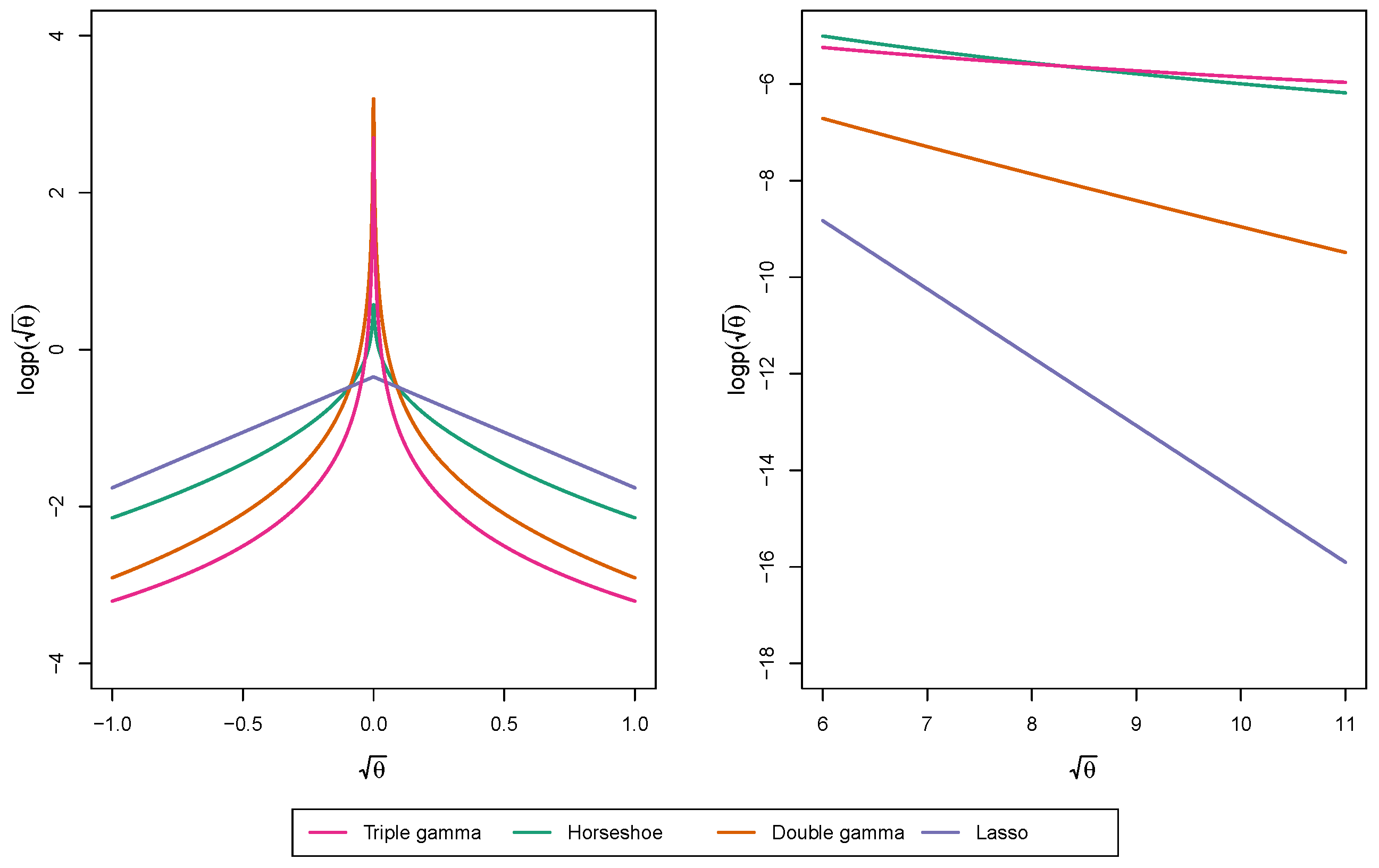
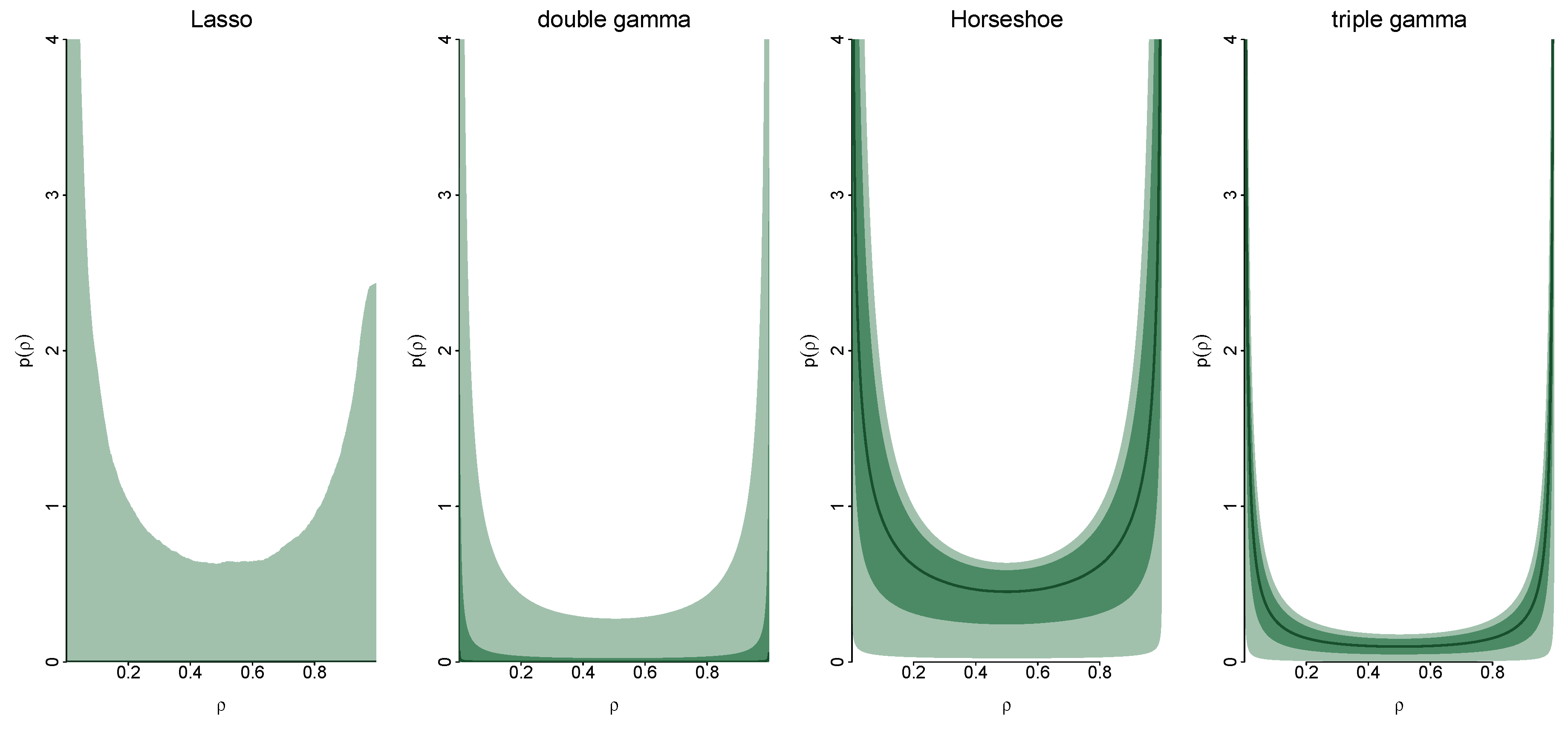
3. Shrinkage Profiles and BMA-Like Behavior

3.1. Shrinkage Profiles

In the sparse normal-means problem where y | β N d β , σ 2 I d and σ 2 = 1 , the parameter ρ j = 1 / ( 1 + ψ j 2 ) appearing in (14) is known as shrinkage factor and plays a fundamental role for comparing different shrinkage priors, as ρ j determines shrinkage toward 0.
Also in a variance selection context, it is evident from (14) that values of ρ j 0 will introduce no shrinkage on θ j , whereas values of ρ j 1 will introduce strong shrinkage of θ j toward 0. Hence, the prior p ( ρ j ) , also called shrinkage profile, will play an instrumental role in the behaviour of different shrinkage priors. Following Carvalho et al. (2010), shrinkage priors are often compared in terms of the prior they imply on ρ j , that is, how they handle shrinkage for small “observations” (in our case innovations) and how robust they are to large “observations”. Note that we ideally want a shrinkage profile that has a pole in zero (heavy tails to avoid over-shrinking signals) and a pole in one (spikiness to shrink noise). The Horseshoe prior, for example, implies ρ j B 1 / 2 , 1 / 2 which is a shrinkage profile that takes this much desired form of a “horseshoe”, see Figure 2.
For the triple gamma prior, the shrinkage profile is given by the three-parameter beta prior p ( ρ j ) provided in (15). For ϕ ξ = 1 , ρ j B c ξ , a ξ and κ B 2 = 2 c ξ / a ξ . Choosing small values a ξ < < 1 will put prior mass close to 1, choosing small values c ξ < < 1 will put prior mass close to 0, whereas values for both a ξ and c ξ smaller than one will induce the form of a horseshoe prior for ρ j . Evidently, for ϕ ξ = 1 , a symmetric triple gamma prior with a ξ = c ξ implies a Horseshoe prior for ρ j that is symmetric around 0.5. This is illustrated in Figure 2 for a symmetric triple gamma with a ξ = c ξ = 0.1 .
In Figure 2 we can also see the shrinkage profile for the Bayesian Lasso and the double gamma, which correspond to a triple gamma where c ξ .4 For the Bayesian Lasso with a ξ = 1 , it is clear that the shrinkage profile p ( ρ j ) converges to a constant for ρ j 1 , while there is no mass around ρ j = 0 . This means that this prior tends to over-shrink signals, while not shrinking the noise completely to zero. A double gamma prior with a ξ < 1 has the potential to shrink the noise completely to zero, as  p ( ρ j ) has a pole at ρ j = 1 , but p ( ρ j ) has also zero mass around ρ j = 0 , meaning the prior encourages over-shrinking of signals.
When we make κ B 2 random, we obtain a “prior density” of shrinkage profiles, see Figure 3. We can see that such hierarchical versions of the Lasso and the double gamma have shrinkage profiles that resemble the ones of the Horseshoe and the triple gamma. We have used κ B 2 G 0.01 , 0.01 for the Lasso and the double gamma, 2 / κ B 2 F 1 , 1 for the Horseshoe and 2 / κ B 2 F 0.2 , 0.2 for the triple gamma, see Section 2.4.

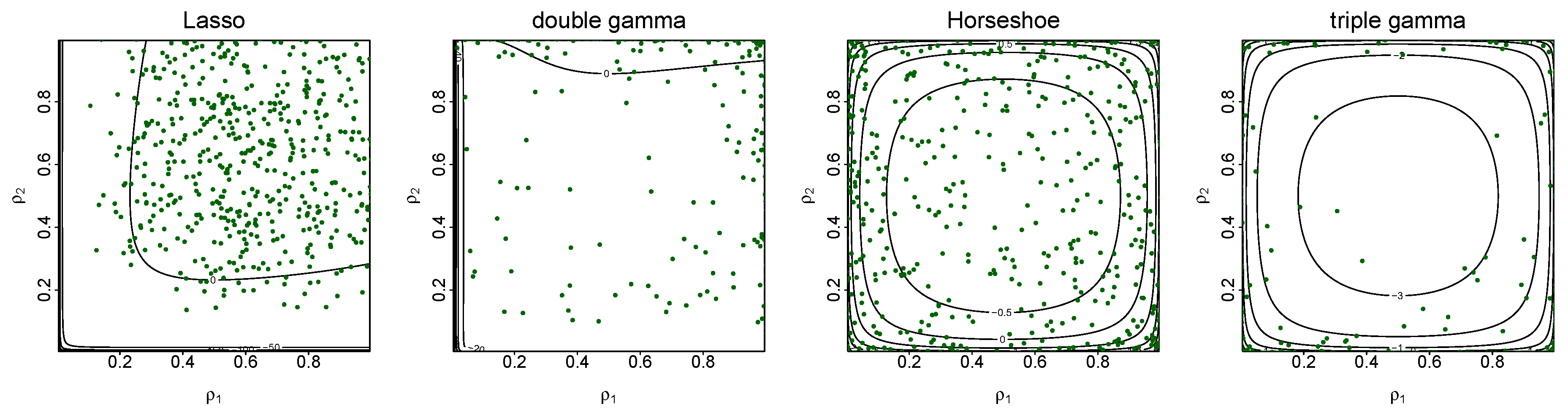
3.2. BMA-Type Behaviour

Bayesian model averaging (BMA) provides to statisticians and practitioners an essential and coherent tool to account for model uncertainty. In a multiple regression setting, the uncertainty is inherent in the choice of variables to be included. In a TVP framework, there is additional uncertainty about the time-variation of the state parameters, that is, which explanatory variables have a static and which ones a dynamic effect on the response variable. In this section, we show that the triple gamma prior mimics the typical BMA behavior, thus allowing us to incorporate model uncertainty with respect to time variation.
From the perspective of Bayesian model averaging, an ideal approach for handling sparsity in TVP models would be the use of discrete mixture priors as suggested in Frühwirth-Schnatter and Wagner (2010),
p ( θ j ) = ( 1 π ) δ 0 + π · p s l a b ( θ j ) ,
with δ 0 being a Dirac measure at 0, while p s l a b ( θ j ) is the prior for non-zero variances. In terms of shrinkage profiles, the discrete mixture prior (21) has a spike at ρ j = 1 , with probability 1 π , and a lot of prior mass at ρ j = 0 , provided that the tails of p slab ( θ j ) are heavy enough. The mixture prior (21) is considered the “gold standard” in BMA, both theoretically and empirically, see for example, Johnstone and Silverman (2004). However, MCMC inference under this prior is extremely challenging. As opposed to this, MCMC inference for the triple gamma prior is straightforward, see Section 4.
In this section, we relate the triple gamma prior to BMA based on the discrete mixture prior (21). An interesting insight is that the triple gamma prior shows a behaviour very similar to a discrete mixture prior, if both a ξ and c ξ approach zero. This induces BMA-type behaviour on the joint shrinkage profile p ( ρ 1 , , ρ d ) , with a spike at all corner solutions, where some ρ j are very close to one, whereas the remaining ones are very close to zero.
The bivariate shrinkage profiles shown in Figure 4 give us some intuition about the convergence of a symmetric triple gamma prior with a ξ = c ξ 0 toward a discrete spike and slab mixture. As opposed to the Lasso and the double gamma prior, the Horseshoe and the triple gamma prior put nearly all prior mass on the “corner solutions”, which correspond to the four possibilities (a) ρ 1 = ρ 2 = 0 , that is, no shrinkage on θ 1 and θ 2 , (b) ρ 1 = 1 , ρ 2 = 0 , that is, shrinkage of θ 1 toward 0 and no shrinkage on θ 2 , (c) ρ 1 = 0 , ρ 2 = 1 , that is, shrinkage of θ 1 toward 0 and no shrinkage on θ 2 , and (d) ρ 1 = ρ 2 = 1 , that is, shrinkage of both θ 1 and θ 2 toward 0.
A very important aspect of BMA is that of choosing a prior for the model dimension, K, see for example, Fernández et al. (2001) and Ley and Steel (2009). In the discrete mixture prior (21), the distribution of K depends on the choice of π . Fixing π corresponds to a very informative prior on the model dimension, for example π = 0.5 assigns more prior probability to models of dimension d / 2 and lower prior probability to empty or full models. In fact, let δ j be the indicator that tells us if the j-th coefficient is included in the model, then we have that K = j = 1 d δ j Binom d , π . Placing a uniform prior on π has been shown to be a good choice, since it corresponds to placing a prior on K which is uniform on { 0 , , d } . Note that π will be learned using information from all the variables. In this sense, π is a global shrinkage parameter which will adapt to the degree of sparsity.
Following ideas in Carvalho et al. (2009), we believe that a natural way to perform variable selection in the continuous shrinkage prior framework is though thresholding. Specifically, we say that when ( 1 ρ j ) > 0.5 , or ρ j < 0.5 , the variable is included, otherwise it is not. Notice that this classification via thresholding makes perfect sense in the case of a triple gamma of which the Horseshoe is a special case, but less so for a Lasso or double gamma prior, even if the shrinkage profile shows a Horseshoe-like behaviour for hierarchical versions of these priors (see again Figure 3). Notice that thresholding implies a prior on the model dimension K. Specifically,
K = j = 1 d I { ρ j < 0.5 } Binom d , π ξ , π ξ = Pr ( ρ j < 0.5 ) ,
where ρ j | a ξ , ϕ ξ TPB a ξ , b ξ , ϕ ξ , see (15). The choice of ϕ ξ (or κ B 2 ) will strongly impact the prior on K. For a symmetric triple gamma with a ξ = c ξ , for instance, and fixed ϕ ξ = 1 , that is κ B 2 = 2 , we obtain K Binom d , 0.5 , since π ξ = 0.5 regardless of a ξ . Hence, we have to face similar problems as with fixing π = 0.5 for the discrete mixture prior (21).
Placing a hyper prior on ϕ τ and ϕ ξ (or equivalent ones on λ B 2 and κ B 2 ), as we did in Section 2.4, is as vital for BMA-type variable and variance selection through the triple gamma prior, as making π random is for the discrete mixture prior (21). Ideally, we would like to have a uniform distribution on the model size K. We show in Theorem 3 that the hyperprior for κ B 2 defined in (17) achieves exactly this goal, since π ξ is uniformly distributed, see Appendix A for a proof.
Theorem 3.
For a hierarchical triple gamma prior with fixed a ξ > 0 and c ξ > 0 the probability π ξ defined in (22) follows a uniform distribution, π ξ U 0 , 1 , under the hyper prior
κ B 2 2 a ξ , c ξ F 2 a ξ , 2 c ξ ,
or, equivalently, under the hyper prior
ϕ ξ | a ξ , c ξ BP c ξ , a ξ .
Finally, it is important to point out that the thresholding approach allows us to estimate posterior inclusion probabilities, that is the probability that the corresponding variable is included in the model or, in the case of variance selection, that the corresponding parameter is time varying. In our simulations (Section 5.3) and in our application (Section 5.4), we will estimate the posterior inclusion probabilities obtained under different shrinkage priors.

4. MCMC Algorithm

Let y = ( y 1 , , y T ) be the vector of time series observations and let z be the set of all latent variables and unknown model parameters in a TVP model. Moreover, let z x denote the set of all unknowns but x. Bayesian inference based on MCMC sampling from the posterior p ( z | y ) is summarized in Algorithm 1. The hierarchical priors introduced in Section 2.4 are employed, where κ B 2 follows (17), ( a ξ , c ξ ) follow (19), and ( a τ , c τ , λ B 2 ) follow (20). For certain sampling steps, the hierarchical representation (18) is used for κ B 2 , and similarly for λ B 2 .
Algorithm 1 extends several existing algorithms such as the MCMC schemes introduced for the Horseshoe prior by Makalic and Schmidt (2016) and for the double gamma prior by Bitto and Frühwirth-Schnatter (2019). We exploit various representations of the triple gamma prior given in Lemma 1 and choose representation (12) as the baseline representation of our MCMC algorithm:
β j | τ ˇ j 2 , λ ˇ j 2 , ϕ τ N 0 , ϕ τ τ ˇ j 2 / λ ˇ j 2 , τ ˇ j 2 | a τ G a τ , 1 , λ ˇ j 2 | c τ G c τ , 1 , θ j | ξ ˇ j 2 , κ ˇ j 2 , ϕ ξ N 0 , ϕ ξ ξ ˇ j 2 / κ ˇ j 2 , ξ ˇ j 2 | a ξ G a ξ , 1 , κ ˇ j 2 | c ξ G c ξ , 1 ,
where ϕ τ = 2 c τ / ( λ B 2 a τ ) and ϕ ξ = 2 c ξ / ( κ B 2 a ξ ) . All conditional distributions in our MCMC scheme are available in closed form, except for the ones for a ξ , c ξ , a τ and c τ , for which we will resort to a Metropolis-Hastings (MH) step within Gibbs. Several conditional distributions are the same as for the double gamma prior and we apply Algorithm 1 of Bitto and Frühwirth-Schnatter (2019). We provide more details on the derivation of the various densities in Appendix B.
Algorithm 1. MCMC inference for TVP models under the triple gamma prior.
Choose starting values for all global shrinkage parameters ( a τ , c τ , λ B 2 , a ξ , c ξ , κ B 2 ) and local shrinkage parameters { τ ˇ j 2 , λ ˇ j 2 , ξ ˇ j 2 , κ ˇ j 2 } j = 1 d , and repeat the following steps:
(a) 
Define for j = 1 , , d , τ j 2 = ϕ τ τ ˇ j 2 / λ ˇ j 2 and ξ j 2 = ϕ ξ ξ ˇ j 2 / κ ˇ j 2 and sample from the posterior p ( β ˜ 0 , , β ˜ T , β 1 , , β d , θ 1 , , θ d | { ξ j 2 , τ j 2 } j = 1 d , y ) using Algorithm 1, Steps (a), (b), and (c) in Bitto and Frühwirth-Schnatter (2019). In the homoscedastic case, use Step (f) of this algorithm to sample from σ 2 | z σ 2 , y . For the SV model (2), sample the parameters μ, ϕ, and σ η 2 as in Kastner and Frühwirth-Schnatter (2014), for example, using the R-packagestochvol(Kastner 2016).
(b) 
Use the prior p ( θ j | κ ˇ j 2 , a ξ , c ξ ) , marginalized w.r.t. ξ ˇ j 2 , to sample a ξ from p ( a ξ | z a ξ , y ) via a random walk MH step on z = log ( a ξ / ( 0.5 a ξ ) ) . Propose a ξ , ( * ) = 0.5 e z * / ( 1 + e z * ) , where z * N z ( m 1 ) , v 2 and z ( m 1 ) = log ( a ξ , ( m 1 ) / ( 0.5 a ξ , ( m 1 ) ) ) depends on the previous value a ξ , ( m 1 ) of a ξ , accept a ξ , ( * ) with probability
min 1 , q a ( a ξ , ( * ) ) q a ( a ξ , ( m 1 ) ) , q a ( a ξ ) = p ( a ξ | z a ξ , y ) a ξ ( 0.5 a ξ ) ,
and update ϕ ξ = 2 c ξ / ( κ B 2 a ξ ) . Explicit forms for p ( a ξ | z a ξ , y ) and log q a ( a ξ ) are provided in (A3) and (A4).
Similarly, use the prior p ( β j | λ ˇ j 2 , a τ , c τ ) , marginalized w.r.t. to τ ˇ j 2 , to sample a τ via a random walk MH step and update ϕ τ = 2 c τ / ( a τ λ B 2 ) .
(c) 
Sample ξ ˇ j 2 , j = 1 , , d , from a generalized inverse Gaussian distribution, see (A5):
ξ ˇ j 2 | κ ˇ j 2 , θ j , a ξ , ϕ ξ GIG a ξ 1 2 , 2 , κ ˇ j 2 θ j ϕ ξ .
Similarly, update τ ˇ j 2 , j = 1 , , d , conditional on a τ :
τ ˇ j 2 | β j , λ ˇ j 2 , a τ , ϕ τ GIG a τ 1 2 , 2 , λ ˇ j 2 β j 2 ϕ τ .
(d) 
Use the marginal Student-t distribution p ( θ j | ξ ˇ j 2 , c ξ , κ B 2 ) given in (11) to sample c ξ from p ( c ξ | z c ξ , y ) via a random walk MH step on z = log ( c ξ / ( 0.5 c ξ ) ) . Propose c ξ , ( * ) = 0.5 e z * / ( 1 + e z * ) , where z * N z ( m 1 ) , v 2 and z ( m 1 ) = log ( c ξ , ( m 1 ) / ( 0.5 c ξ , ( m 1 ) ) ) depends on the previous value c ξ , ( m 1 ) of c ξ , accept c ξ , ( * ) with probability
min 1 , q c ( c ξ , ( * ) ) q c ( c ξ , ( m 1 ) ) , q c ( c ξ ) = p ( c ξ | z c ξ , y ) c ξ ( 0.5 c ξ ) ,
and update ϕ ξ = 2 c ξ / ( κ B 2 a ξ ) . Explicit forms for p ( c ξ | z c ξ , y ) and log q c ( c ξ ) are provided in (A6) and (A7).
Similarly, to sample c τ via a random walk MH step use the marginal distribution of β j | τ ˇ j 2 , a τ , c τ with respect to λ ˇ j 2 and update ϕ τ = 2 c τ / ( a τ λ B 2 ) .
(e) 
Sample κ ˇ j 2 , for j = 1 , , d , from following gamma distribution, see (A8):
κ ˇ j 2 | θ j , ξ ˇ j 2 , c ξ , ϕ ξ G 1 2 + c ξ , θ j 2 ϕ ξ ξ ˇ j 2 + 1 .
Similarly, update λ ˇ j 2 , j = 1 , , d , conditional on c τ :
λ ˇ j 2 | β j , τ ˇ j 2 , c τ , ϕ τ G 1 2 + c τ , β j 2 2 ϕ τ τ ˇ j 2 + 1 .
(f) 
Sample d 2 from d 2 | a ξ , c ξ , κ B 2 G a ξ + c ξ , κ B 2 + 2 c ξ a ξ , see (A9); sample from κ B 2 from following gamma distribution,
κ B 2 | { θ j , κ ˇ j 2 , ξ ˇ j 2 } j = 1 d , a ξ , c ξ , d 2 G d 2 + a ξ , a ξ 4 c ξ j = 1 d κ ˇ j 2 ξ ˇ j 2 θ j + d 2 ,
see (A10), and update ϕ ξ = 2 c ξ / ( κ B 2 a ξ ) .
Similarly, sample e 2 from e 2 | a τ , c τ , λ B 2 G a τ + c τ , λ B 2 + 2 c τ a τ , sample λ B 2 from
λ B 2 | { β j , λ ˇ j 2 , τ ˇ j 2 } j = 1 d , a τ , c τ , e 2 G d 2 + a τ , a τ 4 c τ j = 1 d λ ˇ j 2 τ ˇ j 2 β j 2 + e 2 ,
and update ϕ τ = 2 c τ / ( a τ λ B 2 ) .
The MCMC scheme in Algorithm 1 is not a full conditional scheme, as several steps are based on partially marginalized distributions. That means that the sampling order matters. For instance, in Step (b), we marginalize w.r.t. ξ ˇ 1 2 , , ξ ˇ d 2 , hence we need to update ξ ˇ 1 2 , , ξ ˇ d 2 after sampling a ξ , before we update c ξ in Step (d) conditional on ξ ˇ 1 2 , , ξ ˇ d 2 . Similarly, due to marginalization in Step (d), we need to update κ ˇ 1 2 , , κ ˇ d 2 , before we update d 2 in Step (f). Furthermore, both Step (b) and Step (d) are based on the marginal prior of κ B 2 , given in (17). Hence, in Step (f), d 2 has to be updated from d 2 | a ξ , c ξ , κ B 2 , before κ B 2 is updated conditional on d 2 .
For a symmetric triple gamma prior, where a ξ = c ξ , the MCMC scheme in Algorithm 1 has to be modified only slightly. Either q a ( a ξ ) in Step (b) is adjusted and Step (d) is skipped, setting c ξ = a ξ , or q c ( c ξ ) in Step (d) is adjusted and Step (b) is skipped, setting a ξ = c ξ . In Appendix B, we provide details in (A11) for the first case and in (A12) for the second case. Similar modifications are needed, if a τ = c τ . All other steps in Algorithm 1 remain the same for a ξ = c ξ and/or a τ = c τ .

5. Applications to TVP-VAR-SV Models

5.1. Model

In this section, we consider a generalization of the TVP model (1), where y t is a m-dimensional time series, observed for t = 1 , , T . The time series y t is assumed to follow a time-varying parameter vector autoregressive model with stochastic volatility (TVP-VAR-SV) of order p:
y t = c t + Φ 1 , t y t 1 + Φ 2 , t y t 2 + Φ p , t y t p + ε t , ε t N m 0 , Σ t ,
where c t is the m-dimensional time-varying intercept, Φ j , t , for j = 1 , , p is an m × m matrix of time-varying coefficients, and Σ t is the time-varying variance covariance matrix of the error term. The TVP-VAR-SV model can be written in a more compact notation as the following TVP model:
y t = ( I m x t ) β t + ε t , ε t N m 0 , Σ t ,
where x t = ( y t 1 , , y t p , 1 ) is a row vector of length m p + 1 and the time-varying parameter β t is defined as β t = ( β t 1 , , β t m ) , where β t i = ( Φ 1 , t i , , Φ p , t i , c t , i ) . Here, Φ j , t i denotes the i-th row of the matrix Φ j , t and c t , i denotes the i-th element of c t . Since the influential paper of Primiceri (2005) (see Del Negro and Primiceri (2015) for a corrigendum), this model has become a benchmark for analyzing relationships between macroeconomic variables that evolve over time, see Nakajima (2011), Koop and Korobilis (2013), Eisenstat et al. (2014), Chan and Eisenstat (2016), Feldkircher et al. (2017) and Carriero et al. (2019), among many others.
Following Frühwirth-Schnatter and Tüchler (2008), we use a Cholesky decomposition of the time-varying covariance matrix Σ t , that is Σ t = A t D t A t , where D t is a diagonal matrix and A t is lower unitriangular matrix, see Carriero et al. (2019) and Bitto and Frühwirth-Schnatter (2019) for related models. We denote with a i j , t the element at the i-th row and j-th column of A t , and with σ i , t 2 the i-th diagonal element of D t = Diag σ 1 , t 2 σ m , t 2 . In total, we have m ( m 1 ) / 2 + m ( m p + 1 ) (potentially) time-varying parameters. Using the Cholesky decomposition, we can rewrite the system as:
y t = ( I m x t ) β t + A t η t , η t N m 0 , D t ,
where η t = ( η 1 , t , , η m , t ) . The idiosyncratic shocks η i , t N 0 , σ i , t 2 follow independent SV processes as in (2), with row specific parameters. Specifically, with h i , t = log σ i , t 2 , we have that the logarithm of the elements of the diagonal matrix D t follow independent AR(1) processes:
h i , t = μ i + ϕ i ( h i , t 1 μ i ) + ν i , t , ν i , t N 0 , σ η , i 2 ,
for i = 1 , , m . Here, μ i is the mean, ϕ i is the persistence parameter, and σ η , i 2 is the variance of the ith log-volatility h i , t .
It is possible to write the TVP-VAR-SV model (30) as a system of m univariate TVP models as in (1):
y 1 , t = x t β t 1 + η 1 , t , η 1 , t N 0 , σ 1 , t 2 , y 2 , t = x t β t 2 + a 21 , t η 1 , t + η 2 , t , η 2 , t N 0 , σ 2 , t 2 , y 3 , t = x t β t 3 + a 31 , t η 1 , t + a 32 , t η 2 , t + η 3 , t , η 3 , t N 0 , σ 3 , t 2 , y m , t = x t β t m + a m 1 , t η 1 , t + + a m , m 1 , t η m 1 , t + η m , t , η m , t N 0 , σ m , t 2 .
Note that for i > 1 , the i-th equation of this system is a TVP model where the residuals of the preceding i 1 equations are added as explanatory variables:
y i , t = x t β t i + j = 1 i 1 a i j , t η j , t + η i , t , η i , t N 0 , σ i , t 2 ,
and all time-varying parameters follow a random walk as in the TVP model (1):
β j , t i = β j , t 1 i + v i j , t , v i j , t N 0 , θ i j β , for i = 1 , , m , and j = 1 , , m p + 1 , a i j , t = a i j , t 1 + w i j , t , w i j , t N 0 , θ i j a , for i = 1 , , m , and j = 1 , , i 1 ,
with initial values β j , 0 i N β i j β , θ i j β and a i j , 0 N β i j a , θ i j a . Here, β j , t i denotes the jth element of the vector β t i .
To achieve shrinkage for each VAR coefficient β j , t i as well as for each Cholesky factor a i j , t , we proceed as in Section 2 and introduce shrinkage priors for the initial expectations β i j β and β i j a as well as the variances θ i j β and θ i j a . We do this independently for each equation of the system. Within each equation, the β i j β s and β i j a s are assumed to follow independent shrinkage priors to allow for flexibility in the prior structure, and similarly for θ i j β and θ i j a :
β i j x N 0 , ϕ i τ , x τ ˇ i j x , 2 / λ ˇ i j x , 2 , τ ˇ i j x , 2 G a i τ , x , 1 , λ ˇ i j x , 2 G c i τ , x , 1 , ϕ i τ , x = 2 c i τ , x / ( λ B , i x , 2 a i τ , x ) , θ i j x N 0 , ϕ i ξ , x ξ ˇ i j x , 2 / κ ˇ i j x , 2 , ξ ˇ i j x , 2 G a i ξ , x , 1 , κ ˇ i j x , 2 G c i ξ , x , 1 , ϕ i ξ , x = 2 c i ξ , x / ( κ B , i x , 2 a i ξ , x ) ,
where x = β for the VAR-coefficients and x = a for the elements of A t . Following Section 2.4, the priors for the global shrinkage parameters in the ith equation read
λ B , i x , 2 | a i τ , x , c i τ , x F 2 a i τ , x , 2 c i τ , x , 2 a i τ , x B α a τ , β a τ , 2 c i τ , x B α c τ , β c τ , κ B , i x , 2 | a i ξ , x , 2 c i ξ , x F 2 a i ξ , x , 2 c i ξ , x , 2 a i ξ , x B α a ξ , β a ξ , 2 c i ξ , x B α c ξ , β c ξ .

5.2. A Brief Sketch of the TVP-VAR-SV MCMC Algorithm

Our algorithm exploits the aforementioned unitriangular decomposition to estimate the model parameters equation-by-equation. Due to the prior structure introduced in (31), the estimation of β t i and the a i j , t ’s is separated into two blocks, with the algorithm cycling through the m equations, alternating between sampling β t i conditional on Σ t and sampling the a i j , t s and d i , t s conditional on the VAR coefficients β t i . Given a set of initial values, the algorithm repeats the following steps:
Algorithm 2. MCMC inference for TVP-VAR-SV models under the triple gamma prior.
Choose starting values for all global and local shrinkage parameters in prior (31) for each equation and repeat the following steps:
For i = 1 , , m , update all the unknowns in the ith equation:
(a) 
Conditional on A t and D t , create y ˇ i , t = y i , t j = 1 i 1 a i j , t η j , t and define the following TVP model:
y ˇ i , t = x t β t i + η i , t , η i , t N 0 , σ i , t 2 .
Apply Algorithm 1 (sans the step for the variance of the observation equation) to this univariate TVP model, to draw from the conditional posterior distribution of the time-varying VAR-coeffcients β t i , for t = 0 , , T , their initial expectations β i j β , the process variances θ i j β , the local shrinkage parameters τ ˇ i j β , 2 , λ ˇ i j β , 2 , ξ ˇ i j β , 2 , κ ˇ i j β , 2 , as well as the global shrinkage parameters λ B , i β , 2 , κ B , i β , 2 , a i τ , β , c i τ , β , a i ξ , β , and c i ξ , β .
(b) 
For i > 1 , create y i , t 🟉 = y i , t x t β t i , conditional on β t i , and define the following TVP model:
y i , t 🟉 = j = 1 i 1 a i j , t η j , t + η i , t , η i , t N 0 , σ i , t 2 ,
where the residuals from the previous i 1 equations, ( η 1 , t , , η i 1 , t ) , are used as explanatory variables and no intercept is present. Apply Algorithm 1 to this univariate TVP model, to sample the volatilities σ i , t 2 and the time-varying coefficients a i j , t in the ith row of A t for t = 0 , , T from the respective conditional posteriors, as well as the initial expectations β i j a , the process variances θ i j a , the local shrinkage parameters τ ˇ i j a , 2 , λ ˇ i j a , 2 , ξ ˇ i j a , 2 , κ ˇ i j a , 2 and the global shrinkage parameters λ B , i a , 2 , κ B , i a , 2 , a i τ , a , c i τ , a , a i ξ , a , and c i ξ , a .
In the following applications, we run our algorithm for M = 200 , 000 iterations, discarding the first 100 , 000 iterations as burn-in, and then keeping the output of one every 100 iterations.

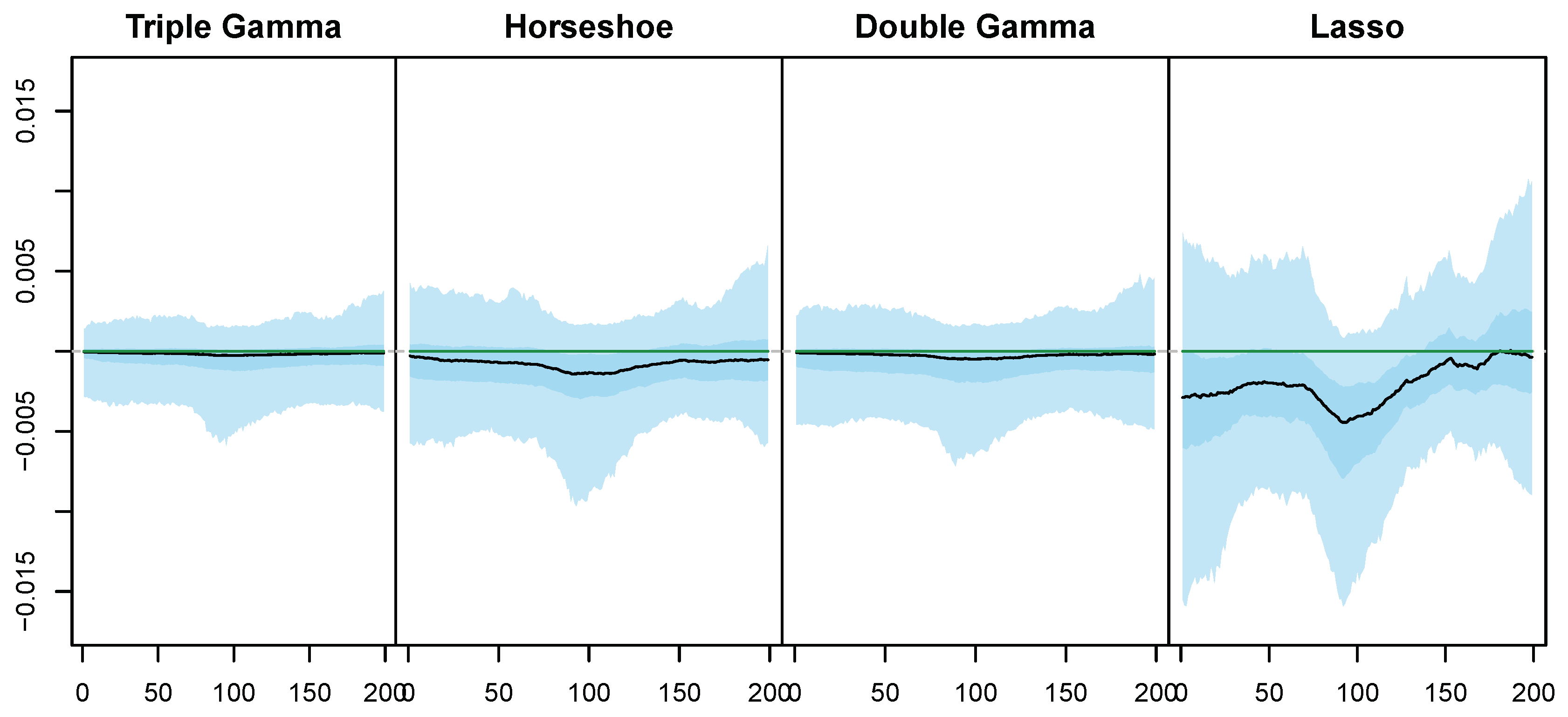
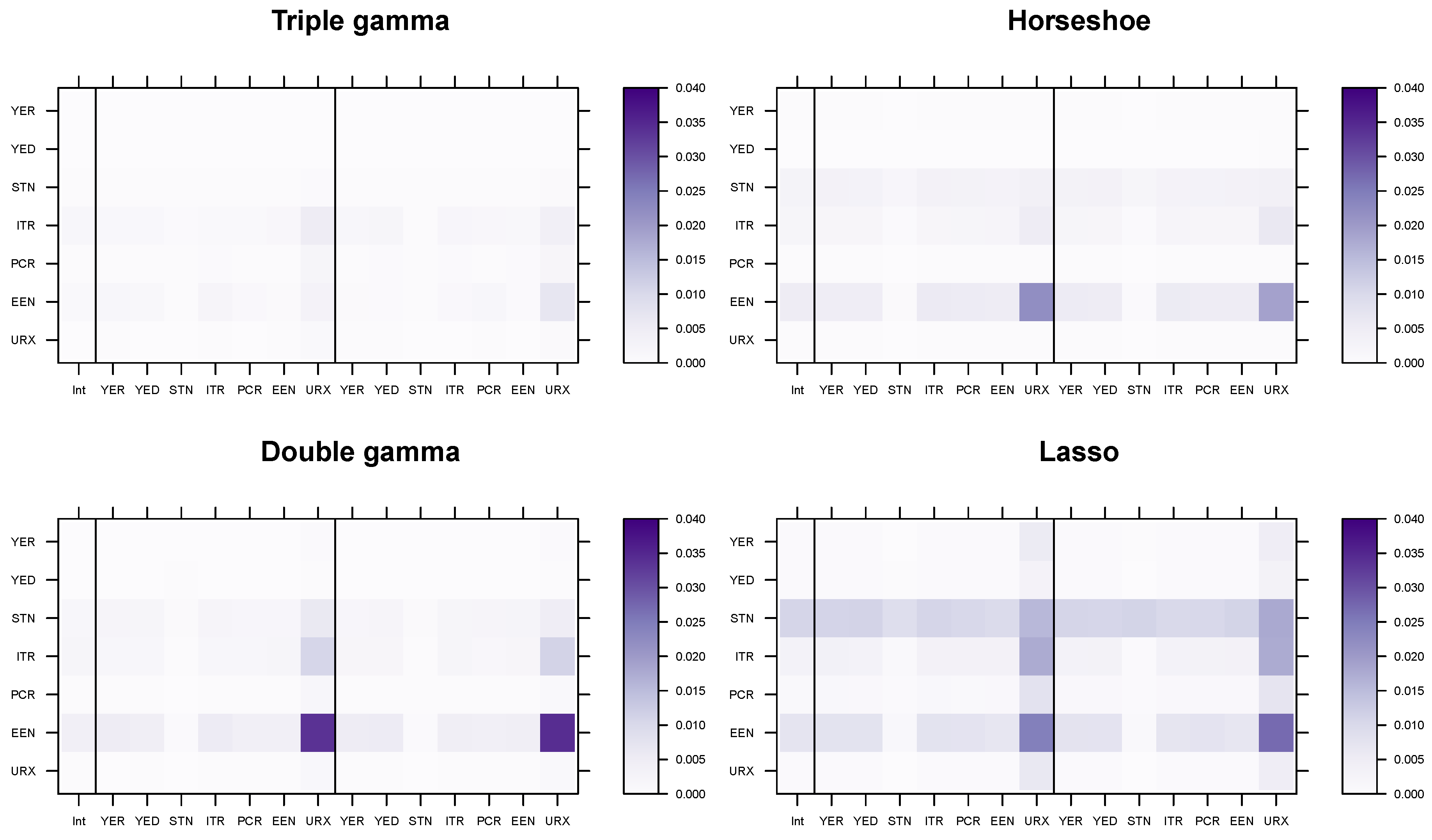
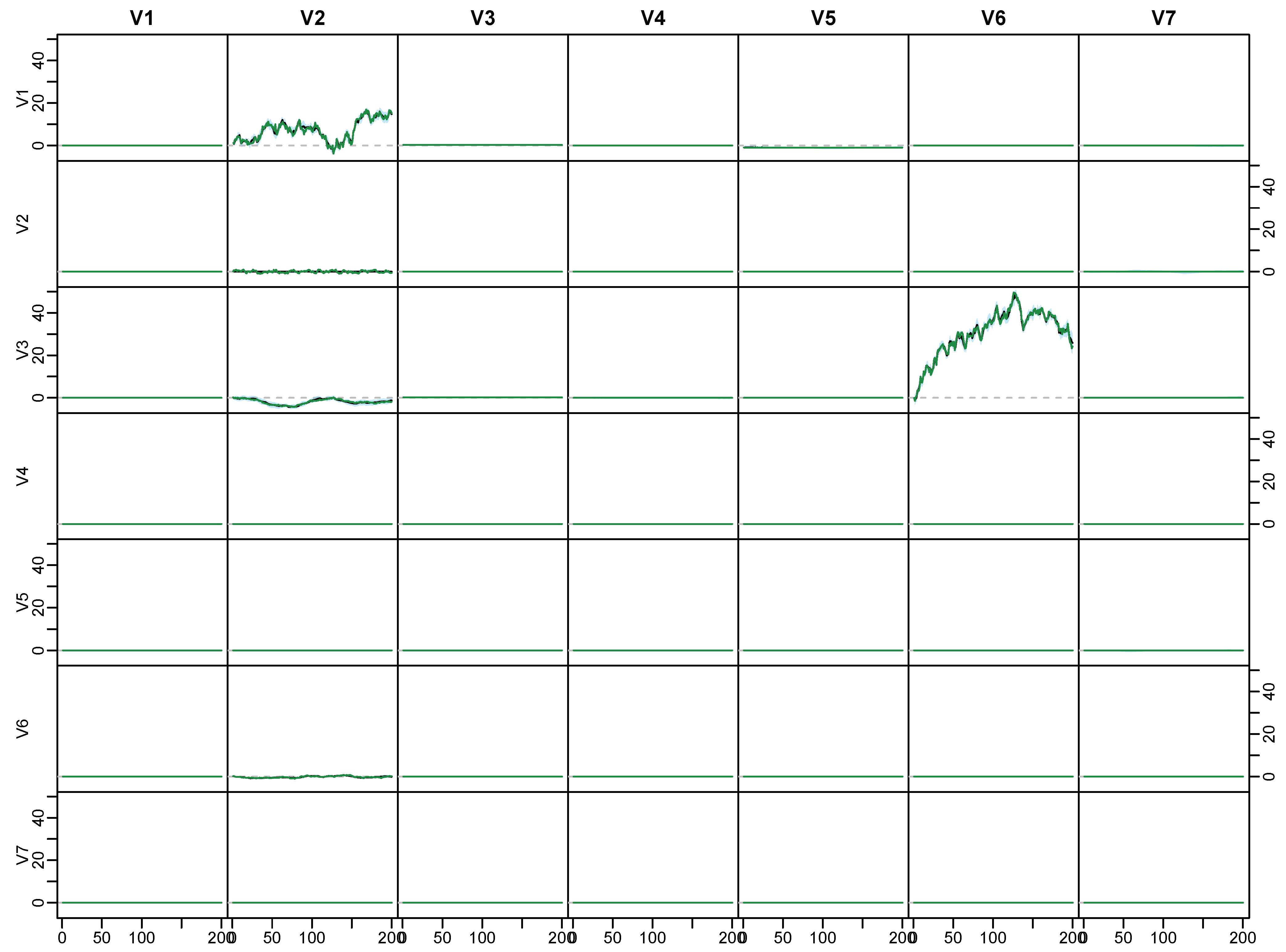
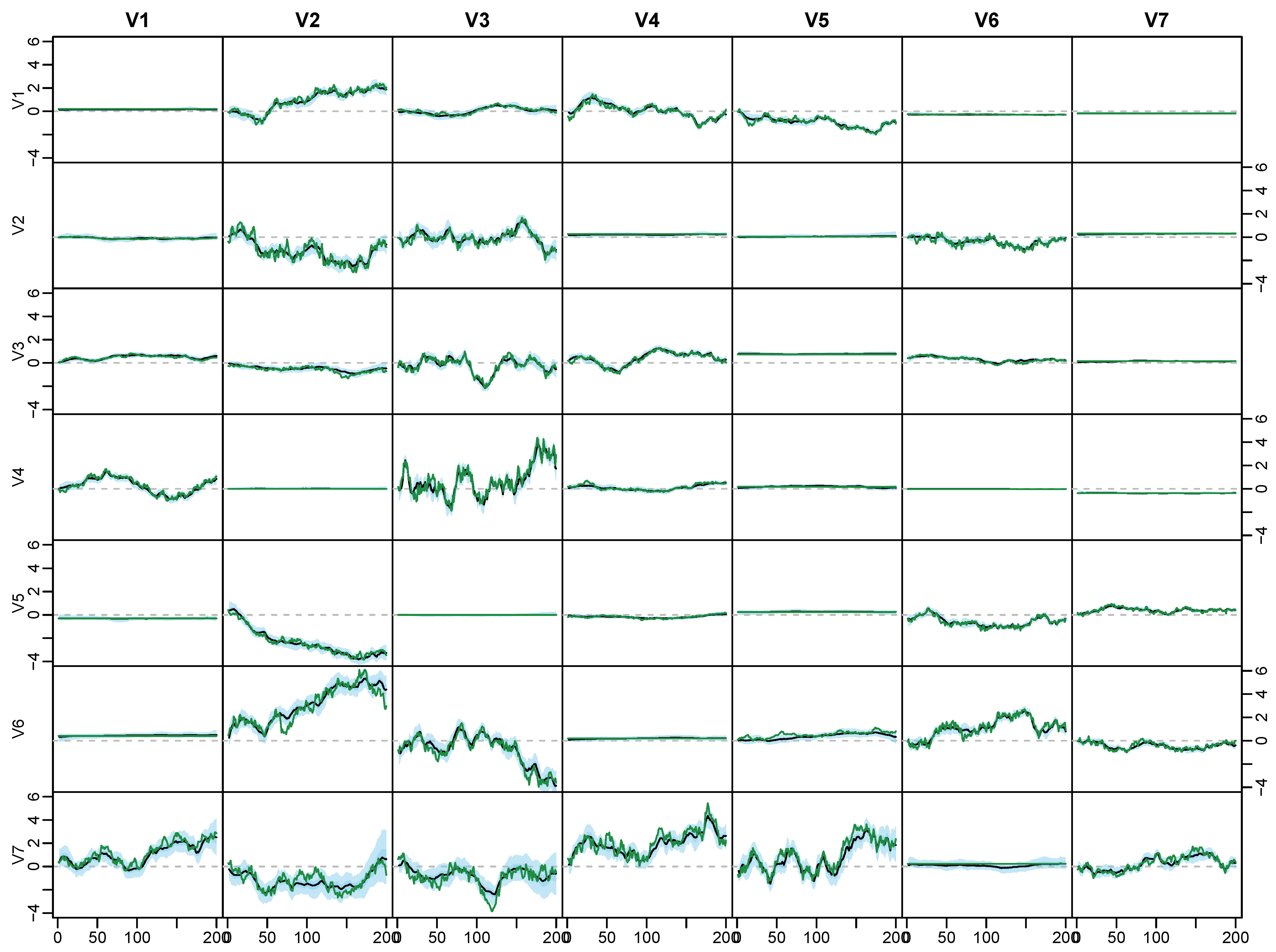
5.3. Illustrative Example with Simulated Data

To illustrate the merit of our methodology in the context of TVP-VAR-SV models, we simulate data from two TVP-VAR-SV models with T = 200 points in time, p = 1 lags and m = 7 equations, with varying degrees of sparsity. In the dense regime, approximately 30% of the values of β and θ (here referring to the means of the initial states and the variances of the innovations as defined in Section 2, respectively) are truly zero, while in the sparse regime approximately 90% are truly zero. We show results for the triple gamma prior, the Horseshoe prior, the double gamma and the Lasso.
Regarding the priors on the hyperparameters, we use prior (32) with α a τ = α c τ = α a ξ = α c ξ = 1 and β a τ = β c τ = β a ξ = β c ξ = 6 for the triple gamma. The probability density function of the corresponding beta prior is monotonically increasing, with a maximum at 0.5 . This prior places positive mass in a neighborhood of the Horseshoe, but allows for more flexibility. In practice, placing a prior on the spike and slab parameters of the triple gamma, instead of fixing them to 0.5 as in the Horseshoe, allows us to learn the shrinkage profile from the data, including asymmetric profiles.
We assume that the global shrinkage parameters λ B , i β , 2 , κ B , i β , 2 , λ B , i a , 2 , and κ B , i a , 2 follow a F 1 , 1 distribution for the Horseshoe prior which corresponds to the prior in Carvalho et al. (2009) and a G 0.001 , 0.001 distribution for the Lasso and the double gamma prior, as suggested in Belmonte et al. (2014) and Bitto and Frühwirth-Schnatter (2019). Concerning the spike parameters a i τ , a , a i ξ , a , a i τ , β , and a i ξ , β of the double gamma, we employ a rescaled beta prior to force them to be smaller than 0.5 . Specifically, we use a B ( 4 , 6 ) prior which places most of its mass between 0.05 and 0.4 , a range that Bitto and Frühwirth-Schnatter (2019) have found to induce desirable shrinkage characteristics.
Figure 5 shows the posterior path of a permanently non-significant state, that is a state where the true β j , t i = 0 for t = 1 , , T , in the sparse regime. The entire set of states for the triple gamma prior can be found in Appendix C. Note that, while the zero line is contained in the 95% posterior credible interval for all priors, said interval is thinner under the triple gamma prior and the double gamma prior than under the Lasso and the Horseshoe prior.
We calculate the posterior inclusion probabilities based on the thresholding approach introduced in Section 3.2, comparing the triple gamma prior to widely used special cases. In a variance selection context, the posterior inclusion probabilities reflect the uncertainty on whether a state should be time varying or constant over time. Figure 6 shows the posterior inclusion probabilities for the variance of the innovations ( θ i j β ’s) under four different shrinkage priors, for the sparse and the dense scenario, respectively. The cells are shaded in gray when the corresponding true state parameter is time-varying ( θ i j β 0 ), while the background is white when the corresponding true state parameter is not time-varying ( θ i j β = 0 ). In this simulated example, the posterior inclusion probabilities under the triple gamma prior are consistently higher for the variances that are actually different from 0, even when they are very small. This outcome is in line with the analytical results derived in Section 2.2, which show that the tails of the triple gamma prior are heavier than those of the other priors.

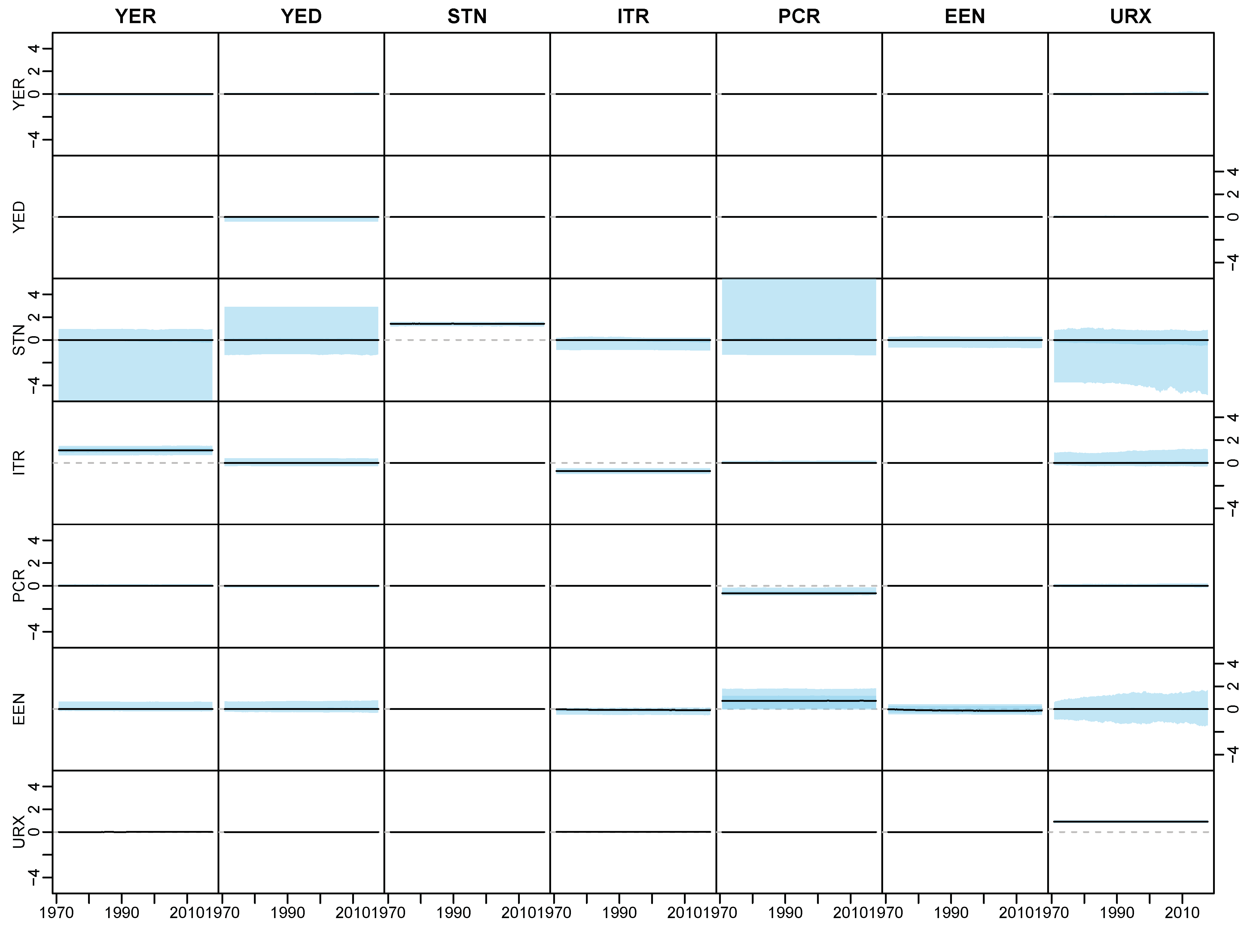
5.4. Modeling Area Macroeconomic and Financial Variables in the Euro Area

Our application investigates a subset of the area wide model of the European Union of Fagan et al. (2005), which comprises quarterly macroeconomic data spanning from 1970 to 2017. We include seven of the variables present in the dataset, namely real output (YER), prices (YED), short-term interest rate (STN), investment (ITR), consumption (PCR), exchange rate (EEN) and unemployment (URX). A more detailed description of the data and the transformations performed to make the time series stationary can be found in Table A1 in Appendix D. To stay in line with the literature, for example, Feldkircher et al. (2017), we estimate a TVP-VAR-SV model with p = 2 lags on all endogenous variables. The hyperparameter choices are the same as in Section 5.3. As in the example with simulated data, we run the algorithm for M = 200,000 iterations, discarding the first 100,000 iterations as burn-in, and then keeping the output of one every 100 iterations.
Figure 7 and Figure 8 display the posterior inclusion probabilities for the means of the initial states and the innovation variances of the VAR coefficients, respectively. A few things about Figure 7 are noteworthy. First, the posterior inclusion probabilities on the diagonal, meaning those belonging to the parameter of each equation’s own autoregressive term, appear to be those that are the highest, while off diagonal elements are more likely to be excluded. Second, the equation for the short-term interest rate is characterized by a large amount of parameters with a high inclusion probability, across all priors. Third, the first lag tends to have higher posterior inclusion probabilities than the second lag, which is in line with the literature. In most cases, the triple gamma prior can be seen to have either the largest or the smallest posterior inclusion probability compared to the other priors. This can be seen as a reflection of the fact that the triple gamma prior places more mass on the edges of the shrinkage profile, as illustrated in Section 3.
Now, we shift our focus to the posterior inclusion probabilities for the θ i j β ’s plotted in Figure 8. Compared to the means of the inital states, almost all inclusion probabilities are essentially zero. This lack of variability is unsurprising, as it is well known (see, e.g., Feldkircher et al. (2017)) that stochastic volatility in a TVP-VAR model for macroeconomic variables can explain a large part of the variability in the data. However, the triple gamma prior appears to allow posterior distributions that place slightly more mass on models with some time variation, in particular with respect to the financial variables.
Figure 9 and Figure 10 display the posterior median of β i j β and θ i j β , respectively. Here the triple gamma can be seen to be quite conservative, both in terms of which parameters to include, as well as their magnitude. In particular the medians of the θ i j β are interesting, as they are closest to zero under the triple gamma prior, despite having the highest posterior inclusion probabilities among all considered priors.
In Figure A3 and Figure A4 in Appendix D, all the posterior paths of Φ 1 , t and Φ 2 , t under the triple gamma prior are shown.

6. Conclusions

In the present paper, shrinkage for time-varying parameter (TVP) models was investigated within a Bayesian framework with the goal to automatically reduce time-varying parameters to static ones, if the model is overfitting. This goal was achieved by suggesting the triple gamma prior as a new shrinkage priors for the process variances of varying coefficients, extending previous work using spike-and-slab priors, the Bayesian Lasso, or the double gamma prior. The triple gamma prior is related to the normal-gamma-gamma prior applied for variable selection in highly structured regression models (Griffin and Brown 2017). It contains the well-known Horseshoe prior as a special case, however it is more flexible, with two shape parameters that control concentration at zero and the tail behaviour. This leads to a BMA-type behaviour which allows not only variance shrinkage, but also variance selection.
In our application, we considered time-varying parameter VAR models with stochastic volatility. Overall, our findings suggest that the family of triple gamma priors introduced in this paper for sparse TVP models is successful in avoiding overfitting, if coefficients are, indeed, static or even insignificant. The framework developed in this paper is very general and holds the promise to be useful for introducing sparsity in other TVP and state space models in many different settings.
A number of extensions seem to be worth pursuing. First of all, the triple gamma prior is relevant not only for TVP models, but for any model containing variance parameters such as random-effect models or Bayesian p-splines models (Scheipl and Kneib 2009). Second, in particular, in ultra-sparse settings, modifications of the triple gamma prior seem sensible. Currently, the hyperprior for the global shrinkage parameter of the triple gamma prior is selected in a way that it implies a uniform prior on “model size”. A generalization of Theorem 3 would allow the choice of hyper priors that induce higher sparsity. Furthermore, in the variable selection literature, special priors such as the Horseshoe+ (Bhadra et al. 2017a) were suggested for very sparse, ultra-sparse high dimensional settings. Exploiting once more the non-centered parametrization of a state space model, it is straightforward to extend this prior to variance selection using following hierarchical representation:
θ j | κ j 2 , ξ j 2 N 0 , 2 κ B 2 κ j 2 ξ j 2 , κ j t 1 , ξ j t 1 .
We leave these extensions for future research.
Finally, an important limitation of our approach is that shrinking a variance toward zero implies that a coefficient is fixed over the entire observation period of the time series. In future research we will investigate dynamic shrinkage priors (Kalli and Griffin 2014; Kowal et al. 2019; Ročková and McAlinn 2020) where coefficients can be both fixed and dynamic.

Author Contributions

The authors contributed equally to the work. All authors have read and agreed to the published version of the manuscript.

Conflicts of Interest

The authors declare that there is no conflict of interest.

Appendix A. Proofs

Proof of Theorem 1.
To proof Part (a), rewrite prior (6) in the following way by rescaling ξ j 2 and κ j 2 :
θ j | ξ ˜ j 2 , κ ˜ j 2 , κ B 2 N 0 , 2 κ B 2 ξ ˜ j 2 κ ˜ j 2 , ξ ˜ j 2 | a ξ G a ξ , a ξ , κ ˜ j 2 | c ξ G c ξ , c ξ ,
and use the fact that in (A1) the random variable ψ j 2 = ξ ˜ j 2 / κ ˜ j 2 follows the F-distribution:
ψ j 2 = ξ ˜ j 2 κ ˜ j 2 G a ξ , a ξ G c ξ , c ξ = d F 2 a ξ , 2 c ξ ,
where p ( ψ j 2 ) is given by:
p ( ψ j 2 ) = 1 B ( a ξ , c ξ ) a ξ c ξ ψ j 2 a ξ 1 1 + a ξ c ξ ψ j 2 ( a ξ + c ξ ) .
This yields (8).
Using that η j = 1 / ψ j 2 F 2 c ξ , 2 a ξ , we obtain from (8) that
p ( θ j | κ B 2 , a ξ , c ξ ) = κ B 2 ( c ξ ) c ξ 4 π ( a ξ ) c ξ B ( a ξ , c ξ ) 0 exp θ j κ B 2 η j 4 η j c ξ 1 2 1 + c ξ η j a ξ ( a ξ + c ξ ) d η j .
A change of variable with y j = c ξ η j / a ξ proves Part (b):
p ( θ j | ϕ ξ , a ξ , c ξ ) = 1 2 π ϕ ξ B ( a ξ , c ξ ) 0 exp θ j 2 ϕ ξ y j y j c ξ 1 2 1 + y j ( a ξ + c ξ ) d y j = Γ ( c ξ + 1 2 ) 2 π ϕ ξ B ( a ξ , c ξ ) U c ξ + 1 2 , 3 2 a ξ , θ j 2 ϕ ξ ,
where ϕ ξ = 2 c ξ κ B 2 a ξ . □
Proof of Theorem 2.
Using Abramowitz and Stegun (1973, 13.5.8), we obtain for a and 1 < b < 2 fixed that U a , b , z behaves for small z as:
U a , b , z = Γ ( b 1 ) Γ ( a ) z 1 b + O ( 1 ) .
Since b = 3 / 2 a ξ in the expression for p ( θ j | ϕ ξ , a ξ , c ξ ) given in (9), the condition 1 < b < 2 is equivalent to 0 < a ξ < 0.5 and this proves Part (a):
p ( θ j | ϕ ξ , a ξ , c ξ ) = Γ ( 1 2 a ξ ) π ( 2 ϕ ξ ) a ξ B ( a ξ , c ξ ) 1 θ j 1 2 a ξ + O ( 1 ) .
For b = 1 we obtain from Abramowitz and Stegun (1973, 13.5.9) that U a , b , z behaves for small z as follows:
U a , b , z = 1 Γ ( a ) log z + ψ ( a ) + O ( | z log z | ) ,
where ψ ( · ) is the digamma function. Since b = 1 is equivalent with a ξ = 0.5 , this proves Part (b):
p ( θ j | ϕ ξ , a ξ , c ξ ) = 1 2 π ϕ ξ B ( a ξ , c ξ ) log θ j + log ( 2 ϕ ξ ) ψ ( c ξ + 1 2 ) + O ( | θ j log θ j | ) .
Using formulas 13.5.10-13.5.12 in Abramowitz and Stegun (1973), we obtain for a and b < 1 fixed that U a , b , z behaves for small z as follows:
U a , b , z = Γ ( 1 b ) Γ ( 1 + a b ) + O ( z 1 b ) , 0 < b < 1 , 1 Γ ( 1 + a ) + O ( | z log z | ) , b = 0 , Γ ( 1 b ) Γ ( 1 + a b ) + O ( | z | ) , b < 0 .
Since O ( z 1 b ) with b < 1 , O ( | z log z | ) and O ( | z | ) converge to 0 as z 0 , we obtain:
lim z 0 U a , b , z = Γ ( 1 b ) Γ ( 1 + a b ) .
This proves Part (c) as condition b < 1 is equivalent to a ξ > 0.5 :
lim θ j 0 p ( θ j | ϕ ξ , a ξ , c ξ ) = Γ ( c ξ + 1 2 ) 2 π ϕ ξ B ( a ξ , c ξ ) lim z 0 U c ξ + 1 2 , 3 2 a ξ , z = Γ ( c ξ + 1 2 ) Γ ( a ξ 1 2 ) 2 π ϕ ξ B ( a ξ , c ξ ) Γ ( a ξ + c ξ ) .
Finally, using Abramowitz and Stegun (1973, 13.1.8), we obtain as z :
U a , b , z = z a 1 + O 1 z .
Therefore as θ j
p ( θ j | ϕ ξ , a ξ , c ξ ) = Γ ( c ξ + 1 2 ) ( 2 ϕ ξ ) c ξ π B ( a ξ , c ξ ) 1 θ j 2 c ξ + 1 1 + O 1 θ j .
 □
Proof of Lemma 1.
To derive representation (a), integrate (A1) with respect to κ ˜ j 2 , using the common normal-scale mixture representation of the Student-t distribution. Representation (b) is obtained from (10) by rescaling. Representation (c) is obtained from (A1) by rescaling ξ ˜ j 2 and κ ˜ j 2 . Finally, by defining ψ ˜ j 2 = a ξ c ξ ψ j 2 , representation (d) follows immediately from (8) and (A2). □
Proof of Theorem 3.
The equivalence of (23) and (24) follows immediately from
ϕ ξ = ( c ξ / a ξ ) ( 2 / κ B 2 ) BP c ξ , a ξ ,
since 2 / κ B 2 F 2 c ξ , 2 a ξ . In addition, (24) implies that
ϕ ξ 1 + ϕ ξ B c ξ , a ξ .
Using representations (13) and (14) of the tripe gamma prior, we can show:
ρ j < 0.5 ξ j 2 = 1 ρ j 1 > 1 ϕ ξ ψ ˜ j 2 > 1 1 1 + ψ ˜ j 2 < ϕ ξ 1 + ϕ ξ ,
where ψ ˜ j 2 BP a ξ , c ξ and, consequently,
ψ ˜ j 2 1 + ψ ˜ j 2 B a ξ , c ξ 1 1 + ψ ˜ j 2 B c ξ , a ξ .
Hence, π ξ = Pr ( ρ j < 0.5 ) = F X ( Y ) , where F X is the cdf of a random variable X B c ξ , a ξ and the random variable Y B c ξ , a ξ arises from the same distribution. It follows immediately that π ξ U 0 , 1 .  □

Appendix B. Details on the MCMC Scheme

In Step (b),
p ( a ξ | z a ξ , y ) j = 1 d p ( θ j | κ ˇ j 2 , ϕ ξ ) p ( κ B 2 | a ξ , c ξ ) p ( a ξ ) ,
where p ( κ B 2 | a ξ , c ξ ) is given by:
p ( κ B 2 | a ξ , c ξ ) = 1 2 a ξ B ( a ξ , c ξ ) a ξ c ξ κ B 2 a ξ 1 1 + a ξ 2 c ξ κ B 2 ( a ξ + c ξ ) .
Therefore,
p ( a ξ | z a ξ , y ) 2 d a ξ Γ ( a ξ ) d ( a ξ ) d ( a ξ + 1 / 2 ) / 2 κ B 2 c ξ d a ξ / 2 · j = 1 d κ ˇ j 2 θ j a ξ / 2 j = 1 d K a ξ 1 / 2 κ ˇ j 2 κ B 2 a ξ | θ j | / c ξ · 1 2 a ξ B ( a ξ , c ξ ) a ξ c ξ κ B 2 a ξ 1 1 + a ξ 2 c ξ κ B 2 ( a ξ + c ξ ) ( 2 a ξ ) α a ξ 1 ( 1 2 a ξ ) β a ξ 1 .
Hence, log q a ( a ξ ) is given by (using Γ ( a ξ ) = Γ ( a ξ + 1 ) / a ξ ):
log q a ( a ξ ) = a ξ d log 2 + d 2 log κ B 2 d 2 log c ξ + 1 2 j = 1 d log κ ˇ j 2 + 1 2 j = 1 d log θ j + 5 4 d log a ξ + d a ξ 2 log a ξ d log Γ ( a ξ + 1 ) + j = 1 d log K a ξ 1 / 2 κ ˇ j 2 κ B 2 a ξ | θ j | / c ξ ( prior on θ j ) log B ( a ξ , c ξ ) + a ξ log a ξ + log ( κ B 2 2 c ξ ) log a ξ ( a ξ + c ξ ) log 1 + a ξ κ B 2 2 c ξ ( prior on κ B 2 ) + ( α a ξ 1 ) log ( 2 a ξ ) ( β a ξ 1 ) log ( 1 2 a ξ ) ( prior on a ξ ) + log a ξ + log ( 0.5 a ξ ) ( change of variable )
In Step (c),
p ( ξ ˇ j 2 | z ξ ˇ j 2 , y ) p ( θ j | ξ ˇ j 2 , κ ˇ j 2 , ϕ ξ ) p ( ξ ˇ j 2 | a ξ ) ( ξ ˇ j 2 ) 1 / 2 exp κ ˇ j 2 2 ϕ ξ ξ ˇ j 2 θ j · ( ξ ˇ j 2 ) a ξ 1 exp ξ ˇ j 2 = ( ξ ˇ j 2 ) a ξ 1 / 2 1 exp 1 2 κ ˇ j 2 θ j ϕ ξ 1 ξ ˇ j 2 + 2 ξ ˇ j 2 ,
which is equal to the GIG-distribution given in (25).5
In Step (d),
p ( c ξ | z c ξ , y ) j = 1 d p ( θ j | ξ ˇ j 2 , c ξ , κ B 2 ) p ( κ B 2 | a ξ , c ξ ) p ( c ξ ) j = 1 d Γ ( 2 c ξ + 1 2 ) Γ ( 2 c ξ 2 ) 2 π ϕ ξ ξ ˇ j 2 1 / 2 1 + θ j 2 ξ ˇ j 2 ϕ ξ 2 c ξ + 1 2 · 1 2 a ξ B ( a ξ , c ξ ) a ξ c ξ κ B 2 a ξ 1 1 + a ξ 2 c ξ κ B 2 ( a ξ + c ξ ) ( 2 c ξ ) α c ξ 1 ( 1 2 c ξ ) β c ξ 1 .
Hence, log q c ( c ξ ) is given by (using Γ ( c ξ ) = Γ ( c ξ + 1 ) / c ξ ):
log q c ( c ξ ) = d log Γ ( c ξ + 0.5 ) d log Γ ( c ξ + 1 ) + d 2 log c ξ ( c ξ + 0.5 ) j = 1 d log ( 4 c ξ ξ ˇ j 2 + θ j κ B 2 a ξ ) j = 1 d log ( 4 c ξ ξ ˇ j 2 ) ( prior on θ j ) log B ( a ξ , c ξ ) ( a ξ 1 ) log c ξ ( a ξ + c ξ ) log 1 + a ξ κ B 2 2 c ξ ( prior on κ B 2 ) + ( α c ξ 1 ) log ( 2 c ξ ) + ( β c ξ 1 ) ( 1 2 c ξ ) ( prior on c ξ ) + log c ξ + log ( 0.5 c ξ ) ( change of variable )
In Step (e),
p ( κ ˇ j 2 | z κ ˇ j 2 , y ) p ( θ j | ξ ˇ j 2 , κ ˇ j 2 , ϕ ξ ) p ( κ ˇ j 2 | c ξ ) ( κ ˇ j 2 ) 1 / 2 exp κ ˇ j 2 2 ϕ ξ ξ ˇ j 2 θ j × ( κ ˇ j 2 ) c ξ 1 exp κ ˇ j 2 = ( κ ˇ j 2 ) 1 / 2 + c ξ 1 exp κ ˇ j 2 θ j 2 ϕ ξ ξ ˇ j 2 + 1 ,
which is equal to the gamma distribution given in (26).
In Step (f), p ( d 2 | z d 2 , y ) is equal to following gamma distribution:
p ( d 2 | z d 2 , y ) p ( κ B 2 | d 2 ) p ( d 2 | a ξ , c ξ ) ( d 2 ) a ξ exp d 2 κ B 2 ( d 2 ) c ξ 1 exp d 2 2 c ξ a ξ = ( d 2 ) a ξ + c ξ 1 exp d 2 κ B 2 + 2 c ξ a ξ ,
and
p ( κ B 2 | z κ B 2 , y ) j = 1 d p ( θ j | ξ ˇ j 2 , κ ˇ j 2 , ϕ ξ ) p ( κ B 2 | d 2 ) ( κ B 2 ) d / 2 exp κ B 2 a ξ 4 c ξ j = 1 d κ ˇ j 2 ξ ˇ j 2 θ j × ( κ B 2 ) a ξ 1 exp d 2 κ B 2 = ( κ B 2 ) d / 2 + a ξ 1 exp κ B 2 a ξ 4 c ξ j = 1 d κ ˇ j 2 ξ ˇ j 2 θ j + d 2 ,
which is equal to the gamma distribution given in (27).
For a symmetric triple gamma prior, where a ξ = c ξ , Step (b) is modified in the following way, if Step (d) is dropped:
q a ( a ξ ) = p ( a ξ | z a ξ , y ) j = 1 d p ( κ ˇ j 2 | c ξ = a ξ ) p ( a ξ | z a ξ , y ) 1 Γ ( a ξ ) d j = 1 d κ ˇ j 2 a ξ ,
where p ( a ξ | z a ξ , y ) is given by (A3). If Step (b) is dropped, then Step (d) is modified in the following way:
q c ( c ξ ) = p ( c ξ | z c ξ , y ) j = 1 d p ( ξ ˇ j 2 | a ξ = c ξ ) p ( c ξ | z c ξ , y ) 1 Γ ( c ξ ) d j = 1 d ξ ˇ j 2 c ξ ,
where p ( c ξ | z c ξ , y ) is given by (A6).

Appendix C. Posterior Paths for the Simulated Data

Figure A1. Each cell represents the corresponding state of the matrix Φ 1 , t , for t = 1 , , T , for the sparse regime described in Section 5.3. The solid line is the median and the shaded areas represent 50 % and 95 % posterior credible intervals under the triple gamma prior.
Econometrics 08 00020 g0a1
Figure A2. Each cell represents the corresponding state of the matrix Φ 1 , t , for t = 1 , , T , for the dense regime described in Section 5.3. The solid line is the median and the shaded areas represent 50 % and 95 % posterior credible intervals under the triple gamma prior.
Econometrics 08 00020 g0a2

Appendix D. Application

Appendix D.1. Data Overview

Table A1. Data overview.
VariableAbbreviationDescriptionTcode
Real outputYERGross domestic product (GDP) at market prices in millions of Euros, chain linked volume, calendar and seasonally adjusted data, reference year 1995.1
PricesYEDGDP deflator, index base year 1995. Defined as the ratio of nominal and real GDP.1
Short-term interest rateSTNNominal short-term interest rate, Euribor 3-month, percent per annum2
InvestmentITRGross fixed capital formation in millions of Euros, chain linked volume, calendar and seasonally adjusted data, reference year 1995.1
ConsumptionPCRIndividual consumption expenditure in millions of Euros, chain linked volume, calendar and seasonally adjusted data, reference year 1995.1
Exchange rateEENNominal effective exchange rate, Euro area-19 countries vis-à-vis the NEER-38 group of main trading partners, index base Q1 1999.1
UnemploymentURXUnemployment rate, percentage of civilian work force, total across age and sex, seasonally adjusted, but not working day adjusted.2
Note: Data was retrieved from https://eabcn.org/page/area-wide-model. Tcode = 1 indicates that differences of logs were taken, while Tcode = 2 implies that the raw data was used.

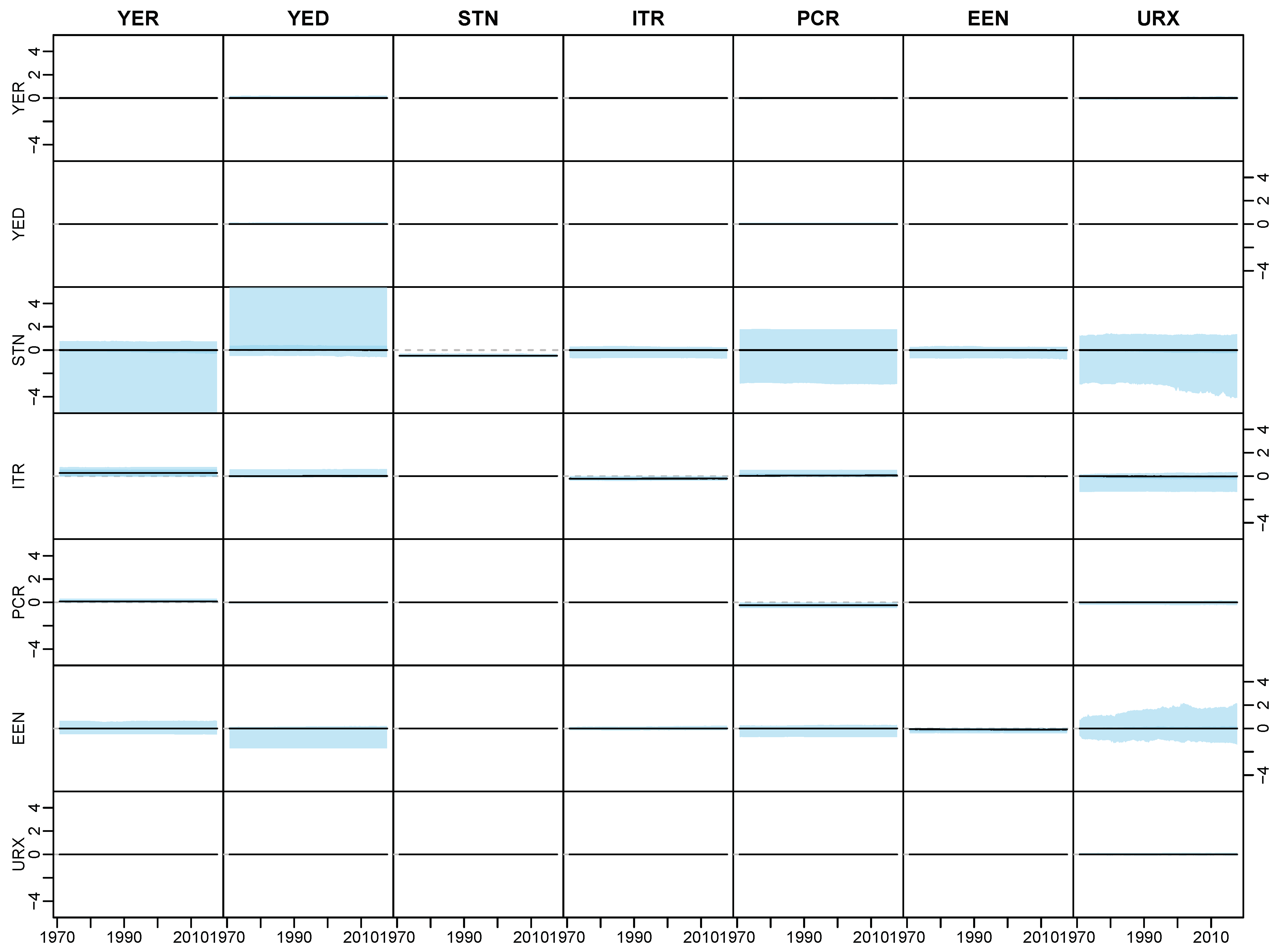
Appendix D.2. Posterior Paths

Figure A3. Each cell represents the corresponding state of the matrix Φ 1 , t , for t = 1 , , T , for the data described in Section 5.4. The solid line is the median and the shaded areas represent 50 % and 95 % posterior credible intervals under the triple gamma prior.
Econometrics 08 00020 g0a3
Figure A4. Each cell represents the corresponding state of the matrix Φ 2 , t , for t = 1 , , T , for the data described in Section 5.4. The solid line is the median and the shaded areas represent 50 % and 95 % posterior credible intervals under the triple gamma prior.
Econometrics 08 00020 g0a4

References

  1. Abramowitz, Milton, and Irene A. Stegun, eds. 1973. Handbook of Mathematical Functions. New York: Dover Publications. [Google Scholar]
  2. Armagan, Artin, David B. Dunson, and Merlise Clyde. 2011. Generalized beta mixtures of Gaussians. In Advances in Neural Information Processing Systems. Vancouver: NIPS, pp. 523–31. [Google Scholar]
  3. Belmonte, Miguel, Gary Koop, and Dimitris Korobolis. 2014. Hierarchical shrinkage in time-varying parameter models. Journal of Forecasting 33: 80–94. [Google Scholar] [CrossRef] [Green Version]
  4. Berger, James O. 1980. A robust generalized Bayes estimator and confidence region for a multivariate normal mean. The Annals of Statistics 8: 716–61. [Google Scholar] [CrossRef]
  5. Bhadra, Anindya, Jyotishka Datta, Nicholas G. Polson, and Brandon Willard. 2017a. The horseshoe+ estimator of ultra-sparse signals. Bayesian Analysis 12: 1105–31. [Google Scholar] [CrossRef]
  6. Bhadra, Anindya, Jyotishka Datta, Nicholas G. Polson, and Brandon Willard. 2017b. Horseshoe regularization for feature subset selection. arXiv arXiv:1702.07400. [Google Scholar] [CrossRef]
  7. Bhadra, Anindya, Jyotishka Datta, Nicholas G. Polson, and Brandon Willard. 2019. Lasso meets horseshoe: A survey. Statistical Science 34: 405–27. [Google Scholar] [CrossRef] [Green Version]
  8. Bitto, Angela, and Sylvia Frühwirth-Schnatter. 2019. Achieving shrinkage in a time-varying parameter model framework. Journal of Econometrics 210: 75–97. [Google Scholar] [CrossRef]
  9. Brown, Philip J., Marina Vannucci, and Tom Fearn. 2002. Bayes model averaging with selection of regressors. Journal of the Royal Statistical Society, Ser. B 64: 519–36. [Google Scholar] [CrossRef]
  10. Carriero, Andrea, Todd E. Clark, and Massimiliano Marcellino. 2019. Large Bayesian vector autoregressions with stochastic volatility and non-conjugate priors. Journal of Econometrics 212: 137–54. [Google Scholar] [CrossRef]
  11. Carvalho, Carlos M., Nicholas G. Polson, and James G. Scott. 2009. Handling sparsity via the horseshoe. Journal of Machine Learing Research W&CP 5: 73–80. [Google Scholar]
  12. Carvalho, Carlos M., Nicholas G. Polson, and James G. Scott. 2010. The horseshoe estimator for sparse signals. Biometrika 97: 465–80. [Google Scholar] [CrossRef] [Green Version]
  13. Chan, Joshua C. C., and Eric Eisenstat. 2016. Bayesian model comparison for time-varying parameter VARs with stochastic volatilty. Journal of Applied Econometrics 218: 1–24. [Google Scholar]
  14. Cottet, Remy, Robert J. Kohn, and David J. Nott. 2008. Variable selection and model averaging in semiparametric overdispersed generalized linear models. Journal of the American Statistical Association 103: 661–71. [Google Scholar] [CrossRef] [Green Version]
  15. Del Negro, Marco, and Giorgio E. Primiceri. 2015. Time Varying Structural Vector Autoregressions and Monetary Policy: A Corrigendum. The Review of Economic Studies 82: 1342–45. [Google Scholar] [CrossRef] [Green Version]
  16. Eisenstat, Eric, Joshua C.C. Chan, and Rodney W. Strachan. 2014. Stochastic model specification search for time-varying parameter VARs. SSRN Electronic Journal 01/2014. [Google Scholar] [CrossRef] [Green Version]
  17. Fagan, Gabriel, Jerome Henry, and Ricardo Mestre. 2005. An area-wide model for the euro area. Economic Modelling 22: 39–59. [Google Scholar] [CrossRef]
  18. Fahrmeir, Ludwig, Thomas Kneib, and Susanne Konrath. 2010. Bayesian regularisation in structured additive regression: A unifying perspective on shrinkage, smoothing and predictor selection. Statistics and Computing 20: 203–19. [Google Scholar] [CrossRef] [Green Version]
  19. Feldkircher, Martin, Florian Huber, and Gregor Kastner. 2017. Sophisticated and small versus simple and sizeable: When does it pay off to introduce drifting coefficients in Bayesian VARs. arXiv arXiv:1711.00564. [Google Scholar]
  20. Fernández, Carmen, Eduardo Ley, and Mark F. J. Steel. 2001. Benchmark priors for Bayesian model averaging. Journal of Econometrics 100: 381–427. [Google Scholar] [CrossRef] [Green Version]
  21. Figueiredo, Mario A. T. 2003. Adaptive sparseness for supervised learning. IEEE Transaction on Pattern Analysis and Machine Intelligence 25: 1150–59. [Google Scholar] [CrossRef] [Green Version]
  22. Frühwirth-Schnatter, Sylvia. 2004. Efficient Bayesian parameter estimation. In State Space and Unobserved Component Models: Theory and Applications. Edited by Andrew Harvey, Siem Jan Koopman and Neil Shephard. Cambridge: Cambridge University Press, pp. 123–51. [Google Scholar]
  23. Frühwirth-Schnatter, Sylvia, and Regina Tüchler. 2008. Bayesian parsimonious covariance estimation for hierarchical linear mixed models. Statistics and Computing 18: 1–13. [Google Scholar] [CrossRef] [Green Version]
  24. Frühwirth-Schnatter, Sylvia, and Helga Wagner. 2010. Stochastic model specification search for Gaussian and partially non-Gaussian state space models. Journal of Econometrics 154: 85–100. [Google Scholar] [CrossRef] [Green Version]
  25. Gelman, Andrew. 2006. Prior distributions for variance parameters in hierarchical models (Comment on Article by Browne and Draper). Bayesian Analysis 1: 515–34. [Google Scholar] [CrossRef]
  26. Griffin, Jim E., and Phil J. Brown. 2011. Bayesian hyper-lassos with non-convex penalization. Australian & New Zealand Journal of Statistics 53: 423–42. [Google Scholar]
  27. Griffin, Jim E., and Phil J. Brown. 2017. Hierarchical shrinkage priors for regression models. Bayesian Analysis 12: 135–59. [Google Scholar] [CrossRef]
  28. Jacquier, Eric, Nicholas G. Polson, and Peter E. Rossi. 1994. Bayesian analysis of stochastic volatility models. Journal of Business & Economic Statistics 12: 371–417. [Google Scholar]
  29. Johnstone, Iain M., and Bernard W. Silverman. 2004. Needles and straw in haystacks: Empirical Bayes estimates of possibly sparse sequences. The Annals of Statistics 32: 1594–649. [Google Scholar] [CrossRef] [Green Version]
  30. Kalli, Maria, and Jim E. Griffin. 2014. Time-varying sparsity in dynamic regression models. Journal of Econometrics 178: 779–93. [Google Scholar] [CrossRef] [Green Version]
  31. Kastner, Gregor. 2016. Dealing with stochastic volatility in time series using the R package stochvol. Journal of Statistical Software 69: 1–30. [Google Scholar] [CrossRef] [Green Version]
  32. Kastner, Gregor, and Sylvia Frühwirth-Schnatter. 2014. Ancillarity-sufficiency interweaving strategy (ASIS) for boosting MCMC estimation of stochastic volatility models. Computational Statistics and Data Analysis 76: 408–23. [Google Scholar] [CrossRef] [Green Version]
  33. Kleijn, Richard, and Herman K. van Dijk. 2006. Bayes model averaging of cyclical decompositions in economic time series. Journal of Applied Econometrics 21: 191–212. [Google Scholar] [CrossRef] [Green Version]
  34. Koop, Gary, and Dimitris Korobilis. 2013. Large time-varying parameter VARs. Journal of Econometrics 177: 185–98. [Google Scholar] [CrossRef] [Green Version]
  35. Koop, Gary, and Simon M. Potter. 2004. Forecasting in dynamic factor models using Bayesian model averaging. Econometrics Journal 7: 550–65. [Google Scholar] [CrossRef] [Green Version]
  36. Kowal, Daniel R., David S. Matteson, and David Ruppert. 2019. Dynamic shrinkage processes. Journal of the Royal Statistical Society, Ser. B 81: 673–806. [Google Scholar] [CrossRef] [Green Version]
  37. Ley, Eduardo, and Mark F. J. Steel. 2009. On the effect of prior assumptions in Bayesian model averaging with applications to growth regression. Journal of Applied Econometrics 24: 651–74. [Google Scholar] [CrossRef] [Green Version]
  38. Makalic, Enes, and Daniel F. Schmidt. 2016. A simple sampler for the horseshoe estimator. IEEE Signal Processing Letters 23: 179–82. [Google Scholar] [CrossRef] [Green Version]
  39. Nakajima, Jouchi. 2011. Time-varying parameter VAR model with stochastic volatility: An overview of methodology and empirical applications. Monetary and Economic Studies 29: 107–42. [Google Scholar]
  40. Park, Trevor, and George Casella. 2008. The Bayesian Lasso. Journal of the American Statistical Association 103: 681–86. [Google Scholar] [CrossRef]
  41. Pérez, Maria-Eglée, Luis Raúl Pericchi, and Isabel Cristina Ramírez. 2017. The scaled beta2 distribution as a robust prior for scales. Bayesian Analysis 12: 615–37. [Google Scholar] [CrossRef]
  42. Polson, Nicholas G., and James G. Scott. 2011. Shrink globally, act locally: Sparse Bayesian regularization and prediction. In Bayesian Statistics 9. Edited by José M. Bernardo, M. J. Bayarri, James O. Berger, Phil Dawid, David Heckerman, Adrian F. M. Smith and Mike West. Oxford: Oxford University Press, pp. 501–38. [Google Scholar]
  43. Polson, Nicholas G., and James G. Scott. 2012a. Local shrinkage rules, Lévy processes, and regularized regression. Journal of the Royal Statistical Society, Ser. B 74: 287–311. [Google Scholar] [CrossRef]
  44. Polson, Nicholas G., and James G. Scott. 2012b. On the half-Cauchy prior for a global scale parameter. Bayesian Analysis 7: 887–902. [Google Scholar] [CrossRef]
  45. Primiceri, Giorgio E. 2005. Time varying structural vector autoregressions and monetary policy. Review of Economic Studies 72: 821–52. [Google Scholar] [CrossRef]
  46. Raftery, Adrian E., David Madigan, and Jennifer A. Hoeting. 1997. Bayesian model averaging for linear regression models. Journal of the American Statistical Association 92: 179–91. [Google Scholar] [CrossRef]
  47. Ročková, Veronika, and Kenichiro McAlinn. 2020. Dynamic variable selection with spike-and-slab process priors. Bayesian Analysis. [Google Scholar]
  48. Sala-i-Martin, Xavier, Gernot Doppelhofer, and Ronald I. Miller. 2004. Determinants of long-term growth: A Bayesian averaging of classical estimates (BACE) approach. The American Economic Review 94: 813–35. [Google Scholar] [CrossRef] [Green Version]
  49. Scheipl, Fabian, and Thomas Kneib. 2009. Locally adaptive Bayesian p-splines with a normal-exponential-gamma prior. Computational Statistics and Data Analysis 53: 3533–52. [Google Scholar] [CrossRef] [Green Version]
  50. Strawderman, William E. 1971. Proper Bayes minimax estimators of the multivariate normal mean. The Annals of Statistics 42: 385–88. [Google Scholar] [CrossRef]
  51. Tibshirani, Ryan. 1996. Regression shrinkage and selection via the Lasso. Journal of the Royal Statistical Society, Ser. B 58: 267–88. [Google Scholar] [CrossRef]
  52. van der Pas, Stéphanie, Bas Kleijn, and Aad van der Vaart. 2014. The horseshoe estimator: Posterior concentration around nearly black vectors. Electronic Journal of Statistics 8: 2585–618. [Google Scholar] [CrossRef] [Green Version]
  53. Zhang, Yan, Brian J. Reich, and Howard D. Bondell. 2017. High dimensional linear regression via the R2-D2 shrinkage prior. Technical report. arXiv arXiv:1609.00046v2. [Google Scholar]
1
Let f θ j ( x ) and F θ j ( x ) be, respectively, the pdf and cdf of the random variable θ j . The cdf F θ j ( x ) of the random variable θ j is given by
F θ j ( x ) = Pr ( θ j x ) = Pr ( x θ j x ) = F θ j ( x ) F θ j ( x ) = 2 F θ j ( x ) ,
since f θ j ( x ) is symmetric around 0. The pdf f θ j ( x ) is obtained by taking the first derivative of F θ j ( x ) with respect to x:
f θ j ( x ) = d F θ j ( x ) d x = f θ j ( x ) / x .
2
Note that the X BP a , b -distribution has pdf
f ( x ) = 1 B ( a , b ) x a 1 ( 1 + x ) a + b .
Furthermore, Y = X / ( 1 + X ) follows the B a , b -distribution.
3
The pdf of a SBeta 2 a , c , ϕ -distribution reads:
f ( x ) = 1 ϕ a B ( a , c ) x a 1 ( 1 + x / ϕ ) ( a + c ) ,
4
Using (3), we obtain the following prior for ρ j = 1 / ( 1 + ψ j 2 ) by the law of transformation of densities:
p ( ρ j ) = 1 Γ ( a ξ ) a ξ κ B 2 2 a ξ ( 1 ρ j ) a ξ 1 ρ j ( a ξ + 1 ) exp 1 ρ j ρ j a ξ κ B 2 2 .
5
The pdf of the GIG p , a , b -distribution is given by
f ( x ) = ( a / b ) p / 2 2 K p ( a b ) x p 1 e 1 2 ( a x + b / x ) ,
where K p ( z ) is the modified Bessel function.
Figure 1. Marginal prior distribution of θ j under the triple gamma prior with a ξ = c ξ = 0.1 with κ B 2 = 2 , in comparison to the Horseshoe prior with ϕ ξ = 1 , the double gamma prior with a ξ = 0.1 and κ B 2 = 2 and the Lasso prior with κ B 2 = 2 . Spike (left-hand side) and tail (right-hand side) of the marginal prior.
Econometrics 08 00020 g001
Figure 2. Marginal univariate shrinkage profile under the triple gamma prior with a ξ = c ξ = 0.1 , in comparison to the Horseshoe prior, the double gamma prior with a ξ = 0.1 and the Lasso prior. κ B 2 = 2 for all the prior specifications.
Econometrics 08 00020 g002
Figure 3. “Prior density” of shrinkage profiles for (from left to right) a Lasso prior, a double gamma prior with a ξ = 0.2 , a Horseshoe prior and a triple gamma prior with a ξ = c ξ = 0.1 , when κ B 2 is random. The solid line is the median, while the shaded areas represent 50% and 95 % prior credible bands. We have used κ B 2 G 0.01 , 0.01 for the Lasso and the double gamma, 2 / κ B 2 F 1 , 1 for the Horseshoe and 2 / κ B 2 F 0.2 , 0.2 for the triple gamma.
Econometrics 08 00020 g003
Figure 4. Bivariate shrinkage profile p ( ρ 1 , ρ 2 ) for (from left to right) the Lasso prior, the double gamma prior with a ξ = 0.1 , the Horseshoe prior, and the triple gamma prior with a ξ = c ξ = 0.1 , with κ B 2 = 2 for all the priors. The contour plots of the bivariate shrinkage profile are shown, together with 500 samples from the bivariate prior distribution of the shrinkage parameters.
Econometrics 08 00020 g004
Figure 5. Posterior path against time for a constant non-significant parameter β j , t i in the sparse regime.
Econometrics 08 00020 g005
Figure 6. Posterior inclusion probability for the θ i j β ’s in the sparse and dense regime, under the triple gamma prior, the Horseshoe prior, the Lasso prior and the double gamma prior. The true values of the θ i j β ’s are reported in each cell.
Econometrics 08 00020 g006
Figure 7. Posterior inclusion probability for state parameters β i j β associated with the first lag (on the left) and with the second lag (on the right), for the Euro Area data under the triple gamma prior, the Horseshoe prior, the double gamma prior and the Lasso prior.
Econometrics 08 00020 g007
Figure 8. Posterior inclusion probability for θ i j β ’s associated with the first lag on the left and with the second lag on the right, for the Euro Area data under the triple gamma prior, the Horseshoe prior, the double gamma prior and the Lasso prior.
Econometrics 08 00020 g008
Figure 9. Posterior median of β i j β under the triple gamma, Horseshoe, double gamma and Lasso for the Euro area model. The vertical lines delimit the intercept, first and second lag, respectively.
Econometrics 08 00020 g009
Figure 10. Posterior median of θ i j β under the triple gamma, Horseshoe, double gamma and Lasso for the Euro area model. The vertical lines delimit the intercept, first and second lag, respectively.
Econometrics 08 00020 g010
Table 1. Priors on θ j which are equivalent to (top) or special cases of (bottom) the triple gamma prior.
Prior for θ j a ξ c ξ κ B 2 ϕ ξ
N 0 , ψ j 2 , ψ j 2 G G a ξ , c ξ , ϕ ξ normal-gamma-gamma a ξ c ξ 2 c ξ ϕ ξ a ξ ϕ ξ
N 0 , 1 κ j 1 , κ j TPB a ξ , c ξ , ϕ ξ generalized beta mixture a ξ c ξ 2 c ξ ϕ ξ a ξ ϕ ξ
N 0 , ψ j 2 , ψ j 2 SBeta 2 a ξ , c ξ , ϕ ξ hierarchical scaled beta2 a ξ c ξ 2 c ξ ϕ ξ a ξ ϕ ξ
DE 0 , 2 ψ j , ψ j 2 G c ξ , 1 λ 2 normal-exponential-gamma1 c ξ 2 λ 2 c ξ 1 λ 2
N 0 , τ 2 ψ j 2 , ψ j t 1 Horseshoe 1 2 1 2 2 τ 2 τ 2
N 0 , 1 κ j 1 , κ j B 1 / 2 , 1 Strawderman-Berger 1 2 141
N 0 , τ 2 ξ ˜ j , ξ ˜ j G a ξ , a ξ double gamma a ξ 2 τ 2 -
N 0 , τ 2 ξ ˜ j , ξ ˜ j E 1 Lasso1 2 τ 2 -
t ν 0 , τ 2 half-t ν 2 2 τ 2 -
t 1 0 , τ 2 half-Cauchy 1 2 2 τ 2 -
N 0 , B 0 normal 2 B 0 -

