BACE and BMA Variable Selection and Forecasting for UK Money Demand and Inflation with Gretl


1
Faculty of Finance and Management, WSB University in Torun, ul. Młodzieżowa 31a, 87-100 Toruń, Poland
2
Faculty of Economic Sciences and Management, Nicolaus Copernicus University, ul. Gagarina 13a, 87-100 Toruń, Poland
*
Author to whom correspondence should be addressed.
Econometrics 2020, 8(2), 21; https://0-doi-org.brum.beds.ac.uk/10.3390/econometrics8020021
Submission received: 27 September 2019
/
Revised: 27 April 2020
/
Accepted: 20 May 2020
/
Published: 22 May 2020
(This article belongs to the Special Issue Bayesian and Frequentist Model Averaging)
Abstract
:In this paper, we apply Bayesian averaging of classical estimates (BACE) and Bayesian model averaging (BMA) as an automatic modeling procedures for two well-known macroeconometric models: UK demand for narrow money and long-term inflation. Empirical results verify the correctness of BACE and BMA selection and exhibit similar or better forecasting performance compared with a non-pooling approach. As a benchmark, we use Autometrics—an algorithm for automatic model selection. Our study is implemented in the easy-to-use gretl packages, which support parallel processing, automates numerical calculations, and allows for efficient computations.
JEL Classification:
C22; C52; C531. Introduction
In this paper we consider two procedures of variable selection and forecasting for linear dynamic single-equation models: Bayesian averaging of classical estimates (BACE), introduced by Sala-i-Martin et al. (2004) and Bayesian model averaging (BMA) (see Raftery et al. 1997). The BACE and BMA methods are natural extension of the standard Bayesian inference methods in which one does not only make inference using single model, but also allowing pooling approach with combined estimation and prediction. As a benchmark we use Autometrics procedure which is non-pooling method based on general-to-specific approach with multiple path of searching algorithm implemented in OxMetrics software (see Doornik 2009; Doornik and Hendry 2013). We present empirical results for two non-trivial UK macroeconometric models: demand for narrow money (see Krolzig and Hendry 2001), and long-term inflation (see Hendry 2001).
In the last two decades we can observe a growing number of publications related to Bayesian model averaging in many fields of science like engineering, medicine, biology, sociology and others (see Fragoso et al. 2018). Not surprisingly, this type of approach has also been long-used in economics and it is still important, especially for identification of the sources of economic growth (Fernández et al. 2001a, 2001b; Błazejowski et al. 2019). The ideas stated in this paper were reviewed, among others, by Hoeting et al. (1999) and Wasserman (2000). A comprehensive study on the use of model averaging in economics, both from the frequentist and Bayesian approaches, was discussed in Steel (2019).
The BACE approach is an approximation of BMA and it is not purely Bayesian but relies on Schwarz approximation to compute the Bayes factor (see Ley and Steel 2009). Nevertheless, both the BACE and BMA approaches account for model uncertainty, which often requires the consideration of many possible linear combinations of variables and lead to a large model space that needs to be explored and then demands intensive computational effort. As an approximation, BACE is usually faster than the standard BMA approach; nevertheless, obtaining the output in a reasonable amount of time still remains a significant challenge, especially in time-series modeling and forecasting. Raftery et al. (1997) showed that standard variable selection procedures lead to different estimates and conflicting conclusions about the main questions of interest. Moreover, econometric models that are firmly based on economic theory do not always work for forecasting. The BACE and BMA approaches combine the knowledge obtained from many possible models and accounts for uncertainty by averaging the parameter estimates from different specifications. Consequently, both methods can better identify significant determinants of a dependent variable and generate more accurate forecasts without any specific knowledge.
In BACE and BMA we can penalize large dynamic models using different model prior assumptions putting higher probabilities for more parsimonious models. This type of approach does not cover all possible solutions. One of the potential alternative is assigning lower prior probabilities over lags length, such as Minnesota Prior (see Doan et al. 1984). We also assume stability of the relation between dependent and independent variables over time and, as a consequence, all slope parameters and other posterior characteristics in our BACE and BMA packages are time invariant. In the case of time-varying parameters, it is possible to employ dynamic model averaging presented in Drachal (2018); Raftery et al. (2010).
The remainder of this paper is structured as follows. In Section 2, we discuss some aspects of BACE. Section 3 briefly outlines Bayesian model averaging for dynamic linear regression models along with short information about implementation of both packages in the gretl. In Section 4 we provide basic information about Autometrics—a PcGive module for automatic model selection. Section 5 presents empirical results for two selected UK macroeconometric models: demand for narrow money and long-term inflation. In this section, we also compare the variable selection strategies and forecasting performance of BACE and BMA with those of Autometrics. Additionally, in Section 6 we analyze the robustness and computational run-times of BACE and BMA. Finally, we conclude the paper in Section 7.
2. The BACE Method
In Sala-i-Martin et al. (2004), the authors proposed averaging parameter estimates using a technique—Bayesian averaging of classical estimates—that enabled the measurement of the importance of particular potential regressors. In this method, parameter estimates are obtained by applying ordinary least squares (OLS) and then averaged across all possible combinations of models. The BACE approach is not purely Bayesian but relies on Schwarz approximation to compute the Bayes factor. This approach is an alternative to the familiar and earlier-applied BMA technique, from which it differs i.e., by using non-informative prior assumptions of regression parameters1. A full discussion that compares BACE and BMA is presented in Ley and Steel (2009).
Among the many articles that have applied the BACE technique are van Dijk (2004) for US inflation and Białowolski et al. (2014) for gross domestic product, inflation, and unemployment in Poland. Jones and Schneider (2006) used BACE analysis to verify the human capital effect on economic growth, while Mapa and Briones (2007) and Simo-Kengne (2016) used BACE analysis to obtain variables associated with economic growth. Cuaresma and Doppelhofer (2007) extended the BACE approach by allowing for the uncertainty of nonlinear threshold effects to identify determinants of long-term economic growth. Bergh and Karlsson (2010) applied BACE to investigate the relation between government size and the control of economic freedom and globalization for a panel of rich countries. In an empirical investigation of industrial production forecasting, Feldkircher (2012) focused on the forecasting performance resulting from model averaging by measuring the root-mean-square error (RMSE). Albis and Mapa (2014) used BACE to verify misspecification issues in vector autoregressive models for artificial data.
Let us consider the following dynamic linear regression model :
where y is a vector of observations, is a matrix, where and is a matrix containing lagged values of dependent variable, while is matrix of exogenous variables, is a vector of unknown parameters, where , , is an vector of errors that are assumed to be normally distributed (i.e., ) and denotes a normal distribution with location and covariance .
From OLS estimates (see Sala-i-Martin et al. 2004), we can calculate the approximation of the posterior probability of model (i.e., ) using the following formula:
where and are the OLS sum of squared errors, denotes the total number of potential combinations of K independent variables, and and are the number of regression parameters and . In , denotes the density of the marginal distribution of y conditional on model .
Prior probabilities and of models and are binomially distributed; that is,
The binomial distribution implies that we only need to specify a prior expected model size , where . For example, if we define the value of , then our BACE package will automatically produce a value of prior inclusion probability for all competitive models. If , then the prior expected model size is equal to the average of the number of potential regressors, and the model prior distribution is uniform and reflects a lack of previous knowledge about the models.
Using BACE, we can also easily evaluate the mean and variance of the posterior distribution of regression parameters for the whole model space (see Leamer 1978; Sala-i-Martin et al. 2004):
where and are the OLS estimates of from model .
Another useful and popular characteristic of the BACE approach is posterior inclusion probability (PIP), which is defined as the posterior probability that the variable is relevant in the explanation of the dependent variable (see Leamer 1978; Mitchell and Beauchamp 1988). In our case, the PIP is calculated as the sum of the posterior model probabilities for all of the models that include a specific variable:
For model averaging, a Bayesian pooling strategy can also provide useful information about future observations of the dependent variable on the basis of the whole model space:
where and denote the mean and variance of future observations .
3. The BMA Method
Another model building strategy is Bayesian model averaging wherein we can make an inference based on full posterior distribution. From Bayesian perspective uncertainty is a natural way of decision making process and therefore it can be easily included in the model selection rules (Koop 2003; Zellner 1971). Among the many seminal papers about Bayesian model averaging are Hoeting et al. (1999) and Fernández et al. (2001a, 2001b). The most recent detailed overview is presented in Steel (2019).
Once again, we are dealing with a problem which model and variables are the most appropriate in the analysis of the dependencies, but in this case we use a natural and explicit way of combining prior information with data, without any approximation of marginal data density and Bayes factors. We consider two variants of BMA framework. The first one where we impose stationary conditions for autoregressive parameters, and the second one without restrictions.
Now let us consider the first one:
where y is a vector of T observations, is matrix, and is a vector of parameters, is a vector of dimensions with a normal distribution , where is a variance of random error and is an identity matrix of size T. Moreover , where is a matrix containing lagged values of dependent variable, while is matrix of exogenous variables. Furthermore, is a vector of unknown parameters, where , , and is stationary region for the parameters of autoregressive processes. We also assume that we observe initial values .
Let us consider a prior density of the following form:
where:
and denotes the multivariate normal density with mean and covariance matrix , is the indicator function, is -vector of prior means for regression coefficients and is a positive definite prior covariance matrix of the form:
For the error precision h which is defined as we use noninformative prior:
The factor of proportionality is part of the so-called g-prior, as introduced in Zellner (1986). In our research we use Benchmark prior, recommended by Fernández et al. (2001a):
Assuming the prior structure in Equation (10) we obtain the following joint posterior density:
where is normalizing constant and is normal-gamma density (see Koop et al. 2007). In our case constant plays important role to obtain the Bayes factor between competitive models and can be obtained by Monte Carlo simulations.
Using the properties of normal-gamma density, Equation (15) leads to:
where
and . We also have:
where .
The marginal data density as well as posterior means and standard deviations of regression coefficients can be calculated numerically using Monte Carlo integration by sampling from the posterior distribution in Equation (15). In our case, we first draw error precision h from Equation (17) and then we draw from Equation (16). We only accept those candidate values which lie in stationary region for the parameters of autoregressive processes. The constant can be calculated as an inverse of the acceptance ratio i.e., inverse of the fraction of random numbers accepted in Monte Carlo simulation.
The posterior probability of any variant of regression model can be calculated by the following formula, which is crucial for Bayesian model averaging:
where denote the prior probabilities of competitive models (see Equation (3)). Other characteristics, like posterior model probabilities (PIP) as well as the mean and variance of the posterior distribution of regression parameters for the whole model space can be calculated in the same manner as described for BACE method.
In case of BMA variant without stationary restrictions for the parameters of autoregressive processes, we assume that and Equations (11), (15) and (16) takes the following form, while the other equations remain unchanged:
BACE and BMA in Gretl
In order to perform Bayesian averaging of classical estimates, we used the BACE 2.0 package2. This code implements an automatic BACE procedure that is available in the gretl3 program as an open-source software. In the procedure’s main window, we can specify e.g., the following parameters: the list of independent variables, the prior distribution over the model space, the number of out-of-sample forecasts, and general parameters for the Monte Carlo simulation. As a result, the BACE package prints basic posterior characteristics, such as PIP, and the posterior means of coefficients, together with their standard errors. In addition, the package presents rankings of the most probable specifications according to their explanatory power and generates forecasts of the dependent variable.
In this paper we also use a software package that implements Bayesian model averaging for Autoregressive Distributed Lag models BMA_ADL ver. 0.9 in gretl4. The BMA_ADL package as well as the output is similar to BACE package. Although these two packages are similar there is a principle difference between them. In BMA_ADL we draw samples from posterior distribution of slope parameters and we check roots of characteristic polynomial of the autoregressive process, although this feature can be explicitly switched off by user. Detailed information about the package can be found in Błażejowski and Kwiatkowski (2020).
Since exploration of many possible models demands intensive computational effort, we run BACE and BMA_ADL through the Message Passing Interface (MPI)5. It is especially useful for a large number of explanatory variables, which results in a computational complexity that exceeds the computing power of modern PCs, because it performs parallel computations through MPI.
Both packages are written in gretl’s internal scripting language Hansl (see Cottrell and Lucchetti 2019b) with an easy-to-use graphical user interface (GUI). Therefore, they can be treated as an automatic model selection procedure and would be a useful for users who are not familiar with model averaging.
4. Autometrics
Autometrics procedure of variables model selection is built on the basis of PcGets module implemented in OxMetrics software and is is fully described in Doornik (2009) and Doornik and Hendry (2013). This conception is based on general-to-specific approach with multiple path of searching (reducing) algorithm. The assumption underlying empirical model selection is discovering the local data generating process (LDGP), which is tend to explain the relations which occur in real world in the space of available variables. One needs to select the model from the set of potential specifications ensuring that model is congruent and encompasses LDGP. The crucial issue here is test-based reduction strategy (see Desboulets 2018).
The procedure of selecting variables in Autometrics is proceed in following stages. The starting point for automatic procedure is general unrestricted model (GUM), which should remain congruent and include all potentially relevant variables according to sample size, theoretical, or empirical considerations. This solution increases chance that LDGP is nested in GUM and can be discovered. The variables, which have strong importance and influence should remain in model and the less significant ones should not be retained. The mis-specification test is applied to ensure the congruence postulate and to avoid badly-specified GUM. Additionally, encompassing test is used to evaluate if small model can explain larger one, which is encompassed within. Such a procedure can be treated as progressive research strategy of reduction and defines partial order of considered model specifications (see Hendry et al. 2008).
Autometrics ensures the tree-search approach for examining the whole model space using three strategies of path evaluation: pruning, bunching and chopping (see Hendry and Doornik 2014). Before the main multi-path reduction of variables is launched, the pre-search is initiated to eliminate most insignificant and irrelevant variables. During reductions and simplifications diagnostic tests are employed to ensure the congruence and to find valid specification. The terminal model is received at the end of each branch of the tree-search algorithm. Moreover, Autometrics also take into consideration following modeling issues: cointegration, functional form, economic theory or data accuracy.
Application of Autometrics or PcGets can be found in works, for example: Clements and Hendry (2008); Hendry (2001) for UK inflation, Hendry (2011) for consumers’ expenditures, Castle et al. (2012) for US real interest rates, Ericsson and Kamin (2009) for Argentine broad money demand, Marczak and Proietti (2016) for industrial production, Kamarudin and Ismail (2016) for water quality index, or Ackah and Asomani (2015) for renewable energy.
5. Empirical Results
In this section, we analyze the BACE and BMA results for data used in two well-known dynamic macroeconometric models: model for M1 money demand in UK (UKM1), which was proposed in Hendry and Ericsson (1991), and the long-term UK inflation model, as introduced in Hendry (2001). We focus on the modeling and forecasting of narrow money and inflation in the UK using the BACE and BMA methods along with the Autometrics program6. We analyze the estimation results using standard posterior characteristics, such as posterior inclusion probabilities, the posterior means of regression parameters, and the posterior standard deviations, as defined in Section 2. We compare forecasting accuracies using three measures, namely, root-mean-square error (RMSE), mean average percentage error (MAPE), and Theil’s U coefficient (see Theil 1966, pp. 33–36) divided into three factors: bias proportion UM (measures differences between averages of actual and predicted values), regression proportion UR (evaluates the slope coefficient from a regression of changes in actual values on changes in predicted values), and disturbance proportion UD (measures proportion of forecast error associated with random disturbance). Two first factors stand for systematic error and should be 0, while disturbance proportion is an unsystematic element and should equal 1.
Based on the methods discussed here, we also consider two additional models associated with BACE and BMA output. Barbieri and Berger (2004) introduced median probability model, which is defined as the model consisting of those variables which have an overall posterior probability greater than or equal to 0.5 of being in a model. According to the authors, median probability model considerably outperforms the most probable model in terms of predictive accuracy. Therefore it seems reasonable to include this model in our analysis and compare its forecasting performance.
5.1. Modeling and Forecasting Demand for Narrow Money in the UK: UKM1
We based the first empirical illustration on the UKM1 model proposed in Hendry and Ericsson (1991) in the following form:
where small letters indicate the log-transformed variables defined as follows7:
- : nominal narrow money, M1 aggregate in million £,
- : real total final expenditure (TFE) for 1985 prices in million £,
- : deflator of TFE,
- : net interest rate of the cost of holding money (calculated as the difference between the three-month interest rate and learning-adjusted own interest rate).
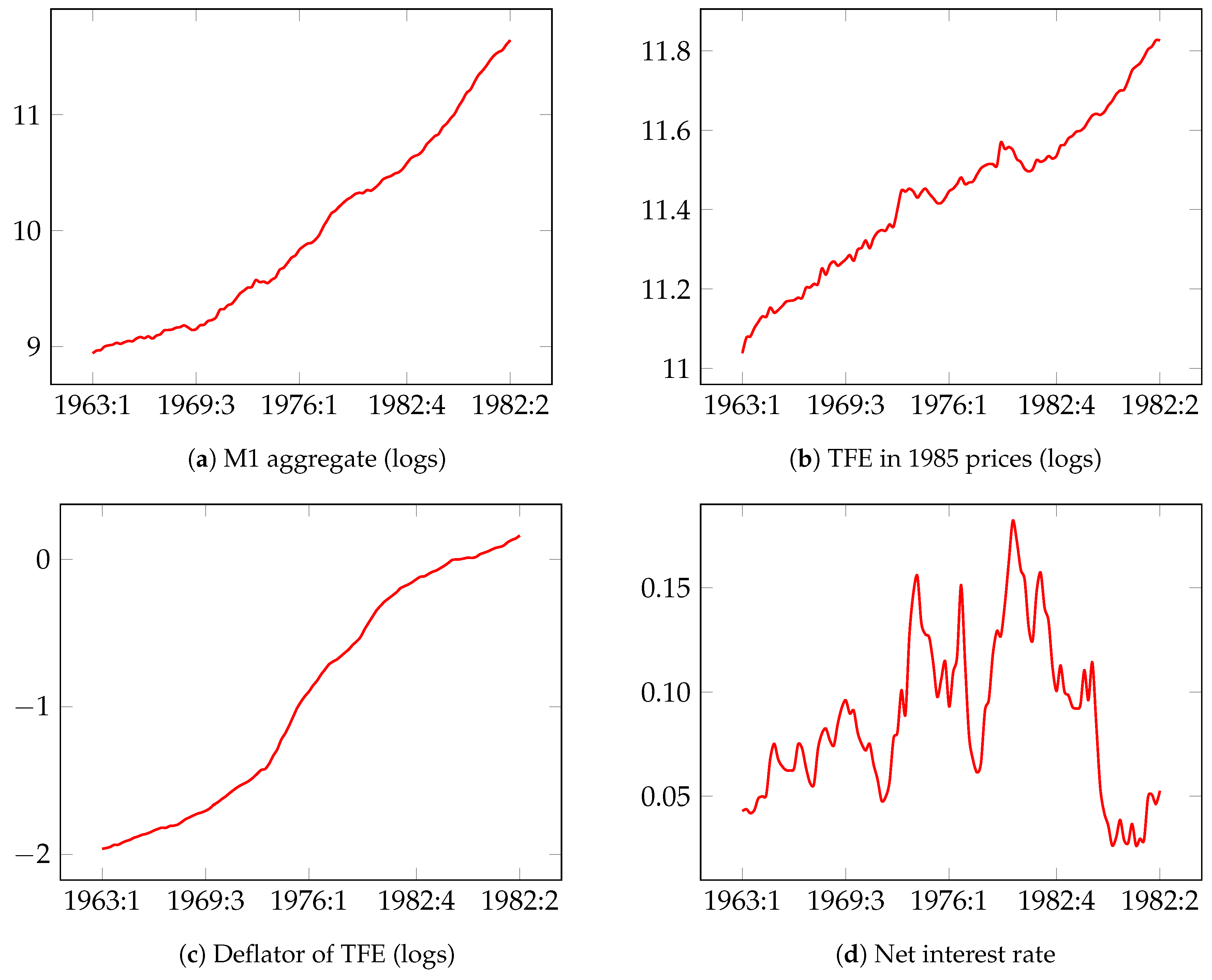
The data for the UK narrow money M1 aggregate are quarterly and span from 1964:3 to 1989:28. Figure 1 presents plots of the time series used in the analysis.
Model (27) was later replicated as an unrestricted autoregressive distributed lag (ADL) model in PcGets (see Krolzig and Hendry 2001, p. 29). In their paper, narrow money was measured in nominal terms instead of real terms, so the ADL representation of the general unrestricted model (GUM) was defined as follows:
After reduction9, they obtained the following empirical model:
In our research, following Krolzig and Hendry (2001), we estimated the GUM in the form shown in Equation (28) using the sample 1964:1–1985:2 and used the last 4 years (1985:3–1989:2) for forecasting purposes. We compared the variable selection and forecasting accuracy of BACE and BMA with those of Autometrics, which is an alternative automatic model selection procedure. Table 1 presents the estimation and variable selection results for UKM1 in the ADL form, Equation (28). Model space consists of = 1,048,576 specifications that must be considered. The total number of variables is 20, including current values of an explanatory variables and their lags (up to order 4), lagged values of the dependent variable (up to order 4) and constant.
According to the results in Table 1, the variables used in the BACE analysis can be divided into three groups: high-probability determinants with , medium-probability determinants with , and low-probability determinants (the remaining variables) with . The top four most probable variables are the same as those selected by Autometrics, although only three of them are classified as highly probable determinants (one variable, i.e., is close to being highly probable). This discrepancy between the two selections can be explained by the fact that the Autometrics model, which is the most probable one in BACE, has only 1.53% of the total posterior probability mass (see Table 2).
In case of BMA with stationarity restrictions, we get similar results although there are some slight changes. Again the top four most probable variables are the same as those selected by BACE and Autometrics, however the only two them can be classified as highly probable, while in the group of medium-probability determinants we can include: . The most likely model is again the model selected by Autometrics, although in this case the posterior probability for the top model is higher than in BACE and equals to 8.09% (see Table 3). The BMA procedure without stationarity restrictions points the and as highly probable variables, while and are medium probable. The most probable model is still the same as indicated in BMA with stationarity restrictions, but models and have changed the order in the list (see Table 4). In the vast majority of cases, BMA PIP coefficients take lower values than in the case of BACE. As a consequence, we find little difference in posterior mean and variance of regression parameters comparing BACE to BMA. Nevertheless, it is difficult to state clearly which point estimates are closer to the results obtained by Autometrics, however, the BACE ranking is more consistent with the Autometrics output. It seems that the both BMA methods prefer a more parsimonious specifications that do not include some variables found to be important in the BACE and Autometrics.
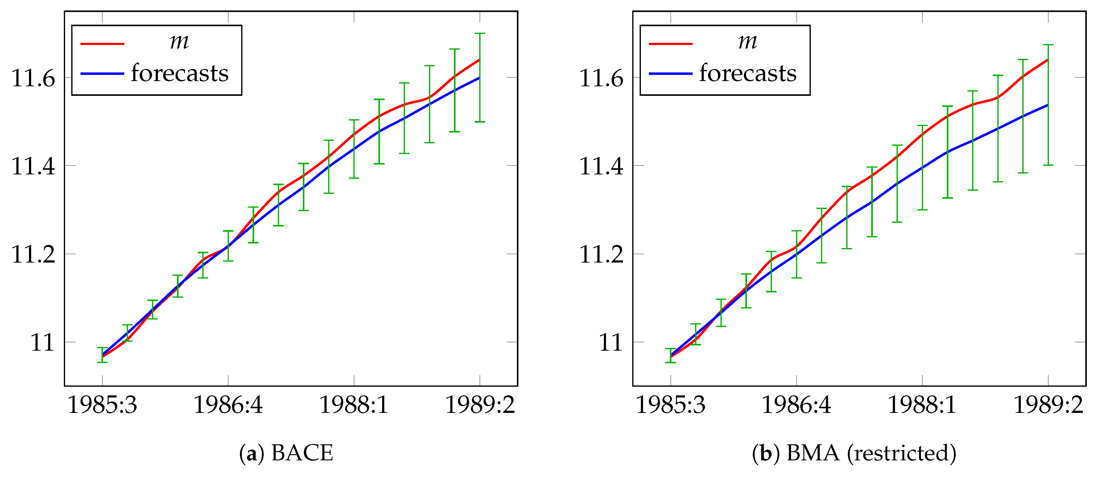
In the next step, we decided to compare the accuracy of forecasts. Table 5 presents the BACE, B A (with and without stationarity restriction) and Autometrics forecasts of nominal narrow money in the UK for the period from 1985:3 to 1989:2, which covers 16 quarters. The second column includes the logs of the actual values of the dependent variable. The next columns contain the weighted averages of individual model forecasts and errors for BACE, BMA, and Autometrics, respectively. Additionally, we include results for so-called median probability models introduced by Barbieri and Berger (2004). Moreover, the five bottom rows of the table contain well-known measures of forecast error: RMSE, MAPE, and Theil’s U coefficients.
Two accuracy measures indicate that the BACE forecasts are relatively close to the real values of nominal narrow money in the UK. For BACE, RMSE is 0.0224 and MAPE is 0.17%, while RMSE and MAPE for BMA with stationarity restrictions are 0.0592 and 0.43%, respectively. Forecast generated by BMA without stationarity restrictions have slightly lower forecast errors then forecasts from BMA with stationarity restrictions. In the other cases, i.e., for Autometrics and median probability models the results are in the range of 0.0994–0.1018 and 0.72–0.74%, respectively, while both median BMA approaches give exact equal results. It means that the RMSE calculated for BACE is two and a half times smaller than the RMSE resulting from BMA and almost five times smaller than for Autometrics. We can see almost the same scenario for MAPE measure where BACE measure returns the smallest errors. As the last conclusion about these results is that the median probability models do not outperform the mixture of models in terms of predictive performance.
For all methods, the largest factor of forecast error is bias proportion, which has a considerable impact on forecast accuracy, although for BACE is the smallest one. This is clearly reflected in Figure 2, which shows the actual and forecasted values of nominal narrow money. In this figure, the bias in the forecasts generated by BMA, Autometrics and two other methods substantially grows as the forecast horizon increases.
One potential explanation of this observation is that the forecasts in Autometrics and median probability models are generated by only one model. According to the BACE and BMA with stationarity restrictions results, the use of a single model leaves 98.5% and 91.9% of the total posterior probability mass. On the other hand, BACE and BMA calculates forecasts from the whole model space and accounts for the mixture of all considered specifications, which are weighted by their posterior probabilities.
5.2. Modeling and Forecasting Long-Term UK Inflation
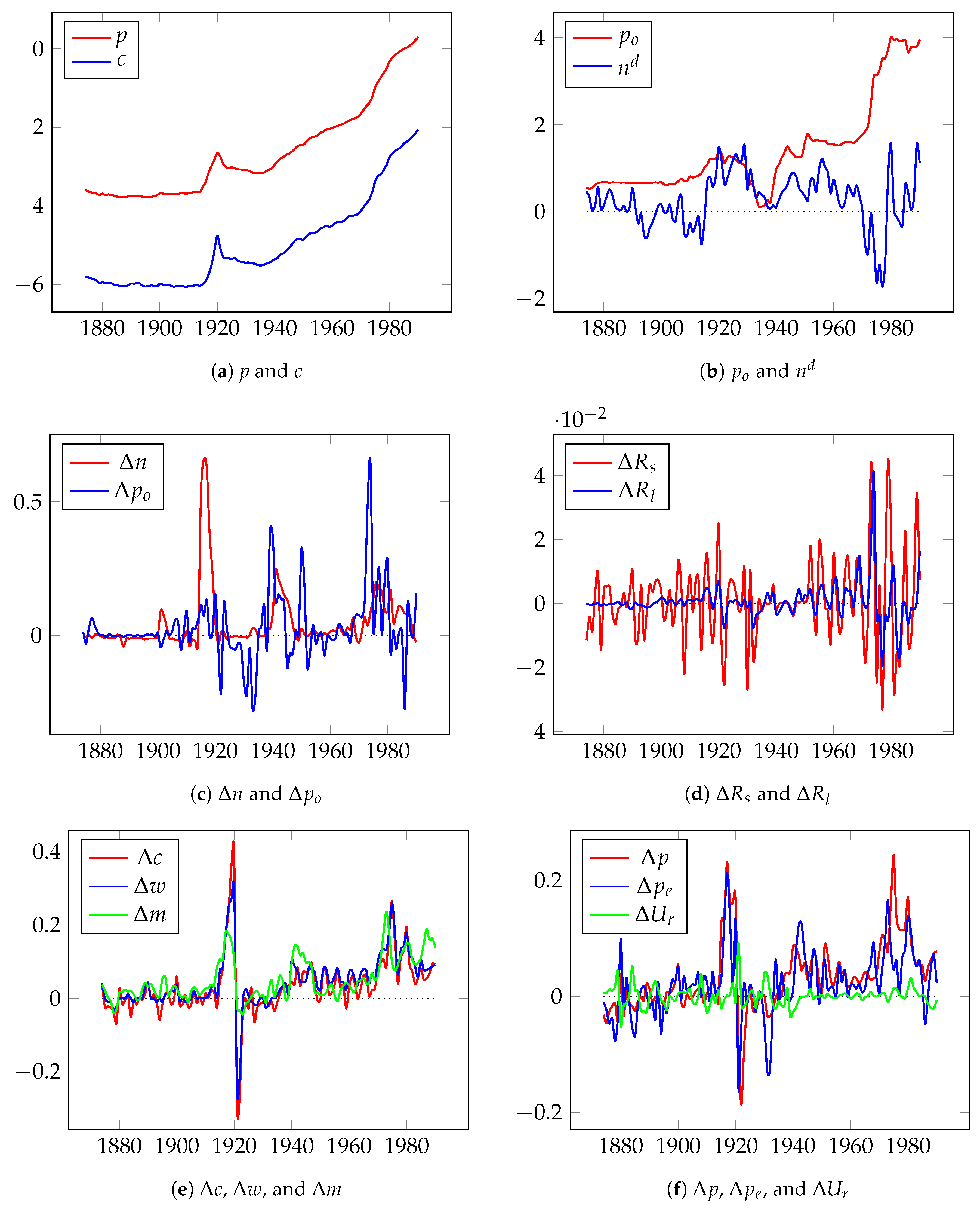
In the second empirical example, we used the long-term UK inflation model developed in Hendry (2001) for 1875–1991 years . The data set10 used in this research is described in Table 6, and Figure 3 presents the time-series plots (small letters indicate log-transformed variables).
The final specification after a number of variable transformations and model pre-reduction was as follows11) (see Hendry 2001):
where , , and is a combination of year indicator dummies. Model space consists of = 1,048,576 linear combinations that must be considered. After the reduction at a 1% significance level, specification in Equation (30) was reduced to the following empirical model (see Hendry 2001):
The results in Table 7 show that the BACE, BMA, and Autometrics identify the same set of significant determinants of UK inflation as in Hendry (2001). Moreover, both BMA procedures, with and without stationarity restrictions, give exactly the same results. This can be explained by the fact that dependent variable is far away from non-stationary region, so imposing stationarity restrictions does not result in rejecting any of draws from posterior. Hereafter, we formulate comments without division into restricted or unrestricted case. BACE and BMA indicate that the following variables are highly probable: . Autometrics selects the same set, reducing model (30) at the 1% significance level.
Table 8, Table 9 and Table 10 present the BACE and BMA posterior probability and coefficient estimates for the top 10 models. In the case of BACE the most probable model has a posterior probability of 21.9%, while the second model in the ranking has a probability of 6.4%. For the other models, the posterior probability does not exceed 4.7%. Although the posterior probability of the highest-ranked model is more than three times larger than that of the second model , an inference that is based only on leaves 78.1% of the posterior probability mass. As a consequence, estimates of the average mean of coefficients are slightly different from those in Autometrics. We can meet a similar situation in the case of BMA, although the highest-ranked model is even more preferred by the data with posterior probability equals to 32.66%. The second model in the ranking is almost two times less likely.
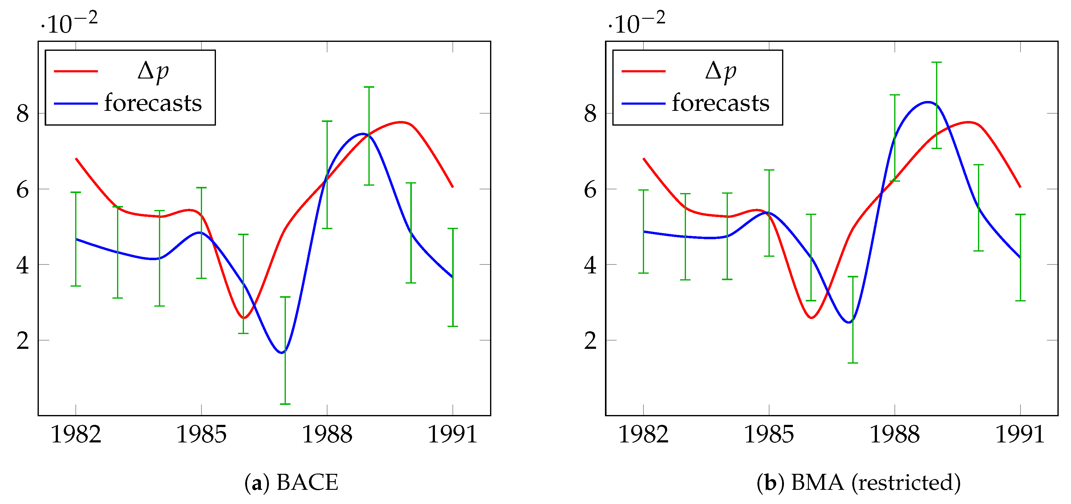
Table 11 presents detailed information about the predictions for UK inflation resulting from BACE, BMA, Autometrics, and median probability models. This table includes actual values, forecast values, and forecast standard errors, as well as accuracy measures, for the period from 1982 to 1991, which covers 10 years. The actual and forecast values of UK inflation are presented in Figure 4. For BACE, RMSE is 0.0179 and MAPE is 26.06%, for BMA we have RMSE—0.0175 and MAPE—25.85%, while RMSE and MAPE in Autometrics are 0.0151 and 25.06%, respectively. Forecast errors of the median probability models are the largest compared to other methods. As we can see BACE, BMA, and Autometrics generate forecasts of almost the same quality, but the sources of errors are different. For BACE and BMA, the greatest factor of forecast error is bias proportion, while the greatest factor for Autometrics is disturbance proportion.
One explanation of the equivalent forecasting performances is the fact that, according to the results in Table 8, Table 9 and Table 10, the top 10 most probable specifications have almost the same set of nine the most probable variables and cover over 50% of the posterior probability mass, including the second-ranked model () selected by Autometrics.
6. Robustness and Run Time Analysis
6.1. Robustness
In order to confirm the empirical findings for variable and model selection obtained by BACE and BMA, we performed a robustness analysis using different prior model assumptions. We apply philosophy proposed in Osiewalski and Steel (1993) and we set different variants of the prior average model size in order to penalize large models. In Section 5, the prior average model size is set to (where K is the total number of independent variables). This means that we do not prefer any specification, so all possible models are equally probable. We considered robustness scenario as different specifications of prior model size, estimating the models in Equations (28) and (30) using three competitive variants: , , and (the most restrictive case). Table 12 and Table 13 present the BACE estimates, Table 14 and Table 15 show results for BMA with stationarity restrictions, while Table 16 and Table 17 relate to results for BMA without stationarity restrictions.
According to the results concerning BACE method, which are presented in Table 12 and Table 13, there are no substantial differences in the output between , , and . Similar conclusion can be formulated for BMA outcome included in Table 14, Table 15, Table 16 and Table 17. Moreover, comparing the results in Table 12, Table 13, Table 14, Table 15, Table 16 and Table 17 with those in Table 1 and Table 7 reveals that the observed differences are negligible.
6.2. BACE and BMA Run Times
Table 18, Table 19 and Table 20 present computational timings12 of BACE and BMA analysis conducted in two general variants, with and without forecasting, for two earlier considered empirical examples, i.e., UKM1 and inflation. In the case of BACE analysis, total number of iterations in MC3 sampling algorithm equals 500,000, while for BMA is 150,000. The difference in the total number of MC3 iterations in BACE and BMA gretl packages is related with different ways of employing MPI parallel computations, which results in different pace of convergence.
Increasing the number of CPUs decreases run times of both packages more or less linearly. The highest boost is in the case of BACE for UKM1 with almost equal ratio. Both packages slow down in forecasting, but again with different ratios. In case of BACE, timings of simulations increase approximately by 10–20%, no matter how many CPUs are used. In the case of BMA, run times are multiply by a factor ranging from 12.64 to 26.07 for restricted case and from 32.33 to 825.29 for unrestricted case. Such a big increase of computational timings is related with necessity of generating predictive distributions step-by-step in order to compute dynamic forecasts. Longer run times for BMA are also related with stationarity restrictions for autoregressive parameters. We believe that in the future we will be able to improve speed of BMA computations.
7. Conclusions
In this paper, we discussed the possibility of using the model averaging methods—BACE and BMA as a tool for selecting variables and forecasting in dynamic econometric modeling. Empirical examples with known, non-trivial macroeconometric models confirmed that the BACE and BMA procedures, by calculating a PIP value for each independent variable, correctly indicates the determinants of the dependent process. Robustness analysis results confirm the stability of variable selection in our examples.
Moreover, the BACE and BMA take into account model uncertainty and generates reasonably close or more accurate forecasts compared with Autometrics or median probability model. The UK inflation forecasts generated by BACE, BMA, and Autometrics have similar RMSE and MAPE values, but the demand for narrow money forecasts generated by BACE and BMA have several times smaller errors than those generated by Autometrics. A similar conclusion also applies to median probability models. Forecasts generated by simple averaging of all predictive models can provide better results than forecasts from single models. This advantage over the non-pooling inference is particularly evident when there is no one dominant model but rather many competing specifications with relatively low explanatory power.
Supplementary Materials
The Supplementary Materials are available at https://0-www-mdpi-com.brum.beds.ac.uk/2225-1146/8/2/21/s1.
Author Contributions
This is a collaborative project, and the all authors contributed equally. All authors have read and agreed to the published version of the manuscript.
Funding
This research was funded by the National Center of Science, Poland, grant number 2016/21/B/HS4/01970.
Acknowledgments
We would like to thank Mark F.J. Steel for the invitation to contribute to the Special Issue on Bayesian and Frequentist Model Averaging. We are also grateful to Riccardo Lucchetti for all inspiring discussions and getting us access to the haavelmo machine located at Ancona, Italy.
Conflicts of Interest
The authors declare no conflict of interest.
Abbreviations
The following abbreviations are used in this manuscript:
| ADL | Autoregressive Distributed Lag |
| BACE | Bayesian Averaging of Classical Estimates |
| BMA | Bayesian Model Averaging |
| DGP | Data Generating Process |
| GDP | Gross Domestic Product |
| GUI | Graphical User Interface |
| GUM | General Unrestricted Model |
| LDGP | Local Data Generating Process |
| MAPE | Mean Absolute Percentage Error |
| MPI | Message Passing Interface |
| MC3 | Markov Chain Monte Carlo Model Composition |
| RMSE | Root-Mean-Square Error |
| TFE | Total Final Expenditure |
| UKM1 | Model for M1 Money Demand in UK |
References
- Ackah, Ishmael, and McCmari Asomani. 2015. Empirical Analysis of Renewable Energy Demand in Ghana with Autometrics. International Journal of Energy Economics and Policy 5: 754–58. [Google Scholar]
- Albis, Manuel Leonard F., and Dennis S. Mapa. 2014. Bayesian Averaging of Classical Estimates in Asymmetric Vector Autoregressive (AVAR) Models. MPRA Paper 55902. Munich: University Library of Munich. [Google Scholar]
- Barbieri, Maria Maddalena, and James O. Berger. 2004. Optimal predictive model selection. The Annals of Statistics 32: 870–97. [Google Scholar] [CrossRef]
- Bergh, Andreas, and Martin Karlsson. 2010. Government size and growth: Accounting for economic freedom and globalization. Public Choice 142: 195–213. [Google Scholar] [CrossRef] [Green Version]
- Białowolski, Piotr, Tomasz Kuszewski, and Bartosz Witkowski. 2014. Bayesian averaging of classical estimates in forecasting macroeconomic indicators with application of business survey data. Empirica 41: 53–68. [Google Scholar] [CrossRef]
- Błażejowski, Marcin, Jacek Kwiatkowski, and Jakub Gazda. 2019. Sources of Economic Growth: A Global Perspective. Sustainability 11: 275. [Google Scholar] [CrossRef] [Green Version]
- Błażejowski, Marcin, Paweł Kufel, and Jacek Kwiatkowski. 2020. Model simplification and variable selection: A Replication of the UK inflation model by Hendry (2001). In Journal of Applied Econometrics. forthcoming. [Google Scholar] [CrossRef] [Green Version]
- Błażejowski, Marcin, and Jacek Kwiatkowski. 2018. Bayesian Averaging of Classical Estimates (BACE) for gretl. Gretl Working Papers 6. Ancona, Italy: Dipartimento di Scienze Economiche e Sociali, Universita’ Politecnica delle Marche (I). [Google Scholar]
- Błażejowski, Marcin, and Jacek Kwiatkowski. 2020. Bayesian Model Averaging for Autoregressive Distributed Lag (BMA_ADL) in gretl. MPRA Paper 98387. Munich: University Library of Munich. [Google Scholar]
- Castle, Jennifer L., Jurgen A. Doornik, and David F. Hendry. 2012. Model selection when there are multiple breaks. Journal of Econometrics 169: 239–46. [Google Scholar] [CrossRef] [Green Version]
- Clements, Michael P., and David F. Hendry. 2008. Forecasting Annual UK Inflation Using an Econometric Model over 1875–1991. In Frontiers of Economics and Globalization. Bingley: Emerald Publishing, vol. 3, pp. 3–39. [Google Scholar] [CrossRef]
- Cottrell, Allin, and Riccardo Lucchetti. 2019a. Gretl + MPI. October. Available online: http://ricardo.ecn.wfu.edu/~cottrell/gretl/gretl-mpi.pdf (accessed on 27 April 2020).
- Cottrell, Allin, and Riccardo Lucchetti. 2019b. A Hansl Primer. December. Available online: http://ricardo.ecn.wfu.edu/pub/gretl/manual/PDF/hansl-primer-a4.pdf (accessed on 27 April 2020).
- Cottrell, Allin, and Riccardo Lucchetti. 2020. Gretl User’s Guide. January. Available online: http://ricardo.ecn.wfu.edu/pub/gretl/gretl-guide.pdf (accessed on 27 April 2020).
- Cuaresma, Jesus Crespo, and Gernot Doppelhofer. 2007. Nonlinearities in cross-country growth regressions: A Bayesian Averaging of Thresholds (BAT) approach. Journal of Macroeconomics 29: 541–54. [Google Scholar] [CrossRef] [Green Version]
- Desboulets, Loann David Denis. 2018. A Review on Variable Selection in Regression Analysis. Econometrics 6: 45. [Google Scholar] [CrossRef] [Green Version]
- Doan, Thomas, Robert Litterman, and Christopher Sims. 1984. Forecasting and conditional projection using realistic prior distributions. Econometric Reviews 3: 1–100. [Google Scholar] [CrossRef] [Green Version]
- Doornik, Jurgen A. 2009. Autometrics. In The Methodology and Practice of Econometrics: A Festschrift in Honour of David F. Hendry. Number 9780199237197 in OUP Catalogue. Edited by Jennifer Castle and Neil Shephard. Oxford: Oxford University Press. [Google Scholar] [CrossRef]
- Doornik, Jurgen A., and David F. Hendry. 2013. Empirical Econometric Modelling using PcGive: Volume I. London: Timberlake Consultants Press. [Google Scholar]
- Drachal, Krzysztof. 2018. Dynamic Model Averaging in Economics and Finance with fDMA: A Package for R. Warsaw: Faculty of Economic Sciences, University of Warsaw. [Google Scholar]
- Ericsson, Neil R., and Steven B. Kamin. 2009. Constructive Data Mining: Modelling Argentine Broad Money Demand. In The Methodology and Practice of Econometrics. Oxford: Oxford University Press, pp. 412–40. [Google Scholar] [CrossRef]
- Feldkircher, Martin. 2012. Forecast combination and Bayesian model averaging: A prior sensitivity analysis. Journal of Forecasting 31: 361–76. [Google Scholar] [CrossRef] [Green Version]
- Fernández, Carmen, Eduardo Ley, and Mark F. J. Steel. 2001a. Benchmark Priors for Bayesian Model Averaging. Journal of Econometrics 100: 381–427. [Google Scholar] [CrossRef] [Green Version]
- Fernández, Carmen, Eduardo Ley, and Mark F. J. Steel. 2001b. Model uncertainty in cross-country growth regressions. Journal of Applied Econometrics 16: 563–76. [Google Scholar] [CrossRef]
- Fragoso, Tiago M., Wesley Bertoli, and Francisco Louzada. 2018. Bayesian Model Averaging: A Systematic Review and Conceptual Classification. International Statistical Review 86: 1–28. [Google Scholar] [CrossRef] [Green Version]
- Hendry, David F. 1995. Dynamic Econometrics. Oxford: Oxford University Press. [Google Scholar] [CrossRef]
- Hendry, David F. 2001. Modelling UK Inflation, 1875–1991. Journal of Applied Econometrics 16: 255–75. [Google Scholar] [CrossRef]
- Hendry, David F. 2011. Revisiting UK consumers’ expenditure: Cointegration, breaks and robust forecasts. Applied Financial Economics 21: 19–32. [Google Scholar] [CrossRef]
- Hendry, David F. 2015. Introductory Macro-Econometrics: A New Approach. London: Timberlake Consultants. [Google Scholar]
- Hendry, David F., and Jurgen A. Doornik. 2014. Empirical Model Discovery and Theory Evaluation: Automatic Selection Methods in Econometrics. Cambridge: Mit Press. [Google Scholar]
- Hendry, David F., and Neil R. Ericsson. 1991. Modeling the demand for narrow money in the United Kingdom and the United States. European Economic Review 35: 833–81. [Google Scholar] [CrossRef] [Green Version]
- Hendry, David F., Massimiliano Marcellino, and Grayham E. Mizon. 2008. Special issue on encompassing. Oxford Bulletin of Economics and Statistics 70: 711–938. [Google Scholar] [CrossRef]
- Hendry, David F., and Bent Nielsen. 2012. Econometric Modeling: A Likelihood Approach. Princeton: Princeton University Press. [Google Scholar]
- Hoeting, Jennifer A., David Madigan, Adrian E. Raftery, and Chris T. Volinsky. 1999. Bayesian model averaging: A tutorial. Statistical Science 14: 382–401. [Google Scholar] [CrossRef]
- Jones, Garett, and W. Joel Schneider. 2006. Intelligence, human capital, and economic growth: A Bayesian Averaging of Classical Estimates (BACE) approach. Journal of Economic Growth 11: 71–93. [Google Scholar] [CrossRef]
- Kamarudin, Nur Azulia, and Suzilah Ismail. 2016. Model selection approaches of water quality index data. Global Journal of Pure and Applied Mathematics 12: 1821–29. [Google Scholar]
- Koop, Gary. 2003. Bayesian Econometrics. Chichester: John Wiley & Sons Ltd. [Google Scholar]
- Koop, Gary, Dale J. Poirier, and Justin L. Tobias. 2007. Bayesian Econometric Methods. New York: Cambridge University Press. [Google Scholar]
- Krolzig, Hans-Martin, and David F. Hendry. 2001. Computer automation of general-to-specific model selection procedures. Journal of Economic Dynamics and Control 25: 831–66. [Google Scholar] [CrossRef] [Green Version]
- Leamer, Edward. 1978. Specification Searches. Hoboken: John Wiley & Sons. [Google Scholar]
- Ley, Eduardo, and Mark F. J. Steel. 2009. On the effect of prior assumptions in Bayesian model averaging with applications to growth regression. Journal of Applied Econometrics 24: 651–74. [Google Scholar] [CrossRef] [Green Version]
- Mapa, Dennis S., and Kristine Joy S. Briones. 2007. Robustness procedures in economic growth regression models. Philippine Review of Economics 44: 71–84. [Google Scholar]
- Marczak, Martyna, and Tommaso Proietti. 2016. Outlier detection in structural time series models: The indicator saturation approach. International Journal of Forecasting 32: 180–202. [Google Scholar] [CrossRef] [Green Version]
- Mitchell, Toby J., and John. J. Beauchamp. 1988. Bayesian variable selection in linear regression. Journal of the American Statistical Association 83: 1023–32. [Google Scholar] [CrossRef]
- Osiewalski, Jacek, and Mark F. J. Steel. 1993. Una perspectiva bayesiana en selección de modelos. Cuadernos Económicos de ICE 55: 327–51. [Google Scholar]
- Raftery, Adrian E., Miroslav Kárný, and Pavel Ettler. 2010. Online Prediction Under Model Uncertainty via Dynamic Model Averaging: Application to a Cold Rolling Mill. Technometrics 52: 52–66. [Google Scholar] [CrossRef] [Green Version]
- Raftery, Adrian E., David Madigan, and Jennifer A. Hoeting. 1997. Bayesian model averaging for linear regression models. Journal of the American Statistical Association 92: 179–91. [Google Scholar] [CrossRef]
- Sala-i-Martin, Xavier, Gernot Doppelhofer, and Ronald I. Miller. 2004. Determinants of Long-Term Growth: A Bayesian Averaging of Classical Estimates (BACE) Approach. American Economic Review 94: 813–35. [Google Scholar] [CrossRef] [Green Version]
- Simo-Kengne, Beatrice D. 2016. What Explains the Recent Growth Performance in Sub-Saharan Africa? Results from a Bayesian Averaging of Classical Estimates (BACE) Approach. Ersa Working Paper. Cape Town, South Africa: Economic Research Southern Africa. [Google Scholar]
- Steel, Mark F. J. 2019. Model Averaging and Its Use in Economics. Journal of Economic Literature. forthcoming. [Google Scholar]
- Theil, Henri. 1966. Applied Economic Forecasting. Amsterdam: North-Holland. [Google Scholar]
- van Dijk, Dick. 2004. Forecasting US Inflation Using Model Averaging. In Econometric Society 2004 Australasian Meetings. Cleveland: Econometric Society. [Google Scholar]
- Wasserman, Larry. 2000. Bayesian model selection and model averaging. Journal of Mathematical Psychology 44: 92–107. [Google Scholar] [CrossRef] [PubMed] [Green Version]
- Zellner, Arnold. 1971. An Introduction to Bayesian Inference in Econometrics. New York: John Wiley & Sons. [Google Scholar]
- Zellner, Arnold. 1986. On Assessing Prior Distributions and Bayesian Regression Analysis with g-Prior Distributions. In Bayesian Inference and Decision Techniques: Essays in Honor of Bruno de Finetti. Edited by Prem K. Goel and Arnold Zellner. Amsterdam and Holland: Elsevier. [Google Scholar]
| 1. | BACE is implicitly based on fixed Zellner’s g-prior, whereas, in the BMA framework, g-prior can be set explicitly. |
| 2. | The BACE 2.0 package is available at http://ricardo.ecn.wfu.edu/gretl/cgi-bin/gretldata.cgi?opt=SHOW_FUNCS and was developed by co-authors (see Błażejowski and Kwiatkowski 2018). |
| 3. | Gretl is an open-source software for econometric analysis and is available at http://gretl.sf.net. |
| 4. | The BMA_ADL package for gretl is available in Supplementary Materials along with scripts to replicate all analysis. |
| 5. | MPI is a standard that supports running a given program simultaneously on several CPU cores, so it supports a very flexible type of parallelism of Monte Carlo integration see (Cottrell and Lucchetti 2020, 2019a). |
| 6. | We used gretl version 2019d-git and PcGive version 14.2 with Ox Professional version 7.20 on a PC machine running under Debian GNU/Linux 64 bits. |
| 7. | Exogeneity of variables used in UKM1 model is discussed in (Hendry and Nielsen 2012, pp. 266–67; Hendry 1995, pp. 605–6; Hendry 2015, pp. 127–33) and the results show that modeling demand for narrow money in UK as a single equation is valid in general. |
| 8. | All data were retrieved from https://www.nuffield.ox.ac.uk/media/2502/dynects.zip. |
| 9. | Authors understand ‘reduction’ as a structured path of elimination insignificant variables based on t-statistics together with pre-search analysis and encompassing tests. |
| 10. | All series are freely available in the Journal of Applied Econometrics Data Archive at http://qed.econ.queensu.ca/jae/2001-v16.3/hendry. Exogeneity of variables used in this model is mentioned in (Hendry 2001, p. 261; Hendry 2015, p. 150). |
| 11. | The full replication of this model using the BACE approach, together with a detailed discussion on variable selection strategy and discovering the reduction path, is presented in Błażejowski et al. (2020). |
| 12. | All computations were performed on so-called haavelmo machine (located at Dipartimento di Scienze Economiche e Sociali (DiSES), Ancona, Italy) which consists on 20 Hyper-Threaded Intel® Xeon® CPU E5-2640 v4 @ 2.40GHz with 256 GB operational memory running under Debian GNU/Linux 64 bits. |
Figure 1.
Times-series used in the model for M1 money demand in UK (UKM1).

Figure 2.
Actual values and forecasts of the logs of M1 for the period from 1985:3 to 1989:2.


Figure 3.
Time-series used in the long-term UK inflation model.


Figure 4.
Actual and forecast values (expressed in logs) of differences in UK inflation for the period 1982–1991.
Figure 4.
Actual and forecast values (expressed in logs) of differences in UK inflation for the period 1982–1991.


Table 1.
Bayesian averaging of classical estimates (BACE), Bayesian model averaging (BMA), and Autometrics estimates for narrow money demand model (28).
Table 1.
Bayesian averaging of classical estimates (BACE), Bayesian model averaging (BMA), and Autometrics estimates for narrow money demand model (28).
| Variable | BACE | BMA (Restricted) | BMA (Unrestricted) | Autometrics | |||||||
|---|---|---|---|---|---|---|---|---|---|---|---|
| PIP | Avg. | Avg. | PIP | Avg. | Avg. | PIP | Avg. | Avg. | Coeff. | Std. | |
| Mean | Std. Dev. | Mean | Std. Dev. | Mean | Std. Dev. | Error | |||||
| 1.0000 | 0.7656 | 0.1233 | 1.0000 | 0.8334 | 0.0963 | 1.0000 | 0.8286 | 0.1003 | 0.8710 | 0.0221 | |
| 0.3590 | 0.0712 | 0.1186 | 0.1991 | 0.0357 | 0.0858 | 0.2138 | 0.0389 | 0.0894 | |||
| 0.1511 | −0.0101 | 0.0594 | 0.0565 | −0.0013 | 0.0284 | 0.0663 | −0.0020 | 0.0309 | |||
| 0.4107 | 0.0659 | 0.1003 | 0.1463 | 0.0170 | 0.0539 | 0.1759 | 0.0212 | 0.0601 | |||
| 0.6676 | 0.1590 | 0.1624 | 0.6164 | 0.1026 | 0.1164 | 0.6485 | 0.1129 | 0.1217 | 0.1140 | 0.0163 | |
| 0.3773 | 0.0804 | 0.2056 | 0.3521 | 0.0593 | 0.1490 | 0.3225 | 0.0545 | 0.1487 | |||
| 0.2991 | −0.0623 | 0.1754 | 0.1928 | −0.0266 | 0.1236 | 0.2009 | −0.0296 | 0.1285 | |||
| 0.2995 | −0.0559 | 0.1274 | 0.1643 | −0.0231 | 0.0823 | 0.1718 | −0.0249 | 0.0869 | |||
| 0.2138 | −0.0200 | 0.0757 | 0.1085 | −0.0081 | 0.0442 | 0.1161 | −0.0099 | 0.0488 | |||
| 0.2289 | 0.0182 | 0.0582 | 0.2021 | 0.0197 | 0.0523 | 0.2244 | 0.0212 | 0.0548 | |||
| 0.6495 | 0.1174 | 0.1198 | 0.5603 | 0.0866 | 0.0966 | 0.5449 | 0.0839 | 0.0965 | 0.1272 | 0.0203 | |
| 0.2425 | −0.0285 | 0.0896 | 0.1373 | −0.0093 | 0.0609 | 0.1447 | −0.0075 | 0.0609 | |||
| 0.1693 | −0.0048 | 0.0538 | 0.1127 | 0.0040 | 0.0382 | 0.1019 | 0.0031 | 0.0370 | |||
| 0.2150 | 0.0207 | 0.0570 | 0.2164 | 0.0229 | 0.0540 | 0.2061 | 0.0217 | 0.0530 | |||
| 0.9980 | −0.5192 | 0.1127 | 0.9975 | −0.5063 | 0.0945 | 0.9968 | −0.5099 | 0.0965 | −0.5053 | 0.0666 | |
| 0.2530 | −0.0625 | 0.1407 | 0.1018 | −0.0191 | 0.0829 | 0.1044 | −0.0208 | 0.0856 | |||
| 0.2798 | −0.0669 | 0.1416 | 0.1037 | −0.0191 | 0.0782 | 0.1107 | −0.0227 | 0.0870 | |||
| 0.1204 | 0.0045 | 0.0513 | 0.0508 | 0.0015 | 0.0281 | 0.0623 | 0.0021 | 0.0323 | |||
| 0.1149 | −0.0031 | 0.0384 | 0.0605 | −0.0034 | 0.0278 | 0.0528 | −0.0032 | 0.0274 | |||
| const | 0.2435 | −0.1639 | 0.3790 | 0.1435 | −0.1022 | 0.3150 | 0.1482 | −0.1042 | 0.3171 | ||
BMA (restricted) indicates variant where we impose stationary conditions for autoregressive parameters, while BMA (unrestricted) denotes variant without stationary restrictions.
Table 2.
BACE posterior probabilities and coefficient estimates for the top 10 models of nominal narrow money demand in the UK.
Table 2.
BACE posterior probabilities and coefficient estimates for the top 10 models of nominal narrow money demand in the UK.
| Model | ||||||||||
|---|---|---|---|---|---|---|---|---|---|---|
| 1.53% | 0.64% | 0.60% | 0.59% | 0.46% | 0.44% | 0.38% | 0.37% | 0.33% | 0.32% | |
| 0.8710 | 0.8622 | 0.6691 | 0.7224 | 0.6760 | 0.8726 | 0.8689 | 0.8973 | 0.7056 | 0.7169 | |
| −0.5057 | −0.4758 | −0.5634 | −0.5531 | −0.5807 | −0.4843 | −0.4948 | −0.5489 | −0.5749 | −0.6301 | |
| 0.1140 | 0.3333 | 0.1207 | 0.3983 | 0.1126 | 0.1155 | 0.2208 | 0.0983 | 0.2786 | ||
| 0.1272 | 0.1353 | 0.1275 | 0.1333 | 0.1329 | 0.2699 | 0.1029 | 0.1765 | 0.0996 | ||
| 0.2070 | 0.1941 | |||||||||
| 0.1198 | ||||||||||
| 1.53% | 0.64% | 0.60% | 0.59% | 0.46% | 0.44% | 0.38% | 0.37% | 0.33% | 0.32% | |
| 0.1431 | 0.1761 | 0.1853 | ||||||||
| −0.2071 | ||||||||||
| −0.2685 | −0.1251 | −0.1826 | ||||||||
| −0.3563 | −0.3143 | |||||||||
| const | −0.6718 | |||||||||
| −0.1408 | ||||||||||
| 0.1255 |
Table 3.
BMA (with stationary restrictions) posterior probabilities and coefficient estimates for the top 10 models of nominal narrow money demand in the UK.
Table 3.
BMA (with stationary restrictions) posterior probabilities and coefficient estimates for the top 10 models of nominal narrow money demand in the UK.
| Model | ||||||||||
|---|---|---|---|---|---|---|---|---|---|---|
| 8.09% | 3.55% | 2.82% | 2.06% | 1.35% | 1.30% | 1.19% | 1.18% | 1.07% | 0.91% | |
| 0.8710 | 0.8620 | 0.8725 | 0.8916 | 0.7228 | 0.8687 | 0.8645 | 0.8842 | 0.8861 | 0.8546 | |
| −0.5059 | −0.4756 | −0.4843 | −0.4912 | −0.5527 | −0.4955 | −0.4530 | −0.5132 | −0.4635 | −0.4463 | |
| 0.1141 | 0.1355 | 0.1126 | 0.0986 | 0.1208 | 0.1157 | 0.0961 | 0.1423 | |||
| 0.1273 | 0.1334 | 0.2695 | 0.1581 | |||||||
| 0.1200 | 0.1178 | 0.1020 | ||||||||
| 0.1425 | ||||||||||
| 0.1249 | ||||||||||
| const | −0.4988 | |||||||||
| -0.1402 | ||||||||||
| 0.1256 | 0.1329 | |||||||||
| 0.1083 | 0.1132 |
Table 4.
BMA (without stationary restrictions) posterior probabilities and coefficient estimates for the top 10 models of nominal narrow money demand in the UK.
Table 4.
BMA (without stationary restrictions) posterior probabilities and coefficient estimates for the top 10 models of nominal narrow money demand in the UK.
| Model | ||||||||||
|---|---|---|---|---|---|---|---|---|---|---|
| 7.06% | 3.28% | 3.14% | 2.18% | 1.42% | 1.16% | 0.97% | 0.95% | 0.88% | 0.87% | |
| 0.8710 | 0.8725 | 0.8621 | 0.8914 | 0.7229 | 0.8878 | 0.8862 | 0.8991 | 0.8834 | 0.8687 | |
| −0.5051 | −0.4844 | −0.4763 | −0.4925 | −0.5528 | −0.4995 | −0.4630 | −0.5396 | −0.4997 | −0.4948 | |
| 0.1140 | 0.1126 | 0.0987 | 0.1206 | 0.1018 | 0.1774 | 0.1051 | 0.1157 | |||
| 7.06% | 3.28% | 3.14% | 2.18% | 1.42% | 1.16% | 0.97% | 0.95% | 0.88% | 0.87% | |
| 0.1273 | 0.1354 | 0.1332 | 0.1012 | 0.2710 | ||||||
| 0.1199 | 0.1019 | |||||||||
| 0.1256 | ||||||||||
| 0.1427 | ||||||||||
| 0.1158 | −0.1418 | |||||||||
| 0.1118 | ||||||||||
| 0.1085 | 0.1131 | |||||||||
| −0.0831 |
Table 5.
Forecasting results of m in the UK based on BACE, BMA, Autometrics, and median probability models.
Table 5.
Forecasting results of m in the UK based on BACE, BMA, Autometrics, and median probability models.
| Date | Actual | BACE | BMA (Restricted) | BMA (Unrestricted) | Autometrics | Median BACE | Median BMA (Restricted) | Median BMA (Unrestricted) | |||||||
|---|---|---|---|---|---|---|---|---|---|---|---|---|---|---|---|
| Fcast. | SE | Fcast. | SE | Fcast. | SE | Fcast. | SE | Fcast. | SE | Fcast. | SE | Fcast. | SE | ||
| 1985:3 | 10.966 | 10.971 | 0.0167 | 10.969 | 0.0159 | 10.969 | 0.0160 | 10.967 | 0.0140 | 10.967 | 0.0140 | 10.967 | 0.0151 | 10.967 | 0.0151 |
| 1985:4 | 11.006 | 11.020 | 0.0185 | 11.017 | 0.0235 | 11.018 | 0.0237 | 11.013 | 0.0186 | 11.013 | 0.0186 | 11.013 | 0.0218 | 11.013 | 0.0218 |
| 1986:1 | 11.070 | 11.073 | 0.0212 | 11.066 | 0.0309 | 11.067 | 0.0312 | 11.058 | 0.0214 | 11.058 | 0.0214 | 11.058 | 0.0274 | 11.058 | 0.0274 |
| 1986:2 | 11.123 | 11.127 | 0.0247 | 11.116 | 0.0383 | 11.118 | 0.0387 | 11.103 | 0.0233 | 11.103 | 0.0233 | 11.103 | 0.0326 | 11.103 | 0.0326 |
| 1986:3 | 11.186 | 11.174 | 0.0288 | 11.160 | 0.0456 | 11.162 | 0.0464 | 11.143 | 0.0247 | 11.143 | 0.0247 | 11.143 | 0.0372 | 11.143 | 0.0372 |
| 1986:4 | 11.216 | 11.218 | 0.0340 | 11.199 | 0.0533 | 11.202 | 0.0546 | 11.178 | 0.0256 | 11.178 | 0.0256 | 11.178 | 0.0412 | 11.178 | 0.0412 |
| 1987:1 | 11.281 | 11.265 | 0.0403 | 11.241 | 0.0620 | 11.245 | 0.0638 | 11.215 | 0.0264 | 11.215 | 0.0264 | 11.216 | 0.0452 | 11.216 | 0.0452 |
| 1987:2 | 11.340 | 11.311 | 0.0468 | 11.282 | 0.0707 | 11.287 | 0.0732 | 11.250 | 0.0269 | 11.250 | 0.0269 | 11.251 | 0.0491 | 11.251 | 0.0491 |
| 1987:3 | 11.377 | 11.351 | 0.0534 | 11.318 | 0.0790 | 11.323 | 0.0823 | 11.280 | 0.0273 | 11.280 | 0.0273 | 11.282 | 0.0526 | 11.282 | 0.0526 |
| 1987:4 | 11.421 | 11.398 | 0.0600 | 11.359 | 0.0875 | 11.365 | 0.0917 | 11.316 | 0.0276 | 11.316 | 0.0276 | 11.318 | 0.0559 | 11.318 | 0.0559 |
| 1988:1 | 11.471 | 11.438 | 0.0662 | 11.395 | 0.0957 | 11.402 | 0.1009 | 11.347 | 0.0278 | 11.347 | 0.0278 | 11.350 | 0.0591 | 11.350 | 0.0591 |
| 1988:2 | 11.512 | 11.477 | 0.0730 | 11.431 | 0.1041 | 11.438 | 0.1104 | 11.377 | 0.0280 | 11.377 | 0.0280 | 11.380 | 0.0619 | 11.380 | 0.0619 |
| 1988:3 | 11.538 | 11.507 | 0.0801 | 11.457 | 0.1124 | 11.465 | 0.1198 | 11.398 | 0.0281 | 11.398 | 0.0281 | 11.401 | 0.0642 | 11.401 | 0.0642 |
| 1988:4 | 11.555 | 11.539 | 0.0872 | 11.484 | 0.1208 | 11.493 | 0.1294 | 11.419 | 0.0282 | 11.419 | 0.0282 | 11.423 | 0.0661 | 11.423 | 0.0661 |
| 1989:1 | 11.602 | 11.571 | 0.0937 | 11.512 | 0.1287 | 11.522 | 0.1387 | 11.442 | 0.0283 | 11.442 | 0.0283 | 11.446 | 0.0680 | 11.446 | 0.0680 |
| 1989:2 | 11.640 | 11.600 | 0.1003 | 11.538 | 0.1364 | 11.549 | 0.1478 | 11.463 | 0.0283 | 11.463 | 0.0283 | 11.468 | 0.0697 | 11.468 | 0.0697 |
| RMSE | 0.0224 | 0.0592 | 0.05317 | 0.1018 | 0.1018 | 0.0995 | 0.0995 | ||||||||
| MAPE | 0.17% | 0.43% | 0.39% | 0.74% | 0.74% | 0.72% | 0.72% | ||||||||
| UM (bias) | 49.5% | 64.4% | 63.6% | 67.3% | 67.3% | 67.4% | 67.4% | ||||||||
| UR (regression) | 40.0% | 34.0% | 34.4% | 31.9% | 31.8% | 31.9% | 31.8% | ||||||||
| UD (disturbance) | 10.5% | 1.6% | 2.0% | 0.8% | 0.8% | 0.8% | 0.8% | ||||||||
BMA (restricted) indicates variant where we impose stationary conditions for autoregressive parameters, while BMA (unrestricted) denotes variant without stationary restrictions.
Table 6.
List of variables and their definitions used in the long-term UK inflation model.
| Variable | Definition | Variable | Definition |
|---|---|---|---|
| real GDP, £ million, 1985 prices | world prices (1985 = 1) | ||
| implicit deflator of GDP (1985 = 1) | annual-average effective exchange rate | ||
| nominal broad money, million £ | deflator of net national income (1985 = 1) | ||
| three-month treasury bill rate, fraction p.a. | consumer price index (1985 = 1) | ||
| long-term bond interest rate, fraction p.a. | commodity price index, $ | ||
| opportunity cost of money measure | money excess demand | ||
| nominal National Debt, £ million | GDP excess demand | ||
| unemployment | short–long spread | ||
| working population | excess demand for debt | ||
| unemployment rate, fraction | real exchange rate | ||
| employment | profit markup | ||
| gross capital stock | excess demand for labor | ||
| wages | commodity prices in Sterling | ||
| normal hours (from 1920) | nominal unit labor costs |
Table 7.
BACE, BMA, and Autometrics estimates for the long-term UK inflation model (30).
Table 7.
BACE, BMA, and Autometrics estimates for the long-term UK inflation model (30).
| Variable | BACE | BMA (Restricted) | BMA (Unrestricted) | Autometrics | |||||||||
|---|---|---|---|---|---|---|---|---|---|---|---|---|---|
| PIP | Avg. | Avg. | PIP | Avg. | Avg. | PIP | Avg. | Avg. | Coeff. | Std. | |||
| Mean | Std. Dev. | Mean | Std. Dev. | Mean | Std. Dev. | Error | |||||||
| Hendry’s model (31) |  | 1.00 | 0.0380 | 0.0015 | 1.00 | 0.0379 | 0.0014 | 1.00 | 0.0379 | 0.0014 | 0.0377 | 0.0015 | |
| 1.00 | 0.2612 | 0.0248 | 1.00 | 0.2617 | 0.0236 | 1.00 | 0.2617 | 0.0236 | 0.2608 | 0.0247 | |||
| 1.00 | −0.9786 | 0.1060 | 1.00 | −0.9696 | 0.1024 | 1.00 | −0.9696 | 0.1024 | −0.9234 | 0.0997 | |||
| 1.00 | 0.1898 | 0.0381 | 1.00 | 0.1875 | 0.0352 | 1.00 | 0.1875 | 0.0352 | 0.1872 | 0.0330 | |||
| 1.00 | 0.2818 | 0.0353 | 1.00 | 0.2800 | 0.0322 | 1.00 | 0.2800 | 0.0322 | 0.2638 | 0.0264 | |||
| 0.99 | −0.1674 | 0.0295 | 1.00 | −0.1684 | 0.0281 | 1.00 | −0.1684 | 0.0281 | −0.1778 | 0.0273 | |||
| 0.99 | 0.6896 | 0.1273 | 0.99 | 0.6903 | 0.1199 | 0.99 | 0.6903 | 0.1199 | 0.6723 | 0.1182 | |||
| 0.99 | 0.0492 | 0.0111 | 0.99 | 0.0489 | 0.0106 | 0.99 | 0.0490 | 0.0106 | 0.0487 | 0.0110 | |||
| 0.99 | 0.1531 | 0.0325 | 0.99 | 0.1575 | 0.0309 | 0.99 | 0.1575 | 0.0309 | 0.1732 | 0.0293 | |||
| 0.71 | −0.0548 | 0.0443 | 0.60 | −0.0472 | 0.0449 | 0.60 | −0.0472 | 0.0449 | |||||
| 0.20 | 0.0006 | 0.0016 | 0.12 | 0.0004 | 0.0013 | 0.12 | 0.0004 | 0.0013 | |||||
| 0.15 | 0.0060 | 0.0217 | 0.09 | 0.0038 | 0.0170 | 0.09 | 0.0039 | 0.0170 | |||||
| 0.12 | 0.0030 | 0.0134 | 0.07 | 0.0017 | 0.0099 | 0.07 | 0.0018 | 0.0100 | |||||
| 0.12 | 0.0014 | 0.0063 | 0.06 | 0.0007 | 0.0044 | 0.06 | 0.0007 | 0.0044 | |||||
| const | 0.11 | 0.0001 | 0.0007 | 0.07 | 0.0001 | 0.0005 | 0.07 | 0.0001 | 0.0005 | ||||
| 0.10 | −0.0001 | 0.0132 | 0.05 | 0.0001 | 0.0083 | 0.05 | 0.0001 | 0.0083 | |||||
| 0.10 | −0.0009 | 0.0230 | 0.05 | −0.0001 | 0.0164 | 0.05 | −0.0001 | 0.0164 | |||||
| 0.10 | −0.0001 | 0.0043 | 0.05 | −0.0001 | 0.0028 | 0.05 | 0.0000 | 0.0029 | |||||
| 0.09 | 0.0003 | 0.0104 | 0.05 | 0.0001 | 0.0066 | 0.05 | 0.0001 | 0.0066 | |||||
| 0.09 | 0.0012 | 0.0839 | 0.05 | 0.0017 | 0.0591 | 0.05 | 0.0017 | 0.0590 | |||||
BMA (restricted) indicates variant where we impose stationary conditions for autoregressive parameters, while BMA (unrestricted) denotes variant without stationary restrictions.
Table 8.
BACE posterior probabilities and coefficient estimates for the top 10 models of UK inflation.
Table 8.
BACE posterior probabilities and coefficient estimates for the top 10 models of UK inflation.
| Model | ||||||||||
|---|---|---|---|---|---|---|---|---|---|---|
| 21.93% | 6.42% | 4.63% | 3.28% | 3.06% | 3.01% | 2.80% | 2.57% | 2.41% | 2.41% | |
| 0.0382 | 0.0377 | 0.0381 | 0.0383 | 0.0379 | 0.0378 | 0.0379 | 0.0380 | 0.0382 | 0.0382 | |
| 0.2639 | 0.2608 | 0.2619 | 0.2610 | 0.2581 | 0.2583 | 0.2623 | 0.2635 | 0.2634 | 0.2635 | |
| −0.9935 | −0.9234 | −1.0122 | −1.0002 | −0.9979 | −0.9607 | −0.9866 | −0.9896 | −0.9873 | −0.9946 | |
| 0.1788 | 0.1872 | 0.2069 | 0.1768 | 0.1858 | 0.2267 | 0.1829 | 0.1856 | 0.1785 | 0.1790 | |
| 0.2924 | 0.2638 | 0.2922 | 0.2837 | 0.2835 | 0.2676 | 0.2885 | 0.2930 | 0.2947 | 0.2952 | |
| 21.93% | 6.42% | 4.63% | 3.28% | 3.06% | 3.01% | 2.80% | 2.57% | 2.41% | 2.41% | |
| −0.1618 | −0.1778 | −0.1701 | −0.1642 | −0.1690 | −0.1875 | −0.1545 | −0.1619 | −0.1627 | −0.1620 | |
| 0.7149 | 0.6723 | 0.6605 | 0.6937 | 0.7248 | 0.5996 | 0.7165 | 0.7146 | 0.6998 | 0.7171 | |
| 0.0482 | 0.0487 | 0.0513 | 0.0479 | 0.0485 | 0.0532 | 0.0487 | 0.0488 | 0.0478 | 0.0480 | |
| 0.1555 | 0.1732 | 0.1468 | 0.1485 | 0.1482 | 0.1579 | 0.1470 | 0.1465 | 0.1547 | 0.1562 | |
| −0.0790 | −0.0710 | −0.0806 | −0.0814 | −0.0716 | −0.0744 | −0.0833 | −0.0794 | |||
| 0.0026 | 0.0038 | |||||||||
| 0.0254 | ||||||||||
| 0.0123 | ||||||||||
| 0.0253 | ||||||||||
| const | 0.0009 | |||||||||
| −0.0262 | ||||||||||
| −0.0028 |
Table 9.
BMA (with stationarity restrictions) posterior probabilities and coefficient estimates for the top 10 models of UK inflation.
Table 9.
BMA (with stationarity restrictions) posterior probabilities and coefficient estimates for the top 10 models of UK inflation.
| Model | ||||||||||
|---|---|---|---|---|---|---|---|---|---|---|
| 32.66% | 17.63% | 3.74% | 3.24% | 2.95% | 2.80% | 2.39% | 1.94% | 1.92% | 1.90% | |
| 0.0381 | 0.0377 | 0.0378 | 0.0381 | 0.0373 | 0.0383 | 0.0379 | 0.0379 | 0.0375 | 0.0380 | |
| 0.2638 | 0.2609 | 0.2585 | 0.2616 | 0.2583 | 0.2610 | 0.2580 | −0.9864 | 0.2604 | 0.2636 | |
| −0.9948 | −0.9224 | −0.9602 | −1.0122 | −0.9228 | −1.0017 | −0.9973 | 0.2621 | −0.9241 | −0.9898 | |
| 0.1787 | 0.1874 | 0.2264 | 0.2067 | 0.1942 | 0.1767 | 0.1860 | 0.1825 | 0.2002 | 0.1855 | |
| 0.2927 | 0.2638 | 0.2676 | 0.2925 | 0.2614 | 0.2838 | 0.2831 | 0.2888 | 0.2687 | 0.2930 | |
| −0.1615 | −0.1782 | −0.1875 | −0.1699 | −0.1595 | −0.1639 | −0.1690 | −0.1544 | −0.1758 | −0.1619 | |
| 0.7163 | 0.6718 | 0.5991 | 0.6610 | 0.6844 | 0.6944 | 0.7237 | 0.7165 | 0.6779 | 0.7140 | |
| 0.0482 | 0.0488 | 0.0534 | 0.0514 | 0.0496 | 0.0478 | 0.0486 | 0.0487 | 0.0499 | 0.0488 | |
| 0.1554 | 0.1730 | 0.1576 | 0.1466 | 0.1517 | 0.1484 | 0.1484 | 0.1471 | 0.1515 | 0.1466 | |
| −0.0793 | −0.0711 | −0.0807 | −0.0812 | −0.0718 | −0.0746 | |||||
| 0.0038 | 0.0026 | |||||||||
| 0.0254 | ||||||||||
| 0.0124 | ||||||||||
| 0.0527 | 0.0251 | |||||||||
| const | 0.0018 | 0.0008 |
Table 10.
BMA (without stationarity restrictions) posterior probabilities and coefficient estimates for the top 10 models of UK inflation.
Table 10.
BMA (without stationarity restrictions) posterior probabilities and coefficient estimates for the top 10 models of UK inflation.
| Model | ||||||||||
|---|---|---|---|---|---|---|---|---|---|---|
| 32.66% | 17.63% | 3.74% | 3.24% | 2.95% | 2.80% | 2.39% | 1.94% | 1.92% | 1.90% | |
| 0.0381 | 0.0377 | 0.0378 | 0.0381 | 0.0373 | 0.0383 | 0.0379 | 0.0379 | 0.0375 | 0.0380 | |
| 0.2638 | 0.2609 | 0.2585 | 0.2616 | 0.2583 | 0.2610 | 0.2580 | −0.9864 | 0.2604 | 0.2636 | |
| −0.9948 | −0.9224 | −0.9602 | −1.0122 | −0.9228 | −1.0017 | −0.9973 | 0.2621 | −0.9241 | −0.9898 | |
| 0.1787 | 0.1874 | 0.2264 | 0.2067 | 0.1942 | 0.1767 | 0.1860 | 0.1825 | 0.2002 | 0.1855 | |
| 0.2927 | 0.2638 | 0.2676 | 0.2925 | 0.2614 | 0.2838 | 0.2831 | 0.2888 | 0.2687 | 0.2930 | |
| −0.1615 | −0.1782 | −0.1875 | −0.1699 | −0.1595 | −0.1639 | −0.1690 | −0.1544 | −0.1758 | −0.1619 | |
| 0.7163 | 0.6718 | 0.5991 | 0.6610 | 0.6844 | 0.6944 | 0.7237 | 0.7165 | 0.6779 | 0.7140 | |
| 0.0482 | 0.0488 | 0.0534 | 0.0514 | 0.0496 | 0.0478 | 0.0486 | 0.0487 | 0.0499 | 0.0488 | |
| 0.1554 | 0.1730 | 0.1576 | 0.1466 | 0.1517 | 0.1484 | 0.1484 | 0.1471 | 0.1515 | 0.1466 | |
| −0.0793 | −0.0711 | −0.0807 | −0.0812 | −0.0718 | −0.0746 | |||||
| 0.0038 | 0.0026 | |||||||||
| 0.0254 | ||||||||||
| 0.0124 | ||||||||||
| 0.0527 | 0.0251 | |||||||||
| const | 0.0018 | 0.0008 |
Table 11.
BACE, BMA, Autometrics, and median probability models forecasting results for in the UK.
| Date | Actual | BACE | BMA (Restricted) | BMA Median BMA (Unrestricted) | Autometrics | Median BACE (Restricted) | Median BMA (Unrestricted) | ||||||||
|---|---|---|---|---|---|---|---|---|---|---|---|---|---|---|---|
| Fcast. | SE | Fcast. | SE | Fcast. | SE | Fcast. | SE | Fcast. | SE | Fcast. | SE | Fcast. | SE | ||
| 1982 | 0.0681 | 0.0467 | 0.0124 | 0.0469 | 0.0118 | 0.0469 | 0.0118 | 0.0487 | 0.0110 | 0.0457 | 0.0107 | 0.0457 | 0.0116 | 0.0457 | 0.0116 |
| 1983 | 0.0551 | 0.0432 | 0.0120 | 0.0438 | 0.0125 | 0.0438 | 0.0125 | 0.0474 | 0.0114 | 0.0412 | 0.0111 | 0.0413 | 0.0121 | 0.0413 | 0.0121 |
| 1984 | 0.0527 | 0.0417 | 0.0126 | 0.0423 | 0.0132 | 0.0423 | 0.0132 | 0.0475 | 0.0114 | 0.0386 | 0.0112 | 0.0385 | 0.0125 | 0.0385 | 0.0125 |
| 1985 | 0.0529 | 0.0484 | 0.0120 | 0.0489 | 0.0126 | 0.0489 | 0.0126 | 0.0536 | 0.0114 | 0.0456 | 0.0112 | 0.0455 | 0.0120 | 0.0455 | 0.0120 |
| 1986 | 0.0259 | 0.0349 | 0.0131 | 0.0357 | 0.0136 | 0.0357 | 0.0136 | 0.0419 | 0.0114 | 0.0314 | 0.0112 | 0.0313 | 0.0127 | 0.0313 | 0.0127 |
| 1987 | 0.0495 | 0.0173 | 0.0142 | 0.0183 | 0.0151 | 0.0183 | 0.0151 | 0.0254 | 0.0114 | 0.0140 | −0.0112 | 0.0139 | 0.0142 | 0.0139 | 0.0142 |
| 1988 | 0.0626 | 0.0637 | 0.0142 | 0.0650 | 0.0154 | 0.0650 | 0.0154 | 0.0735 | 0.0114 | 0.0599 | 0.0112 | 0.0596 | 0.0143 | 0.0596 | 0.0143 |
| 1989 | 0.0744 | 0.0740 | 0.0129 | 0.0749 | 0.0141 | 0.0749 | 0.0141 | 0.0821 | 0.0114 | 0.0710 | 0.0112 | 0.0707 | 0.0133 | 0.0707 | 0.0133 |
| 1990 | 0.0769 | 0.0484 | 0.0132 | 0.0492 | 0.0141 | 0.0492 | 0.0141 | 0.0550 | 0.0114 | 0.0461 | 0.0112 | 0.0461 | 0.0136 | 0.0461 | 0.0136 |
| 1991 | 0.0604 | 0.0366 | 0.0129 | 0.0373 | 0.0139 | 0.0373 | 0.0139 | 0.0418 | 0.0114 | 0.0347 | 0.0112 | 0.0346 | 0.0134 | 0.0346 | 0.0134 |
| RMSE | 0.0179 | 0.0175 | 0.0175 | 0.0151 | 0.0196 | 0.0197 | 0.0197 | ||||||||
| MAPE | 26.06% | 25.85% | 25.85% | 25.06% | 28.31% | 28.41% | 28.41% | ||||||||
| UM (bias) | 54.5% | 51.3% | 51.3% | 21.9% | 65.0% | 65.3% | 65.3% | ||||||||
| UR (regression) | 0.3% | 0.3% | 0.3% | 1.2% | 0.2% | 0.2% | 0.2% | ||||||||
| UD (disturbance) | 45.2% | 48.3% | 48.3% | 76.9% | 34.8% | 34.5% | 34.5% | ||||||||
BMA (restricted) indicates variant where we impose stationary conditions for autoregressive parameters, while BMA (unrestricted) denotes variant without stationary restrictions.
Table 12.
BACE coefficient estimates of the UKM1 model for different average prior model size assumptions.
Table 12.
BACE coefficient estimates of the UKM1 model for different average prior model size assumptions.
| Variable | |||||||||
|---|---|---|---|---|---|---|---|---|---|
| PIP | Avg. | Avg. | PIP | Avg. | Avg. | PIP | Avg. | Avg. | |
| Mean | Std. Dev. | Mean | Std. Dev. | Mean | Std. Dev. | ||||
| 1.00 | 0.7695 | 0.1224 | 1.00 | 0.7676 | 0.1224 | 1.00 | 0.7734 | 0.1220 | |
| 0.35 | 0.0687 | 0.1161 | 0.35 | 0.0681 | 0.1157 | 0.34 | 0.0664 | 0.1144 | |
| 0.12 | −0.0074 | 0.0506 | 0.13 | −0.0073 | 0.0512 | 0.13 | −0.0068 | 0.0510 | |
| 0.39 | 0.0607 | 0.0962 | 0.40 | 0.0632 | 0.0976 | 0.38 | 0.0584 | 0.0950 | |
| 0.67 | 0.1562 | 0.1581 | 0.67 | 0.1582 | 0.1607 | 0.66 | 0.1541 | 0.1593 | |
| 0.37 | 0.0783 | 0.2002 | 0.37 | 0.0793 | 0.2028 | 0.37 | 0.0801 | 0.2049 | |
| 0.28 | −0.0598 | 0.1657 | 0.29 | −0.0628 | 0.1711 | 0.31 | −0.0657 | 0.1752 | |
| 0.29 | −0.0548 | 0.1207 | 0.29 | −0.0547 | 0.1219 | 0.27 | −0.0491 | 0.1172 | |
| 0.19 | −0.0178 | 0.0682 | 0.19 | −0.0179 | 0.0693 | 0.19 | −0.0174 | 0.0680 | |
| 0.22 | 0.0180 | 0.0555 | 0.22 | 0.0183 | 0.0561 | 0.23 | 0.0188 | 0.0570 | |
| 0.65 | 0.1155 | 0.1173 | 0.64 | 0.1143 | 0.1171 | 0.64 | 0.1148 | 0.1178 | |
| 0.22 | −0.0269 | 0.0860 | 0.22 | −0.0259 | 0.0856 | 0.23 | −0.0269 | 0.0878 | |
| 0.15 | −0.0031 | 0.0488 | 0.15 | −0.0030 | 0.0498 | 0.15 | −0.0024 | 0.0493 | |
| 0.20 | 0.0195 | 0.0544 | 0.20 | 0.0192 | 0.0540 | 0.20 | 0.0185 | 0.0534 | |
| 0.99 | −0.5208 | 0.1111 | 0.99 | −0.5187 | 0.1143 | 0.99 | −0.5195 | 0.1115 | |
| 0.23 | −0.0553 | 0.1334 | 0.24 | −0.0601 | 0.1395 | 0.23 | −0.0554 | 0.1334 | |
| 0.27 | −0.0650 | 0.1400 | 0.27 | −0.0658 | 0.1406 | 0.26 | −0.0610 | 0.1354 | |
| 0.10 | 0.0034 | 0.0435 | 0.10 | 0.0032 | 0.0436 | 0.10 | 0.0040 | 0.0453 | |
| 0.10 | −0.0030 | 0.0341 | 0.10 | −0.0026 | 0.0346 | 0.09 | −0.0028 | 0.0340 | |
| const | 0.23 | −0.1519 | 0.3652 | 0.22 | −0.1503 | 0.3661 | 0.22 | −0.1487 | 0.3626 |
Table 13.
BACE coefficient estimates of UK inflation for different average prior model size assumptions.
Table 13.
BACE coefficient estimates of UK inflation for different average prior model size assumptions.
| Variable | |||||||||
|---|---|---|---|---|---|---|---|---|---|
| PIP | Avg. | Avg. | PIP | Avg. | Avg. | PIP | Avg. | Avg. | |
| Mean | Std. Dev. | Mean | Std. Dev. | Mean | Std. Dev. | ||||
| 1.00 | 0.0380 | 0.0015 | 1.00 | 0.0380 | 0.0015 | 1.00 | 0.0380 | 0.0015 | |
| 1.00 | 0.2612 | 0.0248 | 1.00 | 0.2612 | 0.0248 | 1.00 | 0.2612 | 0.0248 | |
| 1.00 | −0.9786 | 0.1060 | 1.00 | −0.9786 | 0.1060 | 1.00 | −0.9786 | 0.1060 | |
| 1.00 | 0.1898 | 0.0381 | 1.00 | 0.1898 | 0.0381 | 1.00 | 0.1898 | 0.0381 | |
| 1.00 | 0.2818 | 0.0352 | 1.00 | 0.2818 | 0.0352 | 1.00 | 0.2818 | 0.0352 | |
| 0.99 | −0.1674 | 0.0295 | 0.99 | −0.1673 | 0.0295 | 1.00 | −0.1674 | 0.0295 | |
| 0.99 | 0.6896 | 0.1272 | 0.99 | 0.6897 | 0.1272 | 0.99 | 0.6896 | 0.1273 | |
| 0.99 | 0.0492 | 0.0111 | 0.99 | 0.0492 | 0.0111 | 0.99 | 0.0492 | 0.0111 | |
| 0.99 | 0.1532 | 0.0325 | 0.99 | 0.1532 | 0.0325 | 0.99 | 0.1532 | 0.0325 | |
| 0.71 | −0.0549 | 0.0443 | 0.71 | −0.0549 | 0.0443 | 0.71 | −0.0549 | 0.0443 | |
| 0.20 | 0.0006 | 0.0016 | 0.20 | 0.0006 | 0.0016 | 0.20 | 0.0006 | 0.0016 | |
| 0.15 | 0.0059 | 0.0216 | 0.15 | 0.0059 | 0.0216 | 0.15 | 0.0059 | 0.0217 | |
| 0.12 | 0.0030 | 0.0133 | 0.12 | 0.0030 | 0.0133 | 0.12 | 0.0030 | 0.0133 | |
| 0.12 | 0.0014 | 0.0063 | 0.12 | 0.0014 | 0.0063 | 0.12 | 0.0014 | 0.0063 | |
| const | 0.11 | 0.0001 | 0.0007 | 0.11 | 0.0001 | 0.0007 | 0.11 | 0.0001 | 0.0007 |
| 0.10 | −0.0001 | 0.0130 | 0.10 | −0.0001 | 0.0130 | 0.10 | −0.0001 | 0.0130 | |
| 0.09 | −0.0009 | 0.0229 | 0.09 | −0.0009 | 0.0229 | 0.10 | −0.0009 | 0.0229 | |
| 0.09 | −0.0001 | 0.0042 | 0.10 | −0.0001 | 0.0042 | 0.09 | −0.0001 | 0.0042 | |
| 0.09 | 0.0003 | 0.0102 | 0.09 | 0.0003 | 0.0102 | 0.09 | 0.0003 | 0.0103 | |
| 0.09 | 0.0011 | 0.0831 | 0.09 | 0.0011 | 0.0832 | 0.09 | 0.0011 | 0.0833 | |
Table 14.
BMA (with stationarity restrictions) coefficient estimates of the UKM1 model for different average prior model size assumptions.
Table 14.
BMA (with stationarity restrictions) coefficient estimates of the UKM1 model for different average prior model size assumptions.
| Variable | |||||||||
|---|---|---|---|---|---|---|---|---|---|
| PIP | Avg. | Avg. | PIP | Avg. | Avg. | PIP | Avg. | Avg. | |
| Mean | Std. Dev. | Mean | Std. Dev. | Mean | Std. Dev. | ||||
| 1.00 | 0.8318 | 0.0966 | 1.00 | 0.8292 | 0.0978 | 1.00 | 0.8298 | 0.0980 | |
| 0.20 | 0.0356 | 0.0857 | 0.20 | 0.0362 | 0.0865 | 0.20 | 0.0364 | 0.0863 | |
| 0.06 | −0.0011 | 0.0287 | 0.07 | −0.0014 | 0.0291 | 0.06 | −0.0013 | 0.0287 | |
| 0.15 | 0.0178 | 0.0550 | 0.16 | 0.0196 | 0.0572 | 0.16 | 0.0190 | 0.0570 | |
| 0.64 | 0.1069 | 0.1170 | 0.65 | 0.1090 | 0.1178 | 0.65 | 0.1091 | 0.1184 | |
| 0.33 | 0.0556 | 0.1450 | 0.33 | 0.0553 | 0.1483 | 0.33 | 0.0529 | 0.1455 | |
| 0.20 | −0.0279 | 0.1233 | 0.20 | −0.0286 | 0.1254 | 0.20 | −0.0275 | 0.1245 | |
| 0.15 | −0.0216 | 0.0789 | 0.15 | −0.0223 | 0.0797 | 0.15 | −0.0211 | 0.0783 | |
| 0.11 | −0.0083 | 0.0447 | 0.10 | −0.0082 | 0.0449 | 0.10 | −0.0085 | 0.0442 | |
| 0.18 | 0.0173 | 0.0498 | 0.21 | 0.0199 | 0.0526 | 0.19 | 0.0178 | 0.0505 | |
| 0.60 | 0.0911 | 0.0951 | 0.59 | 0.0906 | 0.0953 | 0.59 | 0.0907 | 0.0952 | |
| 0.13 | −0.0074 | 0.0585 | 0.13 | −0.0072 | 0.0592 | 0.14 | −0.0069 | 0.0594 | |
| 0.12 | 0.0041 | 0.0396 | 0.11 | 0.0034 | 0.0377 | 0.10 | 0.0030 | 0.0363 | |
| 0.19 | 0.0191 | 0.0497 | 0.17 | 0.0176 | 0.0478 | 0.19 | 0.0200 | 0.0505 | |
| 1.00 | −0.5090 | 0.0925 | 1.00 | −0.5081 | 0.0944 | 1.00 | −0.5080 | 0.0945 | |
| 0.09 | −0.0173 | 0.0758 | 0.10 | −0.0199 | 0.0829 | 0.10 | −0.0192 | 0.0822 | |
| 0.11 | −0.0212 | 0.0823 | 0.12 | −0.0220 | 0.0837 | 0.12 | −0.0224 | 0.0846 | |
| 0.05 | 0.0012 | 0.0274 | 0.05 | 0.0014 | 0.0276 | 0.05 | 0.0016 | 0.0287 | |
| 0.06 | −0.0030 | 0.0267 | 0.06 | −0.0026 | 0.0256 | 0.07 | −0.0033 | 0.0278 | |
| const | 0.14 | −0.0985 | 0.3076 | 0.14 | −0.0934 | 0.2985 | 0.14 | −0.0998 | 0.3097 |
Table 15.
BMA (with stationarity restrictions) coefficient estimates of UK inflation for different average prior model size assumptions.
Table 15.
BMA (with stationarity restrictions) coefficient estimates of UK inflation for different average prior model size assumptions.
| Variable | |||||||||
|---|---|---|---|---|---|---|---|---|---|
| PIP | Avg. | Avg. | PIP | Avg. | Avg. | PIP | Avg. | Avg. | |
| Mean | Std. Dev. | Mean | Std. Dev. | Mean | Std. Dev. | ||||
| 1.00 | 0.0379 | 0.0014 | 1.00 | 0.0379 | 0.0014 | 1.00 | 0.0379 | 0.0014 | |
| 1.00 | 0.2617 | 0.0238 | 1.00 | 0.1879 | 0.0354 | 1.00 | 0.1879 | 0.0354 | |
| 1.00 | −0.9687 | 0.1024 | 1.00 | −0.9686 | 0.1024 | 1.00 | −0.9685 | 0.1024 | |
| 1.00 | 0.1877 | 0.0353 | 1.00 | 0.2617 | 0.0238 | 1.00 | 0.2617 | 0.0238 | |
| 1.00 | 0.2797 | 0.0324 | 1.00 | 0.2796 | 0.0324 | 1.00 | 0.2794 | 0.0324 | |
| 1.00 | −0.1685 | 0.0280 | 1.00 | −0.1687 | 0.0281 | 1.00 | −0.1687 | 0.0281 | |
| 0.99 | 0.6893 | 0.1196 | 0.99 | 0.6889 | 0.1201 | 0.99 | 0.6889 | 0.1198 | |
| 0.99 | 0.0490 | 0.0106 | 0.99 | 0.1577 | 0.0308 | 0.99 | 0.1577 | 0.0308 | |
| 0.99 | 0.1575 | 0.0310 | 0.99 | 0.0489 | 0.0107 | 0.99 | 0.0489 | 0.0106 | |
| 0.59 | −0.0465 | 0.0449 | 0.59 | −0.0463 | 0.0449 | 0.59 | −0.0460 | 0.0449 | |
| 0.12 | 0.0004 | 0.0013 | 0.12 | 0.0004 | 0.0013 | 0.12 | 0.0004 | 0.0013 | |
| 0.10 | 0.0042 | 0.0176 | 0.09 | 0.0039 | 0.0171 | 0.09 | 0.0040 | 0.0172 | |
| 0.07 | 0.0016 | 0.0096 | 0.07 | 0.0017 | 0.0097 | 0.07 | 0.0017 | 0.0097 | |
| 0.06 | 0.0008 | 0.0045 | 0.07 | 0.0008 | 0.0047 | 0.07 | 0.0008 | 0.0047 | |
| const | 0.07 | 0.0001 | 0.0005 | 0.07 | 0.0001 | 0.0006 | 0.07 | 0.0001 | 0.0006 |
| 0.05 | 0.0001 | 0.0086 | 0.05 | −0.0003 | 0.0165 | 0.05 | −0.0001 | 0.0163 | |
| 0.06 | −0.0003 | 0.0167 | 0.05 | 0.0002 | 0.0070 | 0.06 | 0.0001 | 0.0092 | |
| 0.05 | <0.0000 | 0.0028 | 0.05 | 0.0001 | 0.0085 | 0.05 | <0.0000 | 0.0028 | |
| 0.05 | 0.0002 | 0.0068 | 0.05 | 0.0022 | 0.0619 | 0.05 | 0.0023 | 0.0611 | |
| 0.05 | 0.0016 | 0.0591 | 0.05 | <0.0001 | 0.0029 | 0.05 | 0.0002 | 0.0069 | |
Table 16.
BMA (without stationarity restrictions) coefficient estimates of the UKM1 model for different average prior model size assumptions.
Table 16.
BMA (without stationarity restrictions) coefficient estimates of the UKM1 model for different average prior model size assumptions.
| Variable | |||||||||
|---|---|---|---|---|---|---|---|---|---|
| PIP | Avg. | Avg. | PIP | Avg. | Avg. | PIP | Avg. | Avg. | |
| Mean | Std. Dev. | Mean | Std. Dev. | Mean | Std. Dev. | ||||
| 1.00 | 0.8320 | 0.0982 | 1.00 | 0.8332 | 0.0973 | 1.00 | 0.8315 | 0.0982 | |
| 0.20 | 0.0360 | 0.0861 | 0.20 | 0.0363 | 0.0865 | 0.21 | 0.0374 | 0.0875 | |
| 0.06 | −0.0013 | 0.0281 | 0.07 | −0.0014 | 0.0292 | 0.06 | −0.0013 | 0.0277 | |
| 0.16 | 0.0193 | 0.0573 | 0.15 | 0.0175 | 0.0545 | 0.15 | 0.0181 | 0.0554 | |
| 0.64 | 0.1102 | 0.1203 | 0.65 | 0.1089 | 0.1180 | 0.65 | 0.1112 | 0.1202 | |
| 0.33 | 0.0547 | 0.1486 | 0.33 | 0.0521 | 0.1451 | 0.33 | 0.0523 | 0.1472 | |
| 0.20 | −0.0286 | 0.1258 | 0.18 | −0.0247 | 0.1176 | 0.20 | −0.0264 | 0.1243 | |
| 0.16 | −0.0231 | 0.0809 | 0.16 | −0.0229 | 0.0806 | 0.17 | −0.0240 | 0.0849 | |
| 0.11 | −0.0098 | 0.0477 | 0.11 | −0.0097 | 0.0473 | 0.11 | −0.0093 | 0.0482 | |
| 0.20 | 0.0191 | 0.0517 | 0.20 | 0.0195 | 0.0522 | 0.20 | 0.0189 | 0.0514 | |
| 0.56 | 0.0857 | 0.0945 | 0.57 | 0.0880 | 0.0956 | 0.57 | 0.0873 | 0.0952 | |
| 0.13 | −0.0066 | 0.0575 | 0.14 | −0.0070 | 0.0591 | 0.13 | −0.0071 | 0.0591 | |
| 0.11 | 0.0039 | 0.0376 | 0.11 | 0.0030 | 0.0377 | 0.11 | 0.0030 | 0.0371 | |
| 0.20 | 0.0205 | 0.0511 | 0.19 | 0.0191 | 0.0493 | 0.20 | 0.0199 | 0.0500 | |
| 1.00 | −0.5099 | 0.0926 | 1.00 | −0.5087 | 0.0936 | 1.00 | −0.5089 | 0.0960 | |
| 0.09 | −0.0177 | 0.0773 | 0.09 | −0.0181 | 0.0792 | 0.09 | −0.0186 | 0.0814 | |
| 0.11 | −0.0221 | 0.0848 | 0.10 | −0.0192 | 0.0790 | 0.11 | −0.0210 | 0.0821 | |
| 0.05 | 0.0013 | 0.0265 | 0.06 | 0.0015 | 0.0287 | 0.06 | 0.0016 | 0.0299 | |
| 0.06 | −0.0029 | 0.0267 | 0.06 | −0.0028 | 0.0258 | 0.06 | −0.0031 | 0.0268 | |
| const | 0.14 | −0.0996 | 0.3097 | 0.14 | −0.0956 | 0.3035 | 0.13 | −0.0898 | 0.2958 |
Table 17.
BMA (without stationarity restrictions) coefficient estimates of UK inflation for different average prior model size assumptions.
Table 17.
BMA (without stationarity restrictions) coefficient estimates of UK inflation for different average prior model size assumptions.
| Variable | |||||||||
|---|---|---|---|---|---|---|---|---|---|
| PIP | Avg. | Avg. | PIP | Avg. | Avg. | PIP | Avg. | Avg. | |
| Mean | Std. Dev. | Mean | Std. Dev. | Mean | Std. Dev. | ||||
| 1.00 | 0.0379 | 0.0014 | 1.00 | 0.0379 | 0.0014 | 1.00 | 0.0379 | 0.0014 | |
| 1.00 | 0.2617 | 0.0238 | 1.00 | 0.1879 | 0.0354 | 1.00 | 0.1879 | 0.0354 | |
| 1.00 | −0.9687 | 0.1024 | 1.00 | −0.9686 | 0.1024 | 1.00 | −0.9685 | 0.1024 | |
| 1.00 | 0.1877 | 0.0353 | 1.00 | 0.2617 | 0.0238 | 1.00 | 0.2617 | 0.0238 | |
| 1.00 | 0.2797 | 0.0324 | 1.00 | 0.2796 | 0.0324 | 1.00 | 0.2794 | 0.0324 | |
| 1.00 | −0.1685 | 0.0280 | 1.00 | −0.1687 | 0.0281 | 1.00 | −0.1687 | 0.0281 | |
| 0.99 | 0.6893 | 0.1196 | 0.99 | 0.6889 | 0.1201 | 0.99 | 0.6889 | 0.1198 | |
| 0.99 | 0.0490 | 0.0106 | 0.99 | 0.1577 | 0.0308 | 0.99 | 0.1577 | 0.0308 | |
| 0.99 | 0.1575 | 0.0310 | 0.99 | 0.0489 | 0.0107 | 0.99 | 0.0489 | 0.0106 | |
| 0.59 | −0.0465 | 0.0449 | 0.59 | −0.0463 | 0.0449 | 0.59 | −0.0460 | 0.0449 | |
| 0.12 | 0.0004 | 0.0013 | 0.12 | 0.0004 | 0.0013 | 0.12 | 0.0004 | 0.0013 | |
| 0.10 | 0.0042 | 0.0176 | 0.09 | 0.0039 | 0.0171 | 0.09 | 0.0040 | 0.0172 | |
| 0.07 | 0.0016 | 0.0096 | 0.07 | 0.0017 | 0.0097 | 0.07 | 0.0017 | 0.0097 | |
| 0.06 | 0.0008 | 0.0045 | 0.07 | 0.0008 | 0.0047 | 0.07 | 0.0008 | 0.0047 | |
| const | 0.07 | 0.0001 | 0.0005 | 0.07 | 0.0001 | 0.0006 | 0.07 | 0.0001 | 0.0006 |
| 0.05 | 0.0001 | 0.0086 | 0.05 | −0.0003 | 0.0165 | 0.05 | −0.0001 | 0.0163 | |
| 0.06 | −0.0003 | 0.0167 | 0.05 | 0.0002 | 0.0070 | 0.06 | 0.0001 | 0.0092 | |
| 0.05 | <0.0000 | 0.0028 | 0.05 | 0.0001 | 0.0085 | 0.05 | <0.0000 | 0.0028 | |
| 0.05 | 0.0002 | 0.0068 | 0.05 | 0.0022 | 0.0619 | 0.05 | 0.0023 | 0.0611 | |
| 0.05 | 0.0016 | 0.0591 | 0.05 | <0.0001 | 0.0029 | 0.05 | 0.0002 | 0.0069 | |
Table 18.
Run times of BACE gretl package.
| CPUs | UKM1 | UK Inflation | ||||||
|---|---|---|---|---|---|---|---|---|
| without Forecasts | with Forecasts | without Forecasts | with Forecasts | |||||
| Nrep | Run Time | Nrep | Run Time | Nrep | Run Time | Nrep | Run Time | |
| 1 | 147 | 169 | 112 | 128 | ||||
| 4 | 128 | 143 | 49 | 54 | ||||
| 20 | 23 | 28 | 15 | 17 | ||||
CPUs denotes the total number of processors used in simulation experiment, Nrep means the total number of iterations in MC3 sampling algorithm, and Run time denotes computational time (in seconds).
Table 19.
Run times of BMA gretl package (with stationary restrictions).
| CPUs | UKM1 | UK Inflation | ||||||
|---|---|---|---|---|---|---|---|---|
| without Forecasts | with Forecasts | without Forecasts | with Forecasts | |||||
| Nrep | Run Time | Nrep | Run Time | Nrep | Run Time | Nrep | Run Time | |
| 1 | 10,554 | 275,165 | 1457 | 35,996 | ||||
| 4 | 2470 | 56,294 | 380 | 6829 | ||||
| 20 | 1169 | 14,771 | 136 | 3044 | ||||
CPUs denotes the total number of processors used in simulation experiment, Nrep means the total number of iterations in MC3 sampling algorithm and Run time denotes computational time (in seconds).
Table 20.
Run times of BMA gretl package (without stationary restrictions).
| CPUs | UKM1 | UK Inflation | ||||||
|---|---|---|---|---|---|---|---|---|
| without Forecasts | with forecasts | without Forecasts | with Forecasts | |||||
| Nrep | Run Time | Nrep | Run Time | Nrep | Run Time | Nrep | Run Time | |
| 1 | 353 | 291,328 | 81 | 32,095 | ||||
| 4 | 167 | 65,862 | 54 | 6556 | ||||
| 20 | 103 | 16,630 | 55 | 1778 | ||||
CPUs denotes the total number of processors used in simulation experiment, Nrep means the total number of iterations in MC3 sampling algorithm, and Run time denotes computational time (in seconds).
© 2020 by the authors. Licensee MDPI, Basel, Switzerland. This article is an open access article distributed under the terms and conditions of the Creative Commons Attribution (CC BY) license (http://creativecommons.org/licenses/by/4.0/).
Share and Cite
MDPI and ACS Style
Błażejowski, M.; Kwiatkowski, J.; Kufel, P. BACE and BMA Variable Selection and Forecasting for UK Money Demand and Inflation with Gretl. Econometrics 2020, 8, 21. https://0-doi-org.brum.beds.ac.uk/10.3390/econometrics8020021
AMA Style
Błażejowski M, Kwiatkowski J, Kufel P. BACE and BMA Variable Selection and Forecasting for UK Money Demand and Inflation with Gretl. Econometrics. 2020; 8(2):21. https://0-doi-org.brum.beds.ac.uk/10.3390/econometrics8020021
Chicago/Turabian StyleBłażejowski, Marcin, Jacek Kwiatkowski, and Paweł Kufel. 2020. "BACE and BMA Variable Selection and Forecasting for UK Money Demand and Inflation with Gretl" Econometrics 8, no. 2: 21. https://0-doi-org.brum.beds.ac.uk/10.3390/econometrics8020021
Note that from the first issue of 2016, this journal uses article numbers instead of page numbers. See further details here.