Maximum-Likelihood Estimation in a Special Integer Autoregressive Model


1
Institut für Volkswirtschaftslehre (520K) and Computational Science Lab (CSL) Hohenheim, Universität Hohenheim, D-70593 Stuttgart, Germany
2
Management School, University of Liverpool, Liverpool L69 7ZH, UK
*
Author to whom correspondence should be addressed.
Econometrics 2020, 8(2), 24; https://0-doi-org.brum.beds.ac.uk/10.3390/econometrics8020024
Submission received: 25 February 2020
/
Revised: 14 May 2020
/
Accepted: 2 June 2020
/
Published: 8 June 2020
(This article belongs to the Special Issue Discrete-Valued Time Series: Modelling, Estimation and Forecasting)
Abstract
:The paper is concerned with estimation and application of a special stationary integer autoregressive model where multiple binomial thinnings are not independent of one another. Parameter estimation in such models has hitherto been accomplished using method of moments, or nonlinear least squares, but not maximum likelihood. We obtain the conditional distribution needed to implement maximum likelihood. The sampling performance of the new estimator is compared to extant ones by reporting the results of some simulation experiments. An application to a stock-type data set of financial counts is provided and the conditional distribution is used to compare two competing models and in forecasting.
1. Introduction
First-order integer autoregressive (INAR) models have been studied extensively in the literature and applied in a wide range of fields. The models emerged following the work of McKenzie (1985) and Al-Osh and Alzaid (1987). Higher-order models that make it possible to capture more complex dependence structures in observed count time series are somewhat less well developed.
Various estimation methods for the parameters of these models, including method of moments and conditional least squares, have been widely used. For efficency considerations, maximum-likelihood estimation (MLE) may be desirable, when it is available. Al-Osh and Alzaid (1987) present details of MLE in the first-order case. Bu et al. (2008) extend this to a particular higher-order model with Poisson innovations using the construction of Du and Li (1991). Extensions to a semi-parametric MLE (where no specific distributional assumption is made for the arrivals) is provided in Drost et al. (2009) and Martin et al. (2011). Jung and Tremayne (2011) discuss MLE in a second order model using the random operator of Joe (see e.g., Joe 1996).
In their elegant paper, Bu et al. (2008) provide the necessary conditional distribution for the higher-order case when the thinning operations are performed independently of one another in their expression (9) and explicitly apply it to the second-order case in their expression (13) and subsequent computations. The parallel expression for a conditional distribution in the case of a pth-order model considered by Alzaid and Al-Osh (1990) has not been given. Indeed, Alzaid and Al-Osh (1990, sec. 6) were of the opinion that “... the MLE for the general model seems intractable”, probably because of the unavailability of a required conditional distribution. In this paper we show that the relevant conditional distribution needed for the likelihood is available, making MLE feasible. We focus on the second-order specification here.
The model of Alzaid and Al-Osh (1990) has been found useful for practical applications, see e.g., Jung and Tremayne (2006), in the context of stock-type counts exhibiting a pronounced positive autocorrelation. A specific feature of the specification is that it invokes closure under convolution to determine the discrete distribution theory needed for MLE. This also makes the model attractive from a theoretical point of view, as may the fact that the time reversibility applying to the first-order model continuous to hold in higher-order cases (Schweer 2015).
In this short paper we provide the MLE for the second-order model, examine its finite sample performance and offer an application. We compare the performance of the second-order specification to the widely used first-order model by means of goodness-of-fit techniques and show that the former is preferred to the latter for the data set considered.
The paper is structured as follows. Section 2 provides some background material for deriving the conditional distributions needed to formulate a MLE and probabilistic forecasting. Then, in Section 3 we focus on the INAR model of order two of Alzaid and Al-Osh (1990) and provide its MLE. The methodology can be extended to higher-order models, though this would be cumbersome. Section 4 contains the results of simulation experiments to assess the small sample performance of the proposed estimator. Section 5 illustrates the model’s application to a time series of iceberg order data. The final short section provides concluding remarks.
2. Preliminaries
This section describes means for obtaining discrete conditional, or predictive, distributions for thinning-based first order INAR models. Our approach to using the relevant (multivariate) distribution theory below is to employ the following familiar relationship
where denotes an unconditional bivariate probability mass function (pmf) and a corresponding univariate pmf.
To frame the argument, consider the simplest case of a Poisson first-order INAR model, henceforth PAR(1). The model can be written as
for , where denotes a random operator, which, in this case, is the well-known binomial thinning operator of Steutel and van Harn (1979)
and the are assumed to be iid Bernoulli random variables with and (). In the PAR(1) model is an iid discrete Poisson innovation with parameter and and are presumed to be stochastically independent for all points in time. The conditional distribution of the number of ‘survivors’, R, given the past , , is well known to be binomial with parameters given by the dependence parameter and y. The desired predictive pmf is then the convolution of the binomial pmf , determining the number of ‘survivors’, with a Poisson pmf , determining the number of innovations, i.e.,
and yields (2) of McKenzie (1988).
Alternatively, one can seek to obtain the bivariate pmf and the higher dimensional pmf’s in subsequent sections directly. Following Joe (1996) (specifically, the Appendix) the trivariate reduction method (see, Mardia 1970) and its generalization will be used here. Suppose are independent random variables in the convolution-closed infinitely divisible family , appropriately indexed by some parameter(s). Then a stochastic representation of the dependent random variables X and Y from the same family is given by
compare Joe (1996), Equation (A2). It is straightforward to show that (Mardia 1970, eq. 9.1.9).
Define the following independent Poisson random variables: ; and , where . By independence, the joint distribution of the Poisson random variables is the product of their marginal distributions
The joint distribution of the dependent variables X and Y can be obtained from (5) by writing the {} (where here and below j is used as generic subscript(s) for the relevant independent random variables) in terms of X and Y. Introduce the ‘dummy’ argument . Then (4) can be written in convenient form as
The linear system (6) can now be solved for the {} variables by inverting the transformation defining matrix, , to give
Since the joint distribution of the {} is readily available from (5), can be obtained by summing across the ‘dummy’ argument a to give
Although not explicitly indicated, the upper summation limit here is in fact and is typically quite small because we envisage modelling low order counts. Using (7) with the case of Poisson innovations gives
This result corresponds to that given as (3) by McKenzie (1988) and dividing by the resulting conditional pmf is that given as (2) in McKenzie (1988).
Model (2) still applies with , see, e.g., Consul (1989) and Jung and Tremayne (2011) for more details of the associated pmf, interpretation of the parameter and so forth. Such a model will facilitate the handling of overdispersed count data. If closure under convolution is still to apply, it is no longer appropriate to use the binomial thinning operator as . However, the approach due to Joe (1996) can still be employed with an alternative random operator. This leads to the conditional distribution of the survivors, given , following a quasi-binomial distribution of the form
where (Consul 1989, p. 195), rather than a binomial distribution. The convolution of this distribution with that of being GP gives the transition distribution required for MLE and the joint bivariate pmf of two consecutive observations is GP, thereby preserving closure under convolution. With this modification, a parallel argument following (1) down to (7) remains applicable though, of course, the random variables of, say, (5) are now GP.
3. The INAR model of Alzaid and Al-Osh
The model specification to be discussed here in detail follows the work of Alzaid and Al-Osh (1990). It is based on a second order difference equation, where the thinning operations are applied in a different way from Du and Li (1991). The innovation process is assumed to be , so
The resulting process will henceforth be denoted the PAR(2)-AA model. Process (8) is stationary provided . The special character of the PAR(2)-AA process stems from the fact that the two thinning operations in (8) are not performed independently of one another. The bivariate random variable , with the thinnings otherwise independent of the past history, is structured so as to follow a trinomial conditional distribution with parameters . See e.g., Jung and Tremayne (2006) for details.
The particular nature of this construction has various important consequences. First, the process has a physical interpretation as a special branching process with immigration (see e.g., Alzaid and Al-Osh 1990). Second, the autocorrelation structure of the model is more complicated than that of a standard Gaussian AR(2) model (compare Du and Li 1991), for the specific random thinning operations introduce a moving average component into the autocorrelation structure. This is, in fact, of the form generally associated with a continuous ARMA(2,1) model and arises from the mutual dependence structure between the components of . In particular, the first and second order autocorrelations are and (see, e.g., Jung and Tremayne 2003).
Note that the PAR(2)-AA model outlined above embodies closure under convolution so that the marginal distribution of is Poisson with parameter , thereby redefining U as used in Section 2. Using an extension of the technique outlined in Section 2, we now proceed to obtain the necessary predictive distribution for maximum likelihood estimation of the parameters of this model.
For this purpose we derive the trivariate Poisson distribution and introduce seven independent Poisson random variables: ; , where ; , where ; ; and .
The (dependent) random variables can be written in terms of the independent {} random variables as follows:
where, as in (4), the ‘=’ means ‘equivalent in distribution to’. Such an extension of the trivariate reduction method has been used, inter alia, by Mahamunulu (1967), Loukas and Kemp (1983) and Karlis (2003). Introducing the following ‘dummy’ arguments: and , we then have, in compact form,
Solving the linear system (9) in terms of the random variables by inverting the transformation defining matrix, , gives
Proceeding as in Section 2, we obtain the joint distribution by summing across the ‘dummy’ arguments, i.e.,
Note that the first order autocorrelation of the PAR(2)-AA model is and remember that U has been redefined in this section. Define and , then the argument above from (5) to (7) in these newly defined independent random variables still applies and the bivariate pmf for the PAR(2)-AA model is easily seen to be
The unwieldy conditional distribution (12) can now be used for all purposes where predictive distributions are needed, including MLE, probabilistic forecasting and predictive model assessment. As the PAR(2)-AA model is a stationary Markov chain (see Alzaid and Al-Osh 1990), conditional MLE (ignoring end effects) based on the logarithm of (12) can be implemented on the basis of observed counts using the conditional log-likelihood
where is the parameter vector of interest. Despite the quadruple summation, the log-likelihood is not too burdensome to calculate, because the upper summation limits are typically quite small. Maximizing (13) yields MLEs that have the usual desirable asymptotic properties.
We now provide the conditional mean E for this model. It can be derived from (12) or, alternatively, using the method described in Alzaid and Al-Osh (1990). Utilizing results from Mahamunulu (1967) we find, after some tedious algebra (details available on request), the conditional mean to be
which is clearly nonlinear. This is a distinctive feature of the PAR(2)-AA model relative to the one of Du and Li (1991) with its linear regression function. The shorthand notation in the middle part of (14) indicates the relevant past history . Finally, note that Equation (5.4) given in Alzaid and Al-Osh (1990, p. 323) differs slightly from (14); after careful checking, we believe our result to be correct.
The argument between (8) and (12) can be extended in principle to deal with a p-th order model of Alzaid and Al-Osh (1990, sec. 2). Full details are not provided, because the argument is laborious and e.g., for fifteen independent Z variables would be needed.
4. Finite Sample Performance of Parameter Estimators
In this Section, the results of a series of Monte Carlo experiments to assess the finite sample properties of estimators in the PAR(2)-AA model are discussed. Specifically, the performance of the MLE of this paper is assessed relative to three competing estimators. Consistent estimates for the starting values for the MLE procedure can either be based on method of moments (MM) estimators, or obtained from a conditional, or nonlinear, least-squares (NLS) procedure. Parameter estimates may also be obtained using the ubiquitous generalized method of moments (GMM) principle, first introduced into the econometrics literature by Hansen (1982).
Here and in what follows, all quantities based on are, of course, computed using sample analogues. Method of moments estimators can be obtained from moment conditions based on the marginal mean of the counts and on the first and second order sample autocorrelations (see e.g., (Jung and Tremayne 2006)). An important quantity in the construction of both NLS and GMM estimators is the one-step ahead prediction error, or residual, defined as . Conditional or non-linear least squares estimators can be based on the criterion function
which is to be minimized with respect to the parameter vector .
GMM has been used in the context of count data modelling using binomial thinning in at least two contexts previously. In an early paper, Brännäs (1994) advocated its used in a univariate INAR(1) context while, more recently, Silva et al. (2020) have employed it in a bivariate INMA(1) context where no conditional, or predictive, distribution is available in closed form, thereby precluding the use of MLE. Here we employ an extension of the approach adopted by Brännäs (1994) to GMM; see that paper for full details. As there, we entertain only a conditional estimation problem. Based upon the residuals , which should themselves have zero mean, a suitable set of moment condition follows readily. Since is comprised of three elements, we employ four moment conditions to give an overidentified GMM problem.
Introduce the notation to denote the (conditional) variance of the random variable with pmf given in (12) and noting that, conditionally, E, follows. Further, the residuals should be serially uncorrelated (conditionally as well as unconditionally), so we may also use E and E. These two conditions are denoted as and below. Hence, the conditions used are:
Since we have no closed form for the (conditional) variance, we use
These moment conditions can all be thought of as conditional moment restrictions. Summing over all available observations, dividing by the (adjusted) sample size and collecting them in a vector gives , the vector of moment conditions. The GMM criterion function to be minimized is
where is a positive definite weighting matrix. Since Brännäs (1994) finds limited benefit to calculating two-step GMM estimates in the context of the INAR(1) model, we base our results on one-step GMM estimation, where an identity matrix serves as the weighting matrix.
The simulations are designed to resemble situations typically encountered in empirical research and to cover a range of different points in the relevant parameter space. Moreover, one set of parameters is chosen such that it mimics the situation found in the application presented in Section 5. Series of low counts of length , 250, and 500 are generated. The design parameters for the simulations are chosen as follows. The level of the generated processes E varies between and 4 in order to ensure low level counts. We experimented with other (low) values for the mean of the process and found qualitatively similar results. The dependence structure of the generated processes is governed by a combination of and , where . In an extension of Figure 1 in Jung and Tremayne (2003) the parameter space, along with some informative partitions, is depicted in Figure 1 here. Combinations of and are taken from each of the three areas labelled A, B and C. All combinations from area A exhibit exponentially decaying autocorrelation functions (ACFs), while those from area B exhibit an exponential decaying behaviour for lags higher than two but . Parameter combinations from area C exhibit more complex dependence patterns, where the ACF is oscillating at least for the first four lags before decaying exponentially to zero. The innovations are generated as independent Poisson random variables with parameter . The simulations are carried out using programs written in GAUSS Version 19.
Of course, due to the restricted parameter space and the unconstrained estimation procedures employed in this study, the problem of inadmissible parameter estimates has to be dealt with. The number of simulations runs is chosen such that the statistics displayed in the tables below are based on a minimum of 5000 replications. Simulated data series which lead to inadmissible parameter estimates are discarded. A Referee has indicated that it is helpful to expand on this feature of the results (full details in tabular form are available on request). Overwhelmingly, such replications stem from negative estimates of at the lowest sample size T = 125 and are predominantly infrequent, though they never exceed . Simulation results from four points in the parameter space are reported below. When , inadmissible parameter estimates never arise with the second parameterization; at most of replications are discarded with the third; and at most with the fourth (and then only ever because of inadmissible ). Parametrizations one and four lead to more inadmissible replications, probably stemming from the small value used for in data generation. The results of simulation experiments are exposited by means of tables whose entries summarize the outcomes through the bias, percentage bias and mean squared error (MSE) for the MM, NLS, GMM and ML estimators.
For the first set of simulation experiments we specify a dependence structure with an exponentially decaying ACF. Here and are chosen to represent a point in area A in Figure 1. By setting to , the mean of the process is 3. The basic results are displayed in Table 1; we subsequently display the results from the other three experimants in Table 2, Table 3 and Table 4 and then provide some general discussion.
In the next set of simulation experiments we select a more complex dependence structure. Here and are chosen as representive of area B in Figure 1. By setting to , the mean of the process is now 4.
For the third set of simulation experiments, the dependence parametrs are and and chosen so as to stem area C in Figure 1. Choosing to be , the mean of the process is again 4.
Finally, the fourth and last set of simulation experiments use a point in the parameter space that is close to the estimated parameter values found for the data employed in Section 5. For this purpose and and , yielding a mean of .
Across all four experiments, the estimates for the parameters tend to be downward biased, while those for are upward biased. This stems from the negative correlation between the two types of parameter estimators (dependence and location) and is equivalent to the findings reported in Jung et al. (2005). While the downward bias for can be observed over all four tables above, in those cases where is quite small (), i.e., in the first and fourth experiments, an upward bias results in particular for low sample sizes. This arises due to the fact that the sampling distribution of is truncated at zero as only non-negative estimates for that parameter are admissible.
The more complex the dependence structure of the data generating process is, the higher the bias for all estimators tends to become. For instance, in the third experiment, stemming from data generated using parameter values from area C in Figure 1, the bias for the parameter can be as large as for the MM estimation method in small sample sizes. In all cases considered in the simulation experiments, it is seen that use of MLE to estimate the model parameters of the PAR(2)-AA model, in terms of lower biases and smaller mean squared errors, is most efficacious.
With regard to the final set of simulations and the parameter constellation found in the application in the next section, it is evident from Table 4 that biases in the estimated parameters are negligible, in particular when MLE is employed.
5. Application
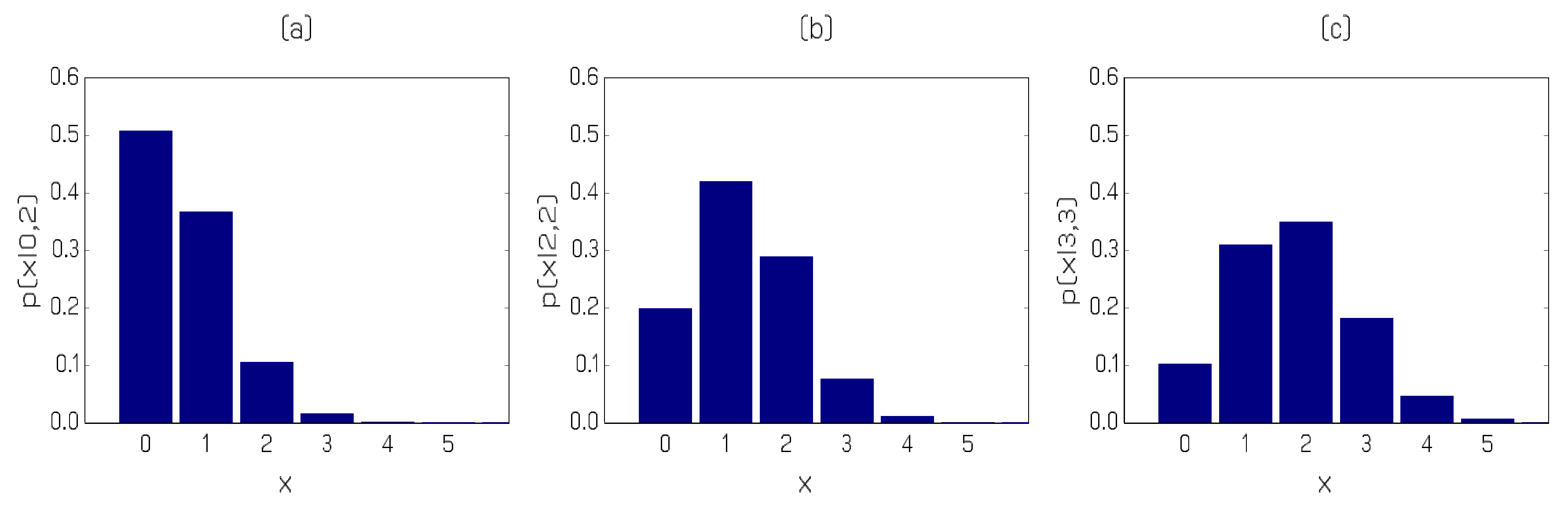
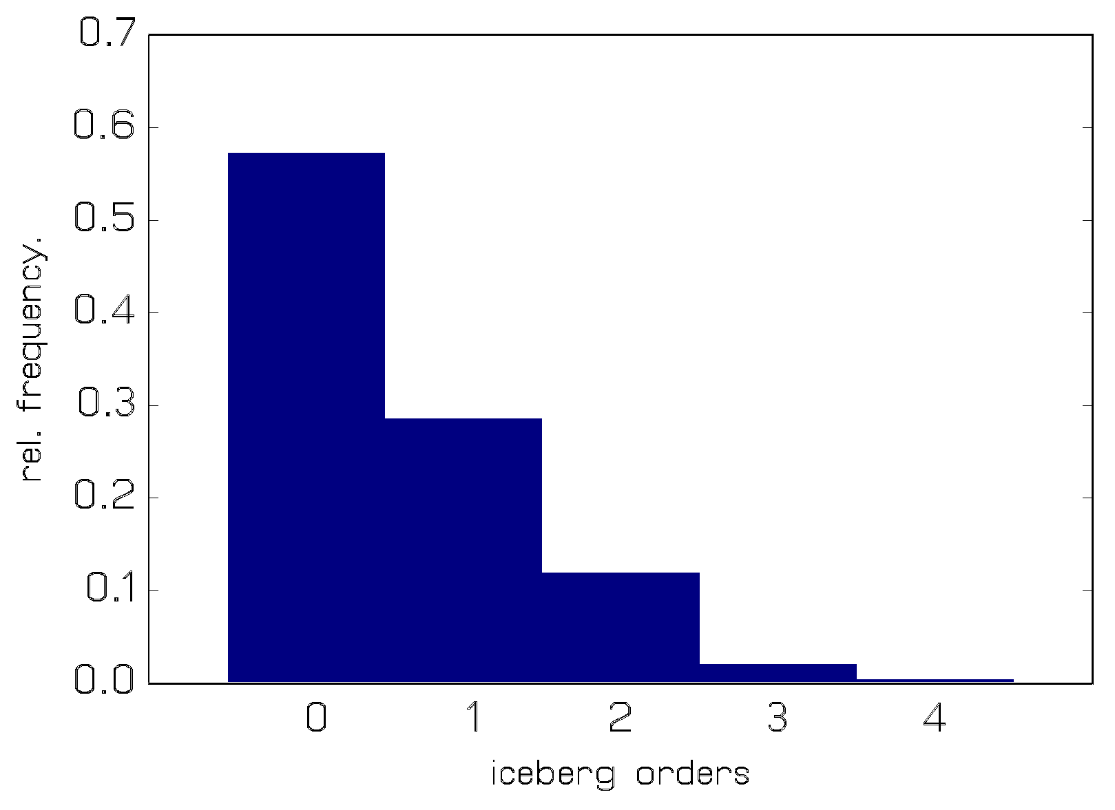
In this section we demonstrate the applicability of the PAR(2)-AA model to a real-world data set. We consider iceberg order data from the ask side of the Lufthansa stock sampled from the XETRA trading system at a frequency of 15 minutes during 15 consecutive trading days in the first quarter of 2004. For some explanatory remarks about the nature of iceberg orders, see e.g., Jung and Tremayne (2011). The sample consists of 510 (low) counts ranging from 0 to 4. The marginal distribution of the counts is shown in Figure 2; the sample mean and variance of the data are, respectively, 0.616 and 0.673. A time series plot and the sample (partial) autocorrelations (S(P)ACFs) are depicted in Figure 3.
The time series plot of the data shows no discernable trend, the sample mean and variance do not suggest overdispersion and the SACF and SPACF of the data point toward a first or second order autoregressive dynamic structure. Based on these findings we fit a PAR(1) and a PAR(2)-AA model to the first 505 observations, with the last five reserved for an illustrative out-of-sample prediction exercise.
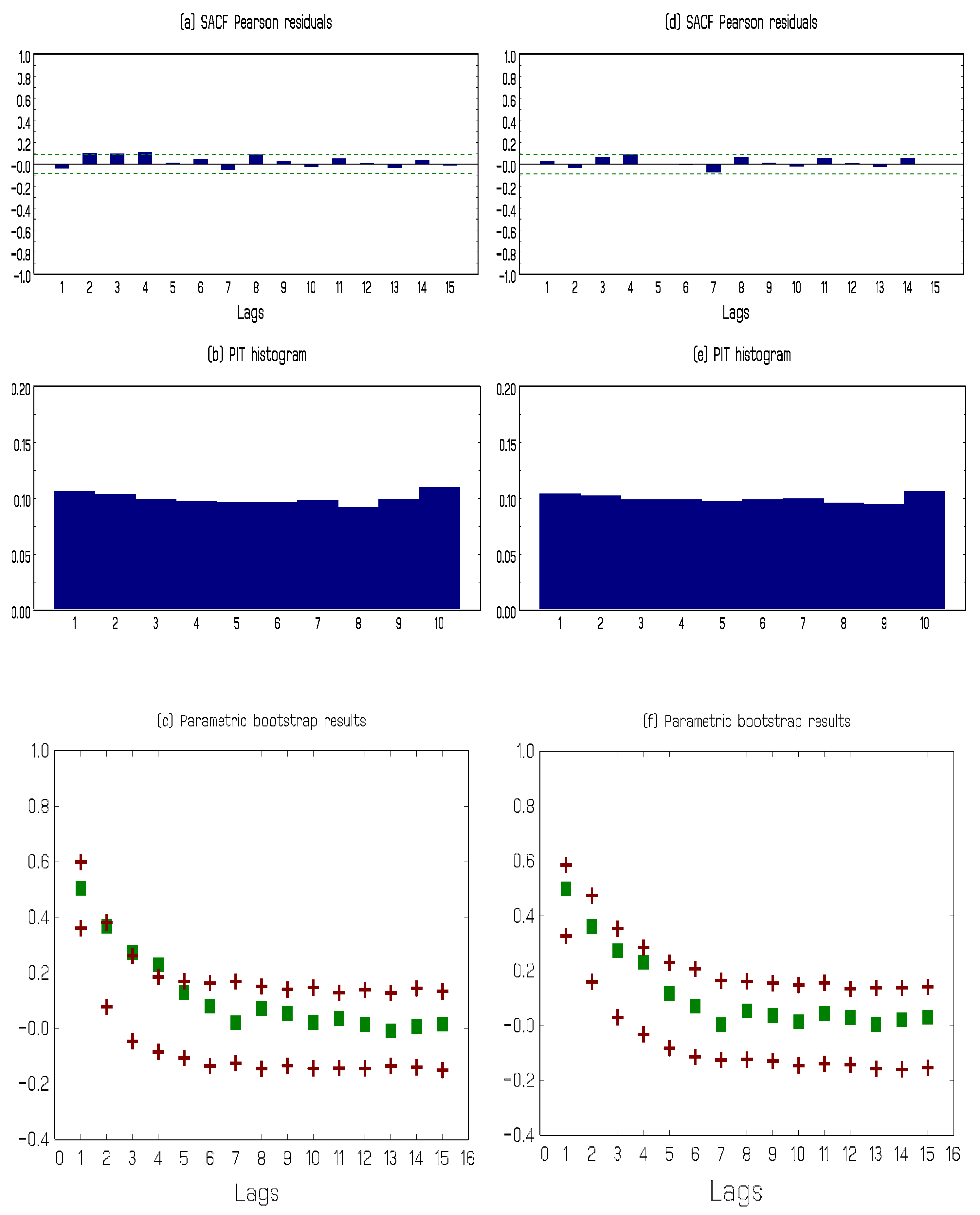
To compare the two model fits, we exploit goodness-of-fit techniques based on: (a) the predictive distributions of the two models, in particular the PIT histogram and scoring rules; (b) the correlogram of the Pearson residuals computed as ; and (c) a parametric resampling procedure based on Tsay (1992). See Jung et al. (2016) and Czado et al. (2009) for more details. Figure 4 depicts the results for the two fitted models.
It is evident from the panels in Figure 4 that the fit of the PAR(2)-AA model is superior to that of the PAR(1) model, certainly when it comes to capturing the serial dependence in the data. Further evidence favouring the PAR(2)-AA specification is provided by comparing the scoring rules provided in Table 5 for the two model fits. We, therefore, report parameter estimates and out-of-sample results for the preferred second order model only.
Table 6 provides the parameter estimates for the three parameters of the PAR(2)-AA model based on method of moments, NLS, GMM and ML estimation, respectively. Estimated standard errors are provided for the ML estimates only. It is evident that the parameter estimate for the parameter is statistically different from zero, providing further statistical evidence of a preference for the PAR(2)-AA model over the PAR(1) one.
We now present an illustration of out-of-sample prediction for the PAR(2)-AA model. We employ a fixed forecasting environment using only the fit to observations 1 to 505. Observations 504 to 510 are, in fact, (2,0,2,2,3,3,2); since a value 3 is only observed of times in the entire realization, these data represent a short epoch of values that will perforce be difficult to forecast. Using (12) we select three predictive distributions with different Markovian histories (pairs of lagged counts) for graphical presentation in Figure 5. Panel (a) in the Figure corresponds to the prediction of observation number 506 (observed value 2, relevant past history 2,0); the predictive distribution has a mode of zero with an estimated probability close to so that the observed value of 2 is seen as unlikely, having a predicted probability of around . In Panel (b) of the Figure, the predictive distribution for observation number 508 is provided (observed value 3, relevant past history 2,2). The predictive distribution for the one-step ahead forecast is now markedly different; the mode has shifted up to 1, the probability of observing another 2 has risen to and even the large value of 3 is forecast to occur with estimated probability . Finally, Panel (c) portrays the predictive distribution for observation 510 (observed value 2 with relevant past history 3,3). Note that the estimated probability of observing yet another 3 has risen to about and the modal forecast is in fact the value observed. Overall, the three panels of the Figure illustrate clearly how rapidly the predictive distribution responds to altering relevant past history.
6. Concluding Remarks
This paper considers maximum likelihood estimation in an integer autoregressive model for which such parameter estimators have not been available hithero. The basic techniques used are reduction methods and change of variable techniques. The expressions that emerge for the conditional (predictive) distributions are complicated involving, as they do, multiple summations. We demonstrate that they can be fruitfully used for inferential purposes using a real-world data set. Moreover, the predictive distributions derived can be employed in goodness-of-fit analyses and out-of-sample predictions leading to probabilistic forecasts.
Author Contributions
Both authors have contributed equally to all aspects of the preparation and writing of this paper. They have both read and agreed to the published version of the manuscript.
Funding
This research received no external funding.
Acknowledgments
We are grateful to two anonymous Referees whose comments led to improvements to the original version of the paper. In particular, the simulation evidence relating to GMM estimation stemmed from one such suggestion.
Conflicts of Interest
The authors declare no conflict of interest.
References
- Al-Osh, M. A., and A. A. Alzaid. 1987. First-order integer-valued autoregressive (INAR (1)) process. Journal of Time Series Analysis 8: 261–75. [Google Scholar] [CrossRef]
- Alzaid, A. A., and M. Al-Osh. 1990. An integer-valued pth-order autoregressive structure (INAR(p)) process. Journal of Applied Probability 27: 314–23. [Google Scholar] [CrossRef]
- Brännäs, Kurt. 1994. Estimation and Testing in Integer-Valued AR(1) Models. University of Umeå Discussion Paper No. 335. Umeå: University of Umeå. [Google Scholar]
- Bu, Ruijun, Kaddour Hadri, and Brendan P. M. McCabe. 2008. Maximum likelihood estimation of higher-order integer-valued autoregressive processes. Journal of Time Series Analysis 29: 973–94. [Google Scholar] [CrossRef]
- Consul, P. C. 1989. Generalized Poisson Distributions: Properties and Applications. New York: Marcel Dekker. [Google Scholar]
- Czado, Claudia, Tilmann Gneiting, and Leonhard Held. 2009. Predictive model assessment for count data. Biometrics 65: 1254–61. [Google Scholar] [CrossRef] [PubMed]
- Drost, Feike C., Ramon van den Akker, and Bas J. M. Werker. 2009. Efficient estimation of auto-regression parameters and innovation distributions for semiparametric integer-valued AR(p) models. Journal of the Royal Statistical Society, Series B 71: 467–85. [Google Scholar] [CrossRef]
- Du, Jin-Guan, and Yuan Li. 1991. The integer-valued autoregressive (INAR (p)) model. Journal of Time Series Analysis 12: 129–42. [Google Scholar]
- Hansen, Lars Peter. 1982. Large sample properties of generalized method of moments estimators. Econometrica 50: 1029–54. [Google Scholar] [CrossRef]
- Joe, Harry. 1996. Time series models with univariate margins in the convolution-closed infinitely divisible class. Journal of Applied Probability 33: 664–77. [Google Scholar] [CrossRef]
- Jung, Robert C., Brendan P. M. McCabe, and Andrew R. Tremayne. 2016. Model validation and diagonostics. In Handbook of Discrete-Valued Time Series. Edited by Richard A. Davis, Scott H. Holan, Robert Lund and Nalini Ravishanker. Boca Raton: CRC Press, pp. 189–218. [Google Scholar]
- Jung, Robert C., Gerd Ronning, and Andrew R. Tremayne. 2005. Estimation in conditional first order autoregression with discrete support. Statistical Papers 46: 195–224. [Google Scholar] [CrossRef]
- Jung, Robert C., and Andrew R. Tremayne. 2003. Testing for serial dependence in time series of counts. Journal of Time Series Analysis 24: 65–84. [Google Scholar] [CrossRef]
- Jung, Robert C., and Andrew R. Tremayne. 2006. Coherent forecasting in integer time series models. International Journal of Forecasting 22: 223–38. [Google Scholar] [CrossRef]
- Jung, Robert C., and Andrew R. Tremayne. 2011. Convolution-closed models for count time series with applications. Journal of Time Series Analysis 32: 268–80. [Google Scholar] [CrossRef]
- Karlis, Dimitris. 2003. An EM algorithm for multivariate Poisson distribution and related models. Journal of Applied Statistics 30: 63–77. [Google Scholar] [CrossRef]
- Loukas, S., and C. D. Kemp. 1983. On computer sampling from trivariate and multivariate discrete distributions. Journal of Statistical Compuation and Simulation 17: 113–23. [Google Scholar] [CrossRef]
- Mahamunulu, D. M. 1967. A note on regression in the multivariate Poisson distribution. Journal of the American Statistical Association 62: 251–58. [Google Scholar] [CrossRef]
- Mardia, K. V. 1970. Families of Bivariate Distributions. London: Charles Griffin & Co. [Google Scholar]
- Martin, Gael, Brendan P. M. McCabe, and David Harris. 2011. Optimal probabalistic forecasts for counts. Journal of the Royal Statistical Society: Series B 73: 253–72. [Google Scholar]
- McKenzie, Ed. 1985. Some simple models for discrete variate time series. Water Resources Bulletin 21: 645–50. [Google Scholar] [CrossRef]
- McKenzie, Ed. 1988. Some ARMA models for dependent sequences of Poisson counts. Advances in Applied Probability 20: 822–35. [Google Scholar] [CrossRef]
- Schweer, Sebastian. 2015. On the time-reversibility of integer-valued autoregressive processes of general order. In Stochastic Models, Statistics and Their Applications. Edited by Ansgar Steland, Ewaryst Rafajłowicz and Krzysztof Szajowski. Cham: Springer International Publishing, pp. 169–77. [Google Scholar]
- Silva, Isabel, Maria Eduarda Silva, and Cristina Torres. 2020. Inference for bivariate integer-valued moving average models based on binomial thinning operation. Journal of Applied Statistics. [Google Scholar] [CrossRef]
- Steutel, Fred W., and Klaas van Harn. 1979. Discrete analogues of self-decomposability and stability. The Annals of Probability 7: 893–99. [Google Scholar] [CrossRef]
- Tsay, Ruey S. 1992. Model checking via parametric bootstraps in time series analysis. Applied Statistics 41: 1–15. [Google Scholar] [CrossRef]
Figure 1.
Partition of the parameter space in the PAR(2)-AA model.
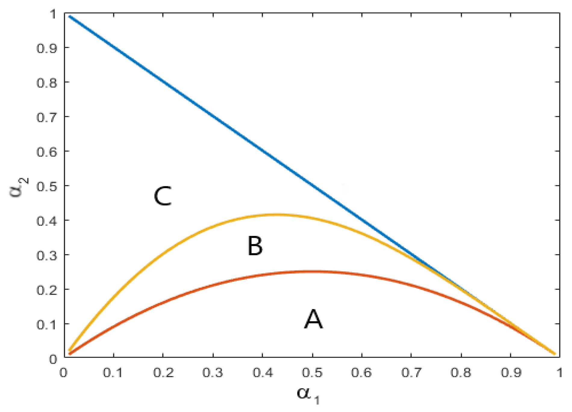
Figure 2.
Marginal distribution of the iceberg order data.

Figure 3.
Time series plot (panel (a)) and SACF and SPACF (panels (b,c)) of the iceberg order data.

Figure 4.
PAR(1) model fit: residual autocorrelations (panel (a)), PIT histogram (panel (b)) and parametric resampling procedure (panel (c)); Panels (d–f) depict the corresponding information for the PAR(2)-AA model fit.
Figure 4.
PAR(1) model fit: residual autocorrelations (panel (a)), PIT histogram (panel (b)) and parametric resampling procedure (panel (c)); Panels (d–f) depict the corresponding information for the PAR(2)-AA model fit.

Figure 5.
One-step ahead predictive distributions of the iceberg order data based on the PAR(2)-AA model.
Figure 5.
One-step ahead predictive distributions of the iceberg order data based on the PAR(2)-AA model.

Table 1.
Bias, percentage bias and MSE for the MM, NLS, GMM and ML parameter estimates for the first set of simulation experiments.
Table 1.
Bias, percentage bias and MSE for the MM, NLS, GMM and ML parameter estimates for the first set of simulation experiments.
| T = 125 | T = 250 | T = 500 | |||||||
|---|---|---|---|---|---|---|---|---|---|
| Bias | % Bias | MSE | Bias | % Bias | MSE | Bias | % Bias | MSE | |
| −0.0184 | −6.1295 | 0.0095 | −0.0082 | −2.7190 | 0.0048 | −0.0031 | −1.0299 | 0.0024 | |
| 0.0060 | 6.0003 | 0.0045 | −0.0026 | −2.5795 | 0.0027 | −0.0045 | −4.5395 | 0.0016 | |
| 0.0381 | 2.1182 | 0.1259 | 0.0306 | 1.7013 | 0.0665 | 0.0239 | 1.3274 | 0.0357 | |
| −0.0181 | −6.0494 | 0.0097 | −0.0081 | −2.6876 | 0.0048 | −0.0030 | −0.9976 | 0.0024 | |
| 0.0059 | 5.9088 | 0.0044 | −0.0022 | −2.2255 | 0.0026 | −0.0043 | −4.3151 | 0.0015 | |
| 0.0374 | 2.0780 | 0.1288 | 0.0294 | 1.6359 | 0.0663 | 0.0227 | 1.2613 | 0.0350 | |
| 0.0017 | 0.5772 | 0.0081 | 0.0008 | 0.2833 | 0.0042 | 0.0012 | 0.4130 | 0.0020 | |
| 0.0163 | 16.2588 | 0.0052 | 0.0034 | 3.4103 | 0.0029 | −0.0020 | −2.0000 | 0.0017 | |
| −0.0760 | −4.2202 | 0.1463 | −0.0269 | −1.4919 | 0.0743 | −0.0037 | −0.2059 | 0.0382 | |
| −0.0091 | −3.0481 | 0.0079 | −0.0038 | −1.2681 | 0.0039 | −0.0009 | −0.3133 | 0.0019 | |
| 0.0092 | 9.1655 | 0.0046 | −0.0006 | −0.6137 | 0.0026 | −0.0034 | −3.3661 | 0.0015 | |
| 0.0004 | 0.0231 | 0.1095 | 0.0123 | 0.6835 | 0.0567 | 0.0138 | 0.7659 | 0.0350 | |
Table 2.
Bias, percentage bias and MSE for the MM, NLS, GMM and ML parameter estimates for the second set of simulation experiments.
Table 2.
Bias, percentage bias and MSE for the MM, NLS, GMM and ML parameter estimates for the second set of simulation experiments.
| T = 125 | T = 250 | T = 500 | |||||||
|---|---|---|---|---|---|---|---|---|---|
| Bias | % Bias | MSE | Bias | % Bias | MSE | Bias | % Bias | MSE | |
| −0.0398 | −9.9578 | 0.0161 | −0.0234 | −5.8488 | 0.0081 | −0.0120 | −3.0109 | 0.0041 | |
| −0.0218 | −7.2567 | 0.0067 | −0.0096 | −3.1834 | 0.0031 | −0.0046 | −1.5190 | 0.0015 | |
| 0.2397 | 19.9773 | 0.3230 | 0.1295 | 10.7939 | 0.1453 | 0.0643 | 5.3613 | 0.0656 | |
| −0.0359 | −8.9634 | 0.0158 | −0.0202 | −5.0405 | 0.0078 | −0.0107 | −2.6808 | 0.0036 | |
| −0.0196 | −6.5475 | 0.0066 | −0.0082 | −2.7461 | 0.0031 | −0.0039 | −1.3010 | 0.0015 | |
| 0.2142 | 17.8467 | 0.3097 | 0.1101 | 9.1726 | 0.1347 | 0.0562 | 4.6809 | 0.0595 | |
| −0.0196 | −4.8996 | 0.0114 | −0.0177 | −4.4334 | 0.0062 | −0.0173 | −4.3301 | 0.0032 | |
| −0.0125 | −4.1821 | 0.0075 | −0.0040 | −1.3494 | 0.0037 | −0.0018 | −0.6145 | 0.0019 | |
| 0.0622 | 5.1825 | 0.1534 | 0.0481 | 4.0122 | 0.0765 | 0.0392 | 3.2707 | 0.0394 | |
| −0.0102 | −2.5588 | 0.0090 | −0.0053 | −1.3262 | 0.0044 | −0.0026 | −0.6381 | 0.0021 | |
| −0.0124 | −4.1226 | 0.0058 | −0.0043 | −1.4382 | 0.0028 | −0.0016 | −0.5326 | 0.0014 | |
| 0.0830 | 6.9171 | 0.1238 | 0.0351 | 2.9239 | 0.0525 | 0.0144 | 1.2041 | 0.0252 | |
Table 3.
Bias, percentage bias and MSE for the MM, NLS, GMM and ML parameter estimates for the third set of simulation experiments.
Table 3.
Bias, percentage bias and MSE for the MM, NLS, GMM and ML parameter estimates for the third set of simulation experiments.
| T = 125 | T = 250 | T = 500 | |||||||
|---|---|---|---|---|---|---|---|---|---|
| Bias | % Bias | MSE | Bias | % Bias | MSE | Bias | % Bias | MSE | |
| −0.0337 | −11.2201 | 0.0172 | −0.0208 | −6.9254 | 0.0100 | −0.0128 | −4.2741 | 0.0052 | |
| −0.0303 | −7.5864 | 0.0076 | −0.0149 | −3.7346 | 0.0035 | −0.0065 | −1.6159 | 0.0017 | |
| 0.2490 | 20.7534 | 0.3556 | 0.1379 | 11.4933 | 0.1775 | 0.0756 | 6.3016 | 0.0839 | |
| −0.0299 | −9.9535 | 0.0165 | −0.0171 | −5.7006 | 0.0093 | −0.0103 | −3.4362 | 0.0943 | |
| −0.0280 | −7.0074 | 0.0074 | −0.0135 | −3.3785 | 0.0035 | −0.0057 | −1.4359 | 0.0017 | |
| 0.2218 | 18.4864 | 0.3319 | 0.1164 | 9.7004 | 0.1603 | 0.0621 | 5.1726 | 0.0728 | |
| −0.0322 | 10.7468 | 0.0158 | −0.0188 | −6.2515 | 0.0106 | −0.0093 | −3.1356 | 0.0897 | |
| −0.0189 | 4.7178 | 0.0077 | −0.0038 | −0.9412 | 0.0038 | −0.0023 | −0.5643 | 0.0017 | |
| −0.1098 | 0.1531 | 0.2068 | 0.1030 | 8.5847 | 0.1195 | 0.0432 | 3.5785 | 0.0410 | |
| −0.0100 | −3.3439 | 0.0121 | −0.0053 | −1.7654 | 0.0065 | −0.0036 | −1.2038 | 0.0032 | |
| −0.0176 | −4.4007 | 0.0062 | −0.0071 | −1.7631 | 0.0031 | −0.0022 | −0.5419 | 0.0015 | |
| 0.1001 | 8.344 | 0.1475 | 0.0436 | 3.6343 | 0.0694 | 0.0213 | 1.7727 | 0.0313 | |
Table 4.
Bias, percentage bias and MSE for the MM, NLS, GMM and ML parameter estimates for the fourth set of simulation experiments.
Table 4.
Bias, percentage bias and MSE for the MM, NLS, GMM and ML parameter estimates for the fourth set of simulation experiments.
| T = 125 | T = 250 | T = 500 | |||||||
|---|---|---|---|---|---|---|---|---|---|
| Bias | % Bias | MSE | Bias | % Bias | MSE | Bias | % Bias | MSE | |
| −0.0340 | −6.8063 | 0.0181 | −0.0181 | −3.6114 | 0.0058 | −0.0078 | −1.5659 | 0.0029 | |
| 0.0069 | 6.9004 | 0.0045 | −0.0019 | −1.8796 | 0.0026 | −0.0033 | −3.2875 | 0.0016 | |
| 0.0140 | 5.8252 | 0.0059 | 0.0102 | 4.2585 | 0.0032 | 0.0052 | 2.1674 | 0.0015 | |
| −0.0321 | −6.4257 | 0.0119 | −0.0172 | −3.4276 | 0.0057 | −0.0077 | −1.5303 | 0.0028 | |
| 0.0059 | 5.9070 | 0.0043 | −0.0012 | −1.1918 | 0.0023 | −0.0020 | −2.0464 | 0.0013 | |
| 0.0125 | 5.1238 | 0.0019 | 0.0087 | 3.6118 | 0.0029 | 0.0043 | 1.7753 | 0.0014 | |
| −0.0085 | −1.7007 | 0.0118 | −0.0032 | −0.6340 | 0.0040 | −0.0016 | −0.3230 | 0.0020 | |
| 0.0168 | 16.8447 | 0.0045 | 0.0034 | 3.4105 | 0.0029 | −0.0019 | −1.8700 | 0.0017 | |
| −0.0079 | −5.8751 | 0.0059 | −0.0027 | −1.1208 | 0.0025 | 0.0006 | 0.2445 | 0.0014 | |
| −0.0144 | −2.8759 | 0.0072 | −0.0068 | −1.2115 | 0.0034 | −0.0032 | −0.6359 | 0.0016 | |
| 0.0041 | 4.0920 | 0.0035 | −0.0009 | −0.0728 | 0.0019 | −0.0014 | −1.4325 | 0.0010 | |
| 0.0026 | 1.0681 | 0.0035 | 0.0023 | 0.6756 | 0.0017 | 0.0012 | 0.4976 | 0.0009 | |
Table 5.
Scoring rules for the PAR(1) and the PAR(2)-AA model fit.
| Scoring Rule | PAR(1) | PAR(2)-AA |
|---|---|---|
| log score | 0.9174 | 0.9058 |
| quadratic score | 0.5161 | 0.5081 |
| ranked prob. score | 0.3315 | 0.3258 |
Table 6.
Parameter estimates for the iceberg order data based on the PAR(2)-AA model.
| Parameter | MM Estimates | NLS Estimates | GMM Estimates | ML Estimates | ML Standard Errors |
|---|---|---|---|---|---|
| 0.4990 | 0.4954 | 0.4712 | 0.4668 | 0.0410 | |
| 0.1147 | 0.0924 | 0.0806 | 0.0999 | 0.0349 | |
| 0.2310 | 0.2485 | 0.2759 | 0.2614 | 0.0296 |
© 2020 by the authors. Licensee MDPI, Basel, Switzerland. This article is an open access article distributed under the terms and conditions of the Creative Commons Attribution (CC BY) license (http://creativecommons.org/licenses/by/4.0/).
Share and Cite
MDPI and ACS Style
Jung, R.C.; Tremayne, A.R. Maximum-Likelihood Estimation in a Special Integer Autoregressive Model. Econometrics 2020, 8, 24. https://0-doi-org.brum.beds.ac.uk/10.3390/econometrics8020024
AMA Style
Jung RC, Tremayne AR. Maximum-Likelihood Estimation in a Special Integer Autoregressive Model. Econometrics. 2020; 8(2):24. https://0-doi-org.brum.beds.ac.uk/10.3390/econometrics8020024
Chicago/Turabian StyleJung, Robert C., and Andrew R. Tremayne. 2020. "Maximum-Likelihood Estimation in a Special Integer Autoregressive Model" Econometrics 8, no. 2: 24. https://0-doi-org.brum.beds.ac.uk/10.3390/econometrics8020024
Note that from the first issue of 2016, this journal uses article numbers instead of page numbers. See further details here.