Frequency-Domain Evidence for Climate Change

Department of Statistics and Operations Research, University of Vienna, Oskar-Morgenstern-Platz 1, 1090 Vienna, Austria
*
Author to whom correspondence should be addressed.
Econometrics 2020, 8(3), 28; https://0-doi-org.brum.beds.ac.uk/10.3390/econometrics8030028
Submission received: 13 February 2020
/
Revised: 15 July 2020
/
Accepted: 15 July 2020
/
Published: 20 July 2020
(This article belongs to the Collection Econometric Analysis of Climate Change)
Abstract
:The goal of this paper is to search for conclusive evidence against the stationarity of the global air surface temperature, which is one of the most important indicators of climate change. For this purpose, possible long-range dependencies are investigated in the frequency-domain. Since conventional tests of hypotheses about the memory parameter, which measures the degree of long-range dependence, are typically based on asymptotic arguments and are therefore of limited practical value in case of small or medium sample sizes, we employ a new small-sample test as well as a related estimator for the memory parameter. To safeguard against false positive findings, simulation studies are carried out to examine the suitability of the employed methods and hemispheric datasets are used to check the robustness of the empirical findings against low-frequency natural variability caused by oceanic cycles. Overall, our frequency-domain analysis provides strong evidence of non-stationarity, which is consistent with previous results obtained in the time domain with models allowing for stochastic or deterministic trends.
Keywords:
global warming; fractionally integrated processes; stationarity test; frequency-domain test; frequency-domain estimatorsJEL Classification:
Q54; C12; C141. Introduction
While the presence of global warming is largely undisputed among experts and public climate change awareness has reached levels of over in Western countries (Lee et al. 2015; Poortinga et al. 2018; Baiardi and Morana 2020), the verification of a change in the global surface temperature in terms of statistical significance remains a challenging task. The main problem is that there is no consensus about the true nature of the underlying process which has generated the observed temperature record. It may have a deterministic trend, a stochastic trend or even a combination of both. It may also share its trend in certain subperiods with other time series such as greenhouse gas emissions, which would allow us to draw conclusions about the cause of the warming trend. In order to address questions of this type, various sophisticated time series models have been employed in previous studies, a selection of which will be reviewed in Section 1. However, when we are only interested in the question whether the global surface temperature is changing or not, we may be able to choose a relatively simple setting and possibly avoid to impose implausibly strong assumptions.
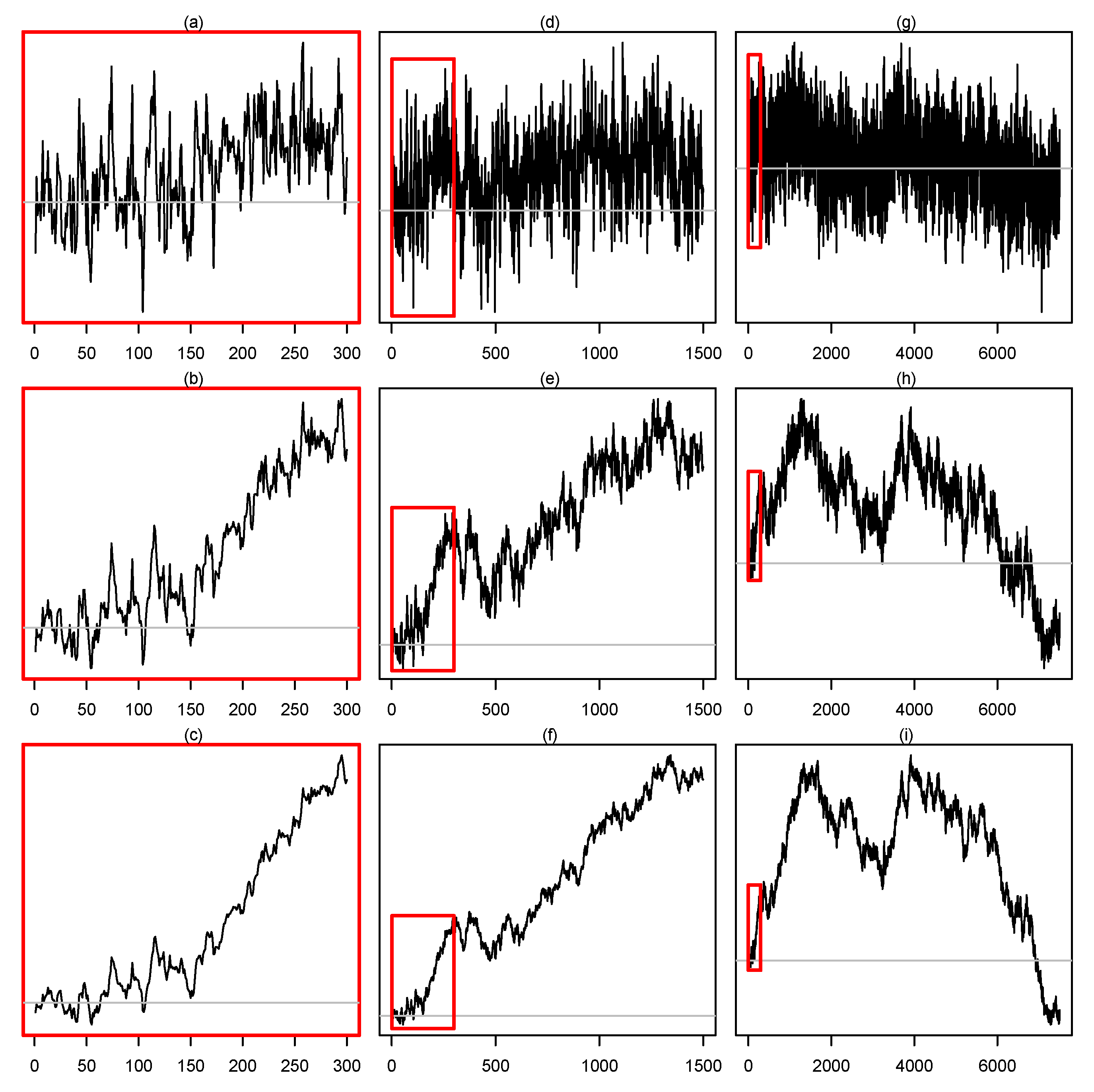
In this paper, we consider only fractionally integrated processes with constant mean, and try to distinguish between the stationary case, where the memory parameter d is less than 0.5, and the non-stationary case, where . In this setting, the rejection of the stationarity hypothesis can always be interpreted as evidence of climate change, regardless whether the rejection is due to a large value of d (infinite variance) or a nonconstant mean (deterministic trend). To emphasize the importance of including the non-stationary, yet mean-reverting case in the alternative hypothesis of climate change, we plotted realizations of fractional white noise for different values of d and different sample sizes. Figure 1g shows that even for a relatively large value of d in the stationary range, the long-term fluctuations are modest. In contrast, the changes are quite dramatic for .
See Figure 1h. Changes of this magnitude would be disastrous in the case of the global temperature.
However, when testing the hypothesis , we have to strike a balance between simplicity and plausibility. On the one hand, we must allow for short-range dependence in order to keep the test realistic, hence using only fractionally integrated white noise is not an option. On the other hand, the class of data generating processes (DGPs) must also not be too rich because Pötscher (2002) has shown that inference on unit roots and cointegration as well as the problem of estimating the memory parameter fall into the category of ill-posed estimation problems under commonly used specifications for the set of feasible DGPs. For example, reliable unit root inference is not possible when this set is rich enough to contain all ARMA(1, 1) processes.
Conventional tests of hypotheses about the memory parameter d are based on the asymptotic normality of semiparametric estimators for d which are obtained from the periodogram ordinates at Fourier frequencies in a small neighborhood of frequency zero. The restriction to consider only the lowest Fourier frequencies certainly helps to avoid any distortions caused by short-range dependencies but it also compromises the large-sample assumption required for the asymptotics to kick in. Mangat and Reschenhofer (2019) therefore developed a small-sample test which requires only that the total sample size is large but not the number Fourier frequencies that are used in the test procedure. Building on this test, Reschenhofer and Mangat (2020) introduced a new estimator for d, which performed well in terms of bias and root-mean-square error (RMSE) in an extensive simulation study. Both the test and the estimator will be used together with other methods in Section 3 to search for conclusive evidence against the stationarity of the global air surface temperature. Before, in Section 2, all employed methods will be described in detail. Section 4 concludes the paper.
Literature Review
A popular way to test for a trend in a time series is based on the simple linear trend model. Under the assumption that the errors are stationary with mean zero and variance , the OLS estimator for the slope parameter is in case of a large sample size n approximately normally distributed with mean and variance (Grenander and Rosenblatt 1957). Using the fact that the error variance is proportional to the spectral density of the error process at frequency zero, it can be estimated by a suitable lag window estimator based on the sample autocovariances of the OLS residuals. However, as pointed out by Fomby and Vogelsang (2002), this approach breaks down when there is a unit root in the errors or the errors have long memory because in these cases the spectral density at frequency zero does not exist. In their analysis of six global temperature series, Fomby and Vogelsang (2002) therefore used the robust trend test proposed by Vogelsang (1998) instead and were able to reject the null hypothesis of a nonpositive linear trend at the level in all but one case. The robustness of this test to strong serial correlation implies that it cannot be used for the detection of a stochastic trend, hence other tests must be used for this purpose.
Using various unit root tests to test for the presence of stochastic trends in three temperature series (northern hemisphere, southern hemisphere, global; period: 1865–1994), Stern and Kaufmann (1999) obtained conflicting results. The augmented Dickey–Fuller (ADF) test (Dickey and Fuller 1979, 1981) and the Kwiatowski–Phillips–Schmidt–Shin (KPSS) test (Kwiatkowski et al. 1992) suggested that all temperature series are (integrated of order one), which means that they require differencing to achieve stationarity, whereas the Phillips–Perron test (Phillips and Perron 1988) and the Schmidt–Phillips test (Schmidt and Phillips 1992) suggested that all temperature series are I(0) (trend stationary), which means that the subtraction of a deterministic trend is sufficient to achieve stationarity. Taking also the spatial distribution of the temperature into account, Chang et al. (2020) detected functional unit roots in time series of cross-sectional temperature densities.
Once we have established that surface temperature follows a stochastic trend, we might go one step further and investigate the causes for the changes in surface temperature. This could be done by testing whether surface temperature cointegrates with independent variables like greenhouse gases. The existence of a cointegrating relationship would indicate that there is a common stochastic trend and consequently also that human activity is responsible for the rising temperature. However, the methodological problems do not become any smaller when we move from a univariate analysis to a multivariate analysis. Indeed, the reports of cointegrating relationships by Kaufmann and Stern (2002) and Kaufmann et al. (2006) were challenged by Gay-Garcia et al. (2009) who argued that surface temperature is stationary around a broken linear trend. Kaufmann et al. (2010) responded that the in-sample forecasts generated by the cointegration model are more accurate than the in-sample forecast generated by the broken trend model. Conceding that a single break may not be enough for the rejection of non-stationarity, Lai and Yoon (2018) tried up to three breaks and were then able to reject the unit root hypothesis in favor of stationarity about a broken trend for both global and hemispheric temperatures. They used the unit root test proposed by Harvey et al. (2013), which extends the minimum GLS detrended Dickey—Fuller (MDF) test of Perron and Rodríguez (2003) by allowing for multiple breaks.
However, the evidence presented by Lai and Yoon (2018) must be interpreted with caution. Firstly, in relation to the modest sample size of (observation period from 1880 to 2015) there are simply too many tuning parameters besides the maximum number of breaks, namely the trimming parameters determining the times and of the earliest possible break and the latest possible break, respectively, the separation parameter determining the minimum number of observations between breaks, and the number p of lags used in the ADF-type autoregression or the maximum number of lags if p is chosen automatically, e.g., by the modified Akaike information criterion (MAIC) procedure of Ng and Perron (2001) and Perron and Qu (2007). Moreover, Lai and Yoon (2018) also considered three different types of breaks occurring either in the intercept, in the slope, or both in the intercept and the slope. Less problematic are the specifications required for the calculation of the asymptotic critical values because they leave no room for data snooping when the values provided by Harvey et al. (2013) are used. Secondly, the underlying asymptotics of this test is intuitively not very plausible. Suppose that three breaks in 150 years are a realistic estimate, then we would expect six breaks in 300 years and 30 breaks in 1500 years. Why should the maximum number of breaks remain fixed when the sample size increases? This can only happen when we keep the length of the observation period fixed and increase only the sampling frequency. For example, when we switch from annual observations to weekly observations, the sample size n increases dramatically from n to but the number of breaks does not change and the minimum number of observations between breaks increases accordingly from to . Clearly, this kind of asymptotics is inappropriate for the investigation of climate change. Not much new can be learned about the long-term trend of the global surface temperature when weekly, daily or hourly measurements are used instead of annual measurements. Unfortunately, the “right asymptotics”, where the number of breaks grows at the same rate as the length of the observation period, does not appear to be a practical option.
Instead of assuming that surface temperature and greenhouse gases have stochastic trends and searching for evidence of a cointegrating relationship, we may as well assume trend-stationarity and search for a common deterministic trend in order to establish that human factors are responsible for the rising temperature. Estrada et al. (2013) provided evidence for the existence of such a trend, which is characterized by common breaks in the slope. Perron and Yabu (2009) designed a test for structural breaks in a deterministic trend, which does not require any prior knowledge as to whether the deviations from the trend are difference- or trend-stationary. Applying this test to various temperature series (land and sea, global, northern and southern hemispheres) as well as series of greenhouse gases and other factors contributing to radiative forcing (difference of the sunlight absorbed by the Earth and the energy radiated back to space), Estrada et al. (2017) found breaks in the slope of the trend function in almost all series but also large differences in the break date estimates. They attributed these differences to natural variability, e.g., low-frequency oscillations such as the Atlantic Multidecadal Oscillation (AMO) and shorter-term variations such as El Nino/Southern Oscillation (ENSO). The results of cotrending analyses of Estrada et al. (2017) and Estrada and Perron (2019), which take the AMO into account, show that temperatures and forcing variables share the same long-term trend, which is highly influenced by greenhouse gases.
2. Methods
In light of the discussion in Section 1, we will employ low-order fractionally integrated ARMA (ARFIMA) models for the investigation of the long-range dependencies in the global surface temperature series. Our goal is to find conclusive evidence against the null hypothesis that the memory parameter d is less than 0.5. If , the variance will diverge and the time series will always tend to leave the previous range. Suppose that the observations can be described by an ARFIMA process
(Granger and Joyeux 1980; Hosking 1981), where L denotes the lag operator and is white noise with mean zero and variance . The memory parameter (or fractional differencing parameter) d is a measure of the degree of long-range dependence while the autoregressive parameters and the moving average parameters model the short-range dependence. Since we are only interested in long-range dependence and the ARMA-order is usually unknown anyway, we adopt a semiparametric approach and estimate d independently of the ARMA parameters. This can be achieved by carrying out the estimation in the frequency domain and focusing on the low frequency components. Indeed, the ARMA component
of the ARFIMA spectral density
is roughly constant for small values of and can therefore be approximated by
in a neighborhood of frequency zero. Frequency-domain estimators for d and frequency-domain tests of hypotheses about d will be discussed in Section 2.1 and Section 2.2, respectively, and later employed for the analysis of the temperature series in Section 3.
2.1. Estimation of the Memory Parameter
The periodogram is a sample version of the spectral density. It is given by
and is related to the sample autocovariances via
where
are the Fourier frequencies. Taking the logarithm of each side of (3) and adding the logarithm of the periodogram to both sides, we obtain
Since is approximately constant near frequency zero and the ratios , are asymptotically i.i.d. Exp(1), where Exp(1) denotes the exponential distribution with mean 1, if and (Künsch 1986), the memory parameter d can be estimated by a simple linear regression with as dependent variable and as independent variable (Geweke and Porter-Hudak 1983). The resulting estimator for d is denoted as when the K lowest Fourier frequencies are included in the regression and as when the H very lowest Fourier frequencies are trimmed away.
Since the periodogram is a very volatile estimator for the spectral density, smoothing is an obvious option to boost its performance. Accordingly, we may replace the periodogram ordinates occurring in the log periodogram regression either by simple moving averages like or by the more sophisticated lag window estimator
(Hassler 1993; Peiris and Court 1993; Reisen 1994) where w is a lag window satisfying , and . A commonly used lag window is the Parzen window given by
In contrast to the last two estimators, which depend also on the additional tuning parameters H and m, respectively, the estimator depends only on the number K of included Fourier frequencies. It is obtained by maximization of the Whittle-likelihood in the narrow frequency band (Künsch 1987). An approximation of the Whittle-likelihood is given by
(Robinson 1995). Similarly the estimator is obtained by minimization of the test statistic of a two-sided Kolmogorov–Smirnov goodness-of fit test applied to the cumulative normalized periodogram
(Reschenhofer et al. 2020). This estimator is closely related to the small-sample test which will be described in the next subsection and which will be the most important tool in our empirical study of the temperature data.
2.2. Testing
The asymptotic normality
of the estimator established by Hurvich et al. (1998) under the assumption that and can be used to test hypotheses about the memory parameter d. The problem with this approach is that not only the sample size n must be large but also the number K of included Fourier frequencies. A popular choice for K is . The length of our temperature series is 170, hence , which is definitely not a large number. Alternatively, we may also use the standard variance formula of the least squares estimator of the slope in a simple linear regression instead of the asymptotic variance. However, Mangat and Reschenhofer (2019) found that the test based on the asymptotic variance has very low power and the test based on the standard variance formula tends to over-reject under the null hypothesis. They therefore developed a new frequency-domain test which works also when K is small.
Their test is based on the assumption that a relatively small number of normalized periodogram ordinates at low Fourier frequencies are approximately i.i.d. Exp(1), possibly after omitting the very first frequencies, and consequently also that their cumulative sum is approximately distributed as the order statistics of a random sample from a uniform distribution on , which is plausible in the light of the asymptotic result by Künsch (1986) and the small-sample evidence provided by Mangat and Reschenhofer (2019). Clearly, the normalization requires the knowledge of the true value of d. If the value specified in the null hypothesis is wrong, there will be a discrepancy between the empirical distribution function of the sample, , and the cumulative distribution function of the uniform distribution, , which can be detected with a goodness-of-fit test like the Kolmogorv–Smirnov test. Compared to the small-sample test used by Reschenhofer (2013), this new test has the advantage that it allows for more general null hypotheses and does not require tables of critical values.
The empirical distribution function will be convex if the null hypothesis is false and concave if the reverse null hypothesis is false. Fortunately, these are exactly the cases where the Kolmogorov–Smirnov test is most powerful. Thus, we use the one-sided test based on the statistic
in order to reject the hypothesis when we suspect that . Analogously, we use the one-sided test based on the statistic
in order to reject the hypothesis when we suspect that . However, it is a priori not clear whether this test can also be employed in case of a null hypothesis such as , which requires the examination of the non-stationary borderline case . It will be shown in the next section how this can be done.
3. Empirical Results
Important theoretical results for the analysis of long-range dependence have typically been derived under the assumption , hence they cannot be used for the construction of tests of hypotheses such as and , which are the practically testable versions of the hypotheses of interest, and , respectively. Fortunately, there is a big difference between the two cases, which still allows us to get meaningful test results. For example, when we test the hypothesis instead of the hypothesis for the original time series, we clearly cannot interpret a rejection of that hypothesis as evidence against stationarity because the alternative hypothesis still contains the stationary region (0.4, 0.5). In contrast, when we test the hypothesis instead of the hypothesis for the differenced series, a rejection of that hypothesis implies that for the differenced series and consequently also that for the original series, which is strong evidence against stationarity. In our empirical study, we will therefore also have a closer look at the first differences of the temperature series.
The main datasets used in our investigation were the hemispheric and global annual means from 1850 to 2019 of the combined land and marine temperature anomalies (HadCRUT4; Morice et al. 2012), the land air temperature anomalies (CRUTEM4; see Jones et al. 2012), and the sea surface temperature anomalies (HadSST3; see Kennedy et al. 2011). These datasets were developed by the Climatic Research Unit of the University of East Anglia and the Met Office Hadley Centre and are available at the website http://www.cru.uea.ac.uk/. Temperature anomalies were defined relative to the 1961–1990 temperature mean. Secondary datasets were the NASA Goddard Institute for Space Studies (GISS) hemispheric annual means from 1880 to 2019, which are available at the website https://data.giss.nasa.gov/gistemp/ (Lenssen et al. 2019). In addition, we also use the annual unsmoothed (1856–2019) and smoothed (1861–2014) AMO series obtained by averaging from the corresponding monthly series, which are available at the website https://psl.noaa.gov/data/timeseries/AMO/ of the NOAA Physical Sciences Laboratory.
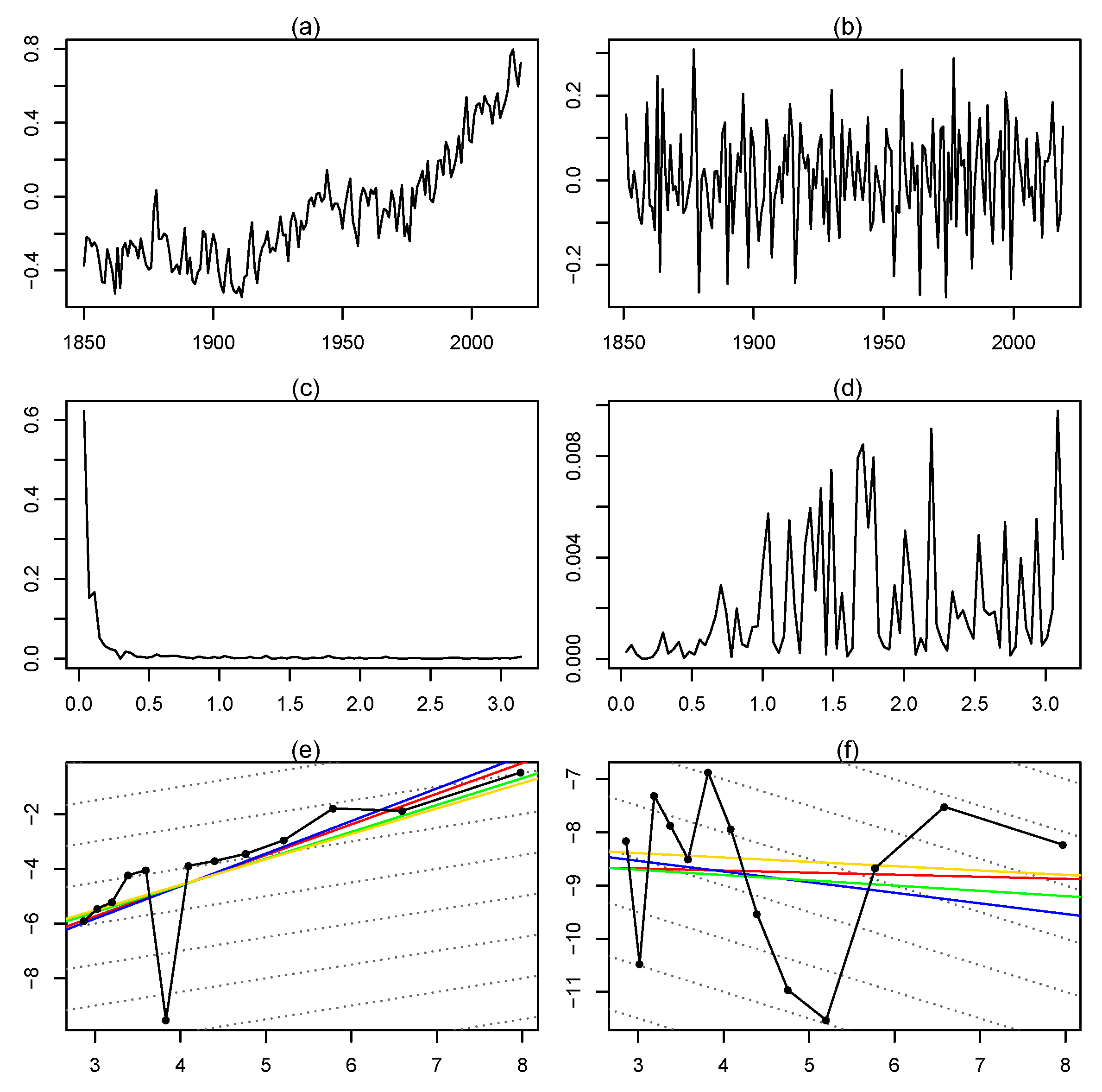
First, we looked at the global means of the combined land and marine temperature anomalies from the HadCRUT4 dataset. The central question was whether the clearly noticeable recent rise in temperature (see Figure 2a) is just a transient phenomenon or a strong indication of non-stationarity.
The periodograms of the temperature series and the differenced temperature series, which are displayed in Figure 2c,d, respectively, were consistent with a pole at frequency zero in the spectral density of the first series and a zero at frequency zero in the spectral density of the second series. A pole in an ARFIMA spectral density implied that the memory parameter d was greater than zero and a zero implies that d was less than zero, hence Figure 2c suggests that for the original series and Figure 2d that for the differenced series, which implied that for the original series. More informative was a plot of the log periodogram against .The slope appeared to be greater than the slope of the lines in the background, which was 0.5 in case of the temperature series (see Figure 2e) and −0.5 in case of the differenced series (see Figure 2f), hence we concluded that , which implied that the temperature series was non-stationary. This finding was corroborated by the estimates of d obtained with the estimators (log periodogram regression), (trimming with ), (simple smoothing by averaging over neighboring periodogram ordinates with ), (smoothing with Parzen window and truncation point , where ), (narrow-band Whittle likelihood) and and (Kolmogorov–Smirnov goodness-of-fit test), which were all greater than 0.86 (see Table 1).
Finally, in order to verify our findings in terms of statistical significance, we also employed the small-sample test described in Section 2.2. The hypotheses to be tested were of the form , where in case of the original temperature series and in case of the differenced series. For this type of hypotheses, the one-sided test is appropriate. The test results obtained by using Fourier frequencies are shown in the third column of Table 2. Clearly, the choice of a small value increased the probability of a type II error (non-rejection of a false null hypothesis) because of insufficient sample size whereas a large value increased the probability of a type I error (rejection of a true null hypothesis) because of distortions caused by short-range dependencies. For all values of , the null hypothesis could be rejected at the level if . As pointed out earlier, the rejections for were not conclusive because the alternative hypotheses still contained the stationary regions (0.4,0.5) and (0.49,0.5), respectively. The problem with was the lack of theoretical justification. We have therefore carried out a simulation study to search for possible overrejections. The results showed that this problem was of no great concern (see Table 3). However, the test results obtained with for the differenced series were significant throughout anyway.
In our frequency-domain analysis, we assumed that the periodogram in the neighborhood of frequency zero was not distorted by any short and medium-range dependencies. However, as pointed out by Estrada et al. (2013), there is some low-frequency natural variability caused by oceanic cycles which needs to be addressed. In the following, we will focus on the AMO, which is a striking pattern visible in a plot of the detrended North Atlantic sea surface temperature. Compared to shorter-term variations such as the ENSO, the AMO has a much greater amplitude and a much longer period (six decades or more). Naturally, it has a large influence on the northern hemisphere climate. Estrada and Perron (2019) rejected the unit root hypothesis in favor of trend stationarity with a break in the rate of growth both for temperature and forcing series and observed that all series have approximately the same break dates once the AMO is filtered out from the global and northern hemisphere temperature series. Because of the different degrees to which the two hemispheres are affected by the AMO, we tested the stationarity hypothesis separately for the northern and southern hemispheres. For this purpose, we used the two hemispheric temperature series from the HadCRUT4 dataset. The results are shown in in the 5th and 6th columns of Table 2.
For the northern hemisphere (NH), they were similar to those obtained for the global series and generally weaker in case of the southern hemisphere (SH). Noticeable in the latter case was the discrepancy between the original series and the differenced series, which could not be explained by a simple type of short-term autocorrelation. Indeed, Table 4 shows that in the case of a simple ARFIMA(1,d,0) model, the number of rejections of a false null hypothesis generally decreased as increased from 0.4 over 0.49 and 0.5 to 0.6 (which corresponded to −0.4 after differencing). Clearly, the effect of differencing is less predictable in case of a large low-frequency oscillation such as the AMO. The best way to deal with the AMO properly is to remove it. The problem is that it is unknown and—despite its long history of possibly hundreds of years (see Delworth and Mann 2000)—also difficult to estimate because each cycle has a different period, phase, amplitude, and non-sinusoidal shape.
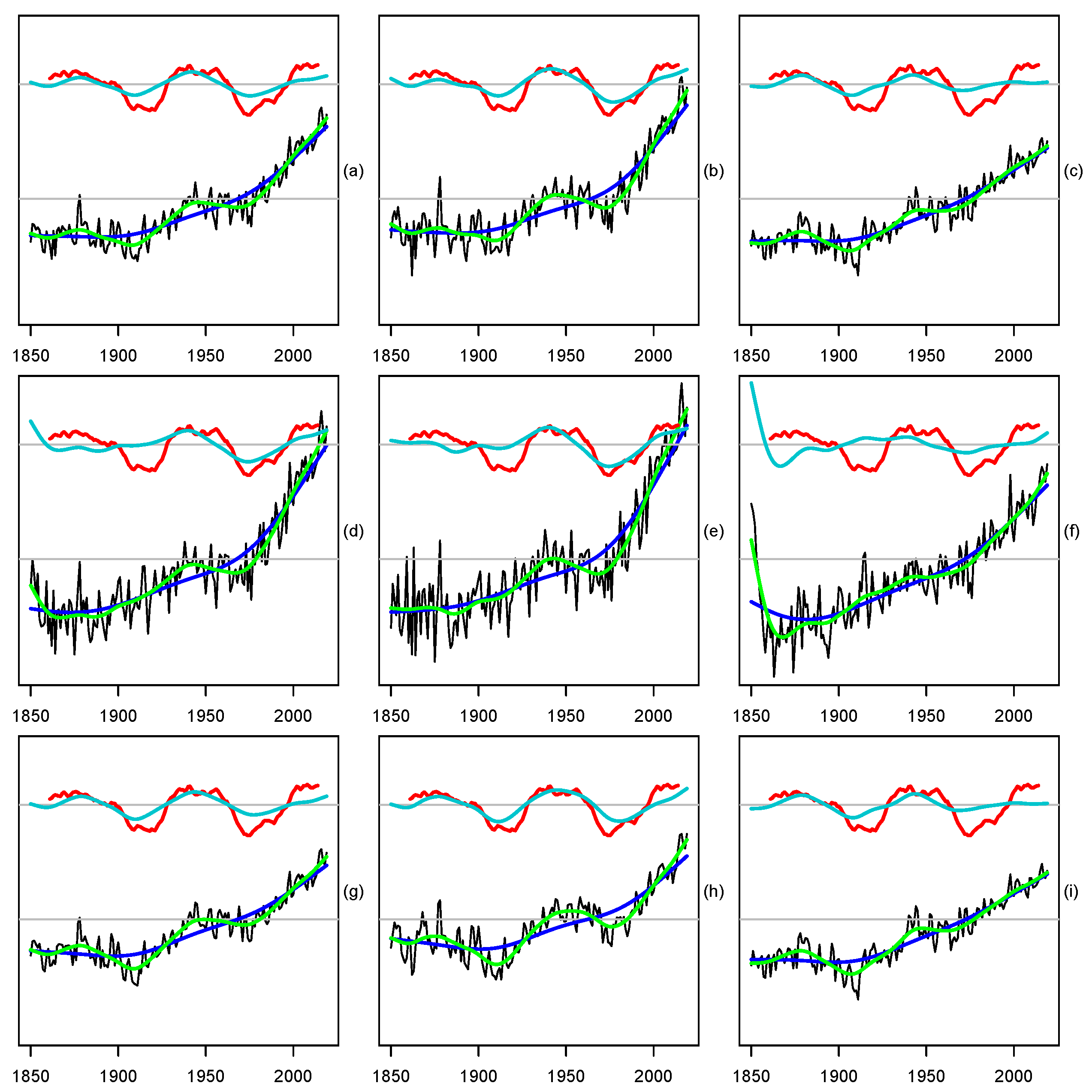
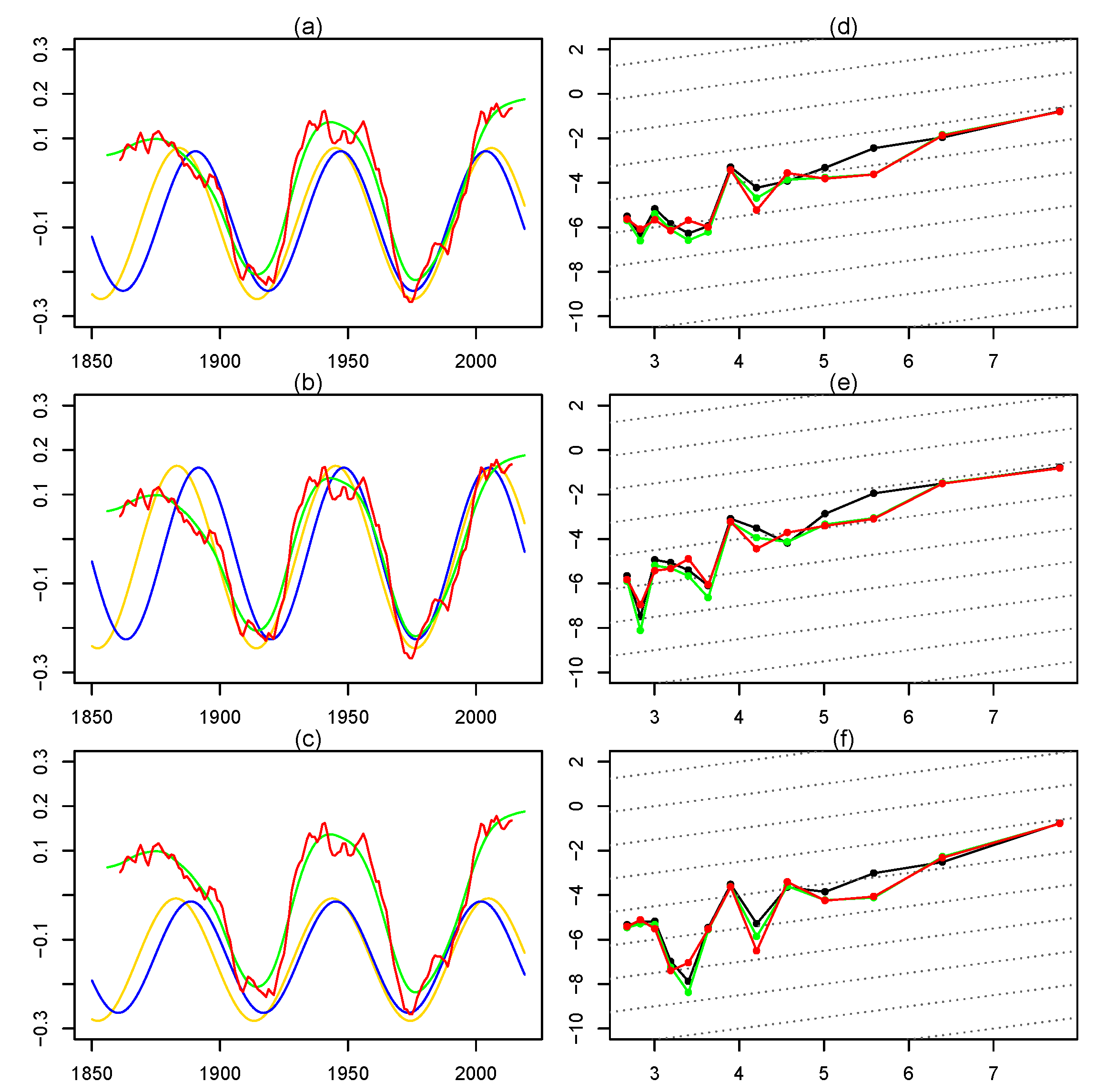
By definition, the AMO is closely related to the NH sea temperature series. In Figure 3h, this close relationship is illustrated graphically by applying the Hodrick—Prescott (HP) filter with a medium and a large smoothing parameter to the NH sea temperature series and comparing the difference with the smoothed AMO series. The similarity to the smoothed AMO series was still visible when the global sea temperature series (Figure 3g) or the corresponding combined sea and land temperature series (Figure 3b: NH, Figure 3a: global) are used instead. This meant that, in principle, an oscillation like the AMO could also have been defined on the basis of the global combined temperature series. However, in this case, we would be reluctant to filter out the whole oscillation because we would be aware that it is the sum of an unknown “periodic” component and random fluctuations with similar periods. This line of reasoning is corroborated by Figure 4d, which shows the log periodogram of the global temperature series after the removal of the AMO (by a regression on the smoothed AMO or on an estimate obtained by applying a HP-filter to the unsmoothed AMO), and the corresponding figures for the two hemispheric series (Figure 4e,f). While the third periodogram ordinate (from the right because the log periodogram was plotted against −1 times the log frequency) was well above the regression lines in Figure 2e, it was now substantially smaller, which indicates that the AMO removal has possibly gone too far. Noting that the AMO can be approximated very well by a sinusoid with a period of 61 years and still quite satisfactorily by a sinusoid with a period of years (see Figure 4a), which corresponds to the third Fourier frequency, we may alternatively account for the AMO in the frequency domain just by omitting the third periodogram ordinate.
For a robustness check of our earlier test results, we employed the test based on the statistic again, first after the removal of the AMO in the time domain by regressing the temperature on the smoothed AMO and second after the omission of the third periodogram ordinate. The fact that the first approach probably removed too much and the second approach too little is not the only possible cause for discrepancies in the results. There was also a difference in the sample sizes which was due to the fact that the AMO series were shorter. We therefore used the HadCRUT4 dataset only for the examination of the effect of the AMO-removal in the frequency domain. For the AMO-removal in the time domain, we used the shorter NH temperature series from the GISS dataset and, in addition, replaced the smoothed AMO series by the series obtained by applying the HP-filter with to the unsmoothed AMO. Table 2 shows that the test results obtained for the global temperature series hardly changed when the third Fourier frequency was omitted. Furthermore, comparing the last two columns of Table 2, which show the test results for the original and the AMO-detrended NH temperature series, respectively, we again found no noticeable differences, hence we concluded that the rejection of the null hypothesis of stationarity was not just due to the AMO.
4. Discussion
In this article, we have employed new frequency domain-methods for the investigation of global and hemispheric temperature series in order to obtain conclusive evidence of a long-term persistent change in the climate. Regardless whether there is a deterministic upward trend, a stochastic trend, or too strong serial correlation in the temperature series, there will always be a very steep increase in the spectral density in the neighborhood of frequency zero, which can be estimated or subjected to a formal statistical test. The advantage of this focus on a narrow frequency band is that no strong assumptions about the data generating process are required. The disadvantage is that the proof of a steep increase implies only that the temperature series are non-stationary but does not provide any details about the true nature of these series.
While establishing evidence of global warming in a statistically sound way is important in its own right, issues of more practical relevance must, of course, still be studied in a more concrete setting. For example, employing highly complex econometric models, Morana and Sbrana (2019) found that global warming (which is driven by radiative forcing) might directly enhance Atlantic hurricanes intensity/risk, which is inconsistent with the steady decline in the risk premia for catastrophe bonds since their introduction in the mid-1990s. Pretis (2020) showed that energy-balance models, which describe the change in temperatures as a function of incoming and outgoing radiation, can be mapped to cointegrated vector autoregressions, which allows the use of standard econometric techniques for the estimation of climate responses and the testing of their feedback.
Unfortunately, conventional tests of stationarity are based on asymptotic arguments and are therefore not really appropriate for temperature series, which are relatively short because there are too few data available from the period before 1850 (or even 1880 under more stringent criteria) for the estimation of global averages (for analyses of longer time series which are based on estimates rather than measurements, see, e.g., (Mills 2012; Davidson et al. 2016)). We have therefore employed a new small-sample test proposed by Mangat and Reschenhofer (2019), which is based on the comparison of the cumulative normalized periodogram in a narrow frequency band close to frequency zero with the cumulative distribution function of the standard uniform distribution. This test requires only that the standard distributional assumptions for the included periodogram ordinates hold approximately, which is plausible when the sample size is not too small. However, in contrast to conventional frequency-domain tests, the number of included frequencies do not have to be large too. The results obtained with this test after suitably transforming the temperature series and slightly modifying the null hypothesis are highly significant. These findings are corroborated by the estimates of the memory parameter obtained with various methods, which lie all in the region of non-stationarity.
However, even when the frequency band under consideration is very small, there is still the danger of distortions caused by low-frequency oscillations such as the AMO. Since the AMO mainly influences the northern hemisphere climate, we checked the robustness of our findings by testing the hypothesis of stationarity separately for the NH temperature series after the removal of the AMO. Regardless whether the AMO was removed in the time domain or in the frequency domain, the test results remained significant. We conclude that our empirical evidence of a persistent change in the surface temperature is genuine and not just due to a stationary phenomenon like the AMO.
Author Contributions
Both authors have contributed equally to all aspects of the work. They have both read and agreed to the published version of the manuscript.
Funding
This research received no external funding.
Acknowledgments
The authors gratefully acknowledge Open Access Funding by the University of Vienna and thank three anonymous reviewers for helpful comments and suggestions.
Conflicts of Interest
The authors declare no conflict of interest.
References
- Baiardi, Donatella, and Claudio Morana. 2020. Climate Change Awareness: Empirical Evidence for the European Union. University of Milan Bicocca Department of Economics, Management and Statistics Working Paper No. 426. January. Available online: https://ssrn.com/abstract=3513061 (accessed on 5 July 2020).
- Chang, Yoosoon, Robert K. Kaufmann, Chang Sik Kim, J. Isaac Miller, Joon Y. Park, and Sungkeun Park. 2020. Evaluating trends in time series of distributions: A spatial fingerprint of human effects on climate. Journal of Econometrics 214: 274–94. [Google Scholar] [CrossRef]
- Davidson, James E.H., David B. Stephenson, and Alemtsehai A. Turasie. 2016. Time series modeling of paleoclimate data. Environmetrics 27: 55–65. [Google Scholar] [CrossRef]
- Delworth, Thomas L., and Michael E. Mann. 2000. Observed and simulated multidecadal variability in the northern hemisphere. Climate Dynamics 16: 661–76. [Google Scholar] [CrossRef] [Green Version]
- Dickey, David A., and Wayne A. Fuller. 1979. Distribution of the estimators for autoregressive time series with a unit root. Journal of the American Statistical Association 74: 427–31. [Google Scholar]
- Dickey, David A., and Wayne A. Fuller. 1981. Likelihood ratio statistics for autoregressive time series with a unit root. Econometrica: Journal of the Econometric Society 49: 1057–72. [Google Scholar] [CrossRef]
- Estrada, Francisco, Luis Filipe Martins, and Pierre Perron. 2017. Characterizing and attributing the warming trend in sea and land surface temperatures. Atmósfera 30: 163–87. [Google Scholar] [CrossRef] [Green Version]
- Estrada, Francisco, and Pierre Perron. 2019. Breaks, trends and the attribution of climate change: A time-series analysis. Economía 42: 1–31. [Google Scholar] [CrossRef] [Green Version]
- Estrada, Francisco, Pierre Perron, and Benjamín Martínez-López. 2013. Statistically derived contributions of diverse human influences to twentieth-century temperature changes. Nature Geoscience 6: 1050–55. [Google Scholar] [CrossRef] [Green Version]
- Fomby, Thomas B., and Timothy J. Vogelsang. 2002. The application of size-robust trend statistics to global-warming temperature series. Journal of Climate 15: 117–23. [Google Scholar] [CrossRef] [Green Version]
- Gay-Garcia, Carlos, Francisco Estrada, and Armando Sánchez. 2009. Global and hemispheric temperatures revisited. Climatic Change 94: 333–49. [Google Scholar] [CrossRef]
- Geweke, John, and Susan Porter-Hudak. 1983. The estimation and application of long memory time series models. Journal of Time Series Analysis 4: 221–38. [Google Scholar] [CrossRef]
- Granger, Clive W.J., and Roselyne Joyeux. 1980. An introduction to long-memory time series models and fractional differencing. Journal of Time Series Analysis 1: 15–29. [Google Scholar] [CrossRef]
- Grenander, Ulf, and Murray Rosenblatt. 1957. Statistical Analysis of Stationary Time Series. New York: John Wiley and Sons. [Google Scholar]
- Harvey, David I., Stephen J. Leybourne, and A.M. Robert Taylor. 2013. Testing for unit roots in the possible presence of multiple trend breaks using minimum dickey–fuller statistics. Journal of Econometrics 177: 265–84. [Google Scholar] [CrossRef]
- Hassler, Uwe. 1993. Regression of spectral estimators with fractionally integrated time series. Journal of Time Series Analysis 14: 369–80. [Google Scholar] [CrossRef]
- Hosking, Jonathan R. M. 1981. Fractional differencing. Biometrika 68: 165–76. [Google Scholar] [CrossRef]
- Hurvich, Clifford M., Rohit Deo, and Julia Brodsky. 1998. The mean squared error of geweke and porter-hudak’s estimator of the memory parameter of a long-memory time series. Journal of Time Series Analysis 19: 19–46. [Google Scholar] [CrossRef]
- Jones, Philip. D., Dave H. Lister, Timothy J. Osborn, Colin Harpham, Melissa Salmon, and Colin P. Morice. 2012. Hemispheric and large-scale land-surface air temperature variations: An extensive revision and an update to 2010. Journal of Geophysical Research: Atmospheres 117. [Google Scholar] [CrossRef] [Green Version]
- Kaufmann, Robert K., Heikki Kauppi, and James H. Stock. 2006. Emissions, concentrations, & temperature: A time series analysis. Climatic Change 77: 249–78. [Google Scholar]
- Kaufmann, Robert K., Heikki Kauppi, and James H. Stock. 2010. Does temperature contain a stochastic trend? evaluating conflicting statistical results. Climatic Change 101: 395–405. [Google Scholar] [CrossRef]
- Kaufmann, Robert K., and David I. Stern. 2002. Cointegration analysis of hemispheric temperature relations. Journal of Geophysical Research: Atmospheres 107: ACL-8. [Google Scholar] [CrossRef] [Green Version]
- Kennedy, John J., Nick A. Rayner, Robert O. Smith, David E. Parker, and Michael Saunby. 2011. Reassessing biases and other uncertainties in sea surface temperature observations measured in situ since 1850: 2. Biases and homogenization. Journal of Geophysical Research: Atmospheres 116. [Google Scholar] [CrossRef]
- Künsch, Hans Rudolph. 1986. Discrimination between monotonic trends and long-range dependence. Journal of applied Probability 23: 1025–30. [Google Scholar] [CrossRef]
- Künsch, Hans Rudolph. 1987. Statistical aspects of self-similar processes. In Proceedings of the First World Congress of the Bernoulli Society. Tashkent: VNU Science Press, pp. 67–74. [Google Scholar]
- Kwiatkowski, Denis, Peter C. B. Phillips, Peter Schmidt, and Yongcheol Shin. 1992. Testing the null hypothesis of stationarity against the alternative of a unit root. Journal of Econometrics 54: 159–78. [Google Scholar] [CrossRef]
- Lai, Kon S., and Mann Yoon. 2018. Nonlinear trend stationarity in global and hemispheric temperatures. Applied Economics Letters 25: 15–18. [Google Scholar] [CrossRef]
- Lee, Tien Ming, Ezra M. Markowitz, Peter D. Howe, Chia-Ying Ko, and Anthony A. Leiserowitz. 2015. Predictors of public climate change awareness and risk perception around the world. Nature Climate Change 5: 1014–20. [Google Scholar] [CrossRef]
- Lenssen, Nathan J. L., Gavin A. Schmidt, James E. Hansen, Matthew J. Menne, Avraham Persin, Reto Ruedy, and Daniel Zyss. 2019. Improvements in the gistemp uncertainty model. Journal of Geophysical Research: Atmospheres 124: 6307–26. [Google Scholar] [CrossRef]
- Mangat, Manveer Kaur, and Erhard Reschenhofer. 2019. Testing for long-range dependence in financial time series. Central European Journal of Economic Modelling and Econometrics (CEJEME) 11: 93–106. [Google Scholar]
- Mills, Terence C. 2012. Semi-parametric modelling of temperature records. Journal of Applied Statistics 39: 361–83. [Google Scholar] [CrossRef]
- Morana, Claudio, and Giacomo Sbrana. 2019. Climate change implications for the catastrophe bonds market: An empirical analysis. Economic Modelling 81: 274–94. [Google Scholar] [CrossRef]
- Morice, Colin P., John J. Kennedy, Nick A. Rayner, and Phil D. Jones. 2012. Quantifying uncertainties in global and regional temperature change using an ensemble of observational estimates: The hadcrut4 data set. Journal of Geophysical Research: Atmospheres 117. [Google Scholar] [CrossRef]
- Ng, Serena, and Pierre Perron. 2001. Lag length selection and the construction of unit root tests with good size and power. Econometrica 69: 1519–54. [Google Scholar] [CrossRef] [Green Version]
- Peiris, M. Shelton, and J. R. Court. 1993. A note on the estimation of degree of differencing in long memory time series analysis. Probability and Mathematical Statistics 14: 223–229. [Google Scholar]
- Perron, Pierre, and Zhongjun Qu. 2007. A simple modification to improve the finite sample properties of ng and perron’s unit root tests. Economics Letters 94: 12–19. [Google Scholar] [CrossRef]
- Perron, Pierre, and Gabriel Rodríguez. 2003. Gls detrending, efficient unit root tests and structural change. Journal of Econometrics 115: 1–27. [Google Scholar] [CrossRef] [Green Version]
- Perron, Pierre, and Tomoyoshi Yabu. 2009. Testing for shifts in trend with an integrated or stationary noise component. Journal of Business & Economic Statistics 27: 369–96. [Google Scholar]
- Phillips, Peter C. B., and Pierre Perron. 1988. Testing for a unit root in time series regression. Biometrika 75: 335–46. [Google Scholar] [CrossRef]
- Poortinga, Wouter, Stephen Fisher, Gisela Bohm, Linda Steg, Lorraine Whitmarsh, and Charles Ogunbode. 2018. European Attitudes to Climate Change and Energy: Topline Results from Round 8 of the European Social Survey. ESS Topline Results Series; London: University of London. [Google Scholar]
- Pötscher, Benedikt M. 2002. Lower risk bounds and properties of confidence sets for ill-posed estimation problems with applications to spectral density and persistence estimation, unit roots, and estimation of long memory parameters. Econometrica 70: 1035–65. [Google Scholar] [CrossRef]
- Pretis, Felix. 2020. Econometric modelling of climate systems: The equivalence of energy balance models and cointegrated vector autoregressions. Journal of Econometrics 214: 256–73. [Google Scholar] [CrossRef]
- Reisen, Valderio A. 1994. Estimation of the fractional difference parameter in the arima (p, d, q) model using the smoothed periodogram. Journal of Time Series Analysis 15: 335–50. [Google Scholar] [CrossRef]
- Reschenhofer, Erhard. 2013. Robust testing for stationarity of global surface temperature. Journal of Applied Statistics 40: 1349–61. [Google Scholar] [CrossRef]
- Reschenhofer, Erhard, and Manveer Kaur Mangat. 2020. Detecting long-range dependence with truncated ratios of periodogram ordinates. Communications in Statistics—Theory and Methods, 1–16. [Google Scholar] [CrossRef] [Green Version]
- Reschenhofer, Erhard, Manveer Kaur Mangat, and Thomas Stark. 2020. Improved estimation of the memory parameter. Theoretical Economics Letters 10: 47–68. [Google Scholar] [CrossRef] [Green Version]
- Robinson, Peter M. 1995. Gaussian semiparametric estimation of long range dependence. The Annals of Statistics 23: 1630–61. [Google Scholar] [CrossRef]
- Schmidt, Peter, and Peter C. B. Phillips. 1992. Lm tests for a unit root in the presence of deterministic trends. Oxford Bulletin of Economics and Statistics 54: 257–87. [Google Scholar] [CrossRef]
- Stern, David I., and Robert K. Kaufmann. 1999. Econometric analysis of global climate change. Environmental Modelling & Software 14: 597–605. [Google Scholar]
- Vogelsang, Timothy J. 1998. Trend function hypothesis testing in the presence of serial correlation. Econometrica 66: 123–48. [Google Scholar] [CrossRef]
Figure 1.
Realizations of fractional white noise with different values of the memory parameter (a,d,f: , b,e,h: , c,f,i: ) and different sample sizes (a–c: , d–f: , g–i: ) but with the same standard normal innovations.
Figure 1.
Realizations of fractional white noise with different values of the memory parameter (a,d,f: , b,e,h: , c,f,i: ) and different sample sizes (a–c: , d–f: , g–i: ) but with the same standard normal innovations.

Figure 2.
Global temperature: (a,c,e); Differenced global temperature (b,d,f); (a,b): Plot of time series; (c,d): Periodogram of time series; (e,f): Log periodogram ordinates plotted against along with various estimates of d (: red, : blue, : green, : gold) based on Fourier frequencies and parallel lines (gray, dotted) with slope 0.5, which represent the boundary of the region of non-stationarity (the slope is −0.5 in the case of the differenced series).

Figure 3.
Applying the Hodrick–Prescott filter with two different degrees of smoothing (blue: green: 100,000) to different temperature series (from the HadCRUT4, CRUTEM4, HadSST3 datasets) and comparing the difference (turquoise) with the smoothed AMO series (red). (a–c): combined land and sea, (d–f): land, (g–i): sea, (a,d,g): global, (b,e,h): northern hemisphere, (c,f,i): southern hemisphere.

Figure 4.
In the first column, sinusoids with periods 61 (gold) and (blue) are fitted to (a) global, (b) northern hemisphere, (c) southern hemisphere temperature series 1850–2019 of length and plotted together with two different AMO series (smoothed AMO series 1861–2014: red, HP filter with applied to unsmoothed AMO series 1856–2019: green). In the second column, the log periodogram ordinates , , obtained from the original temperature series (black) and two versions of AMO-detrended temperature series (smoothed AMO: red, HP-filter: green) are plotted against for different regions ((d): global, (e): northern hemisphere, (f): southern hemisphere). The parallel lines (gray, dotted) with slope 0.5 represent the boundary of the non-stationarity region.


Table 1.
Estimates of d obtained by applying the estimators , , , , and based on the first K Fourier frequencies to the annual global surface air temperature series (1850–2019).
Table 1.
Estimates of d obtained by applying the estimators , , , , and based on the first K Fourier frequencies to the annual global surface air temperature series (1850–2019).
| K | ||||||
|---|---|---|---|---|---|---|
| 6 | 0.90 | 0.95 | 1.14 | 0.94 | 0.90 | 0.93 |
| 7 | 0.90 | 0.94 | 1.15 | 0.97 | 0.90 | 0.92 |
| 8 | 1.48 | 1.98 | 1.11 | 0.97 | 1.06 | 1.16 |
| 9 | 1.30 | 1.57 | 1.10 | 0.97 | 0.96 | 0.90 |
| 10 | 1.17 | 1.32 | 1.04 | 0.95 | 0.91 | 0.87 |
| 11 | 1.14 | 1.25 | 1.01 | 0.94 | 0.94 | 0.92 |
| 12 | 1.12 | 1.20 | 0.98 | 0.93 | 0.97 | 0.96 |
| 13 | 1.12 | 1.19 | 0.98 | 0.93 | 1.00 | 1.00 |
| 14 | 1.10 | 1.16 | 0.96 | 0.91 | 1.02 | 1.03 |
| 15 | 1.02 | 1.04 | 0.93 | 0.90 | 0.93 | 0.86 |
Table 2.
Values of the test statistic obtained for the annual global and hemispheric (NH: northern hemisphere, SH: southern hemisphere) temperature series when the lowest K Fourier frequencies (possibly excl. the third) are used to test the null hypotheses (if ) and (if ). Significance at the , , and level is indicated by (*), (**), and (***), respectively.
| K | Global | Excl. 3rd | NH | SH | NH (GISS) | AMO-detr. (HP) | |
|---|---|---|---|---|---|---|---|
| 0.4 | 8 | 0.446 ** | 0.486 ** | 0.444 ** | 0.444 ** | 0.46 ** | 0.444 ** |
| 10 | 0.437 ** | 0.447 ** | 0.447 ** | 0.42 ** | 0.46 ** | 0.447 ** | |
| 12 | 0.456 *** | 0.448 ** | 0.473 *** | 0.427 ** | 0.418 ** | 0.473 *** | |
| 14 | 0.468 *** | 0.459 *** | 0.475 *** | 0.444 *** | 0.412 *** | 0.475 *** | |
| 0.49 | 8 | 0.404 * | 0.425 * | 0.405 * | 0.398 * | 0.407 * | 0.405 * |
| 10 | 0.382 * | 0.375 * | 0.397 ** | 0.358 * | 0.403 ** | 0.397 ** | |
| 12 | 0.396 ** | 0.376 ** | 0.42 ** | 0.36 ** | 0.353 ** | 0.42 ** | |
| 14 | 0.41 *** | 0.387 ** | 0.418 *** | 0.375 ** | 0.345 ** | 0.418 *** | |
| 0.5 | 8 | 0.399 * | 0.418 * | 0.4 * | 0.393 * | 0.401 * | 0.4 * |
| 10 | 0.376 * | 0.367 * | 0.391 ** | 0.351 * | 0.397 ** | 0.391 ** | |
| 12 | 0.39 ** | 0.369 * | 0.414 ** | 0.352 * | 0.346 * | 0.414 ** | |
| 14 | 0.403 ** | 0.379 ** | 0.412 *** | 0.367 ** | 0.338 ** | 0.412 *** | |
| −0.4 | 8 | 0.468 ** | 0.494 ** | 0.525 ** | 0.292 | 0.528 ** | 0.525 ** |
| 10 | 0.444 ** | 0.47 ** | 0.504 *** | 0.268 | 0.5 *** | 0.504 *** | |
| 12 | 0.414 ** | 0.439 ** | 0.469 *** | 0.25 | 0.442 *** | 0.469 *** | |
| 14 | 0.404 *** | 0.428 *** | 0.455 *** | 0.23 | 0.419 *** | 0.455 *** |
Table 3.
Rejection rates for the true null hypothesis H at the and levels of significance obtained by applying the one-sided test based on with to 5000 realizations () of a Gaussian fractionally integrated ARMA (ARFIMA) process with memory parameter and AR-parameter .
Table 3.
Rejection rates for the true null hypothesis H at the and levels of significance obtained by applying the one-sided test based on with to 5000 realizations () of a Gaussian fractionally integrated ARMA (ARFIMA) process with memory parameter and AR-parameter .
| 1% | 5% | ||||||||
|---|---|---|---|---|---|---|---|---|---|
| 0.4 | −0.1 | 0.011 | 0.011 | 0.012 | 0.010 | 0.052 | 0.054 | 0.058 | 0.052 |
| 0 | 0.010 | 0.012 | 0.010 | 0.010 | 0.059 | 0.049 | 0.055 | 0.062 | |
| 0.1 | 0.011 | 0.012 | 0.011 | 0.012 | 0.056 | 0.060 | 0.059 | 0.050 | |
| 0.49 | −0.1 | 0.014 | 0.012 | 0.011 | 0.012 | 0.059 | 0.059 | 0.056 | 0.064 |
| 0 | 0.012 | 0.012 | 0.012 | 0.013 | 0.053 | 0.061 | 0.058 | 0.059 | |
| 0.1 | 0.012 | 0.014 | 0.015 | 0.014 | 0.062 | 0.059 | 0.060 | 0.064 | |
| 0.5 | −0.1 | 0.010 | 0.013 | 0.013 | 0.012 | 0.054 | 0.057 | 0.058 | 0.056 |
| 0 | 0.013 | 0.016 | 0.011 | 0.012 | 0.062 | 0.059 | 0.059 | 0.060 | |
| 0.1 | 0.009 | 0.013 | 0.010 | 0.013 | 0.059 | 0.063 | 0.065 | 0.058 | |
| −0.4 | −0.1 | 0.017 | 0.014 | 0.015 | 0.015 | 0.069 | 0.066 | 0.072 | 0.071 |
| 0 | 0.016 | 0.017 | 0.014 | 0.019 | 0.070 | 0.070 | 0.065 | 0.067 | |
| 0.1 | 0.014 | 0.017 | 0.017 | 0.015 | 0.073 | 0.069 | 0.065 | 0.068 | |
Table 4.
Rejection rates for the false hypothesis at the level of significance obtained by applying the one-sided test based on with to 5000 realizations () of a Gaussian ARFIMA process with memory parameter and AR-parameter .
Table 4.
Rejection rates for the false hypothesis at the level of significance obtained by applying the one-sided test based on with to 5000 realizations () of a Gaussian ARFIMA process with memory parameter and AR-parameter .
| 0.4 | −0.1 | 0.363 | 0.45 | 0.545 | 0.619 | 0.649 | 0.777 | 0.854 | 0.914 | 0.797 | 0.903 | 0.963 | 0.983 |
| 0 | 0.381 | 0.459 | 0.555 | 0.623 | 0.663 | 0.781 | 0.877 | 0.915 | 0.797 | 0.897 | 0.960 | 0.985 | |
| 0.1 | 0.372 | 0.476 | 0.551 | 0.63 | 0.653 | 0.785 | 0.864 | 0.915 | 0.792 | 0.906 | 0.956 | 0.985 | |
| 0.49 | −0.1 | 0.259 | 0.321 | 0.393 | 0.439 | 0.527 | 0.659 | 0.762 | 0.837 | 0.658 | 0.812 | 0.901 | 0.949 |
| 0 | 0.259 | 0.331 | 0.384 | 0.445 | 0.526 | 0.668 | 0.754 | 0.84 | 0.663 | 0.805 | 0.903 | 0.947 | |
| 0.1 | 0.271 | 0.321 | 0.389 | 0.446 | 0.547 | 0.67 | 0.774 | 0.839 | 0.663 | 0.818 | 0.900 | 0.946 | |
| 0.5 | −0.1 | 0.257 | 0.314 | 0.372 | 0.428 | 0.517 | 0.643 | 0.748 | 0.817 | 0.657 | 0.795 | 0.895 | 0.942 |
| 0 | 0.248 | 0.299 | 0.374 | 0.413 | 0.517 | 0.659 | 0.745 | 0.817 | 0.656 | 0.792 | 0.891 | 0.948 | |
| 0.1 | 0.252 | 0.326 | 0.379 | 0.431 | 0.518 | 0.64 | 0.755 | 0.828 | 0.651 | 0.808 | 0.883 | 0.943 | |
| −0.4 | −0.1 | 0.142 | 0.171 | 0.194 | 0.211 | 0.394 | 0.498 | 0.578 | 0.655 | 0.697 | 0.809 | 0.891 | 0.937 |
| 0 | 0.140 | 0.181 | 0.195 | 0.221 | 0.392 | 0.493 | 0.591 | 0.665 | 0.704 | 0.810 | 0.892 | 0.939 | |
| 0.1 | 0.152 | 0.170 | 0.202 | 0.224 | 0.406 | 0.506 | 0.588 | 0.669 | 0.692 | 0.813 | 0.894 | 0.943 | |
© 2020 by the authors. Licensee MDPI, Basel, Switzerland. This article is an open access article distributed under the terms and conditions of the Creative Commons Attribution (CC BY) license (http://creativecommons.org/licenses/by/4.0/).
Share and Cite
MDPI and ACS Style
Mangat, M.K.; Reschenhofer, E. Frequency-Domain Evidence for Climate Change. Econometrics 2020, 8, 28. https://0-doi-org.brum.beds.ac.uk/10.3390/econometrics8030028
AMA Style
Mangat MK, Reschenhofer E. Frequency-Domain Evidence for Climate Change. Econometrics. 2020; 8(3):28. https://0-doi-org.brum.beds.ac.uk/10.3390/econometrics8030028
Chicago/Turabian StyleMangat, Manveer Kaur, and Erhard Reschenhofer. 2020. "Frequency-Domain Evidence for Climate Change" Econometrics 8, no. 3: 28. https://0-doi-org.brum.beds.ac.uk/10.3390/econometrics8030028
Note that from the first issue of 2016, this journal uses article numbers instead of page numbers. See further details here.