The Discovery of Long-Run Causal Order: A Preliminary Investigation †

1
Department of Economics, Duke University, Durham, NC 27708, USA
2
Department of Philosophy, Duke University, Durham, NC 27708, USA
†
This paper arises out of a joint project with Søren Johansen, Katarina Juselius: they have been inspiring teachers, candid critics, and true friends. I am grateful for earlier collaboration with Morten Nyboe Tabor and for the skeptical, but invaluable, comments of the guest editors for the special issue, Paolo Paruolo and Rocco Mosconi, and three anonymous referees. A very early version of the paper was presented at the Econometrics Conference, Programme for Economic Modelling, University of Oxford, 1–2 September 2014. I thank the participants for valuable comments.
Econometrics 2020, 8(3), 31; https://0-doi-org.brum.beds.ac.uk/10.3390/econometrics8030031
Submission received: 10 May 2018
/
Revised: 16 July 2020
/
Accepted: 23 July 2020
/
Published: 3 August 2020
(This article belongs to the Special Issue Celebrated Econometricians: Katarina Juselius and Søren Johansen)
Abstract
:The relation between causal structure and cointegration and long-run weak exogeneity is explored using some ideas drawn from the literature on graphical causal modeling. It is assumed that the fundamental source of trending behavior is transmitted from exogenous (and typically latent) trending variables to a set of causally ordered variables that would not themselves display nonstationary behavior if the nonstationary exogenous causes were absent. The possibility of inferring the long-run causal structure among a set of time-series variables from an exhaustive examination of weak exogeneity in irreducibly cointegrated subsets of variables is explored and illustrated.
Keywords:
graphical causal modeling; causal search; cointegrated vector autoregression (CVAR); weak exogeneity; irreducible cointegrating relationsJEL Classification:
C32; C51; C18In the long run, we are all dead.John Maynard KeynesIn the long run, we are simply in another short run.variously attributedContrary to Keynes’ famous dictum in the long run we are all dead,the long run is with us every day of our livesWalt Rostow
1. The Problem of Causal Order in the CVAR
Katarina Juselius and Søren Johansen’s most famous contributions to econometrics, studied in detail and applied in his monograph (Johansen 1995) and in her textbook (Juselius 2006), and, jointly and singly, in a large number of journal articles, concern the cointegrated vector autoregression (CVAR). The CVAR focuses special attention on the nonstationary components and the long-run properties of the time series. The questions we address in this paper are how the long-run properties of the CVAR can be given a structural interpretation and how that interpretation might support inference of the long-run causal structure from the observable characteristics of the nonstationary data.
There are two significant traditions in time-series econometrics.1 The Cowles Commission in the 1940s and 1950s pioneered structural econometrics that conceived of the econometric problem as one of articulating and measuring economic mechanisms (Koopmans 1950; Hood and Koopmans 1953; see Morgan 1990 for a history). The articulation of mechanisms was generally referred to as the “identification problem.” The major resource for securing identification was a priori economic theory. Early on, structural and causal articulation were regarded as synonymous, although subsequently causal language fell from favor (Hoover 2004). In his contribution to the 1953 Cowles volume, Herbert Simon (1953) drew on the language of experiments (actual or metaphorical) to suggest that an identified system of dynamic equations provided a map of the space of interventions in the economy.2 Simon demonstrated an isomorphism between a structurally identified model and a causally well-ordered model in a system with no stochastic variables.
A second econometric tradition, grounded more in time-series statistics, focused on process rather than structure (e.g., see Wold 1960; Granger 1969). Granger defined causality in terms of incremental predictability. Sims (1972) introduced Granger causality into empirical macroeconomics. Frequently thereafter, an equivocation between Granger’s notion of causality and structural notions became commonplace. Granger himself was aware that Granger causality did not address the questions of control and counterfactual policy analysis that motivated structural understandings of causality, such as those of Simon and the Cowles Commission (Granger 1969, 1995; also White and Lu 2010, p. 194). While both the structural and the process approaches to econometrics have a concept of causation, those concepts are distinct. They may, nonetheless, be mutually informative. White and Lu (2010) and White and Pettenuzzo (2014), for instance, analyze the conditions under which Granger causality can provide information relevant to assessing structural causality (see also Hoover 2001, pp. 150–55).
The vector autoregression (VAR) arises out of the process tradition. Building on earlier criticisms of Liu (1960) and others, Christopher Sims (1980) introduced the VAR into macroeconometrics as part of a critical response to the Cowles Commission approach. Christopher Sims (1980, p. 1), attacked the structural interpretation of econometric models for using “incredible” identifying restrictions. Initially, he offered the VAR—a system of reduced-form equations in which all variables are endogenous—as a workable alternative to identified structural models.
There is a tendency to treat process accounts of causality as essentially atheoretical and data driven and to treat structural accounts as necessarily relying on a priori theory. These connections are more accidents of the history of econometrics than essential. In the case of the VAR, it rapidly became clear that reduced-form VARs were inadequate to the needs of counterfactual policy analysis—perhaps the most important use of macroeconometric models (Cooley and LeRoy 1985; Sims 1982, 1986). The structural VAR (SVAR), which imposes a causal order on the contemporaneous relationships among the endogenous variables, was seen to provide the minimum restrictions needed to identify independent shocks, which were taken to be the drivers of a dynamic system, and policy analysis was largely reduced to working out the impulse responses to those shocks (see Duarte and Hoover 2012; Hoover and Jordá 2001).
While the problem that had motivated Sims in the first place, the incredibility of the identifying restrictions, had been minimized in the SVAR, it was not eliminated; and the question, how we are to know the correct contemporaneous causal order, remains an open one. In truth, economic theory rarely provides a clear or decisive answer. In practice in most, though not all cases, SVARs were identified by assuming certain triangular causal orderings of the contemporaneous variables. Since all such causal orders are just identified, they have the same likelihood function, and, thus, there is no empirical basis for choosing among them, so long as “empirical” is restricted to likelihood information. At this point, SVAR practitioners typically claim that it is necessary to invoke prior information from economic theory or practical institutional knowledge or common sense to pick among the equivalent causal orders. In fact, however, empirical evidence can be brought to bear on the choice. When the underlying data-generating processes (DGPs) are casually ordered in such a way that an empirically valid model of it would be over-identified, information about conditional dependence and independence among the variables in some cases will provide information that can be used to distinguish among possible causal orders. This approach has been developed with great sophistication (mainly for non-time-series data) in the so-called graphical-causal-modeling or Bayes-net literature (Spirtes et al. 2000; Pearl 2009).3 Swanson and Granger (1997) first applied a simple graphical causal search algorithm to the problem of determining the contemporaneous causal structure of an SVAR. Subsequently, more sophisticated algorithms have been applied and shown to be effective in a wide range of circumstances (Demiralp and Hoover 2003; Demiralp et al. 2008; and references therein).
Meanwhile, time-series econometrics discovered the importance of nonstationary processes and the concept of cointegration (Engle and Granger 1987). In light of these developments, the SVAR was reformulated into the CVAR. Throughout the paper, we will consider cases in which we, in fact, know the true DGP, but observe only some part of it. To be clear, our operating assumption is that a complex data-generating process governs the behavior of the economy; and the aim of structural causal modeling is to uncover a (partial) representation of the true DGP that is adequate to pragmatically required levels of detail and precision to support inter alia prediction and counterfactual analysis.4 A key question will be how much information about the DGP can be recovered from the observables.
Our interest is in long-run identification; so, we will restrict our attention to CVARs, taken to be a reduced form of a part of the economy’s unobserved DGP, of the form:
where X = [x1, x2, … xp]′ is a vector of variables integrated of degree one (notated I(1)), Π is a p × p matrices of parameters; E = [ε1, ε2, … εp]′ is p-element vector of normal residuals distributed Et ~ N(0, Ω); and t subscripts indicate time. The residuals contain both unobserved causes, which we shall call “shocks,” and various sorts of error. The matrix Ω is assumed to be diagonal. This assumption could be justified by economic theory or could result from orthogonalizing the residuals by multiplying through by a matrix that reflects the appropriate contemporaneous causal ordering in the manner that Choleski matrices are frequently used in the SVAR literature, a transformation that would affect the interpretation of the Xt’s.
If the variables in X are cointegrated (i.e., if a linear combination of nonstationary variables is itself stationary), then Π has reduced rank (r) and may be written as Π = αβ′, where α and β are p × r matrices. Such a CVAR is said to have r cointegrating relations and q = p−r common trends. The rows of β′ contain the cointegrating vectors; while the α matrix contains adjustment parameters. In general, the αβ′ decomposition in not unique, since α and β may take different values, so long as Π = αβ′ and still remain consistent with the observations modeled in Equation (1) (Johansen 1995, p. 71; Juselius 2006, p. 216). Most of the focus in identifying the CVAR has been placed on identifying the cointegrating vectors of the β′ on the basis of prior economic theory.
The goal of this paper is to provide a coherent account of the causal order of a CVAR and to make some preliminary suggestions about how the methods of graphical causal search in conjunction with cointegration analysis could aid in the empirical discovery of its long run, as they have already aided in the discovery of the contemporaneous causal structure.
2. Graph-Theoretic Causal Order
Where other investigators have mainly focused on the cointegrating relationships encapsulated in β′, we shift the focus to the closely related question of how trends are transmitted among the variables. Ours will be a preliminary investigation and will be restricted to cases in which all variables are I(1) and DGPs that can be adequately represented in a structural model that can be understood as a causally ordered consistent with a directed acyclical graph.
2.1. Graphs and Causal Structure
Several econometricians have given structural accounts of long-run behavior in the CVAR. They have focused mainly on the use of theory to provide the necessary identification (Davidson and Hall 1991; Pesaran and Shin 2002; Pesaran and Smith 1998; Pagan and Pesaran 2008). In contrast to economists’ frequent reliance on a priori theory, in the case of stationary data, considerable headway has been made (mostly, but not entirely, outside of economics) in developing graphical causal search algorithms that can narrow the class of admissible identifications—sometimes to a unique scheme (Spirtes et al. 2000; Pearl 2009). As a preliminary to examining how some of these ideas might be extended to the nonstationary case, it will be helpful to review selectively some aspects of graphical causal analysis.
In Simon’s (1953) account, a structural model is a system of equations representing mechanisms in the world.5 Although the account can be generalized considerably (see Hoover 1990; 2001, chp. 3), it will do for our purposes to restrict our attention to linear equations and to treat each equation as the representation of the causal mechanism determining its left-hand-side variable (the effect) in terms of right-hand-side variables (the direct causes). The coefficients on the right-hand-side variables are taken to define the space of interventions in the causal model. Thus, an intervention, for example, to a policy rule might change the numerical value of one of the coefficients in the equation representing the rule. In a well-defined structure, the coefficients could be intervened upon independently of each other.
We analyze a restricted version of the structural approach to causality, in that it does not deal with nonlinearities, such as cross-equation restrictions, that might arise in economic optimization problems or from systemic restrictions, such as may be generated under rational expectations. In part this is a pragmatic choice to deal with the easier case first; in part, it is to maintain tighter contact with the existing graph-theoretic causal search literature; and, in part, it arises from a yet-untested conjecture that considerable empirical progress can be made with respect to long-run cause in a simple framework. The structural approach can nonetheless be further generalized; see, for example, (Hoover 1990, appendix; 2001, especially chp. 3) and White and Chalak (2009).
Graph-theoretic causal analysis represents structural systems of equations as a directed graph. The variables form the nodes or vertices of the graph, and edges connect pairs of vertices. Edges come in several forms, but we will use only one—the single-headed arrow “→”, which means “directly causes”. Direct causes are also referred to as the parents of the effect or child. We restrict ourselves to directed acylical graphs (DAGs), which are adequate to the typical CVARs found in the macroeconomics literature. Graphical causal modeling is not, however, restricted to DAGs: the literature has also addressed cyclical graphs (for example, graphs in which A causes B, B causes C, and C causes A) and simultaneous graphs (a particularly tight form of cyclicality in which A causes B and B causes A) (see Richardson 1996; Phiromswad and Hoover 2013, and the references therein).
2.2. Graphs and Conditional Independence
The key idea in graph-theoretic accounts of causal structure is the mapping between the causal graph and the probability distribution described of the true DGP and its reduced form. The mapping is based on Reichenbach’s (1956, p. 156) Principle of the Common Cause: if any two variables, A and B, are probabilistically dependent, then either A causes B (A → B) or B causes A (A ← B) or they have a common cause (A ← C → B). Essentially, the idea behind the principle is that correlations may not be causation, but correlations nevertheless must have a causal explanation. The Principle of the Common Cause is generalized as the “causal Markov condition” (Spirtes et al. 2000, p. 29; see also Pearl 2009, p. 30).
Without going into detail, the graph encodes certain facts of (conditional) probabilistic dependence and independence among the variables. If the data were, in fact, generated by a system of equations corresponding to the graph—as they would be, for example, in a simulation—then the joint probability distribution for those variables would embody the encoded probabilistic relations.
Some key ideas relate graphs to probabilistic independence and dependence. One variable may be a common cause of others and the effects will be rendered probabilistically independent of each other after conditioning on the common cause. Similarly, variables may stand in chains; for example, A → C → B or A ← C ← B. In either case, as with the common cause (A ← C → B), conditioning on the intermediating variable C renders A and B probabilistically independent of each other. In all three cases, C is said to screen (or screen-off) A from B.
The translation of equations into graphs also generates another characteristic pattern of causal graphs. When two or more variables are causes of another variable, then several arrows will point into the effect variable. For example, A → C ← B graphs an equation in which A and B are the causes of C, and C is said to be a collider on the directed path between A and B. If A and B, conditional on their parents, are probabilistically independent and collide at C, they will be probabilistically dependent conditional on C. With stationary data, the presence of colliders helps to orient the arrows in a graph. As we shall see presently (Section 4.2), colliders are also important to the transmission of trends, as they represent points at which new local trends are generated.
A final useful concept from graphical causality is causal sufficiency:
Definition 1.
A set of variables is causally sufficient if, and only if, any variable that is excluded from the set directly causes at most one variable within the set (Spirtes et al. 2000, p. 22).
The point of invoking causal sufficiency is that the actual DGP of the economy is more complicated than any model of observable variables that an economist might analyze. When a set of variables is causally sufficient, the excluded variables are not common causes and do not induce probabilistic dependence among the observables, so that it is possible to analyze the subset of variables without loss of causal information. Clearly, causal sufficiency is a very special case that will rarely be strictly true for our models, but that sometimes might be approximately true. When it fails, we necessarily face a latent-variable problem.
Graph-theoretic search algorithms work backward from the data by systematically evaluating conditional dependence and independence relations for subsets of variables statistically and then deducing logically what graph or class of graphs or, equivalently, what econometric specifications could have generated those facts.6 We investigate the possibility of employing a strategy that was developed for stationary data to infer long-run causal structure using facts about cointegration and weak exogeneity rather than facts of causal dependence and independence.
3. Where Do Stochastic Trends Come From?7
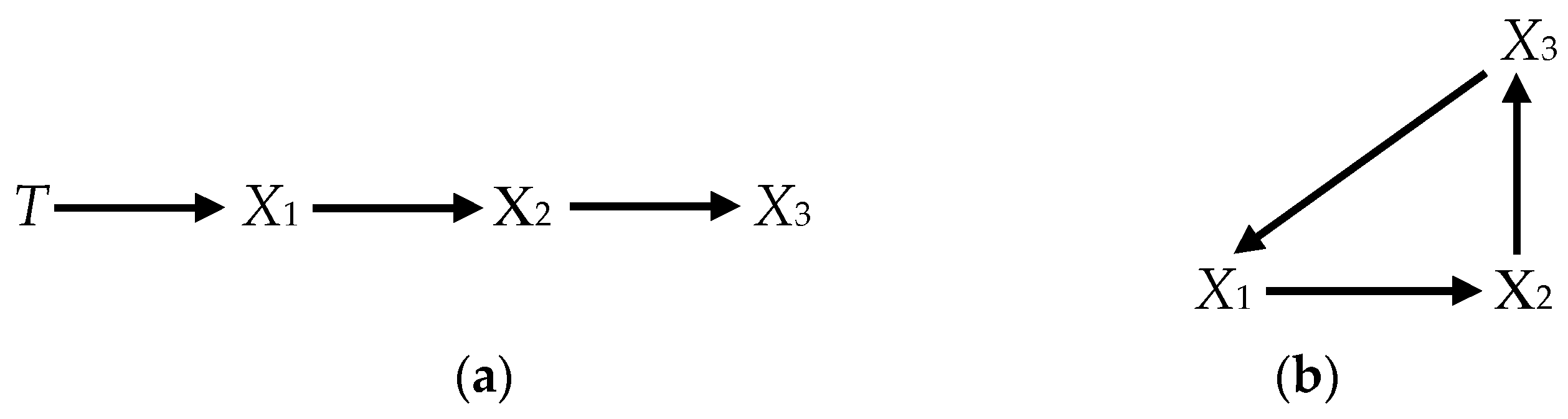
The nonstationarity of the variables in a system of equations such as Equation (1) may arise in two ways. Consider two distinct DGPs. Assume that there are two sets of variables, Xt and Tt. The first corresponds to the graph Figure 1a—a simple chain:
where the Ts are exogenous I(1) trends
and the ε’s and the η’s are identically, independently distributed (i.i.d.) random shocks. The connection of DGP 1 to the CVAR of Section 2 will become clear presently.
The second distinct DGP corresponds to the graph in Figure 1b:
where the ζs are i.i.d. random shocks.
DGP 1 shows the first of the two ways that variables may display stochastically trending behavior: T trends stochastically independently of the other variables in the system because of its fundamental random-walk structure and transmits that behavior to the Xs, i.e., if the trend (T) did not appear in Equation (2), which was otherwise unaltered (i.e., ΦXX remaining the same), the system would not contain an autoregressive root of unity and the X’s be stationary).
Now suppose that the trends are latent in DGP 1, so that we observe only the Xs. To see what is implied for the cointegration of the Xs, we can solve out T to get a reduced form. The resulting system will have reduced rank (=2) and the cointegration space is spanned by two vectors given by8
DGP 2 shows the second way that variables can stochastically trend: here, the X’s trend, not because of an exogenous cause, but because of the fine-tuning of their structural coefficients (cf. Davidson and Hall 1991, p. 239). In particular, the parameters have been chosen specifically to give DGP 2 the same cointegration properties as DGP 1.9 It is important to understand that DGP 2 is not a reduced form of DGP 1. It is a distinct structural system that happens to have coefficients that give it the same cointegration properties as DGP 1. The fact that its variables display I(1) trends, reflects a system property of the model that cannot be reduced to the effect of any variables that would trend without the presence of the others. In contrast, in DGP 1, the Xs trend and are cointegrated because they are driven by the same exogenous I(1) trend; and that would be true whether or not the driving trend (T) were observed or latent.
The I(1) behavior of the variables in DGP 2 depends on the exact values of the elements of Π. It is fragile in the sense that a small change in one of the structural coefficients that does not reflect any change in the causal graph (Figure 1b) can result in the loss of cointegration and of the trend behavior of the Xs. In contrast, DGP 1 is generic in the sense that it is robust to changes in the values of the structural coefficients (i.e., to changes that do not alter the causal graph (Figure 1a)).
To illustrate, suppose that the coefficients of DGP 2 are altered, such that the values of Π in Equation (4) are now
where the bold entries indicate where Π has been altered. Now the rank(Π) is three, there is no cointegration among the variables, and, indeed, the previously nonstationary Xt are now stationary.10
In contrast, consider making changes of the same magnitude in the analogous part of the causal structure of DGP 1 in (2), so that
where again the bold numerals indicate the alterations. Unlike the case of DGP 2, qualitatively, the cointegration properties remain unchanged—there is still only the one trend, T, in the system. Again, if we take the trend to be latent, then, while the precise values of the cointegrating relationships have changed, the cointegration rank (2) has not. The cointegrating vectors are now
Cointegration in DGP 2 is fragile in the sense that only specific choices of coefficients produce a trend and cointegration, and small deviations from those values can destroy those properties. Cointegration in DGP 1 is generic in the sense that small deviations in coefficients, while they alter precise values of cointegrating relations, nonetheless preserve the cointegration rank (i.e., the number of trends). The generic nature of the cointegration properties of systems like (2) is the result of the trend behavior of the X’s having an independent cause based in exogenous variables that are fundamentally I(1), while the fragility of cointegration in a DGP like (4) is the result of it arising only from the fine-tuning of the structural coefficients. Such fine-tuning could arise in specific cases for good economic reasons; however, in the spirit of Reichenbach’s Principle of the Common Cause, we should assume that it would not be the general case, unless we can point to an economic explanation of why the structural coefficients take those specific values in a particular case.11 It is unlikely that cointegration generally arises from a fortuitous combination of coefficients, which combined with the fact that we often find cointegration among the observable variables without any of them being weakly exogenous, suggests that the source of nonstationary behavior and cointegration among observable variables is more typically the result of latent I(1) trends.
In DGP 1, we can point to specific variables that are the source of the trends. In this case, we will say that the variables are driven by genuine (or real) fundamental trends, whether those trends are themselves observed or are latent. It is conventional in the CVAR literature to say that any system of I(1) variables with reduced-rank contains trends equal to the number of variables in the system less the number of cointegrating relations (the rank). These trends may generally be represented as the cumulation of the permanent shocks to the CVAR, which are backed out of the shocks to the Xs by imposing identifying assumptions (see Juselius 2006, chp. 15, especially Section 15). These representations are generally not uniquely identified, even when there are latent fundamental trends in the DGP and even when, as in DGP 2, there are no fundamental trends at all. In either case, we might call them “virtual trends,” since they do not correspond to a particular variable—observable or latent.
Our working hypothesis is that trending behavior originates economically in a relatively small number of variables whose own natures are such that they are nonstationary; we call these “fundamental trends.” The number of fundamental trends causally influencing a set of variables is equal to q (the number of variables (p) minus the rank of the Π matrix (r)). However, the fundamental trends themselves may or may not be among the observed variables. Other variables may be nonstationary, because these fundamental trends are among their direct or indirect causes; we call these “ordinary (nonstationary) variables”. In most cases, it would seem that we observe only ordinary variables, and the ultimate source of their trending behavior is to be found among their latent causes.
It might be argued that DGP 1 is also fragile because a change of parameters that rendered any of Ts stationary would upset the cointegration properties of that model in the same way that those of DGP 2 are upset by a small change in coefficients. However, that would miss the essential point. Of course, if the exogenous Ts were not I(1), then there would be no trends to transmit. The argument here, however, is that, in a structural model, it is far more likely that the source of a trend is a particular I(1) variable—either observed or latent—than that the source would be a group of distinct structural equations that just happen to have the right coefficients to generate what very often are multiple I(1) trends. This is ultimately not an econometric argument, but an economic one—we can more easily think of good economic reasons that a single economic variable might be a random walk (or a random walk with a drift or a random walk with a deterministic trend) than we can think of good reasons that that the parameters of several equations are appropriately tuned. For example, common sense and experience suggest that it is highly unlikely that a small change in the relative weights that a central bank places on inflation and unemployment in its reaction function would fundamentally change the cointegration properties of a system of structural macroeconomic equations. If we do not observe such instability of the cointegration properties and we most often do not find observed exogenous I(1) variables, then it suggests that typical estimated CVARs are reduced forms and that we will have to dig deeper to discover the structure that lies behind them. Ultimately, this is an empirical hypothesis about whether CVARs based on structures like DGP 1 prove to be more economically informative than those based on structures like DGP 2. Our goal is to explore some of the implications of this hypothesis about of the typical origin of I(1) trends for the long-run causal structure of the world and for the possibilities of uncovering that structure (or, as least, parts of it) empirically.12
4. Graphical Analysis of the CVAR
The DGP that adequately represents the long-run causal structure in the economy is not directly observable. But might it be inferred on the basis of data and not simply imposed as a priori restrictions on the CVAR? We begin by showing, first, how a DGP can be represented as a causal graph; and, second, how we can think of that graph as a map of the transmission of trends through the system of variables. We then want to investigate whether the facts of cointegration and weak exogeneity among subsets of observable variables might provide the necessary empirical data to allow us to recover reliable information about the underlying DGP, analogously to the way in which graphical causal search algorithms allow us to infer the causal structure of stationary data from empirical evidence about probabilistic dependence and independence among subsets of variables. The two critical tools are Davidson’s (1998) analysis of irreducibly cointegrating sets of variables and Johansen’s (2019) state-space analysis of the CVAR, which provides an instrument for analytically determining weak exogeneity among subsets of variables. These tools allow us to explore the logic of causal inference for nonstationary data. In Section 5, we demonstrate applications of that logic that suggest a possible basis for a causal search algorithm.
4.1. The Canonical CVAR of a Causally Sufficient, Acyclical Graph
Consider first the long-term structure of a causally sufficient CVAR with an acyclical causal structure in which the fundamental trends are represented explicitly. In the remainder of the paper, we consider only cases for a strong form acyclicality in which we do not permit any feedback from one variable to another, even with a time delay. Thus, we rule out cases such as Xt → Yt+1 → Xt+2.
The DGP is given as
where ; T is a q × 1 vector of fundamental trends; X is a p × 1 vector of ordinary variables, which may be trending (i.e., I(1)), but are not fundamental trends; is a (p+q) × 1 vector of shocks to ordinary variables (εit, t = 1, 2, …, p) and to fundamental trends (ηjt, j = 1, 2, …, q), each of the elements of which is an identically independently distributed random shock, and , where Ω is diagonal.
The system can be partitioned as
where the submatrix of parameters is full rank p × p, while is p × q, is q × p, and is q × q.
Because X is the vector of ordinary variables, is full rank and the eigenvalues of Ip + ΨXX must be less one in absolute value.13 If the variables in T are the actual I(1) fundamental trends, as opposed to ordinary variables that serve as the conduits of the fundamental trends into the observable system, they must be mutually causally independent, requiring ΨTT = 0qq, and strongly exogenous, requiring ΨTX = 0qp (Johansen 1995, p. 77; Juselius 2006, p. 263).
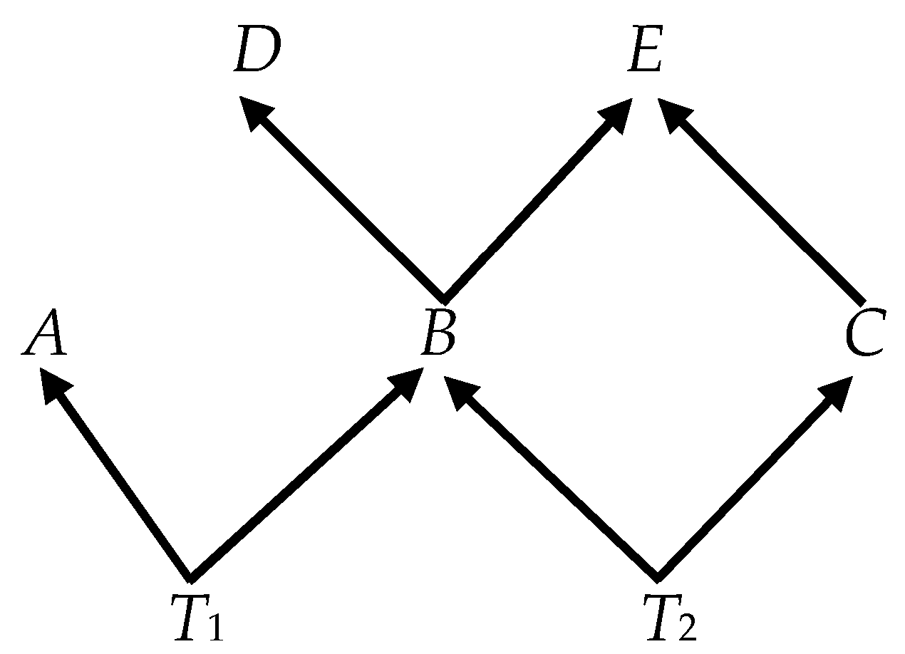
The Ψ matrix in (5) can be decomposed analogously to the Π matrix in (1) such that Ψ = αβ′, where α is (p + q) × r and β′ is r × (p + q). The transitional causal structure embedded in Ψ that governs the transmission of shocks and ultimately determines the long-run causal structure reflected in (25) can be represented in this αβ′-decomposition in the following canonical way—variables that are both cointegrated and directly causally connected are represented by the individual cointegrating relations expressed in β and the effects of causes are indicated by non-zero coefficients in α. To take a concrete example, consider a specific causal structure embedded in a DGP like (5) and represented graphically in Figure 2. (With causal time-series graphs, we suppose henceforth that the arrows correspond to a one-period lag between a direct cause and its effect.)
Thus, the causally canonical representation of Figure 2 would be given as
The rules governing the translation of the Figure 2 or any graph into the a DGP analogous to (7) are straightforward:
- Each single-variable direct causal pair or each collider is represented by a cointegrating relationship corresponding to a unique row of the β′ matrix where the value of the parameter for the effect is normalized to unity;
- There are as many adjustment parameters in α as there are rows in β′ (at most one per row) with the column of each non-zero parameter in α corresponding to the row of one of the effects (i.e., corresponding to the row in which that variable is normalized to unity) in β′;
- If any variable is a cause, but not an effect with respect to all the other variables, it corresponds to a zero row in α (and, thus, is weakly exogenous).
The β matrix thus tells us which variables are related causally and, therefore, connected by edges, and the α matrix (equivalently the normalization of β′) tells us which way the arrows point for those edges.
Except for trivial reorderings of the variables and rescalings, the DGP (7) uniquely represents the causal graph in Figure 2. Algebraically, however, the matrices α and β are not unique. They can be rotated to form other pairs (α* and β*) such that Ψ = α*β*′. The αβ′—representation and the α*β*′—representation yield the same value of the likelihood function. The problem of causal search is to find empirical information, other than the value of the likelihood function, that would allow us to select the canonical representation as in DGP (7) that corresponds to the graph of the data-generating process.
4.2. Formation and Sharing of Local Trends
We can think of the causal graph of a system of I(1) variables as representing the channels of transmission of these trends. Each collider corresponds to the creation of a local trend, and the causal variables involved in the collider are cointegrated with the effect variable. The transmission of a local trend from one variable to a single other variable also implies the cointegration of the cause and the effect.
Although causal connections produce cointegration, cointegration itself is not essentially a causal notion. Instead, cointegration results either (a) when a local trend is shared by two variables or (b) whenever the number of variables sharing the same fundamental trends, whether or not they share the same local trends (i.e., whether or not they share the fundamental trends in the same proportions), exceeds the number of fundamental trends. Thus, in case (b), if there is a set of variables each of which is driven by the same q fundamental trends, then any q + 1 of them will be cointegrated. A causal connection is, thus, sufficient for the cointegration of the complete set of causes with their effect, but it is not necessary.
Proposition 1.
Causal Cointegration: If each member of the set of parents of a variable C in a causal graph is I(1), then the set of variables consisting of C and its parents, is cointegrated.
It is convenient to write the fact that a set of variables is cointegrated as CI(Z), where Z is a set of variables with two or more members. Thus, if the variables A and B are cointegrated, we can write this as CI({A, B}). Two terms will prove useful:
Definition 2.
A cointegrating group is a set of variables in which every pair of variables shares the same common local trend—i.e., every pair is cointegrated.
Definition 3.
A collider group is a set of variables consisting of a variable C and the complete set of its parents.
The variables in a cointegration group share a single common local trend; while the variables in a collider group generate a new local trend at C. The same variable may be part of both a cointegration group and a collider group. Other sets of cointegrating variables may be in neither type of group. Davidson (1998, p. 91) introduces a useful concept, which we define here slightly differently that he does.
Definition 4.
A set of variables is irreducibly cointegrating (notated IC(.)) if, and only if, it does not contain a subset that is itself cointegrated.
4.3. A State-Space Analysis of the CVAR
It will prove useful to examine the relationship between weak exogeneity and the causal graph. Weak exogeneity is not in itself a causal property; rather, it is a property related to the manner in which a likelihood function can be decomposed into a conditional and marginal probability distribution under a given parameterization (Engle et al. 1983). Although weak exogeneity is important because it is turns out to be the condition that guarantees that the parameters of interest can be efficiently estimated, we are not interested in the current paper in efficient estimation. Rather we want to show how zero rows in α in the CVAR for subsets of variables, known as “weak exogeneity” conditions, can reveal information about the causal structure of the DGP.
Given a DGP, the weak exogeneity status of its variables will depend on the model we estimate. So, for example, if (7) were the DGP with ψij ≠ 0 and we estimated a CVAR with precisely the form of the DGP with ψij unrestricted, then the variables T1 and T2 would be weakly exogenous in the model for {A, B, C, D, E, T1, T2}t+1 given {A, B, C, D, E, T1, T2}t for the coefficients ψij or (αji, βij), i = 1, 2, …, 5, j = 1, 2, …, 7. Our main interest, however, will be in the case in which only a subset of the variables is observed—leaving other variables in the DGP latent. So, for example, we might consider data generated by (7) but observe only B, C, and E. These variables can be modeled in a CVAR form, but the coefficients of the model will not in general be the same as those of (7), though we could compute them if we knew the DGP. Still, we can ask the question whether we can decompose the likelihood function of this model, with some unobserved variables, in a manner that renders some of the observed variables weakly exogenous with respect to the coefficients of a conditional model for the remaining observable variables.
We can notate this weak exogeneity using a new symbol “↦”, which means “is weakly exogenous for” and is to be distinguished from “→,” which means “directly causes.” Thus, X ↦ Y can be read as “the variables in the set X are weakly exogenous for the coefficients of a CVAR model of Y conditional on X” or, leaving the relativity to a particular set of parameters implicit, “X is weakly exogenous for Y.” If we know the causal graph of the DGP, then we can read the various weak exogeneity relationships for models of different subsets of variables from information in the causal graph. As a result, if we can identify weak exogeneity relationships for different subsets, we may be able to work backwards to determine which causal graphs could have generated them.14
The object of the analysis is to use tests of long-run weak exogeneity in CVARs of the form of Equation (1) applied to only the observable variables to discover restrictions on allowable causal ordering of the underlying DGP (6). Long-run weak exogeneity corresponds to a zero row in the α matrix of the CVAR, so a critical goal is, given a particular DGP, to determine what it implies for the α matrix of a CVAR of the subset of observable variables (Johansen 1995, Section 8.2.1; and Juselius 2006, Section 11.1).
Johansen (2019) provides a state-space analysis of the DGP of a CVAR that allows us to determine analytically what statistical tests of weak exogeneity should find (given sufficient data and so forth) for different subsets of observable variables. Fundamental trends are assumed to be latent. In order to analyze weak exogeneity among subsets of variables, Johansen partitions the ordinary variables Xt = [X1t, X2t] into those that are in the subset of interest X1t (referred to as observed) and those outside the subset X2t (referred to as the unobserved). Then, rather than partitioning Ψ as in (6), partition it as , where the submatrices of parameters may or may not coincide with the Ψij, depending on whether any ordinary variables are unobserved. The m × p null element in the lower left-hand corner of the Ψ matrix corresponds to the assumption that the fundamental trends are strongly exogenous, and the m × m null element in the lower right-hand corner indicate that fundamental trends do not cause one another.
The submatrix contains the parameters of the ordinary variables. Only the parameters in M11 relate exclusively to the p1 observed ordinary variables, while the other Mij contain parameters that relate partly or exclusively to the p2 latent ordinary variables. The submatrix contains the coefficients in that relate to the effects of the latent fundamental trends on the observed ordinary variables and those in that relate to the their effects on the unobserved ordinary variables.
A state-space representation of DGP (6) can then be given.
where t = 0, 1, .…, n − 1, and T0 = 0 and X0 = 0. The shocks are partitioned into those affecting ordinary variables (ε) and those affecting the latent variables (η), with (εt, ηt) ~ i.i.d. Np+m(0, Ω), , where Ω is diagonal. In keeping with the distinction between ordinary variables and fundamental trends, we assume that the eigenvalues of Ip + M, Ip1 + M11, and Ip1 + M22 are less than one in absolute value, so that the source of the nonstationarity of Xt is the fundamental trends rather than its own dynamics.
The matrix C represents the proportions of fundamental trends present in observable variables but transmitted to them through latent causal connections and not via causal relationships among the observable variables. Thus, while the non-zero entries of M correspond to the edges in a causal graph, C is not given a direct graphical interpretation. The fundamental trends are embedded in T, but the variables included in T should be regarded as local trends, which may either be latent fundamental trends directly causing the observed variables or latent ordinary variables that carry some linear combination of fundamental trends and cause the observable variables. Therefore, while we have assumed that Ωη is diagonal, it need not be (and the conclusions about weak exogeneity in the next subsection would be unaffected).
Suppose that the DGP is described as in systems (8)–(10), and we wish to know whether any of the observed variables (X1t) are weakly exogenous in a CVAR of the observed variables only. This comes down to the question of whether α in that CVAR has any zero rows. Johansen proves that the α of such a CVAR can be written as
where the conditional variances are
and the long-run variances are
see (Johansen 2019, Sections 2 and 3, especially Equations (12) and (13), Theorem 3, and Equation (18)).
In the simpler case, in which all variables are observed (i.e., there are no X2’s), Johansen (2019, Section 3, Case 1) shows the formula in Equation (11) can be made even simpler:
4.4. Weak Exogeneity and Causal Order
Johansen’s (2019) state-space representation and his Theorem 2 offer a tool for analyzing weak exogeneity for subsets of variables in the DGP. These, in turn, correspond in systematic ways to facts about the causal structure of the DGP itself. Consider some illustrative cases:
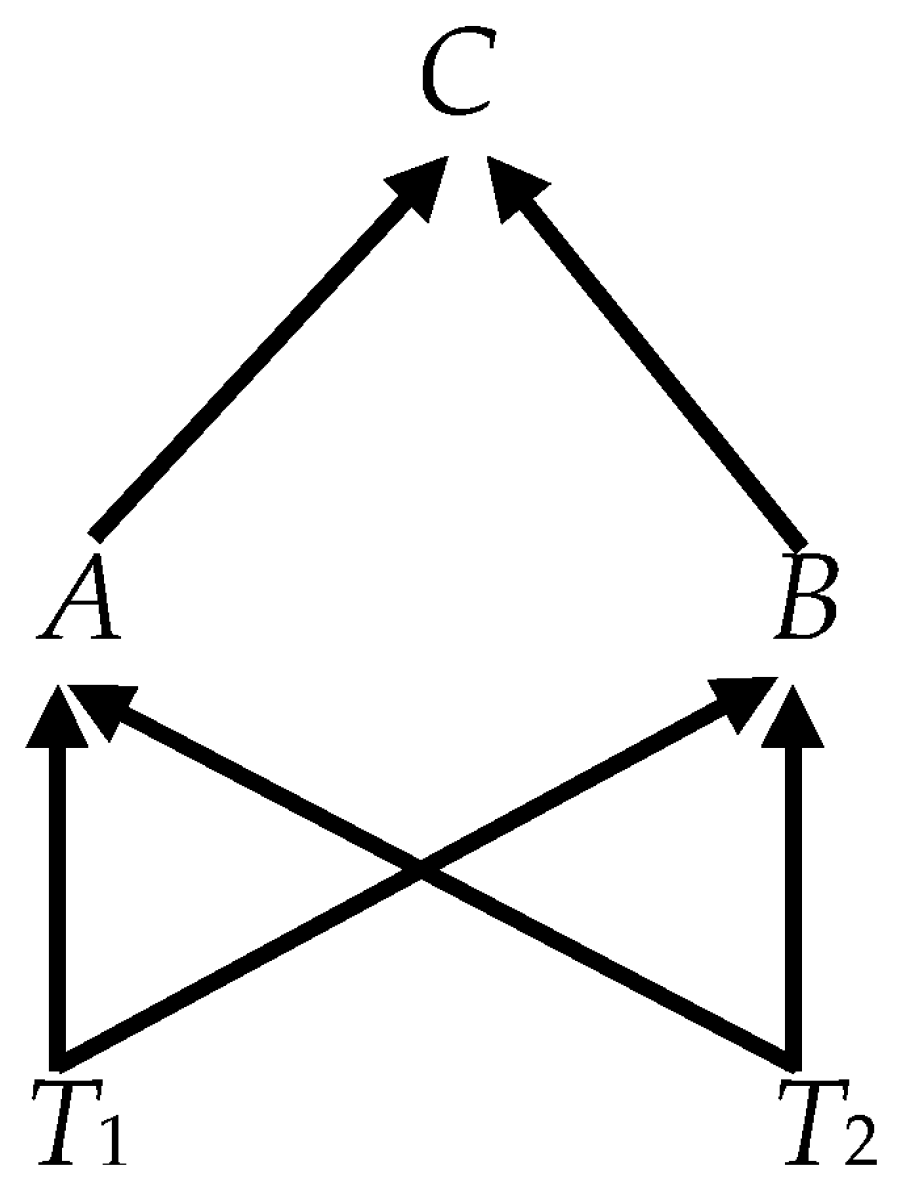
- Case 1.
- Consider the causal graph in Figure 3, in which all ordinary variables are observed and only the fundamental trends are unobserved, so that (12), the simpler formula for α, applies. The DGP in Equations (8)–(10) specializes towherewhere ωii = var(εit), i = A, B, C;Thus,where the asterisk (*) indicates a non-zero value.15 The first two rows of α are zero and, therefore, A and B are weakly exogenous for C (i.e., {A, B} ↦ C). Notice that it does not matter, what the causal relations are among the observables, since they are encoded in the M11 matrix, which plays no part in the determination of α in Equation (11). What matters is which variables convey the fundamental trends to the observables.
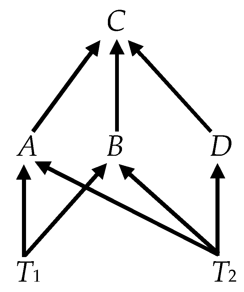
- Case 2.
- Unfortunately, the simple mapping between weak exogeneity and causal connection suggested by Case 1 does not hold up. Consider Figure 4, which adds the variable D and edges connecting it to other variables in Figure 3. The analysis proceeds just as in Case 1. Again, since all variables are observable, the simpler formula (12) applies. The other relevant matrices of the state-space formulation are given byThese imply thatwhich has no zero rows; which, in turn, implies that none of the variables is weakly exogenous.16 The variables A, B, C, D are cointegrated (CI({A, B, C, D})); but with two fundamental trends and four variables, every three-member subset of the ordinary variables is also cointegrated, implying not IC({A, B, C, D}). This appears to be a robust finding—the parents in a collider are weakly exogenous only when the colliding set is irreducibly cointegrated.
- Case 3.
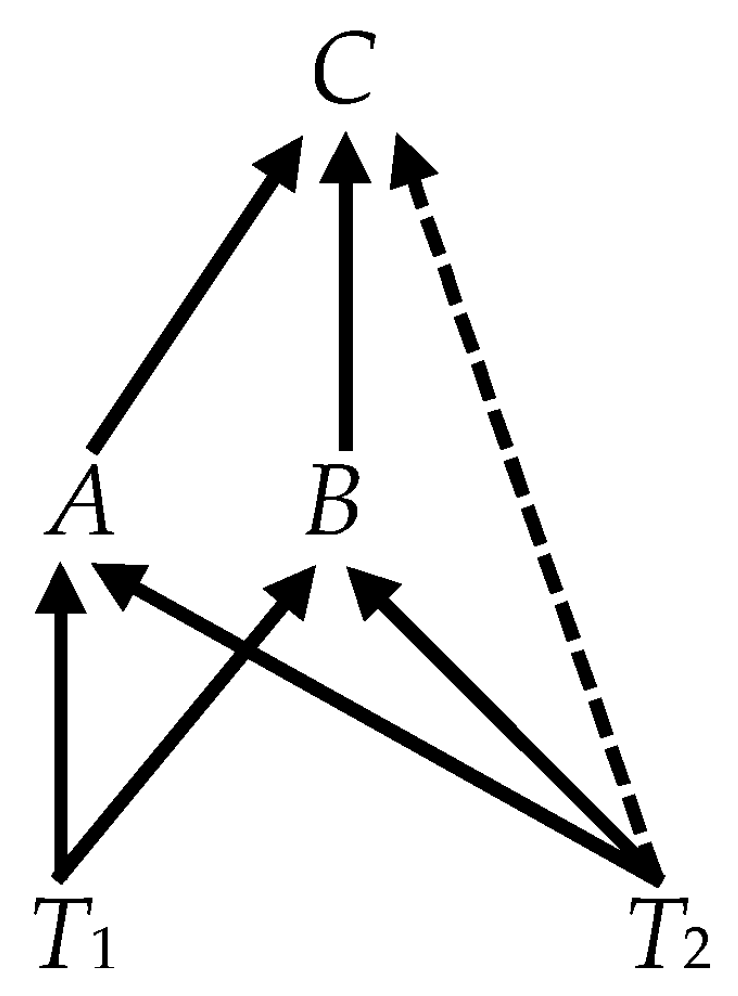
- It is tempting to think that we might consider an irreducible subset of the variables in Figure 4, such as {A, B, C} and find the same weak exogeneity relations as we did in Figure 3. That, however, does not work. In analyzing the subset, we are effectively treating D as an unobserved variable; and we must, therefore, apply the more general formula (11), which requires additional information. The critical elements of the state-space representation of this reduced system areand(Note that, although is diagonal by assumption, the off-diagonal elements of VTT here are nonzero. This is the result of D, transmitting T2 to the collider at C. The calculation of V (see Equation (11)) conditions {D, T1, T2} on {A, B, C} and, in effect, conditions the independent (distal) causes T1 and T2 on their common (indirect) effect, which induces probabilistic dependence between them.) The variance of the isandWith no zero rows in α, none of the variables is weakly exogenous. Although D is unobservable in the DGP that actually determines the value of the observable variables, it provides a conduit from the fundamental trends to C that is distinct from the observable conduits, A and B. It is as if the graph of Figure 4 has been transformed into Figure 5, where the dashed arrow indicates a causal connection between T2 and C, mediated by D in the DGP but not observable in the CVAR of the subset {A, B, C}. Unobserved mediating causes, like D, can make an indirect causal connection appear to be direct.
- Case 4.
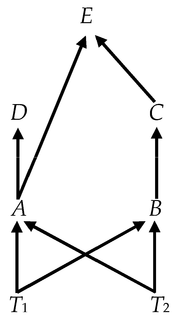
- In Case 3, weak exogeneity failed to obtain, even though the causal connections were genuine. It can also happen that weak exogeneity does obtain, even when causal connections are missing. Consider Figure 6. The graph shows not (A → C) and not (B → D) and not (B → E), although B does indirectly cause E. Using the same state-space methods, but omitting the details here, we can show that {A, B} ↦ {C, D, E}. And, looking at subsets of variables {A, B} ↦ D. Thus, {A, B, D} have the same apparent pattern of weak exogeneity as found for {A, B, C} in Case 1 (Figure 3); yet these variables do not form a collider group in Figure 6. But notice CI({A, B, D}), but also CI({A, D}). The set {A, B, D}, therefore, is not irreducibly cointegrated. It appears that a mapping between weak exogeneity and causal connections can be established only in irreducibly cointegrated sets.
- Case 5.
- Weak exogeneity may fail to track direct cause. Consider a causal chain:All four observable variables form a single cointegration group, sharing the single fundamental trend. Note that B ↦ C and that {B, C} form a cointegration group. We might be tempted to conclude that these facts would warrant inferring what is, in fact, true that B → C. A similar case shows the problem: A ↦ C and CI({A, C}); but, in fact, it is not true that A → C (A is an indirect, but not a direct, cause of C). It is worth showing why it is the case that A ↦ C, as it highlights a subtle issue. We take {A, C} to be observed and {B, D} to be unobserved. Then the relevant matrices areT → A → B → C → D
The variance of the is
and
The zero row in α implies that A ↦ C. The result hinges crucially on V2T being a zero matrix. This is, in turn, implied by the fact that A screens off B and D from T in the graph. Conditioning on the screening variable A as is done in the calculation of V2T renders both B and D probabilistically independent of T.
Using a similar analysis, it is also easy to show that the subset {B, D} displays the same pattern as {A, C}: B ↦ D and CI({B, D}), yet it is not true that B → D. The example shows that we have to be careful in making such inferences, but not that they are hopeless. Note that we can show that A ↦ {B, C, D}; B ↦ {C, D}; and C ↦ D; so that the variables form a nested hierarchy with A at the top. This hierarchy can be reinterpreted as a chain: A ↦ B and all variables lower in the hierarchy; B ↦ C and all variables lower in hierarchy; C ↦ D; and D is not weakly exogenous for any variable. Such as chain recapitulates the causal graph. The lesson is that a when a variable is weakly exogenous for another variable in a cointegration group, it is a direct cause only if it is adjacent in the sense of sitting at the immediately higher step of the hierarchy.
Although we have not provided a proof, these cases suggest how to read weak exogeneity off a causal graph. There are four conjectured criteria:
- Within a set of variables that form a cointegration group, a particular variable is weakly exogenous for the group if, and only if, it is the sole source of the local trend that cointegrates the group;
- The parents in any set of variables that form a collider group in which two or more local trends are combined are weakly exogenous for the child in the collider group, provided that the number of variables in the group is fewer than one plus the number of fundamental trends carried by those variables;
- If a collider fulfills criterion B, then in any set that replaces one or more weakly exogenous parents with a variable in the same cointegration group as that parent, provided the variable is itself weakly exogenous for the parent, will also be weakly exogenous for the child. (Thus, in Figure 6, in the collider {A, C, E}, {A, C} ↦ E; but in the set in which B replaces C (both in the same collider group), {A, B} ↦ E));
- If a collider fulfills criterion B, then any variable that is weakly exogenous for the child, either as a parent or as a member of the same cointegration group that replaces the parent, will be weakly exogenous for a variable that replaces the child from a cointegration group that includes the child and for which it is weakly exogenous. (Thus, in Figure 2, {T1, T2} ↦ B, but in the set that replaces B with D, which are both in the same cointegration group, {T1, T2} ↦ D.)
The inferential lessons of Cases 1–5 can be summarized in three conjectured rules, consistent with visual reading of the graph:
Rule 1.
If A ↦ B, then not B → A.
Rule 1 simply says that causation cannot run against the direction of weak exogeneity.
Rule 2.
In a cointegration group, if A ↦ B and there is no C such that A ↦ C and C ↦ B, then A → B.
Rule 2 says that bivariate weak exogeneity coincides with direct causation, provided that the variables are adjacent.17
Rule 3.
A set of variables W with k ≤ q members forms a collider at one of its members (call it variable C), if (i) IC(W); (ii) W-C ↦ C, where W-C is the set W omitting C; (iii) it is not the case that any member B ∈ W-C is a member of a cointegration group Z such that, for any member D ∈ Z (excluding B), B ↦ D and W-B+D ↦ C, where W-B+D is W with D taking the place of B; and iv) it is not the case that C is a member of a cointegration group Z such that for any member E ∈ Z (excluding C) that E ↦ C.
Rules 3 says that if a set of k + 1 variables is irreducibly cointegrated and k variables are jointly weakly exogenous for the k + 1th variable, then they form a collider, provided that each of the weakly exogenous variables is adjacent to the third variable (established by conditions (iii) and (iv)).
5. The Basis for a Long-Run Causal Search Algorithm?
The DGP that adequately represents the causal structure in the economy is not directly observable. Might it be inferred on the basis of data and not simply imposed as a priori restrictions on the CVAR? Based on our analysis of long-run causal structure, can we recover reliable information about the underlying DGP from the facts of cointegration and weak exogeneity analogously to the way in which graphical causal search algorithms infer causal structure for stationary data from empirical evidence about probabilistic dependence and independence among subsets of variables?
Davidson (1998, Section 3) proposes a search algorithm that identifies every irreducible cointegrating set of variables within a CVAR. He then uses that information where possible to identify the cointegrating relations in the β′ matrix. This strategy is successful in some cases and not others. There is an analogy with causal search for stationary variables. Despite the slogan, “correlation is not causation,” it is sometimes possible to infer causal direction from tests of unconditional dependence. For example, for a causally sufficient set of three stationary variables with an acyclical data-generating process, if A and C are not correlated, but A and B and B and C are correlated, then A → B ← C is the only consistent causal graph. In most cases, however, unconditional independence is not enough. Relations of conditional dependence and independence provides a richer source of information for inferring the direction, as well as the existence of causal edges (see Section 2.2 above).
Davidson’s schema places cointegration in something like the logical role of unconditional independence (or correlation) in the stationary case. The analysis of Section 4 suggests that Davidson’s inferential scheme can be further developed by explicitly recognizing, first, that the ultimate source of nonstationarity in any set of variables is often found in latent trends and, second, that assessment of weak exogeneity may provide evidence of causal asymmetry. Within irreducibly cointegrated subsets of the variables, weak exogeneity can function in something like the logical role of conditional independence, when processed according to the three rules of Section 4.4, and may provide richer, empirically grounded information about the identification of the CVAR. As with causal search in the stationary case, the application of these rules is unlikely to identify every possible causal graph but may sometimes be able to partially or completely uncover the underlying causal structure.
To illustrate, we analyze two cases—one with and one without causal sufficiency.
5.1. Long-Run Causal Search in a Causally Sufficient Graph
Consider the DGP in Figure 2 and assume that its variables are causally sufficient and all (including the fundamental trends) are observed. We are interested in the logic of causal inference rather than the statistical problem of inference, so we also assume that prior statistical testing has successfully identified the facts with respect to the cointegration rank of the system and cointegration and weak exogeneity among any subset of variables. (In the language of the causal search literature, we assume that we have an oracle.) Naturally, in practice our inference cannot be more certain than the statistical inferences that provide our assumed facts. Can we use this information to recover the graph of the DGP?
The inference problem can be viewed as how to place the zero and non-zero coefficients in the α and β′ matrices in Equation (7).
Given that we know that the cointegration rank is 5, we know that there are two fundamental trends. This implies that α is 7 × 5 and β′ 5 × 7. Since T1 and T2 are weakly exogenous with respect to all other variables in the system, we may conclude that, even if they are not identical with the fundamental trends (which in this case, of course, they are), they are at least the unique sources introducing those trends into the system. And we are entitled to enter zeroes in the entire rows of α corresponding to T1 and T2. Without loss of generality, we may enter non-zero αijs along the main diagonal of the submatrix of α, excluding the T1- and T2-rows, and zeroes everywhere else. Similarly, we may enter ones on the main diagonal of the submatrix of β′ that excludes the last two columns.
With two fundamental trends, no irreducible cointegrating relation can involve more than three variables. Exhaustive consideration along Davidson’s lines would produce 21 possible cointegrating pairs and 35 possible cointegrating triples. Similarly, we need to consider possible weak exogeneity of variables within each irreducibly cointegrating subset. Most of subsets are not irreducibly cointegrating or do not contain weakly exogenous variables, so rather than tediously listing the weak-exogeneity status of all 56 subsets systematically, we just note the salient ones.
From the facts that CI({A, T1}) and that there are no other variables in this cointegration group and that T1 ↦ A, Rule 2 implies T1 → A, which justifies the placement of in row 1 of β′ and zeroes in the remaining unassigned places in that row. Analogous reasoning with respect to {C, T2} implies T2 → C and justifies the placement of and the zeroes in row 3. Again, with respect to {B, D}, analogous reasoning justifies the placement of and the zeroes in row 4. In addition, in this case, Rule 1 and the fact that B ↦ D imply that not (D → B) and justify the zero in row 2, column 4.
Rule 3 and the facts that IC({T1, T2, B}), that B is not part of a cointegration group with either T1 or T2, and that {T1, T2} ↦ B allows us to identify the collider T1 → B ← T2 and justifies the placement of and and the remaining zeroes in row 2 of β′.
Rules 3 and the facts that IC({B, C, E}), ({B, C} ↦ E, and not (C ↦ T2), with which it forms a cointegration group, allows us to identify the collider B → E ← C and justifies the placement of and and the zeroes in row 5 of β′. With that, we were able to recover the entire DGP graph using only the facts of cointegration and weak exogeneity.
5.2. Long-Run Causal Search in the Presence of Latent Trends
The CVARs typically estimated in practice most often do not contain variables that are weakly exogenous for the whole system, which could, therefore, be identified as the conduit of the fundamental trends to the other variables in the system. It is, therefore, worth considering how the principles of search might operate when fundamental trends are latent variables. It is possible to apply the rules of Section 4.2 to the variables generated according to Equation (7) when only the ordinary variables (A, B, C, D, E), but not the fundamental trends (T1 and T2), are observed.
For some of the causal edges, the reasoning of Section 4.3 is still applicable, and we would be able to infer the edges shown in Figure 7: B → D and B → E ←C. The remainder of Figure 7 requires further comment.
We are unable to infer the edges between T1, T2 and A, B, and C for the simple reason that the two fundamental trends are not observed and the inference of the edges in which they are involved requires their observability. However, we do know from the fact that the cointegration rank is 3 that there are two fundamental trends. What we cannot say, however, is precisely how those two trends enter directly into the observable system. They may, in fact, be transmitted through ordinary variables that are also latent. We do know that they must enter through A, B, or C. If that were not the case and a fundamental trend entered through D or E, we would not have found that CI({B, D}) or {B, C} ↦ E. This is indicated in Figure 7 by the oval enclosing the ordinary variables and the circles (indicating their latency) around the fundamental trends. The arrows running from the latent fundamental trends to the oval, stopping short of the particular variables indicates that we know that these variables are caused by these trends, albeit we do not know exactly what the connections are. Thus, instead of (7), we can fill in the causally ordered CVAR Equation (15) with the ambiguous information depicted in Figure 7, where the question marks indicate parameters that correspond to possible, but yet-to-be-determined causal edges.
Equation (15) depicts what observables imply about the DGP and not just facts about the observables themselves. Here the two trends are not observable, but we know that there are two latent trends because none of the observable variables is weakly exogenous when one considers the whole set of observable variables, which again justifies the placement of the two zero rows in α.
Neither the graph nor (15) conveys all the information that we have. We know, for instance, that there are two fundamental trends and that at least one of the fundamental trends must causally influence each of A, B, and C. If that were not so, then the only way that all three variables could carry the trends and be irreducibly cointegrated would be for them to form a collider group in which one pair is weakly exogenous for the remaining variable. Given the DGP, we know that the weak exogeneity search should not find such a pattern. Furthermore, we know that no two of A, B, and C could have a common latent cause. If that were not true, that pair would form a cointegration group, which, given the DGP, the search for cointegrating pairs should not find such a cointegration group. These two conclusions imply that each of the three observed variables carries the fundamental trends in distinct proportions. These facts place restrictions on how the last two columns of the β′ in (15) can be filled in to be consistent with the DGP. In particular, in 3 × 2 submatrix in the upper right-hand corner of β′, at least one row must contain two nonzero entries and the remaining two rows cannot have zeroes in the same column. This guarantees that the variables A, B, C form a cointegration group without also forming a collider group with weakly exogenous parents.
6. Conclusions
In the history of econometrics, the problem of identification and the notion of causal order have long been connected—both in the work of Simon and the early Cowles Commission program and in the literature on SVARs. Typically, economists have relied heavily on the idea that a priori restrictions derived somehow from economic theory would provide the needed identification. Recent work on graphical causal modeling, however, has shown that there is often unexploited information that could provide a firmer, empirical basis for identification. In the case of cross-sectional data or the contemporaneous causal orderings of SVARs, the graphical causal modelers have stressed the information contained in conditional independence relationship encoded in the probability distribution of the data. Conditional independence may also be a resource in the case of the long-run dynamics of the CVAR, although the fact that nonstationary data involves non-standard distributions poses some challenges. We have suggested here that nonstationary data also present the opportunity to take a different approach.
Where do the trends we observe among macroeconomic variables come from? We showed that it is possible for the structure of the DGP to be such that a set of observable variables trends without any fundamental trends acting as drivers. Yet, we have argued that these cases rely on particular configurations of coefficients that are likely not to be robust to small changes in coefficients and that call out for an economic explanation of why they arise at all. Once a distinction is drawn between fundamental trends and ordinary variables, it is clear that a more robust account for nonstationary behavior is that it is transmitted from its fundamental sources to variables that without these fundamental trends as direct or indirect causes would not naturally be nonstationary. In typical CVAR analysis, econometricians mostly do not find variables that themselves can be identified as the source of fundamental trends. This suggests that, in most cases, fundamental trends are latent variables, and any sort of structural or causal analysis of CVARs must account for their latency.
We suggested—somewhat informally—that combining Davidson’s suggestion of a comprehensive search for sets of irreducible cointegrating relations with a similar comprehensive search of weak exogeneity among those sets could provide a non–a priori empirical basis for discovering identifying restrictions on cointegrating relations, as well as information on causal direction. We showed that in a simple example, the complete causal graph of the CVAR could be recovered. But, in most cases in the face of latent variables, these restrictions are unlikely to provide complete identification. Nevertheless, as in our illustration, some of the cointegrating relations may be identified, even when there are latent trends. It is also possible that, in some cases, it would be possible to recover estimates of the trends using state-space methods (see, e.g., Johansen and Tabor 2017). Finally, viewing the CVAR through the lens of latent fundamental trends reinforces Juselius’s advocacy of simple-to-general modeling in the CVAR context (Juselius 2006, Chapter 22, especially. Sections 22.2.3 and 22.3). Cointegrating relations are robust to widening the data set to include more variables. The aim of such widening can be seen as an effort to discover the observable variables that are the counterpart of the latent trends in narrower data sets.
Funding
This research received no external funding.
Conflicts of Interest
The author declares no conflict of interest.
References
- Cooley, Thomas F., and Stephen F. LeRoy. 1985. Atheoretical Macroeconomics: A Critique. Journal of Monetary Economics 16: 283–308. [Google Scholar] [CrossRef]
- Cooper, Gregory F. 1999. An Overview of the Representation and Discovery of Causal Relationships using Bayesian Networks. In Computation, Causation, and Discovery. Edited by Clark Glymour and Gregory F. Cooper. Menlo Park: American Association for Artificial Intelligence, Cambridge: MIT Press, pp. 3–64. [Google Scholar]
- Davidson, James, and Stephen Hall. l991. Cointegration in Recursive Systems. Economic Journal 101: 109–251. [Google Scholar] [CrossRef]
- Davidson, James. 1998. Structural Relations, Cointegration and Identification: Som Simple Results and Their Application. Journal of Econometrics 87: 87–113. [Google Scholar] [CrossRef]
- Demiralp, Selva, and Kevin D. Hoover. 2003. Searching for the Causal Structure of a Vector Autoregression. Oxford Bulletin of Economics and Statistics 65: 745–67. [Google Scholar] [CrossRef]
- Demiralp, Selva, Kevin D. Hoover, and Stephen J. Perez. 2008. A Bootstrap Method for Identifying and Evaluating a Structural Vector Autoregression. Oxford Bulletin of Economics and Statistics 70: 509–33. [Google Scholar] [CrossRef] [Green Version]
- Duarte, Pedro Garcia, and Kevin D. Hoover. 2012. Observing Shocks. In Histories of Observation in Economics. (Supplement to History of Political Economy 44). Edited by Harro Maas and Mary Morgan. Durham: Duke University Press, pp. 226–49. [Google Scholar]
- Engle, Robert F., and Clive W. J. Granger. 1987. Cointegration and Error Correction Representation: Estimation and Testing. Econometrica 55: 251–76. [Google Scholar] [CrossRef]
- Engle, Robert F., David F. Hendry, and Jean-François Richard. 1983. Exogeneity. Econometrica 51: 277–304. [Google Scholar] [CrossRef]
- Granger, Clive W. J. 1969. Investigating Causal Relations by Econometric Models and Cross-spectral Methods. Econometrica 37: 424–38. [Google Scholar] [CrossRef]
- Granger, Clive W. J. 1995. Commentary [on Stephen F. LeRoy, Causal Orderings]. In Macroeconometrics: Developments, Tensions, and Prospects. Edited by Kevin D. Hoover. Boston: Kluwer, pp. 229–352. [Google Scholar]
- Haavelmo, Trygve. 1944. The Probability Approach in Econometrics. Econometrica 12: iii–115. [Google Scholar] [CrossRef]
- Hood, William C., and Tjalling Koopmans, eds. 1953. Studies in Econometric Method. (Cowles Commission Monograph vol. 14). New York: Wiley. [Google Scholar]
- Hoover, Kevin D. 1990. The Logic of Causal Inference: Econometrics and the Conditional Analysis of Causation. Economics and Philosophy 6: 207–34. [Google Scholar] [CrossRef] [Green Version]
- Hoover, Kevin D. 2001. Causality in Macroeconomics. Cambridge: Cambridge University Press. [Google Scholar]
- Hoover, Kevin D. 2004. Lost Causes. Journal of the History of Economic Thought 26: 149–64. [Google Scholar] [CrossRef]
- Hoover, Kevin D. 2008. Causality in Economics and Econometrics. In The New Palgrave Dictionary of Economics, 2nd ed. Edited by Steven N. Durlauf and Lawrence E. Blume. London: Palgrave Macmillan. [Google Scholar] [CrossRef] [Green Version]
- Hoover, Kevin D. 2012. Economic Theory and Causal Inference. In Handbook of the Philosophy of Economics. volume 13 of Dov Gabbay, Paul Thagard, and John Woods, general editors. Edited by Uskali Mäki. Amsterdam: Elsevier/North-Holland, pp. 89–113. [Google Scholar]
- Hoover, Kevin D. 2014. On the Reception of Haavelmo’s Econometric Thought. Journal of the History of Economic Thought 36: 45–65. [Google Scholar] [CrossRef] [Green Version]
- Hoover, Kevin D. 2015. The Ontological Status of Shocks and Trends in Macroeconomics. Synthese, 3509–32. [Google Scholar] [CrossRef] [Green Version]
- Hoover, Kevin D., and Katarina Juselius. 2015. Trygve Haavelmo’s Experimental Methodology and Scenario Analysis in a Cointegrated Vector Autoregression. Econometric Theory 31: 249–74. [Google Scholar] [CrossRef] [Green Version]
- Hoover, Kevin D., and Òscar Jordá. 2001. Measuring Systematic Monetary Policy. Federal Reserve Bank of St. Louis Review 83: 113–37. [Google Scholar] [CrossRef] [Green Version]
- Hoover, Kevin D., Søren Johansen, and Katarina Juselius. 2008. Allowing the Data to Speak Freely: The Macroeconometrics of the Cointegrated Vector Autoregression. American Economic Review: Papers and Proceedings 98: 251–55. [Google Scholar] [CrossRef] [Green Version]
- Johansen, Søren, and Katarina Juselius. 2014. An Asymptotic Invariance Property of the Common Trends Under Linear Transformation of the Data. Journal of Econometrics 178: 310–15. [Google Scholar] [CrossRef]
- Johansen, Søren, and Morten Nyboe Tabor. 2017. Cointegration between Trends and Their Estimators in State Space Models and Cointegrated Vector Autoregressive Models. Econometrics 5: 36. [Google Scholar] [CrossRef] [Green Version]
- Johansen, Søren. 1995. Likelihood-based Inference in Cointegrated Vector Autoregressive Models. Oxford: Oxford University Press. [Google Scholar]
- Johansen, Søren. 2019. Cointegration and Adjustment in the CVAR(∞) Representation of Some Partially Observed CVAR(1) Models. Econometrics 7: 2. [Google Scholar] [CrossRef] [Green Version]
- Juselius, Katarina. 2006. The Cointegrated VAR Model. Oxford: Oxford University Press. [Google Scholar]
- Koopmans, Tjalling C., ed. 1950. Statistical Inference in Dynamic Economic Models. (Cowles Commission Monograph 10). New York: Wiley. [Google Scholar]
- LeRoy, Stephen F. 1995. Causal Orderings. In Macroeconometrics: Developments, Tensions, and Prospects. Edited by Kevin D. Hoover. Boston: Kluwer, pp. 235–52. [Google Scholar]
- Liu, Ta-Chung. 1960. Underidentification, Structural Estimation, and Forecasting. Econometrica 28: 855–65. [Google Scholar] [CrossRef]
- Morgan, Mary S. 1990. The History of Econometric Ideas. Cambridge: Cambridge University Press. [Google Scholar]
- Pagan, A. R., and M. Hashem Pesaran. 2008. Econometric analysis of structural systems with permanent and transitory shocks. Journal of Economic Dynamics and Control 32: 3376–95. [Google Scholar] [CrossRef] [Green Version]
- Pearl, Judea. 2009. Causality: Models, Reasoning, and Inference, 2nd ed. Cambridge: Cambridge University Press. [Google Scholar]
- Pesaran, M. Hashem, and Ron P. Smith. 1998. Structural Analysis of Cointegrating VARs. Journal of Economic Surveys 12: 471–506. [Google Scholar] [CrossRef]
- Pesaran, M. Hashem, and Yougcheoi Shin. 2002. Long-run Structural Modelling. Econometric Reviews 21: 49–87. [Google Scholar] [CrossRef]
- Phiromswad, Piyachart, and Kevin D. Hoover. 2013. Selecting Instrumental Variables: A Graph-Theoretic Approach. August 28. Available online: https://ssrn.com/abstract=2318552 (accessed on 28 July 2020).
- Reichenbach, Hans. 1956. The Direction of Time. Berkeley: University of California Press. [Google Scholar]
- Richardson, Thomas. 1996. A Discovery Algorithm for Directed Cyclic Graphs. In Uncertainty in Artificial Intelligence: Proceedings of the Twelfth Conference. Edited by Erich Horvitz and Finn Jensen. San Francisco: Morgan Kaufmann, pp. 454–61. [Google Scholar]
- Simon, Herbert A. 1953. Causal Order and Identifiability. In Hood and Koopmans. New York: Wiley, vol. 14, pp. 49–74. [Google Scholar]
- Sims, Christopher A. 1972. Money, Income and Causality. American Economic Review 62: 540–52. [Google Scholar]
- Sims, Christopher A. 1980. Macroeconomics and Reality. Econometrica 48: 1–48. [Google Scholar] [CrossRef] [Green Version]
- Sims, Christopher A. 1982. Policy Analysis with Econometric Models. Brookings Papers on Economic Activity 13: 107–52. [Google Scholar] [CrossRef] [Green Version]
- Sims, Christopher A. 1986. Are Forecasting Models Usable for Policy Analysis? Federal Reserve Bank of Minneapolis Quarterly Review 10: 2–15. [Google Scholar] [CrossRef]
- Spirtes, Peter, Clark Glymour, and Richard Scheines. 2000. Causation, Prediction, and Search, 2nd ed. Cambridge: MIT Press. [Google Scholar]
- Swanson, Norman R., and Clive W. J. Granger. 1997. Impulse Response Functions Based on a Causal Approach to Residual Orthogonalization in Vector Autoregressions. Journal of the American Statistical Association 92: 357–67. [Google Scholar] [CrossRef]
- White, Halbert, and Davide Pettenuzzo. 2014. Granger-causality, Exogeneity, and Economic Policy Analysis. Journal of Econometrics 178: 316–30. [Google Scholar] [CrossRef] [Green Version]
- White, Halbert, and Karim Chalak. 2009. Settable Systems: An Extension of Pearl’s Causal Model with Optimization, Equilibrium, and Learning. Journal of Machine Learning Research 10: 1759–99. [Google Scholar]
- White, Halbert, and Xun Lu. 2010. Granger-causality and Dynamic Structural Systems. Journal of Financial Econometrics 8: 193–243. [Google Scholar] [CrossRef]
- Wold, Hermann. 1960. A Generalization of Causal Chain Models. Econometrica 28: 277–326. [Google Scholar] [CrossRef]
| 1 | For discussions of various approaches to causality in macroeconomics and macroeconometrics, see (Hoover 2001, 2008, 2012). |
| 2 | See (Hoover 2001, chp. 3). In appealing to an experimental metaphor, Simon followed in the footsteps of Haavelmo (1944), a foundational figure for Cowles Commission econometrics (see Hoover and Juselius 2015; Hoover 2014). |
| 3 | “Graphical” (or “graph-theoretic”) causal modeling should be the preferred term, as the search methods do not require a Bayesian approach to statistics. For compact treatments of the approach and the basic algorithms, see Cooper (1999) and Demiralp and Hoover (2003). |
| 4 | On the general methodology of modeling in relation to the CVAR see Hoover et al. (2008) and Hoover and Juselius (2015). |
| 5 | Hoover (1990; 2001, chps. 2 and 3) provides a detailed account of Simon’s approach and of it generalization to nonlinear systems, including ones with cross-equation restrictions among the parameters. |
| 6 | See Cooper (1999), Spirtes et al. (2000, chps. 5 and 6), and Pearl (2009, chp. 2). The Tetrad software package implements Spirtes et al.’s (2000) algorithms, as well as additional algorithms, and can be downloaded from Carnegie Mellon University’s Tetrad Project website: http://www.phil.cmu.edu/tetrad/. |
| 7 | |
| 8 | In general, calculation of the cointegrating vector is the equivalent of solving out the Ts from the long-run representation of Equation (2) in which we set ΔXt and the error terms to zero; specifically the cointegrating vector is given as The orthogonal complement, indicated by the subscript is defined for a full-rank p × r matrix A, as a p × (p − r) matrix A⊥, such that ; see (Johansen 1995, p. 39). |
| 9 | Row 3 of Π in DGP 2 is simply the first cointegrating relation from the reduced form of DGP 1 when T is latent, while Row 2 is the second. Row 1 is (−0.01) × the first cointegrating relation + (−0.1) × the second. |
| 10 | The eigenvalues of I + Π are 0.70678 ± 0.16146i, and 0.98643. |
| 11 | An analogous case arises in the graph-theoretic search literature in the guise of fragile failures of faithfulness—i.e., failures of the estimated probability distributions to reflect all of the independence relationships implied by the graph of the DGP (Spirtes et al. 2000, p. 41; Pearl 2009, pp. 62–63; Hoover 2001, pp. 45–49, 151–53, 168–69). |
| 12 | The robustness of trend behavior in CVARs driven by exogenous, latent trends would explain why the trends estimated in CVARs are often robust to widening the data set and recommends Juselius’s specific-to-general approach—once the trends can be characterized, then any new variable is either redundant or carries information with respect to a new trend (Juselius 2006, chp. 22; Johansen and Juselius 2014). |
| 13 | ΨXX is assumed to be full rank because, were it reduced rank, then it would itself generate trends in the manner of DGP 2 in Section 3—a case that we have argued is possible, but unlikely, in actual economies and which, therefore, we rule out by assumption in this analysis. |
| 14 | The connection of weak exogeneity to the efficient estimation of β might suggest that our notion approach is similar to LeRoy’s (1995) approach to causality (cf. Hoover 2001, pp. 170–74). An importance difference, however, is that while LeRoy defines causal orderings in terms of efficient estimation, we seek only the implications for a possible of the lack of error correction of a condition that incidentally guarantees efficient estimation. |
| 15 | The orthogonal complement for any matrix is not, in general, unique; but each admissible complement spans the same space and places zero rows in the same positions. |
| 16 | This is, as in similar cases, a generic claim and does not rule out that zero rows in α might occur for carefully chosen coefficients. |
| 17 | The rule refers to the DGP, so that an unobserved intermediate cause would appear to warrant the inference of a direct causal connection when only an indirect connection existed in the DGP. This implies that widening the data set might, in effect, open the “black box” and provide more refined information about causal mechanisms. |
Figure 1.
(a) Causal structure of the data-generating process (DGP) 1; (b) causal structure of the DGP 2.
Figure 1.
(a) Causal structure of the data-generating process (DGP) 1; (b) causal structure of the DGP 2.

Figure 2.
The causal structure of the DGP of cointegrated vector autoregression (CVAR) (7).

Figure 3.
Causal structure of the DGP of Case 1.

Figure 4.
Causal structure of the DGP of Case 2.

Figure 5.
Virtual causal structure of Case 2 when D is unobserved.

Figure 6.
Causal structure of the DGP of Case 4.

Figure 7.
Recoverable structure of Figure 2 graph when fundamental trends are latent.
Figure 7.
Recoverable structure of Figure 2 graph when fundamental trends are latent.

© 2020 by the author. Licensee MDPI, Basel, Switzerland. This article is an open access article distributed under the terms and conditions of the Creative Commons Attribution (CC BY) license (http://creativecommons.org/licenses/by/4.0/).
Share and Cite
MDPI and ACS Style
Hoover, K.D. The Discovery of Long-Run Causal Order: A Preliminary Investigation. Econometrics 2020, 8, 31. https://0-doi-org.brum.beds.ac.uk/10.3390/econometrics8030031
AMA Style
Hoover KD. The Discovery of Long-Run Causal Order: A Preliminary Investigation. Econometrics. 2020; 8(3):31. https://0-doi-org.brum.beds.ac.uk/10.3390/econometrics8030031
Chicago/Turabian StyleHoover, Kevin D. 2020. "The Discovery of Long-Run Causal Order: A Preliminary Investigation" Econometrics 8, no. 3: 31. https://0-doi-org.brum.beds.ac.uk/10.3390/econometrics8030031
Note that from the first issue of 2016, this journal uses article numbers instead of page numbers. See further details here.