Linear Stochastic Models in Discrete and Continuous Time

Department of Economics, University of Leciceter, Leciceter LE1 7RH, UK
Econometrics 2020, 8(3), 35; https://0-doi-org.brum.beds.ac.uk/10.3390/econometrics8030035
Submission received: 1 June 2020
/
Revised: 27 August 2020
/
Accepted: 28 August 2020
/
Published: 4 September 2020
Abstract
:The econometric data to which autoregressive moving-average models are commonly applied are liable to contain elements from a limited range of frequencies. If the data do not cover the full Nyquist frequency range of radians, then severe biases can occur in estimating their parameters. The recourse should be to reconstitute the underlying continuous data trajectory and to resample it at an appropriate lesser rate. The trajectory can be derived by associating sinc fuction kernels to the data points. This suggests a model for the underlying processes. The paper describes frequency-limited linear stochastic differential equations that conform to such a model, and it compares them with equations of a model that is assumed to be driven by a white-noise process of unbounded frequencies. The means of estimating models of both varieties are described.
1. Introduction
The paper considers the means by which a linear stochastic differential equation (LSDE) can be inferred from a series of observations taken at finite intervals in time. The objective is to explore the means of estimating models that are driven by a frequency-limited white noise and to compare them with the conventional models that are assumed to be driven by a continuous white noise comprising the increments of a Wiener process. Such a process has a spectrum that is unbounded in frequency.
The paper represents a sequel to a previous paper (Pollock 2012), which described the hazards of estimating a discrete-time autoregressive moving-average (ARMA) model on the basis of data that have been sampled at a rate that exceeds the minimum rate that is needed in order to capture the information contained in the underlying continuous process. It was shown that the resulting estimates can suffer from significant biases.
To obtain consistent estimates of the ARMA parameters, it is necessary to re-sample the data at a rate that is attuned to the maximum frequency of the data, so as to equate that frequency to the Nyquist frequency of radians per sampling interval. The re-sampling can be achieved by reconstituting a continuous process from the sampled ordinates.
According to the Shannon–Nyquist sampling theorem, this can be done by attaching a scaled sinc function kernel to each of the sampled ordinates. The theorem provides a model for a frequency-limited stochastic processes in continuous time, which has been explored in author’s previous paper. It is now intended to represent such a model by a stochastic differential equation.
The Shannon–Nyquist theorem presupposes a doubly-infinite domain, which is necessary in order to support the sinc functions, which extend indefinitely in both directions. In the case of a finite sample, the sinc function must be replaced by a circularly wrapped sinc function, or Dirichlet kernel, which is applied to the data by a circular convolution.
In the present paper, it is shown that a Dirichlet kernel interpolation is equivalent to a Fourier synthesis, involving a finite sum of continuous trigonometrical functions. In the case of a doubly-infinite sequence, the sum transmutes into an integral, and Fourier synthesis ceases to be practicable. Then, one must have recourse to the Shannon–Nyquist formulation.
A white-noise process that consists of the increments of a Wiener process can be depicted as the limiting case of a frequency-limited process that arises when the sampling interval tends to zero. As the interval diminishes, the sinc functions become increasingly concentrated on the sample points. In the limit, they become impulses that can be represented by Dirac’s delta function. In the process, the sample ordinates that scale the sinc functions become infinitesimal.
It will be observed that a sinc function is differentiable to any order. The frequency-limited process, which consists of a superposition of sinc functions, is likewise differentiable. In the limiting case, where the sampling interval tends to zero, the trajectory retains its continuity, but it ceases to be differentiable. Despite this difficulty, many authors continue to employ the derivatives operator D in their formulations of stochastic differential equations.
As Bergstrom (1984) has observed, in the course of a rigorous analysis of these matters, this is allowable provided that it is understood that the process thereby denoted is defined only by the properties of its integral. We shall exploit this allowance, if only for notational convenience. It allows us to treat the frequency-limited white noise and the white noise of unbounded frequencies together in the same notation. Much of the embarrassment can be overcome by adopting the spectral representation of the white-noise process that drives the system.
Bergstrom has been the progenitor of a distinct branch of continuous-time analysis that has been pursued by econometricians, of which a brief account should be given.
A major preoccupation of the econometricians is with structural multivariate continuous-time models, in which the equations are liable to represent the aggregate behaviour of economic agents at any point in time.
To this end, it is important to observe the distinction between stock variables, such money stock, exchange rates, and asset prices, which are measured at points in time, and flow variables, such as consumers’ expenditure, income and aggregate investment, which are measured as integrals of a rate of flow, taken over the observation period.
Bergstrom, whose primary concern was with vector first-order continuous-time processes, showed that the inclusion of flow variables in the model induces a moving-average term.
Bergstrom’s method of estimation was to derive a so-called exact discrete linear model (EDLM), which corresponds in discrete time to the continuous-time system, and from which the parameters of the latter could be inferred. He was able to overcome the problem of the non-observability of the derivatives in a second-order system by a process of substitution, which eliminates them from the system.
Chambers (1999) has extended the methodology of Bergstrom, to encompass differential equations of higher orders. He has overcome the problem of the non-observability of the derivatives of the variables by extending Bergstrom’s method of substitution.
In the process, he has shown that a continuous-time model in stock variables with an autoregressive order of p and a moving-average order of , which is an LSDE, will have a discrete-time counterpart of orders p and , which is an EDLM. He has also shown that, if the continuous system includes flow variables, then the counterpart discrete-time model will be an EDLM(). For a detailed derivation, see also McCrorie (2000).
In this paper, attention is confined to univariate LSDE models in stock variables. The principal concern of the paper is with the case of a continuous-time model in which the maximum frequency is the Nyquist frequency of radian per sample interval.
This model, which has a one-to-one correspondence with a discrete-time ARMA model, will be described as a continuous-time ARMA (CARMA) model. The acronym CARMA will be reserved exclusively for such models, despite the fact that it is commonly used to denote an LSDE model driven by a white-noise process of unbounded frequencies.
The correspondence of the LDSE model and EDLM model, which is an ARMA model of a special provenance, is demonstrated, in this paper, in the context of the partial-fraction decomposition of the LSDE.
This renders it as a set first-order components that are operating in parallel. The components have real-valued parameters, or they have complex-valued parameters, which come in conjugate pairs. The method of eliminating the non-observable derivatives by a process of substitution is thereby avoided, albeit that it continues to be the requisite method in the case of a multivariate process.
It is also evident, from the partial-fraction decomposition of an improper rational function, which includes a quotient term, that an LSDE model, which might accommodate flow variables, will have a discrete-time EDLM counterpart.
The plan of the paper is as follows. In Section 2, the means of reconstructing a continuous signal from its sampled ordinates is considered, both in the case of a finite sequence and in the case of a doubly-infinite sequence, which is the subject of the sampling theorem of Nyquist (1924, 1928) and of Shannon (1949). Section 3 provides the essential results concerning discrete-time ARMA models and continuous-time LSDE models in which the forcing function is a white-noise process comprising the increments of a Wiener process, and Section 4 concerns the autocovariance functions and the spectral density functions of these models.
A central result of the paper is contained in Section 5, which derives a version of the frequency-limited ARMA process in continuous-time. This is achieved by attaching sinc functions to the ordinates of the discrete-time ARMA process. However, it is also required to derive a frequency-limited LSDE to represent the process that generates the continuous trajectory of the signal.
The principle of impulse invariance serves to establish an immediate one-to-one relationship between the parameters of the ARMA model and those of the frequency-limited LSDE model. To find the parameters of an LSDE that is unbounded in frequency, the alternative principle of autocovariance equivalence must be invoked. This involves an iterative procedure, which is described in Section 6.
This section, which is followed by a brief summary of the paper, also provides examples of LSDE models in which the forcing function consists of the increments of a Wiener process, and of continuous-time CARMA models that are driven by frequency-limited white noise.
Section 2 and Section 3 rely on the Fourier transforms of discrete and continuous functions. An account of these, which includes the matters of sampling and aliasing, which can affect functions in both the time domain and the frequency domain, has been provided by Pollock (2018). in an appendix to the paper. A more extensive treatment of Fourier analysis is given by Pollock (1999).
2. Reconstrusting and Resampling the Signal
Consider a continuous real-valued signal defined on the interval , and imagine that it is sampled at unit intervals at the points . Then, the discrete Fourier transform of the sequence delivers a sequence of complex-valued coefficients ; and there is a one-to-one correspondence between the two sequences, which is expressed as
The expression on the LHS is described as the spectral representation of the sequence, or as its Fourier synthesis, and the expression on the RHS defines its Fourier analysis.
Here, takes T equally spaced values in the interval . However, since is a -periodic function, it is possible to replace the positive frequencies by the negative frequencies . Then, since and , the data sequence can be expressed as
where and are real-valued coefficients and where . Furthermore, stands for the integral part of , which enables the expression to accommodate an odd-valued sample size.
By replacing in (2) the index of the sample by a continuous variable , a trajectory is generated that interpolates the sampled elements according to the method of Fourier interpolation.
When T is even-valued, the nonzero frequencies of the trigonometric functions of (2) range from to . The former corresponds to one cycle in the time spanned by the data, and the latter is the Nyquist frequency, which is the frequency of the function and which represents the highest frequency that is observable within sampled data.
If, in its trigonometrical representation, the underlying signal contains elements at frequencies in excess of , then these frequencies will be confounded in the sampled sequence with frequencies falling within the observable Nyquist range of radians per sampling interval, which are described as their aliases.
If the limiting frequency within the signal is radians per unit interval, then it should be possible, via Equation (2), to reconstruct the trajectory of the signal over the interval by letting t vary continuously in the interval.
The Fourier synthesis of (2) depicts the segment of the signal over the interval as a single cycle of a continuous periodic function. For this to be an accurate representation of the signal, it is necessary that , which is to say that there must be no significant discontinuity where one replication of the segment ends and another begins.
In effect, the segment representing the transition between and is required to be synthesised from the available Fourier frequencies. To replicate a jump discontinuity or “saltus” in the underlying signal would require an infinite Fourier sum comprising an unbounded set of frequencies.
Various recourses are available to ensure that this requirement is met. Thus, it may be appropriate to replace the sampled ordinates by their deviations from a line that passes through the points and or that passes close to them. Then, once it has been generated by the Fourier interpolation of the deviations, the continuous trajectory may be added back to the line. This technique may be employed whenever there is a significant trend in the data.
An alternative recourse, which is available when there is no significant trend and which can also be applied to the detrended data, is to interpolate a segment of pseudo data between and so as to ensure a continuous transition between these two points. Once a continuous trajectory has been created, the segment based on the pseudo data can be discarded. Both of these recourses are available in the computer program IDEOLOG.PAS, available on the author’s website, and examples have been provided in Pollock (2015).
Using the expression for from (1), the representation of the continuous signal over the interval that is based on T elements of sampled data can be written as
Here, it is understood than . Therefore, in the case where T is odd-valued, the inner summation of the final expression gives rise to the following Dirichlet Kernel:
In the case where T is even-valued, there is a marginally more complicated expression for the Dirichlet kernel that has been given, for example, by Pollock (2009), where the derivations are provided in both odd and even cases. Thus, the continuous signal of finite duration can also be expressed in terms of the Dirichlet kernel:
This method of recovering the continuous signal from its sampled ordinates is described as kernel interpolation.
Since theoretical time-series analysis commonly presupposes that the data constitute a doubly-infinite sequence, it is also appropriate to consider the limiting form of the discrete Fourier transform as the size of the sample grows indefinitely. This is the discrete-time Fourier transform. Thus, in the limit, Equation (1) becomes
By allowing t to vary continuously, the expression for an underlying continuous signal of an indefinite duration that is limited in frequency to radians becomes
The integral on the RHS is evaluated as
Putting this into the RHS gives a weighted sum of sinc functions:
where
is the sinc function centred on . Equation (9) represents sinc function interpolation, and it corresponds to the classic result of Shannon (1949).
It is easy to see that the Dirichlet kernel represents a circularly wrapped version of the sinc function. Compare
which relates the sinc function to its Fourier transform, with
which is the analogous relationship for the Dirichlet kernel. The equality must prevail at each of the Fourier frequencies , and, for the corresponding integrals with respect to t to be equal, it is necessary that
Thus, the Dirichlet kernel would be created by wrapping the sinc function around a circle of circumference T and by adding the overlying ordinates.
An ARMA process is supported in the frequency domain on the Nyquist interval, which is , if one is considering trigonometric functions, or , if one is considering complex exponential functions. It has been show by Pollock (2012) that severe biases can arise in the estimation of such a model whenever the process is bounded by a value less than the Nyquist frequency.
An appropriate recourse, in that case, may be to reconstitute the continuous signal from its sampled ordinates by Fourier interpolation and to resample this at the rate of one observation in each interval of time units. In the case where is an integer, it is appropriate to subsample the data by taking one in every k sample points. The effect, in either case, will be to expand the spectrum of the data to cover the full Nyquist interval.
A different circumstance arises when the maximum frequency of the underlying continuous signal exceeds the Nyquist value. The continuous signal and its Fourier transform are related as follows:
For an element of the sampled sequence of , there is
Therefore, at , there is
The equality of the two integrals implies that
If the domain of is not limited in frequency to , then and aliasing will occur. It can be seen that, in this case, the function arises from wrapping around a circle in the frequency domain with a circumference of .
This is an essential result in communications engineering, and it can be seen as an adjunct of the Nyquist–Shannon sampling theorem. Econometricians were alerted to it by Granger and Hatanaka (1964) and reminded of it by Granger and Newbold (1977). It was presented to them in the form above by Fishman (1969).
3. Models in Discrete and Continuous Time
A linear stochastic differential equation of orders p and , denoted by LSDE, that is driven by a process that is mean-square differentiable, is specified by the equation
wherein D is the derivative operator such that . Replacing D within the rational operator by the complex variable s gives rise to the so-called transfer function , which is the Laplace transform of the operator. See, for example, James (2004, p. 168).
An appropriate specification for is a frequency-limited white-noise process of the sort to be considered later in Section 5, albeit that the limiting frequency may be virtually unbounded. However, it is also necessary to consider the case where is a continuous white-noise process comprising the increments of a Wiener process that are unbounded in frequency and which is therefore non-differentiable.
Such a process has spectral representation that can be denoted by
where is a process of a zero mean and of uncorrelated complex-valued increments with the property that
where is Dirac’s delta. The value of can be regarded as a constant in any realisation. Therefore, the derivatives operator D may be applied, under the integral, to the complex exponential term. This justifies us, for example, in writing
where . The result extends to the case of the rational operator by virtue of its series expansion. The analysis of the LSDE process can proceed on the understudying that, whenever is to be regarded as a white-noise process of unbounded frequencies, such substitutions are implicit.
It will be observed that the function
which is described as the frequency response function of the system, arises when the forcing function of Equation (18) is replaced by the complex exponential function . It is just the transfer function evaluated by substituting
In describing the mapping from the forcing function to the output variable , we may consider the rational form of the differential equation, which, on the assumption that there are no repeated roots, has the following partial-fraction decomposition:
The stability of the system requires all of the values to lie in the left half of the complex plane.
The sequence , which has been sampled at unit intervals for the continuous trajectory of , can be construed as a process generated by a discrete-time ARMA model. The latter is the discrete counterpart of the LSDE model, and it is described as the exact discrete linear model (EDLM). This result has been demonstrated by Chambers and Thornton (2012) within the context of a state-space representation.
The EDLM can be derived, in theory, by converting each partial-fraction component of the LSDE into a corresponding discrete-time component. In the case of the jth component, which may be real or complex valued, there is
This result is to be found in Priestley (1981, p. 164) and elsewhere. Within the final expression, the integral on the interval can be separated into two parts, which are the integrals over and :
where , and where is a discrete white-noise process. This can be written as , where L is the lag operator that has the effect that when applied to a sequence .
The assemblage of these discrete-time process gives rise to an ARMA model in the form
where
The white-noise sequence is formed from a weighted combination of the white-noise sequences . Equation (26) represents the EDLM that is the discrete-time counterpart of the LSDE.
A straightforward comparison of the continuous-time LSDE and the discrete-time EDLM is via their impulse response functions.
The function
which is found within Equation (23), is the impulse response function that characterises the mapping of the continuous LSDE model from the forcing function to the output. In the engineering literature, such functions are commonly known as Green’s functions.
According to the sifting property of Dirac’s delta function , there is
Thus, the impulse response function can be obtained by replacing the forcing function in (18) by and by extending the integral over the negative real line, if necessary, depending on the construction of the limit process that leads to .
The analogous impulse response function of the discrete-time model with , which represents its response to a discrete-time unit impulse, is
found within Equation (26), for which the condition of convergence is that all of the values must lie within the unit circle of the complex plane.
A special case of the continuous-time model arises when is replaced by a sequence of Dirac deltas separated by unit intervals and weighted by the ordinates of a discrete-time white-noise process. Then, of course, the continuous-time process coincides with the discrete-time process and, within Equation (26), there is for all j.
An equivalence at the integer points of the impulse response function of an ARMA model and that of a linear stochastic differential equation driven by a frequency-limited white noise will be used in finding a frequency-limited continuous-time version of the ARMA process. The later will be described as a frequency-limited CARMA process, notwithstanding the common use of this acronym to denote an LSDE that is driven by a white-noise process of unbounded frequencies. In this paper, the acronym LSDE will refer, in most instances, to an equation driven by the increments of a Wiener process.
4. Autocovariance Functions and Spectra
In finding the parameters of a unbounded LSDE when its exact discrete counterpart is available, we shall make use of the autocovariance functions of the discrete and continuous processes.
The autocovariance generating function of the ARMA process is given by
where and are the z-transforms of the autoregressive and moving-average operators, respectively, where z is a complex number and where , which represents the series expansion of the rational function of , is the z-transform of the impulse response function. This may be described as the discrete-time transfer function, and it becomes the frequency response function when .
Setting places it on the unit circle in the complex plane. By running the argument over the interval , the spectral density function or “spectrum” is generated:
The spectrum is just the discrete-time Fourier transform of the sequence of autocovariances.
The spectrum and the autocovariance function provide alternative and equivalent characterisations of the ARMA process. The autocovariances are recovered from the spectrum via the inverse transform:
On defining , Equation (31) can be written as
wherein the coefficients of can be found by solving the equations
Then, given the known values on the RHS of (31), those equations can be solved for . Thereafter, the equation
can be solved recursively to provide the succeeding values .
An analytic expression for the autocovariance function of an ARMA model with is also available that exploits the expression of (30) for the discrete-time impulse response function:
The autocovariance function of the continuous-time LSDE process is also found via its impulse response function. It is assumed that
Then,
Substituting the expression of (28) for the continuous-time impulse response function into Equation (39) gives
This expression, which is liable to contain complex-valued terms, may be rendered in real terms by coupling the various conjugate complex terms.
The spectral density function of the continuous-time process is the Fourier integral transform of autocovariance function:
This is a symmetric function; but, in contrast to the autocovariance function of an ARMA process, it is not a periodic function. In the case of an LSDE model of Equation (18), the spectral density function is given by
This embodies the squared modulus of the complex frequency response function of (22). The connection between the formulations of (41) and (42) is by virtue of the Wiener–Khintchine theorem concerning the spectral representation of a covariance stationary process. This result is to be found in Priestley (1981, p. 250) and elsewhere.
Example 1.
The rational transfer function of the LSDE(2, 1) model with complex-valued poles is represented by
where , are the poles and where , are the numerator coefficients of the partial fraction expansion. It follows that
According to the formula of (40), the autocovariance function of the LSDE(2, 1) process, is given by
Here, the second expression gathers the conjugate complex terms. The conjugate complex exponential functions will give rise to real-valued trigonometric functions, which will embody the following terms:
The terms may be combined using the result that, if , and , , then
It follows that an alternative expression for the autocovariance function is
There is no difficulty in dealing with models of higher orders.
The expression of (48) for the autocovariance function of an LSDE(2, 1) process with conjugate complex poles will be employed in a subsequent example.
5. The Continuous-Time Frequency-Limited ARMA Process
The basis of the frequency-limited continuous-time CARMA model is a frequency-limited white-noise forcing function. This is derived from a discrete-time white-noise process , in accordance with the Nyquist–Shannon sampling theorem, by the simple expedient of attaching a sinc function to each of its ordinates and by adding together the overlapping kernel functions. The resulting process may be denoted by
where is the sinc function centred on . Hereafter, we shall omit the subscript c, which serves to distinguish the continuous function from the sequence .
The continuous frequency-limited white noise, which is assumed to have a mean of zero, has an autocovariance function that is a scaled sinc function:
To understand this, consider two elements of the process. These are , which is the amplitude of the sinc function located at t, and . The latter consists of the attenuated tail of the sinc function at t and a term, , representing the combined effects of the sinc functions at all other locations. Since is independent of it follows that
It may be observed that is symmetric, with and idempotent, with . Therefore, is its own autocovariance generating function. The condition that for indicates that the set of sinc functions displaced one from another by multiples of one sample period form an othogonal basis. This corresponds to the fact that a continuous white-noise process with a frequency limit of will deliver a discrete-time white-noise sequence when sampled at unit intervals. When sampled at other intervals, the resulting sequence will manifest some autocorrelation.
On defining , the equation of the frequency-limited continuous-time ARMA model may be denoted by
with . The model has a moving-average representation in the form of
where the coefficients are from the series expansion of the rational function . In this notation, the frequency-limited continuous-time ARMA model is indistinguishable from the discrete-time model.
If , and , with and , then the autocovariance function of and is
where C stands for the covariance operator and where is the kth autocovariance of the discrete-time process. It can be seen immediately that , is a discrete-time autocovariance when takes an integer value, and that the continuous-time autocovariance function is obtained from the discrete-time function by sinc-function interpolation.
A difficulty in realising this expression for the autocovariance function lies in the fact that the sinc functions are supported on the entire real line. An alternative approach is to pursue the (inverse) Fourier transform of the spectral density function. This function is equivalent to the central segment of the periodic spectral density function of the discrete-time ARMA model.
Thus,
where the second equality follows in consequence of the symmetry of . To realise this expression it is necessary to approximate the Fourier integral by a discrete cosine Fourier transform embodying a large the number of points sampled from the function over the interval .
Although such an approximation of the integral can be highly accurate, it is altogether easier to generate the continuous autocovariance function by allowing the argument in the analytic expression of (37) for the discrete-time autocovariance function to vary continuously.
6. Estimates of the Linear Stochastic Models
The available computer programs for estimating ARMA models are numerous and well developed. Those for estimating LSDE models are comparatively rare, and some of them are restricted to continuous-time autoregressive models that lack moving-average components. All of them presuppose that the processes are driven by forcing functions of unlimited frequencies.
The direct approach to the estimation of a linear stochastic differential equation (LSDE) depends on the optimisation of a criterion function such as the likelihood function or a residual sum of squares. Typically, a state-space representation of the model is employed in evaluating the function and in seeking its optimum.
The early approaches to estimating an LSDE concentrated on pure autoregressive models that lack a moving-average component. Thus, Bergstrom (1966) adopted purely autoregressive formulations in constructing multi-equation continuous-time econometric models. An interesting and a unique approach to the estimation of a single purely autoregressive equation has been taken, more recently, by Hyndman (1993).
An important contribution to the estimation via the direct approach was made by Jones (1981), who provided a computer program for estimating an autoregressive LSDE that was subject to a white-noise contamination. More recent developments, which allow for a moving average component and for the presence of stochastic trends, have been due to Harvey and Stock (1988, 1985) and to Chambers and Thornton (2012).
In the alternative indirect approach, the LSDE estimates are derived from prior estimates of an autoregressive moving-average (ARMA) model. First, the autoregressive dynamics of the ARMA model are translated to the continuous-time dynamics of the LSDE via a one-to-one mapping. Then, a moving-average component is sought that will match the continuous-time autocovariance function to the discrete-time function at the integer lags. An ARMA model with will lead, invariably, to an LSDE model.
The indirect approach has received less attention than the direct approach. However, Söderström (1991) has surveyed some of the available methods and he has developed a state-space method that has been appraised, in comparison with other methods, by Larsson et al. (2006).
The methods of this paper also presuppose the availability of valid ARMA estimates to be used as the starting point. In the case of an ARMA model that is deemed to be free of the effects of aliasing, the corresponding frequency-limited continuous-time CARMA model is available through a one-to-one correspondence based on the equivalence of the impulse response functions.
In some cases, the estimates of an ARMA model are to be regarded as those of an exact discrete linear model, or EDLM, that is the counterpart of a linear stochastic differential equation, or LSDE, driven by a forcing function of unbounded frequencies.
In such cases, the EDLM will suffer the effects of aliasing, and the continuous-time moving-average parameters are no longer readily available from their discrete-time counterparts. Then, a special iterative estimation procedure is called for that fulfils the principle of autocovariance equivalence.
The task may also arise of converting an LSDE driven by a forcing function of unbounded frequencies to its exact discrete-time counterpart model, or EDLM. This is bound to be an ARMA model, in the case of an LSDE model with .
The principle of autocovariance equivalence indicates that this conversion may be achieved by applying a Cramér–Wold decomposition to the autocovariance function of the LSDE, which is shared by the EDLM. Since the discrete-time autoregressive parameters can be inferred directly from their continuous-time counterparts, the Cramér–Wold decomposition is concerned only with finding the moving-average parameters.
6.1. From ARMA to CARMA
The frequency-limited CARMA model is the continuous-time version of the discrete-time ARMA model. To find a continuous trajectory that interpolates the data from which the ARMA estimates have been derived, it is sufficient to replace the discrete temporal index of Equation (2) by a continuous variable . This amounts to a Fourier interpolation, which is equivalent to a sinc function interpolation employing Dirichelet kernels.
To find a differential equation representing the frequency-limited CARMA model, it is necessary to find the partial-fraction decomposition of the ARMA operator :
The jth partial fraction coefficient is
The roots of the polynomial can be calculated reliably via the procedure of Müller (1956), of which versions has been coded by Pollock (1999) in Pascal and C. The numerator coefficients are best calculated via the expression on the RHS of (57).
A complex pole of the ARMA model (i.e., a root of the equation ) takes the form of
where
Here, it is assumed that and that . The corresponding pole of the frequency-limited CARMA differential equation is
with , which puts it in the left half of the s-plane, as is necessary for the stability of the system.
The remaining task is to assemble the roots and the coefficients to form the rational operator of the differential equation:
In effect, the differential equation of the frequency-limited CARMA model is provided by Equation (23), with for .
Given the latter equalities and the correspondence between the ARMA poles and the poles of the differential equation, it follows that the impulse response function of the frequency-limited CARMA model, provided by Equation (28), is equal, at the integer points, to the impulse response function of the ARMA model, provided by Equation (30). Likewise, the continuous autocovariance function of the CARMA model with be equal, at the integer points, to that of the ARMA model. Therefore, in this case, impulse invariance is equivalent to autocovariance equivalence.
The principal of impulse invariance is familiar in communications engineering as a means of deriving a discrete-time filter from its continuous-time counterpart. See, for example, Oppenheim and Schafer (2013).
Example 2.
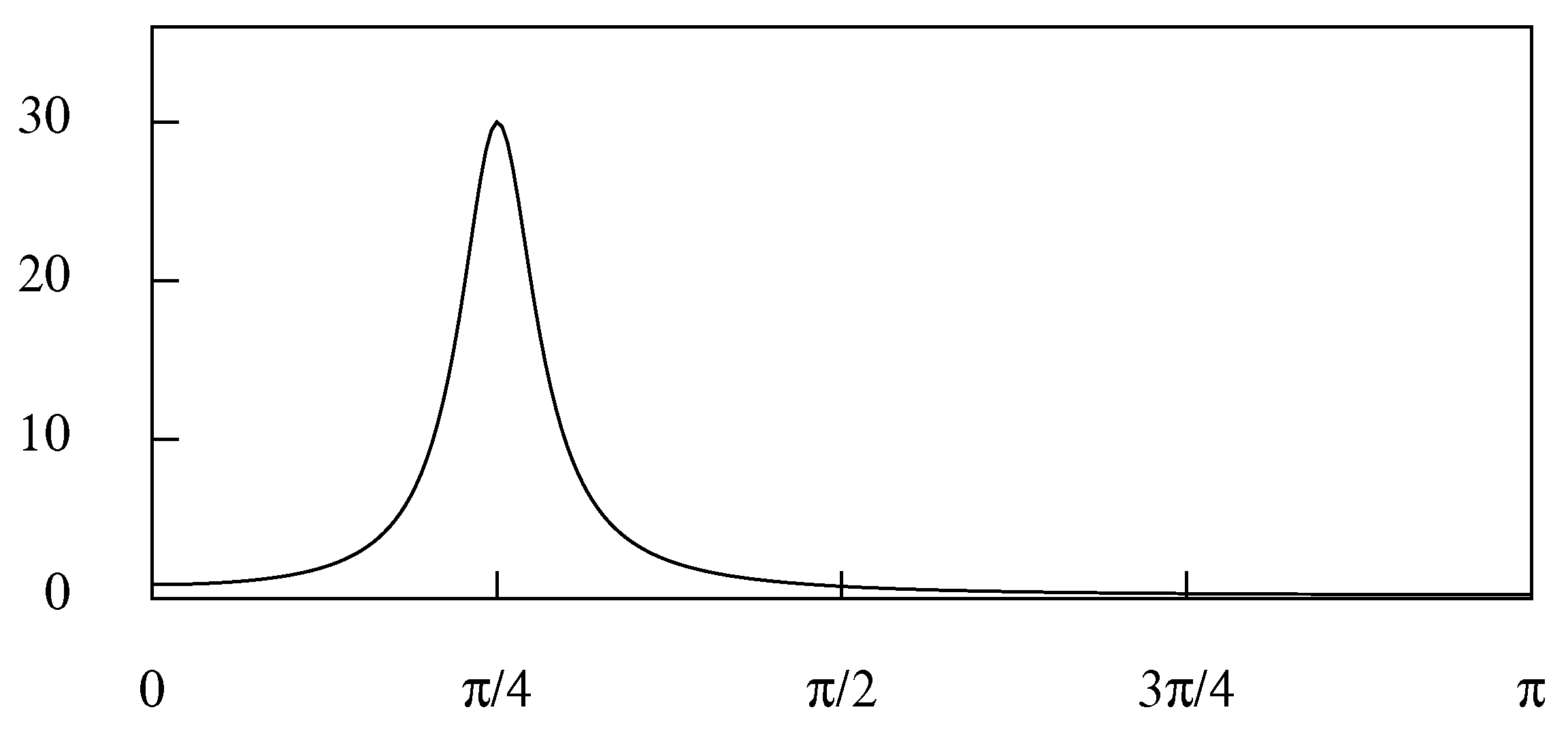
To illustrate the mapping from the discrete-time ARMA model to a continuous-time frequency-limited CARMA model, an ARMA(2, 1) model is chosen with conjugate complex poles , where and . The moving-average component has a zero of . The ARMA process generates prominent cycles of an average duration of roughly 8 periods.
The spectral density function of the ARMA process is illustrated in Figure 1. Here, it will be observed that the function is virtually zero at the limiting Nyquist frequency of π. Therefore, it is reasonable to propose that the corresponding continuous-time model should be driven by a white-noise forcing function that is bounded by the Nyquist frequency.
The parameters of the resulting continuous-time frequency-limited CARMA model are displayed below, beside those of the ARMA model:
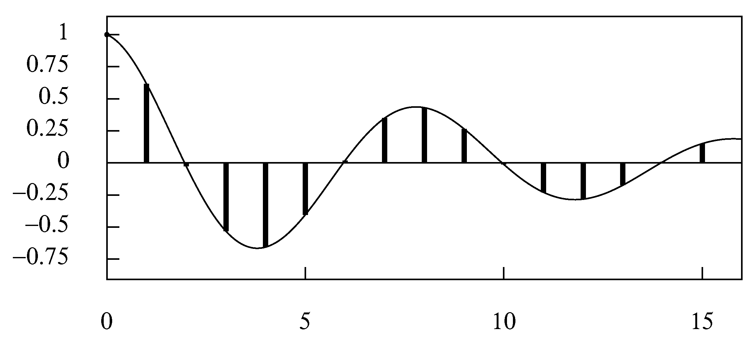
In Figure 2, the discrete autocovariance function of the ARMA process is superimposed on the continuous autocovariance function of the frequency-limited CARMA process. The former has been generated by the procedure described by the recursive Equations (34)–(36). The latter has been generated by Equation (37), wherein the index τ varies continuously.
The spectral density function of the frequency-limited CARMA process is the integral Fourier transform of the continuous autocovariance function, whereas the spectral density function of the ARMA process is the discrete Fourier transform of the autocovariance sequence. The frequency limitation of the CARMA process means that there is no aliasing in the sampling process. Therefore, the two spectra are identical within the Nyquist interval.
6.2. From ARMA to LSDE
When a linear stochastic differential equation (LSDE) is driven by a white-noise forcing function of unbounded frequencies, the ARMA model that represents its discrete-time counterpart, which is the EDLM, is bound to be affected by aliasing, even if this is to a negligible extent. The aliasing also affects the impulse response function. Therefore, the principle of impulse invariance can no longer serve to determine the parameters of the continuous-time model. Instead, the principle of autocovariance equivalence, enunciated by Bartlett (1946), must be relied upon to translate from the discrete-time model to the continuous-time model.
This principal asserts that the continuous-time autocovariance function must be equal, at the integer points, to that of the discrete-time model. Given that the autoregressive parameters of the LSDE are implied by those of the EDLM, it follows that only the moving-average parameters are liable to be determined in fulfilment of the principle.
Let be the autocovariance function of the EDLM, as given by Equation (37), and let be the corresponding autocovariance function of the LSDE, which is sampled at the integer points from the function of (40). Since Equation (60) expresses the poles of the LSDE in terms of those of the ARMA model, there is , and the principle of autocovariance equivalence can be expressed via the equation
Then, the parameters of the LSDE can be derived once a value of has been found that satisfies this equation.
The value of c can be found by using an iterative optimisation procedure to find the zero of the function
wherein are a set of positive weights. The weights should normally be set to unity, but the use of differential weights might assist the convergence of the iterations.
It will be observed that the coefficients of the continuous autocovariance function of (40) are liable to be complex-valued. This can make it tedious, if not difficult, to calculate the analytic derivatives of , which might be required by the optimisation procedure. Therefore, the derivative-free procedure of Nelder and Mead (1965) can be used to advantage. The algorithm has been coded in Pascal by Bundy and Garside (1978).
The autocovariance function of the LSDE can also be rendered in a form suggested by Equation (48), wherein the parameters are real-valued.
Söderström (1990) has determined the possible locations of the zeros of an EDLM(2, 1) as a function of the poles of the LSDE to which it corresponds; and he has shown that the zeros can only occur in a restricted set within the unit circle. This affects the possibility of finding an LSDE to correspond to a specified ARMA model.
An ingredient of the algorithm of Söderström (1991) for translating an ARMA model to an LSDE is a spectral factorisation. If the factorisation cannot be accomplished, then there is no corresponding continuous-time model. Therefore, it has been proposed that the algorithm is an appropriate means of determining whether there exists an LSDE corresponding to a specified ARMA model.
Whenever there exists a continuous-time LSDE of which the sampled autocovariance function conforms to that of an ARMA process, it is said that the ARMA process is embedded in the LSDE. Brockwell (1995) has also investigated the conditions that must be fulfilled by the ARMA process if it is to be embeddable. He has shown that every discrete-time AR(2) process with distinct complex conjugate roots can be embedded in either a continuous-time LSDE(2, 1) process or a in continuous-time LSDE(4, 2) process, or, in some cases, in both.
For the algorithm that we are pursuing, the non-availability of an LSDE corresponding to the ARMA model is indicted by a nonzero minimum of the criterion function. However, when the minimum is close to zero, then the ARMA model will be close to the EDML that corresponds to the minimising LSDE.
In such cases, we might surmise that the divergence of the ARMA model from the EDLM may be due to the vagaries of the processes of sampling and estimation that have given rise to the ARMA model. We might also surmise that the minimising LSDE will be close to one that would be delivered by a direct method of estimation applied to the sample from which the ARMA model has arisen.
Example 3.
The mapping from the discrete-time ARMA model to a continuous-time LSDE model can be illustrated, in the first instance, with the ARMA(2, 1) model of Example 2.
The parameters of the corresponding LSDE(2, 1) model are obtained by using the Nelder–Mead procedure to find the minimum of the criterion function of (63), where it is assumed that the variance of the forcing function is .
There are four points that correspond to zero-valued minima, where the ordinates of the discrete and continuous autocovariance functions coincide at the integer points. These four points, together with the corresponding moving-average parameters, are shown in Table 1.
Here, the parameter values of (i) and (iv) are equivalent, as are those of (ii) and (iii). Their difference is a change of sign, which can be eliminated by normalising at unity and by adjusting variance of the forcing function accordingly.
The miniphase condition, which corresponds to the invertibility condition of a discrete-time model, requires the zeros to be in the left half of the s-plane. Therefore, (ii) and (iii) on the NE–SW axis are the chosen pair.
These estimates of the LSDE(2, 1) are juxtaposed below with those of the frequency-limited CARMA(2, 1) model derived from the same ARMA model:
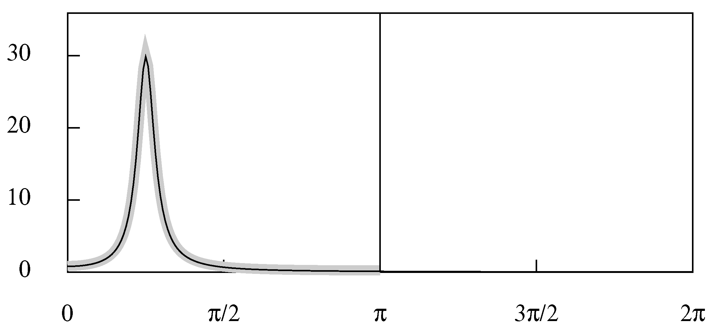
The autoregressive parameters of the frequency-limited CARMA model and of the LSDE model are, of course, identical. However, there is a surprising disparity between the two sets of moving-average parameters. Nevertheless, when they are superimposed on the same diagram—which is Figure 3—the spectra of the two models are seen virtually to coincide. Moreover, the parameters of the ARMA model can be recovered exactly from those of the LSDE by an inverse transformation, which will be described later.
The explanation for this outcome is to be found in the remarkable flatness of the criterion function in the vicinity of the minimising points, which are marked on both sides of Figure 4 by black dots. The flatness implies that a wide spectrum of the parameter values of the LSDE will give rise to almost identical autocovariance functions and spectra.
The left side of Figure 4 show the some equally-spaced contours of the z-surface of the criterion function, which are rising from an annulus that contains the minima. The minima resemble small indentations in the broad brim of a hat.
The right side of Figure 4, which is intended to provide more evidence of the nature of the criterion function in the vicinity of the minima, shows the contours of the function , where d is a small positive number that prevents a division by zero. We set , where , and where . The extended lenticular contours surrounding the minima are a testimony to the virtual equivalence of a wide spectrum of parameter values.
A variant to the ARMA(2, 1) model is one that has a pair of complex conjugate poles with the same argument as before, which is , and with a modulus that has been reduced to . The model retains the zero of the transfer function (i.e., the root of the moving-average operator) of . The ARMA parameters and those of the corresponding LSDE are as follows:
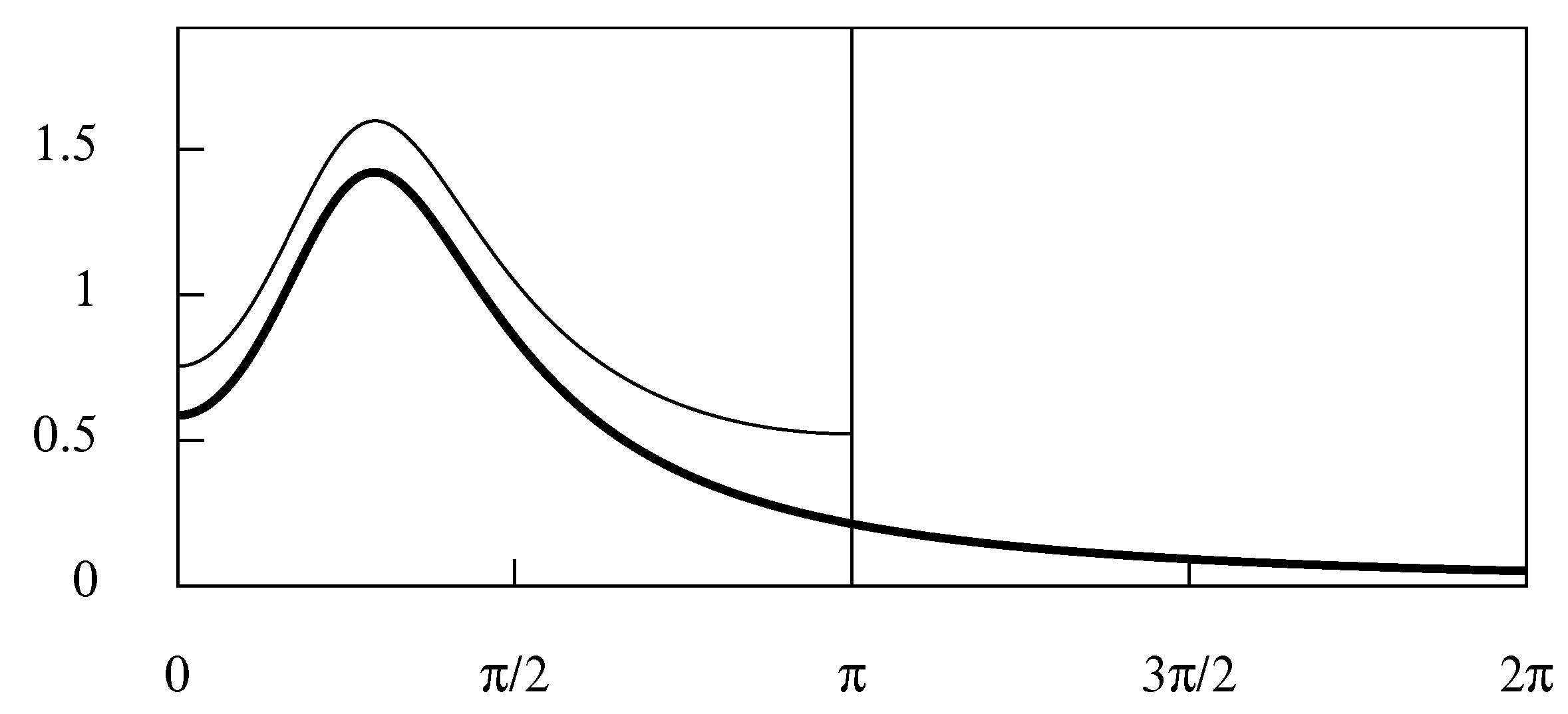
Figure 5 shows the spectral density function of the LSDE and of the ARMA model superimposed on same diagram. The spectrum of the LSDE extends far beyond the Nyquist frequency of π, which is the limiting ARMA frequency.
The ARMA process, which is to be regarded as a sampled version of the LSDE, which is the EDLM, is seen to suffer from a high degree of aliasing, whereby the spectral power of the LSDE that lies beyond the Nyquist frequency is mapped into the Nyquist interval , with the effect that the profile of the ARMA spectrum is raised considerably. On this basis, it can be asserted that the ARMA model fails to reveal the frequency content of the underlying continuous-time process. However, its other uses, such as a means of making forecasts, are unaffected.
6.3. From LSDE to ARMA
The mapping from the LSDE to the EDLM also depends on the principle of autocovariance equivalence. Thus, the ARMA parameters will be derived from the sampled ordinates the continuous-time autocovariance function of the LSDE. The essential equation is that of (31), which can be cast in the form of
where is the z-transform of the elements sampled from the autocovariance function to the LSDE.
Since the discrete-time autoregressive parameters within can be inferred from those of the LSDE, only the moving-average parameters within need to be derived from Equation (64). They can be obtained, together with the variance parameter , by a Cramér–Wold Factorisation. A Newton–Raphson algorithm for effecting the factorisation has been presented by Wilson (1969), and it has been coded in Pascal and C by Pollock (1999).
7. Summary and Conclusions
The intention of this paper has been to clarify the relationship between unconditional linear stochastic models in discrete and continuous time, and to provide a secure means of relating such models to each other.
The results of the paper emphasise the importance of an awareness of the frequency-domain characteristics of the forcing functions of such models.
In a recent paper—Pollock (2012)—the author has shown that there are liable to be severe biases in the estimated parameters of ARMA models when the data have a frequency limit significantly below the Nyquist value of , which is the maximum frequency for a discrete-time model.
A way of overcoming the problem is to create a continuous data trajectory by Fourier interpolation, from which new values can be resampled at an appropriate rate that is less than the original rate of sampling. The procedure invokes the concept of a frequency-limited continuous-time CARMA model.
The present paper further explores both the frequency-limited CARMA model and the usual linear stochastic differential equations (LSDEs) that are driven by a white-noise forcing functions of unbounded frequencies.
Example 3 shows the aliasing effects that occur when the forcing function has no frequency limit and when the ARMA transfer function imposes only a weak attenuation on the high-frequency elements. This provides a justification for adopting an LSDE of unbounded frequencies for the continuous-time translation of the ARMA model.
Given that continuous-time models are bound to be inferred from discretely sampled data, it is appropriate to base their estimation on the discrete-time autocovariance functions that are provided by ARMA models.
A secure method of translating from a discrete autocovariane function to a continuous model has been proposed. The method has been realised in the computer program CONCRETE.PAS, which is available at the author’s website, where both the compiled program and it code can be found. The program requires the prior specification on an ARMA model in the discrete-time domain, or an LSDE in the continuous-time domain. It proceeds from either of these starting points to find the corresponding model in the other domain. It is intended to develop the program by including direct maximum-likelihood methods of estimation in both the discrete and the continuous domains.
An associated program CONTEXT.PAS is also available, which plots the contour map of the surface of the criterion function that is employed in matching the autocovariance function of the LSDE to that of the ARMA model (Supplementary Materials).
As Söderström (1990, 1991), and others have noted, there are ARMA models for which there are no corresponding LSDE’s. The procedure for translating from an ARMA model to an LSDE that has been described in the present paper reveals such cases by its failure to find a zero-valued minimum of the criterion function. However, it can be relied upon to find the LSDE most closely related to the ARMA model.
One of the bugbears in estimating an LSDE is the need to satisfy the miniphase condition, by ensuring that the zeros fall on the left side of the s-plane. The way to achieve this is to find the zeros by factorising the moving-average polynomial, and then to reflect them across the vertical, imaginary, axis if they happen to fall on the right side. This is an inescapable burden whenever the order of the moving-average component is greater than one.
Supplementary Materials
The programs CONCRETE.PAS and CONTEXT.PAS are available online at https://www.le.ac.uk/users/dsgp1/ and at http://www.sigmapi.org.uk/. The following is available online at https://0-www-mdpi-com.brum.beds.ac.uk/2225-1146/8/3/35/s1, File S1: Band-Limited Stochastic Processes in Discrete and Continuous Time.
Funding
This research received no external funding.
Conflicts of Interest
The author declares no conflict of interest.
References
- Bartlett, Maurice S. 1946. On the Theoretical Specification and Sampling Properties of Autocorrelated Time Series. Supplement to the Journal of the Royal Statistical Society 8: 27–41. [Google Scholar] [CrossRef]
- Bergstrom, Albert R. 1966. Nonrecursive Models as Discrete Approximations to Systems of Stochastic Differential Equations. Econometrica 34: 173–82. [Google Scholar] [CrossRef]
- Bergstrom, Albert R. 1984. Continuous time stochastic models and issues of aggregation over time. In Handbook of Econometrics. Edited by Zvi Griliches and Michael D. Intriligator. Amsterdam: North-Holland, Volume 2, pp. 1145–212. [Google Scholar]
- Brockwell, Peter J. 1995. A Note on the Embedding Discrete-Time ARMA Processes. Journal of Time Series Analysis 16: 451–60. [Google Scholar] [CrossRef]
- Bundy, Brian D., and Gerald R. Garside. 1978. Optimisation Methods in Pascal. Baltimore: Edward Arnold. [Google Scholar]
- Chambers, Marcus J. 1999. Discrete time representation of stationary and non-stationary con-tinuous time systems. Journal of Economic Dynamics and Control 23: 619–39. [Google Scholar] [CrossRef]
- Chambers, Marcus J., and Michael A. Thornton. 2012. Discrete Time Representation of Continuous Time ARMA Processes. Econometric Theory 28: 219–38. [Google Scholar] [CrossRef] [Green Version]
- Fishman, George S. 1969. Spectral Methods in Econometrics. Cambridge: Harvard University Press. [Google Scholar]
- Granger, Clive William John, and Michio Hatanaka. 1964. Spectral Analysis of Economic Time Series. Princeton: Princeton University Press. [Google Scholar]
- Granger, Clive William John, and Paul Newbold. 1977. Forecasting Economic Time Series. New York: Academic Press. [Google Scholar]
- Harvey, Andrew C., and James Stock. 1985. The Estimation of Higher Order Continuous Time Autoregressive Models. Econometric Theory 1: 97–112. [Google Scholar] [CrossRef] [Green Version]
- Harvey, Andrew C., and James Stock. 1988. Continuous-time Autoregressive Models with Common Stochastic Trends. Journal of Economic Dynamics and Control 12: 365–84. [Google Scholar] [CrossRef]
- Hyndman, Rob J. 1993. Yule–Walker Estimates for Continuous-Time Autoregressive Models. Journal of Time Series Analysis 14: 281–96. [Google Scholar] [CrossRef]
- James, Glyn. 2004. Advanced Modern Engineering Mathematics, 3rd ed. London: Pearson Prentice Hall. [Google Scholar]
- Jones, Richard H. 1981. Fitting a Continuous Time Autoregression to Discrete Data. In Applied Time Series Analysis II. Edited by David F. Findley. New York: Academic Press, pp. 651–82. [Google Scholar]
- Larsson, Erik K., Magnus Mossberg, and Torsten Soderstrom. 2006. An Overview of Important Practical Aspects of Continuous-Time ARMA System Identification. Circuits, Systems and Signal Processing 25: 17–46. [Google Scholar] [CrossRef]
- McCrorie, J. Roderick. 2000. Deriving the Exact Discrete Analog of a Continuous Time System. Econometric Theory 16: 998–1015. [Google Scholar] [CrossRef]
- Müller, David E. 1956. A Method of Solving Algebraic Equations Using an Automatic Computer. Mathematical Tables and Other Aids to Computation (MTAC) 10: 208–15. [Google Scholar] [CrossRef]
- Nelder, John A., and Roger Mead. 1965. A Simplex Method for Function Minimization. Computer Journal 7: 308–13. [Google Scholar] [CrossRef]
- Nyquist, Harry. 1924. Certain Factors Affecting Telegraph Speed. Bell System Technical Journal 3: 324–46. [Google Scholar] [CrossRef]
- Nyquist, Harry. 1928. Certain Topics in Telegraph Transmission Theory. Transactions of the AIEE 47: 617–44, Reprinted in 2002, Proceedings of the IEEE 90: 280–305. [Google Scholar] [CrossRef]
- Oppenheim, Alan V., and R. W. Schafer. 2013. Discrete-Time Signal Processing. Englewood Cliffs: Prentic-Hall. [Google Scholar]
- Pollock, David Stephen Geoffrey. 1999. A Handbook of Time-Series Analysis, Signal Processing and Dynamics. London: Academic Press. [Google Scholar]
- Pollock, David Stephen Geoffrey. 2009. Realisations of Finite-sample Frequency-selective Filters. Journal of Statistical Planning and Inference 139: 1541–58. [Google Scholar] [CrossRef] [Green Version]
- Pollock, David Stephen Geoffrey. 2012. Band-Limited Stochastic Processes in Discrete and Continuous Time. Studies in Nonlinear Dynamics and Econometrics 16: 1–37. [Google Scholar] [CrossRef] [Green Version]
- Pollock, David Stephen Geoffrey. 2015. Econometric Filters. Computational Economics 48: 669–91. [Google Scholar] [CrossRef]
- Pollock, David Stephen Geoffrey. 2018. Filters, Waves and Spectra. Econometrics 6: 35. [Google Scholar] [CrossRef] [Green Version]
- Priestley, M.B. 1981. Spectral Analysis and Time Series. London: Academic Press. [Google Scholar]
- Shannon, Claude Elwood. 1949. Communication in the Presence of Noise. Proceedings of the Institute of Radio Engineers 37: 10–21, Reprinted in 1998, Proceedings of the IEEE 86: 447–57. [Google Scholar]
- Söderström, T. 1990. On Zero Locations for Sampled Stochastic Systems. IEEE Transactions on Automatic Control 35: 1249–53. [Google Scholar] [CrossRef]
- Söderström, T. 1991. Computing Stochastic Continuous-Time Models from ARMA Models. International Journal of Control 53: 1311–26. [Google Scholar] [CrossRef]
- Wilson, G. T. 1969. Factorisation of the Covariance Generating Function of a Pure Moving Average Process. SIAM Journal of Numerical Analysis 6: 1–7. [Google Scholar] [CrossRef]
Figure 1.
The spectrum of the ARMA(2, 1) process .

Figure 2.
The discrete autocovariance sequence of the ARMA(2, 1) process and the continuous autocovariance function of the corresponding frequency-limited CARMA(2, 1) process.
Figure 2.
The discrete autocovariance sequence of the ARMA(2, 1) process and the continuous autocovariance function of the corresponding frequency-limited CARMA(2, 1) process.

Figure 3.
The spectrum of the LSDE(2, 1) corresponding to the ARMA(2, 1) model of Example 1 plotted on top of the spectrum of that model, represented by the thick grey line. The two spectra virtually coincide over the interval .
Figure 3.
The spectrum of the LSDE(2, 1) corresponding to the ARMA(2, 1) model of Example 1 plotted on top of the spectrum of that model, represented by the thick grey line. The two spectra virtually coincide over the interval .

Figure 4.
(Left) The contours of the criterion function together with the minimising values, marked by black dots. (Right) The contours of the function .
Figure 4.
(Left) The contours of the criterion function together with the minimising values, marked by black dots. (Right) The contours of the function .
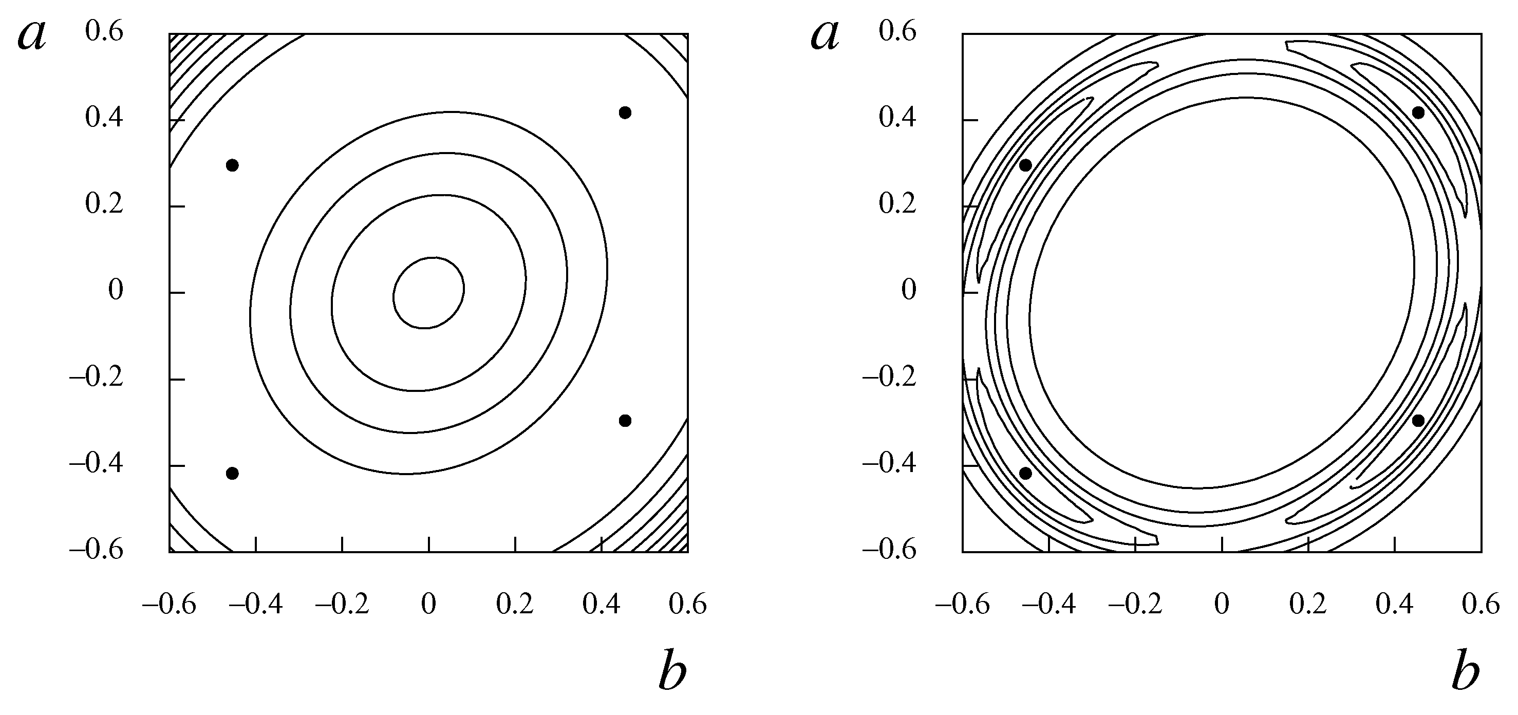
Figure 5.
The spectrum of the revised ARMA model, confined to the interval , superimposed on the spectrum of the derived LSDE—the bold line.
Figure 5.
The spectrum of the revised ARMA model, confined to the interval , superimposed on the spectrum of the derived LSDE—the bold line.


Table 1.
The various values to the moving-average parameters of the LSDE(2, 1) model inferred from the discrete-time autocovariance function according to the principle of autocovariance equivalence. The parameters a and b are arguments of the continuous autocovariance function of (48).
Table 1.
The various values to the moving-average parameters of the LSDE(2, 1) model inferred from the discrete-time autocovariance function according to the principle of autocovariance equivalence. The parameters a and b are arguments of the continuous autocovariance function of (48).
| a | b | |||
|---|---|---|---|---|
| (i) | −0.4544 | 0.2956 | −0.9088 | 0.5601 |
| (ii) | 0.4544 | 0.4175 | 0.9088 | 0.5601 |
| (iii) | −0.4544 | −0.4174 | −0.9088 | −0.5601 |
| (iv) | 0.4544 | −0.2956 | 0.9088 | −0.5601 |
© 2020 by the author. Licensee MDPI, Basel, Switzerland. This article is an open access article distributed under the terms and conditions of the Creative Commons Attribution (CC BY) license (http://creativecommons.org/licenses/by/4.0/).
Share and Cite
MDPI and ACS Style
Pollock, D.S.G. Linear Stochastic Models in Discrete and Continuous Time. Econometrics 2020, 8, 35. https://0-doi-org.brum.beds.ac.uk/10.3390/econometrics8030035
AMA Style
Pollock DSG. Linear Stochastic Models in Discrete and Continuous Time. Econometrics. 2020; 8(3):35. https://0-doi-org.brum.beds.ac.uk/10.3390/econometrics8030035
Chicago/Turabian StylePollock, D. Stephen G. 2020. "Linear Stochastic Models in Discrete and Continuous Time" Econometrics 8, no. 3: 35. https://0-doi-org.brum.beds.ac.uk/10.3390/econometrics8030035
Note that from the first issue of 2016, this journal uses article numbers instead of page numbers. See further details here.