Long-Lasting Economic Effects of Pandemics:Evidence on Growth and Unemployment

Abstract

This paper studies long economic series to assess the long-lasting effects of pandemics. We analyze if periods that cover pandemics have a change in trend and persistence in growth, and in level and persistence in unemployment. We find that there is an upward trend in the persistence level of growth across centuries. In particular, shocks originated by pandemics in recent times seem to have a permanent effect on growth. Moreover, our results show that the unemployment rate increases and becomes more persistent after a pandemic. In this regard, our findings support the design and implementation of timely counter-cyclical policies to soften the shock of the pandemic.

1. Introduction

The COVID-19 pandemic has already cost the lives of hundreds of thousands of people around the globe. COVID-19 can be positioned as one of the worst pandemics in history (see Ferguson et al. 2020). They estimate the death toll at 510,000 only in Britain. This incommensurable cost to human society is accompanied by an intense economic shock. As COVID-19 spreads through the globe, countries started to impose restrictions on economic activity to slow the rate of infection. The early economic results following the start of the pandemic, and considering possible new waves of infections, point to a deep recession and the loss of millions of jobs (see Colbourn 2020; Prem et al. 2020). Moreover, even though some countries have started to relax some of the restrictions, the consensus is that overall economic activity will not rapidly return to levels achieved before the pandemic (see, e.g., Guerrieri et al. 2020; McKibbin and Fernando 2020). In this context, this paper uses long economic series to gather lessons from history for the post-pandemic world.

Pandemics are random, infrequent events. We require long datasets spanning several centuries to study them properly. Thus, we focus on data from the United Kingdom (UK, henceforth), given the existence of long series encompassing several centuries. The vast amount of data allows us to study the effect of previous pandemics on both growth and unemployment. We consider the deadliest episodes in the history of the UK in terms of total estimates of deaths.

Table 1. Main outbreaks and pandemics in terms of death toll in the UK the respective period. Source: https://en.wikipedia.org/wiki/List_of_epidemics and references therein. ${}^{*}$ The death toll in London alone is estimated to have been of up to 20%.

Period	Outbreaks or Pandemics	Death Toll in the UK	Death Rate in the UK
1270–1350	Black Death	Between 112,000 and 270,000	Between 25% and 60%
1427–1580	Small London plagues	≈40,000	≈2%
1581–1644	Small London plagues	≈50,000	≈1.5%
1645–1705	Great Plague of London ${}^{*}$	>100,000	>2%
1834–1920	Different cholera outbreaks,	≈160,000	≈1.5%
	Great Pandemic of 1870–1875,	≈80,000	≈0.5%
	and Russian flu	>100,000	>0.5%
1921–2019	Spanish flu and remaining	≈228,000	≈1%
	pandemics of the 20th century

shows the relevant outbreaks and pandemics in each period.

As documented by many historians, the most devastating pandemic has been the Black Death. Due to the lack of historical record in that time, it is extremely difficult to establish the death toll with a satisfactory degree of certainty. Even today, many historians still debate it, although a consensus estimates that the death toll is around 25–60% of the total population only in the UK. This pandemic was also relevant in terms of economic, social, and political change in Europe, particularly in England (see Clark 2007, 2010; Jordà et al. 2020). After the Black Death, small plagues were frequent in England in the next three centuries. Another relevant pandemic in the UK was the Great Plague of London; it is considered the last major epidemic of the bubonic plague to occur in England with a considerable number of deaths. With the increase in population, outbreaks and pandemics have been more devastating after the 18th century. The worst pandemic in terms of loss of human life is the Spanish flu, which originated alongside the First World War.

Several studies have focused on the short-term economic consequences of different outbreaks and pandemics (see, e.g., Brainerd and Siegler 2003; Karlsson et al. 2014; Meltzer et al. 1999). Until recently, there has been an increase in interest in studying the medium- and long-term economic impacts of global pandemics (see Jordà et al. 2020; Prados de la Escosura and Rodríguez-Caballero 2020). This paper adds to this line of research using econometric techniques that, to the best of our knowledge, have not been explored before to study the possible long-lasting effects of epidemics in the economy.

Given the size of the economic shocks, it is of the utmost importance to determine the possible long-lasting effects of the pandemics. Long memory is the statistical property that events in the past can be felt even after much time has passed—that is, events are more persistent than what standard models are capable of capturing. Establishing the long memory properties of an economic series helps in understanding the long-lasting effects of shocks. While the impact of shocks is transitory for stationary series, random shocks have permanent effects for nonstationary cases. In this regard, if an economic series has long memory properties, we can expect calamities to affect the economy for the considerable future. Thus, the assessment of the level of persistence that pandemics have on the economy is of major interest in light of the current COVID-19 pandemic. If the effects of the pandemic are short memory, not showing a high level of persistence, we could expect a rapid recovery after the current crisis—that is, a V-shaped recovery. If, on the other hand, the effects of the pandemic are persistent, we could expect a slow U-shaped recovery.

Thus, this paper gathers evidence from previous periods that cover pandemics to determine their long memory properties and provide more information to help in the recovery post-COVID-19. The statistical analysis in this paper is designed to test if shocks that occurred inside regimes associated with a pandemic are more persistent compared to those periods without notable pandemics. Even if analyzing actual causal effects running from pandemics to the general performance of an economy is an urgent issue given the contemporaneous global health situation, due to data limitations in historical pandemics, it remains beyond the scope of the present research.

This paper is organized as follows. The next section introduces the econometric tools used in the paper. In Section 3, we study the persistence levels in periods with outbreaks and epidemics in the UK for real GDP per capita and unemployment. Section 4 extends the analysis on growth to other countries with long economic series: Spain, Italy, the Netherlands, and the USA. Finally, Section 5 presents some concluding remarks and policy recommendations.

2. Structural Changes and Long Memory

This section presents the econometric tools that we will use to assess the long-lasting effects of outbreaks and pandemics in the economy. We present the fractional difference operator, the most used procedure to model long memory in the econometric literature, and semiparametric methods to estimate the long memory parameter. Moreover, we present tests for structural change in levels and trends, and changes in persistence.

2.1. Tests for Structural Breaks

The method proposed by Bai and Perron (1998, 2003) (BP, henceforth) deals with multiple unknown breaks, making the methodology suitable for a broad range of applications.

The general framework of BP analysis can be described by the following multiple linear regression model with b breaks, that is $b+1$ periods or regimes,

$$y_t=x_t\beta +z_t{\delta }_j+u_t,t=T_{j-1}+1,\cdots ,T_j,$$

(1)

for $j=1,\cdots ,b+1$, where $y_t$ is the dependent variable at time t, $x_t$ and $z_t$ are vectors of covariates with $\beta$ and ${\delta }_j(j=1,\cdots ,b+1)$ their corresponding vector of coefficients, and $u_t$ is the usual disturbance at time t. Since the method treats the breakpoint indices, $1<T_1<\cdots <T_b<T$, as unknown, the goal is the joint estimation of the unknown parameters together with the breakpoints.

The BP methodology employs a sequential F-test to infer the number of shifts on a time series. The idea is that the full sample is divided into subsamples. The null hypothesis is stability in the regression coefficients between subsamples, while the alternative considers that at least one of the parameters varies over time. Bai and Perron (1998) computes the asymptotic critical values up to nine breaks via simulations.

It is worthwhile to note that the BP methodology tests for changes in regimes but does not assess causality—that is, the BP methodology estimates dates when the series shows structural changes, but it does not identify the generating mechanism behind them. In this regard, we treat the results form the BP methodology as evidence that a structural change has occurred, and we point to the state of the economy in each regime in terms of the occurrence of pandemics. We then test if shocks that originated in periods associated with a pandemic are more persistent than shocks in periods where no major pandemics are reported as a test for the long-lasting effects of pandemics.

2.2. The Fractional Difference Operator

The most common procedure to model long-lasting effects or long memory is the fractional difference operator of Granger and Joyeux (1980) and Hosking (1981). The authors proposed to model a time series, $x_t$, as:

$$x_t={(1-L)}^d{\epsilon }_t,$$

(2)

where $L(·)$ is the lag operator such that $L\left(x_t\right)=x_{t-1}$, ${\epsilon }_t$ is a white noise process with variance ${\sigma }^2$, and $d\in (-1/2,3/2)$. Following the standard binomial expansion, the fractional difference operator, ${(1-L)}^d$, is decomposed to generate a series given by:

$$x_t=\sum _{k=0}^{\infty }{\pi }_k{\epsilon }_{t-k},$$

(3)

with coefficients ${\pi }_k=\Gamma (k+d)/[\Gamma \left(d\right)\Gamma (k+1)]$ for $k\in \mathbb{N}$, where $\Gamma (·)$ is the standard gamma function.

The properties of the fractional difference operator have been well documented in, among others, Beran et al. (2013). We note the following implications of the parameter d:

• A process with $d=0$ displays short memory and implies that any shock that affects the series only has repercussions in the short term. Thus, its impact will completely vanish in the long run.
• The process will display long memory for $0<d<1$, and implies that any shock that affects the series has long-lasting repercussions.
• The process will be stationary as long as $d<1/2$.
• The process will revert to its mean as long as $d<1$, but the speed to which it converges could be quite slow.
• Processes with $d>1$ are such that past innovations have permanent effects.

To get a better understanding of the long memory properties of fractionally differenced processes,

Table 2. Number of lags for the autocorrelation function to fall below the given threshold value.

Memory	Autocorrelation Threshold
$\mathbf{d}$	${\mathbf{10}}^{-\mathbf{1}}$	${\mathbf{10}}^{-\mathbf{2}}$	${\mathbf{10}}^{-\mathbf{3}}$	${\mathbf{10}}^{-\mathbf{4}}$
0.1	3	22	367	>500
0.2	6	220	>500	>500
0.3	41	>500	>500	>500
>0.4	>500	>500	>500	>500

shows the number of lags necessary for the autocorrelations to fall below specific values approaching zero. The table shows that as the d parameter increases, it takes more lags for the autocorrelations to fall below every threshold. In particular, notice that it takes more than 500 lags for the autocorrelations of a fractionally differenced process with parameter $0.4$ to fall below 0.1, showing the long memory properties of the process. That is, the effects of a shock that occurs in a long memory process are significant even after many periods have passed.

Furthermore, let $f_X\left(\lambda \right)$ be the spectral density at frequency $\lambda \in \mathbb{R}$ of a fractionally differenced process, then:

$$f_X\left(\lambda \right)=\frac{{\sigma }^2}{2\pi }{\left|\sum _{k=0}^{\infty }{\pi }_k{e}^{-ik\lambda }\right|}^2=\frac{{\sigma }^2}{2\pi }{\left|1-e^{-i\lambda }\right|}^{-2d}\sim \frac{{\sigma }^2}{2\pi }{\lambda }^{-2d}\mathrm{as}\lambda \to 0,$$

(4)

where $i^2=-1$, ${\pi }_k$ are given in Equation (3), and where we use the notation $f\left(k\right)\sim g\left(k\right)$ as $k\to k_0$ to denote that ${lim}_{k\to k_0}f\left(k\right)/g\left(k\right)=1$.

Fractionally integrated models have been extensively used in empirical applications. For instance, Gil-Alana and Robinson (1997) analyze whether the macroeconomic variables involved in the original database of Nelson and Plosser (1982), GDP and unemployment among them, have long memory. Moreover, they have been used to model asset returns, exchange rates, and electricity prices; a few recent examples can be found in Varneskov and Perron (2018); Osterrieder et al. (2019), and Ergemen et al. (2016).

2.3. Semiparametric Estimators of Long Memory

Tests for long memory include the log-periodogram regression (see Geweke and Porter-Hudak 1983; Robinson 1995) and the exact local Whittle approach of Shimotsu and Phillips (2005) that consistently estimate d beyond the unit root case. The idea is to evaluate the periodogram of the time series, an estimator of the spectral density, only in a vicinity of the origin, where the spectral density, $f_X\left(\lambda \right)$, is driven only by the memory parameter d, see Equation (4).

The log-periodogram regression [GPH, henceforth] is given by:

$$log\left(I\left({\lambda }_k\right)\right)=c-2dlog\left({\lambda }_k\right)+u_k,k=1,\cdots ,m,$$

where $I\left({\lambda }_k\right)$ is the periodogram of $x_t$, ${\lambda }_k=e^{i2\pi k/T}$ are the Fourier frequencies, c is a constant, $u_k$ is the error term, and m is a bandwidth parameter that grows with the sample size. For our analysis, we use the mean-squared error optimal bandwidth of $T^{4/5}$, where T is the sample size, obtained by Hurvich et al. (1998).

On the other hand, the exact local Whittle estimator (ELW, henceforth) minimizes the function:

$$R\left(d\right)=log\left(\frac{1}{m}\sum _{k=1}^m{I}_{{\Delta }^d}\left({\lambda }_k\right)\right)-\frac{2d}{m}\sum _{k=1}^{m}log\left({\lambda }_k\right),$$

where $I_{{\Delta }^d}\left({\lambda }_k\right)$ is the periodogram of ${(1-L)}^d{x}_t$, ${\lambda }_k=e^{i2\pi k/T}$ are the Fourier frequencies, and m is the bandwidth parameter that grows with the sample size.

From Equation (4), note that the log periodogram regression provides an estimate of the long memory parameter for fractionally differenced processes.

2.4. Tests for Change in Persistence

In recent years, several tests have been proposed to assess whether macroeconomic variables display changes in persistence within a specific period. Martins and Rodrigues (2014) (MR, henceforth) propose a test capable of detecting changes in the order of integration of a fractionally integrated process. The authors propose a method based on recursive forward and reverse estimation of the Breitung and Hassler (2002) test. The method is capable of dealing with unknown date of the change, trends, and serial correlation.

Let $x_t$ be given as in Equation (2), and let $\tau \in [{\Lambda }_l,{\Lambda }_u]$ with $1<{\Lambda }_l<{\Lambda }_U<T$, and T the sample size. To ease notation, we assume that the time series starts at $t=1$ and thus T denotes both the last observation and the sample size. The test proceeds by recursively considering the auxiliary regression given by:

$$z_t=\varphi \left(\tau \right)z_{t-1}^{*}+e_t,t=2,\cdots ,\left[\tau T\right],$$

where $z_t={(1-L)}^{-d}{x}_t$, and $z_{t-1}^{*}={\sum }_{j=1}^{t-1}{j}^{-1}{x}_{t-j}$. Intuitively, the j coefficient helps in controlling for the characteristic hyperbolic decay of long memory processes. The statistic of the test is constructed by the supreme of the squares of the t-statistics associated to $\varphi \left(\tau \right)$ as we recursively move $\tau$, and the analogous t-statistic associated to the auxiliary regression in the time-reversed rest of the series.

3. Evidence from the United Kingdom

This section presents the data used to assess the long-lasting effects of periods that have covered pandemics on the economy, particularly in growth and unemployment. We use data from the United Kingdom given the availability of large datasets spanning several centuries.

3.1. Data

We are interested in analyzing the effect that global pandemics may have had in the economy to get a preliminary assessment of the impact of the outbreak caused by the new coronavirus SARS-CoV-2. We focus on two of the most important macroeconomic variables: (i) annual real GDP per capita of the UK from 1270 to 2019, and (ii) unemployment monthly rate of the UK from July 1854 to December 2016.

For the first variable, the literature uses data provided by Conference Board (2020) and Maddison Project of Bolt et al. (2018). The standard strategy to construct the series for the UK is as follows. The Bank of England provides the series from 1870 to 2019 considering the current definition of The United Kingdom of Great Britain and Northern Ireland. A previous block of this series is obtained from 1700 to 1869 using the estimates from Broadberry et al. (2015), who reconstruct GDP from the output side for medieval and early modern Britain. The reconstruction aggregates the three main sectors of the economy in that epoch: agriculture, industry, and services.

For the second variable, we use the dataset from Thomas and Dimsdale (2017), which contains information for the UK for dozens of variables for several centuries. The dataset is available at the Bank of England data repository.

These large datasets allow us to study the long-run behavior of critical economic variables, and the effect that major outbreaks and pandemics have had on them.

3.2. Real GDP Per Capita in the UK

Here we focus on the longer time series, real GDP per capita, to analyze the persistence of different regimes, whose periods cover some relevant outbreaks and pandemics in history.

We consider a linear trend in Equation (1) as follows:

$$GDPp{c}_t={\beta }_{0,j}+{\beta }_{1,j}t+u_t,$$

(5)

for $t=T_{j-1},\dots ,T_j$, where $j=1,\dots ,b+1$ indicates the period, and t is the time index. In Equation (5), $GDPpc$ is the real GDP per capita for the UK; ${\beta }_{0,j}$, and ${\beta }_{1,j}$ are the intercept and the slope of each linear regression fitted in period j; and $u_t$ is a potentially fractionally differenced, random process. Then, the underlying idea to define a period is that either of the parameters (${\beta }_0$, and ${\beta }_1$) vary in two consecutive periods calibrated by a trimming parameter.

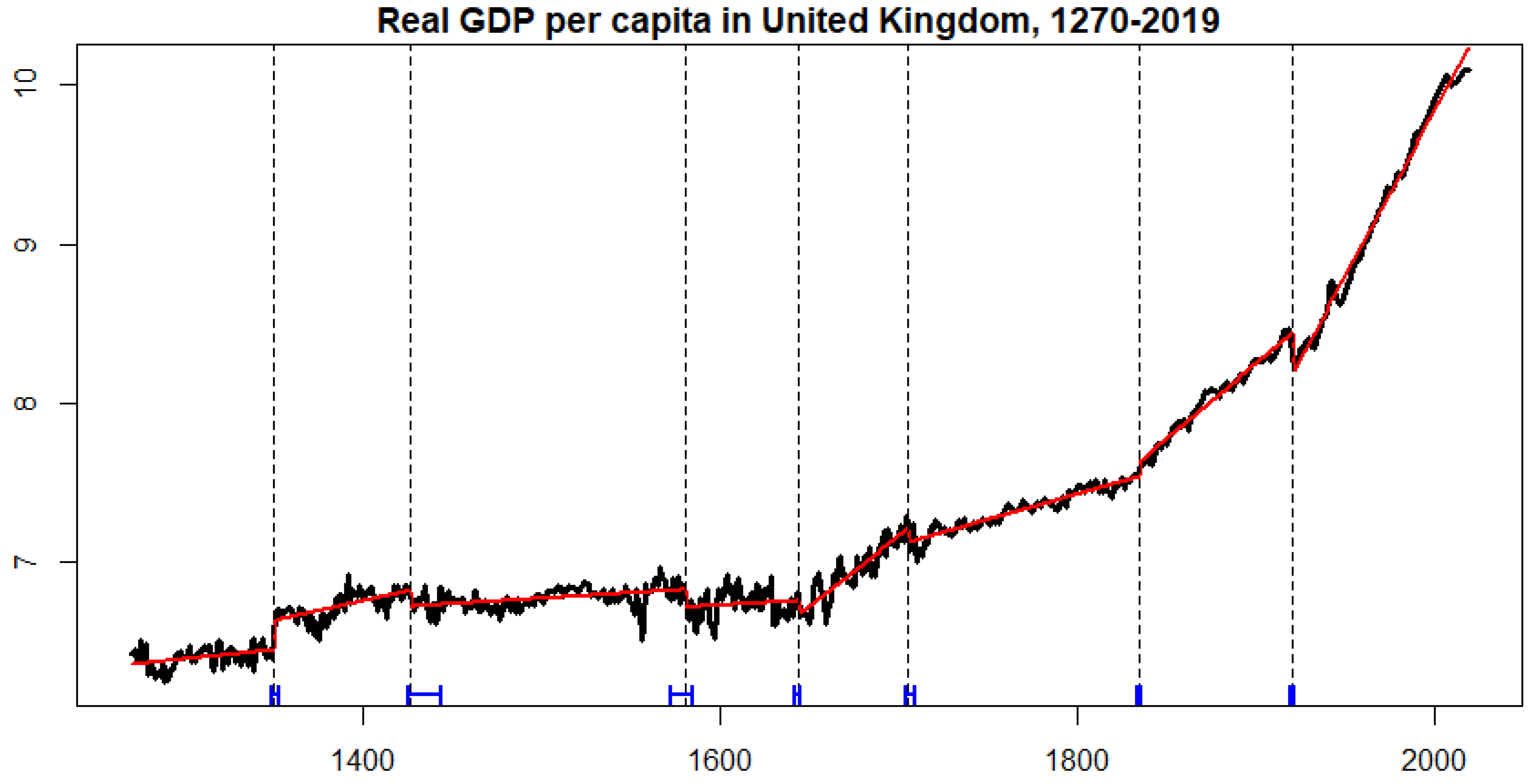
We work with the annual series of the real GDP per capita from 1270 to 2019. Figure 1 displays the respective time series, the break estimated by the BP methodology, and their confidence intervals at 95% (also presented in

Table 3. Dates for structural changes detected by the BP methodology in yearly UK real GDP per capita. The confidence intervals are shown below each date.

Estimated date		1350	1426	1580	1644
Confidence interval		[1349–1353]	[1425–1444]	[1572–1584]	[1642–1645]
Estimated date cont.		1705	1834	1920
Confidence interval cont.		[1704–1709]	[1833–1835]	[1919–1921]

).

As we can see in Figure 1, the BP methodology identifies eight periods over the last seven centuries in which GDP per capita of the United Kingdom undergoes structural changes in the aforementioned linear trend. To analyze the possible impact of COVID-19 within the current regime of the GDP per capita, firstly, it is relevant to identify the main outbreaks and pandemics along these centuries.

As seen in Table 1, we can locate outbreaks and pandemics in some of the periods defined. We consider the regimes defined by the breaks estimated in Table 3, and we estimate the respective persistence level of the random component for each period by the GPH and ELW methods explained before. The analysis is also accompanied by the MR test results to assess if there is a significant change in persistence between consecutive periods.

Table 4. Long memory estimates and change of persistence tests for yearly real GDP per capita for the UK. The table presents the estimates by both GPH and ELW methods together with their standard errors. Moreover, it presents the critical values for the MR test for the 90%, 95%, and 99% confidence levels, and the associated MR statistic for the test for change in persistence on either direction from the regime in the row above to the current row.

Period	GPH est.	GPH s.e.	ELW est.	ELW s.e.	MR Test
					90%	95%	99%	Stat.
1270–1350	0.466	0.144	0.507	0.086
1351–1426	0.597	0.147	0.583	0.087	5.324	6.440	8.878	3.122
1427–1580	0.498	0.102	0.494	0.066	5.294	6.519	9.426	2.107
1581–1644	0.589	0.161	0.606	0.093	5.288	6.497	9.335	5.155
1645–1705	0.865	0.166	0.867	0.094	5.340	6.411	8.654	5.318
1706–1834	0.877	0.112	0.813	0.071	5.331	6.495	9.139	5.653
1834–1920	1.084	0.138	1.080	0.083	5.248	6.460	9.305	11.116
1921–2019	1.041	0.129	1.186	0.079	5.690	7.022	10.853	7.846

presents the results and reveals some interesting findings.

First, there seems to be an increasing trend in the level of persistence through the regimes considered. However, we note a slight increase in persistence from the period finalizing with the Black Death pandemic to the next period that is not maintained to the subsequent period (where no major outbreak or pandemic is reported)—that is, the period after the Black Death pandemic seems to be more persistent than contiguous periods, pointing to the possible long-lasting effects of the pandemic on growth. Nonetheless, this increase in persistence does not appear to be statistically significant. The test for change in persistence does not reject the null of no change in persistence through the periods around the Black Death pandemic. One reason behind this result may be the short and imprecise data available before the pandemic.

Second, any shock before the 19th century has a non-permanent effect on the series, indicating that shocks originated from these outbreaks and epidemics were transitory even though potentially long-lasting. Moreover, we find that the small increases in persistence across the first five regimes are not statistically significant.

Third, shocks after the 19th century seem to have a permanent effect on the series, indicating that the most current outbreaks and epidemics have a longer-lasting effect on the GDP per capita. This could point to the fact that the world has become much more socially and economically connected in the last couple of centuries. Commerce and travel between countries are much more widespread, and thus the effects of global pandemics on growth are compounded. It is interesting to remark that persistence has statistically changed at 5% (at least) in the last three regimes. This gives us an idea that COVID-19 may present a change in the persistence of growth, which needs to be controlled by the policymakers.

These results highlight the relevance that the 21st century epidemics may have in the economy. It is too early to determine the persistence level of the COVID-19 pandemic on growth. Nonetheless, if the upward trend on the level of persistence of the effects of pandemics in growth is maintained, we would expect the effects of the COVID-19 pandemic to be long-lasting.

Assessing the impact of extreme events as pandemics from time series data is a big issue today. A classical perspective is conducted by a before-and-after comparison using a difference-in-difference approach. In a series of influential papers, Abadie et al. (2010), and Abadie et al. (2015) have introduced data-driven synthetic control groups by fitting multivariate time series models. On the other hand, Harvey and Thiele (2017) propose an auxiliary approach to assess the effect of an intervention or external shock from a time series perspective. However, given data limitations, it is not possible to follow these routes. In particular, by construction, there is only one real GDP per capita for the UK; and to the best of our knowledge, there is no yearly time series of confirmed cases and deaths from previous pandemics. Nevertheless, we design a pure time series analysis below to shed light on the impact of a pandemic in the economy. Once more data from the current pandemic is collected, a more conscientious analysis could be executed to deepen in this issue, but it remains out of the scope of the present paper.

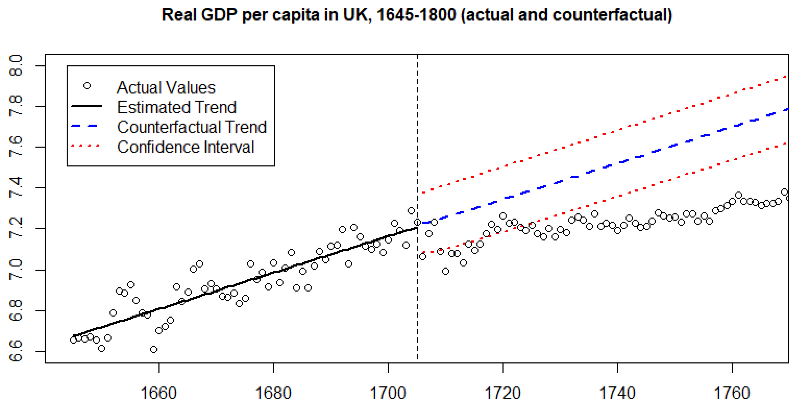
To get a better understanding of the distinct behavior of real GDP between periods with pandemics and those without them, Figure 2 presents an experiment using real GDP per capita in the UK between 1640 and 1800. The figure shows real GDP in the UK in the period associated with the Great Plague of London and the subsequent period. Moreover, we estimate the linear trend model with fractionally differenced disturbances, Equation (5), in the period associated with the pandemic, and we use it to construct the counterfactual for the subsequent period. The periods were selected given that the Great Plague of London was a more localized event (see Section 4), and that the pandemic occurred before the industrial revolution. Given our data, these two conditions allow us to study the change in trend and persistence when the international feedback loops were less pronounced. Moreover, the use of the fractional difference operator to forecast long memory processes is supported by the results of Vera-Valdés (2020). The author showed that fractionally differenced models are good at forecasting long memory processes regardless of the long memory generating mechanism.

Figure 2 allows us to compare the counterfactual behavior of real GDP in the UK under the no-break scenario against the actual values. The figure shows that the loss in real GDP was quite significant and lasted for almost a century. The average annual loss in GDP from the counterfactual to the actual values is 6%, with a maximum estimated decrease of 11%.

It is worth pointing out that we cannot directly extrapolate the results from the thought experiment in Figure 2 to the current pandemic. The world is much more connected now, which allows the virus to spread fast instead of slowly developing waves, and both the economic and medical sciences have significantly advanced in the last two centuries, which allows for a more competent response. As a prime example, large randomized control trials for a vaccine are already in motion in record time, less than a year since the virus was discovered. In this sense, these results can only be considered as a lower bound. Nonetheless, the results are instructive in the sense that they point to a long post-pandemic recovery period in the absence of economic policies designed to soften the shock of the pandemic, as was the case in the 18th century.

Furthermore, as a robustness exercise, we analyze the yearly real GDP per capita for England from the Thomas and Dimsdale (2017) dataset. Results, available upon request, corroborate the upward increasing trend in persistence across the centuries and the slightly larger persistence after the Black Death pandemic. Moreover, we used other bandwidths for the long memory estimators obtaining qualitatively similar results.

Finally, Section 4 considers growth data in Spain, Italy, the Netherlands, and the USA to show that the findings for the UK case can be extended to other countries. Thus, our results confirm that the long-lasting effects on growth are international and not restricted to a particular country.

One caveat of the above analysis is that the low sampling of the data makes it difficult to properly disentangle the impact of, for example, the Spanish flu pandemic in the economy of the United Kingdom. Periods with major pandemics are sometimes accompanied by episodes of turmoil as the First and Second World Wars, or the Great Depression. In this respect, in the next section we use a series sampled more frequently to explore further the role that epidemics may play in the economy.

3.3. Unemployment in the UK

In this section, we focus on the monthly UK unemployment rate from July 1854 to December 2016. The more frequent sampling period allows us to disentangle better the economic effects that previous pandemics had in the economy.

To model structural change in unemployment, given that a linear trend is not observed, we consider a mean-shifting specification in Equation (1) as follows:

$$U_t={\beta }_{0,j}+u_t,$$

(6)

for $t=T_{j-1},\dots ,T_j$, where $j=1,\dots ,b+1$ indicates the period, and t is time index. In Equation (6), $U_t$ is the unemployment rate for the UK; ${\beta }_{0,j}$ are the intercept of each linear regression fitted in period j; and $u_t$ is a, potentially fractionally differenced, random process.

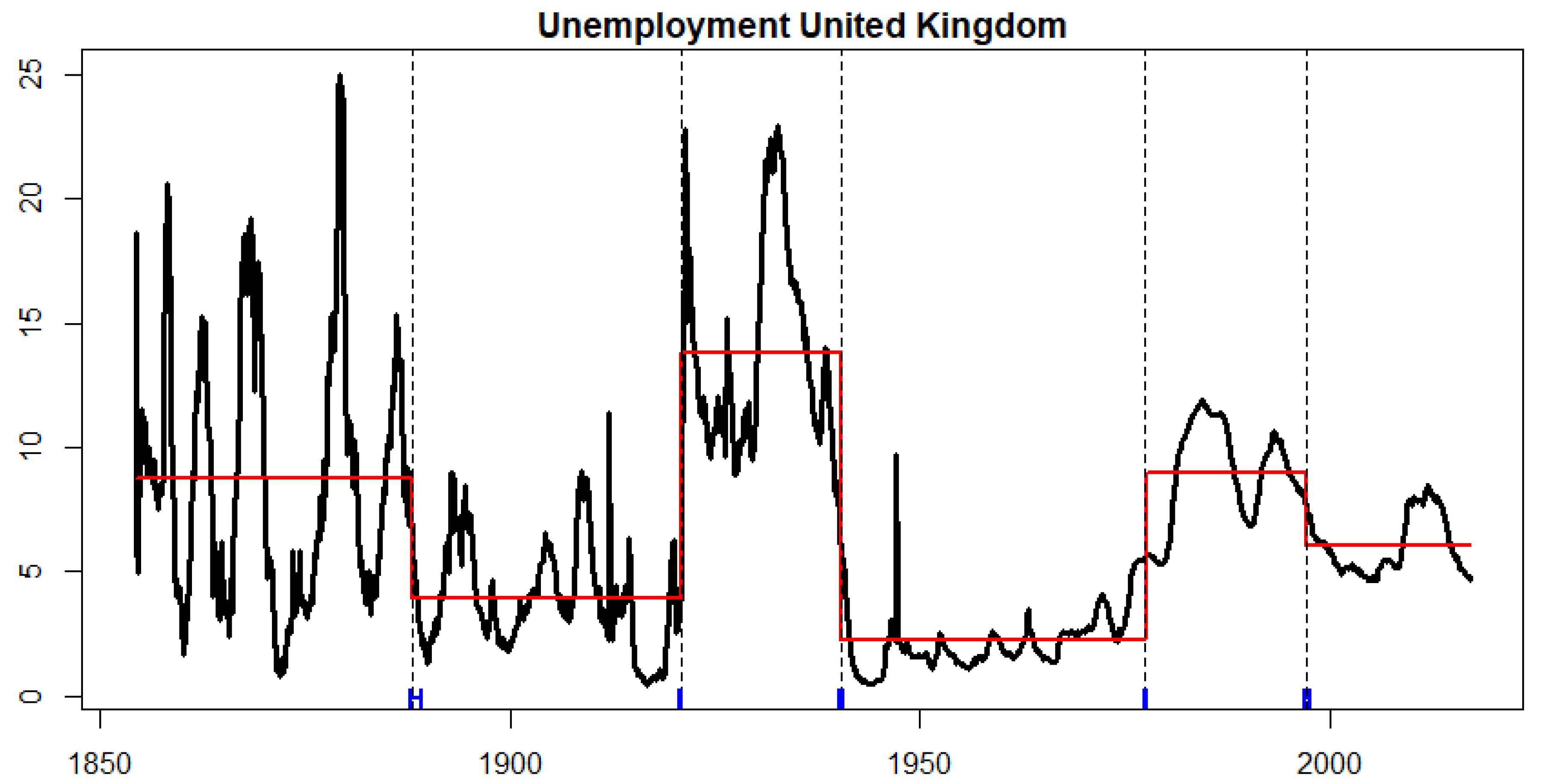
Figure 3 shows the monthly UK unemployment rate from July 1854 to December 2016. Furthermore, the figure shows the structural changes detected by the BP methodology and the mean for each regime. The dates for the structural changes are shown in

Table 5. Dates for structural changes detected by the BP methodology in monthly UK unemployment rates. The confidence intervals are shown below each date.

Estimated date	1888:2	1920:11	1940:5
Confidence interval	[1887:12–1889:04]	[1920:08–1920:12]	[1940:04–1940:07]
Estimated date cont.	1977:6	1996:12
Confidence interval cont.	[1977:04–1977:07]	[1996:10–1997:06]

.

The detected dates relate to major historical events, some of them already discussed for the real GDP per capita series (see Table 1). In particular, we are interested in the long memory properties of the period associated with the Great Pandemic of 1870–1875 and the Russian flu, and the period after the Spanish flu pandemic. The figure shows the higher level of unemployment during the period associated with the Great Pandemic of 1870–1875 and the Russian flu. Moreover, it shows a decrease in unemployment in the following period where no major pandemics are recorded, followed by a rapid increase in unemployment after the Spanish flu pandemic. In this regard, the effects of the Spanish flu pandemic on unemployment are much in line with preliminary estimates for the effects of COVID-19 on unemployment. To better understand the long-run effects of pandemics on unemployment, we first remove the mean for each regime and estimate the persistence of the random component. Results from the long memory estimation are presented in

Table 6. Long memory estimates and change of persistence tests for monthly UK unemployment. The table presents the estimates by both GPH and ELW methods together with their standard errors. Moreover, it presents the critical values for the MR test for the 90%, 95%, and 99% confidence levels, and the associated MR statistic for the test for change in persistence on either direction from the regime in the row above to the current row.

Period	GPH est.	GPH s.e.	ELW est.	ELW s.e.	MR Test
					90%	95%	99%	Stat.
1854:07–1888:02	0.963	0.065	1.137	0.045
1888:03–1920:09	0.825	0.066	0.910	0.046	5.434	6.562	9.553	39.541
1920:10–1940:12	1.018	0.084	1.116	0.056	5.251	6.344	8.966	44.837
1941:01–1976:06	0.518	0.062	0.607	0.044	5.355	6.440	9.084	174.608
1976:07–1996:09	0.682	0.084	0.949	0.056	5.404	6.521	9.200	336.402
1996:10–2016:12	1.109	0.083	1.042	0.056	5.049	6.195	8.901	39.233

.

Table 6 presents the long memory estimates for each regime by the GPH and ELW methods as before. Moreover, it presents the critical values for the MR test for the 90%, 95%, and 99% confidence levels. The last column presents the associated MR statistic for the test for change in persistence on either direction from the regime in the row above to the current row.

Note that unemployment has gone through several changes in the level of persistence across the regimes. Given the shorter span of the unemployment series, we can only analyze the effects of the periods associated with the Great Pandemic of 1870–1875 and Russian flu, and the Spanish flu.

The Great Pandemic of 1870–1875 and the Russian flu are contained in the first period detected. Note that the persistence level estimated in this period is quite high. The confidence intervals for the level of persistence for both estimators contain the $d>1$ value that implies permanent effects on the economy. This contrasts with the persistence level for the subsequent period, where a persistence parameter of $d<1$ is estimated. Furthermore, the MR test for change in persistence rejects the null of no change in persistence. This points to the catastrophic long-lasting effect of the pandemic in unemployment during the Great Pandemic of 1870–1875 and the Russian flu.

Moreover, the long-lasting effects of the Spanish flu pandemic can be seen in the increase in persistence from the 1888:02–1920:09 regime to the 1920:09–1940:12 one. Both GPH and ELW estimates point to an increase in persistence from a value associated with a process that reverts to the mean, $0.5<d<1$, to a value associated with everlasting effects, $d>1$—that is, the period associated with the Spanish flu pandemic seems to have the double effect of increasing the level of unemployment while making it much more persistent. Furthermore, the MR test rejects the null of no change in persistence in either direction at the 99% confidence level. These results may point to the fact that it was much more difficult for survivors to return to work after the pandemic.

In the above discussion, we have associated the increase in unemployment level and persistence to the Spanish flu pandemic. Nonetheless, it could be argued that the First World War is the major historical event behind the results. To shed light on whether major wars may be the main driver behind the increase in unemployment, it is enlightening to see the results from the 1940:12–1976:06 regime, which can be associated with the Second World War. The table shows a decrease in persistence from the regime associated with the Spanish Flu pandemic or First World War to the regime associated with the Second World War. Furthermore, the test for change of persistence strongly rejects the null of no change in persistence. Thus, there seems to be evidence that the period after the Second World War was one of lower, less persistent, unemployment. Contrasting this result with the one associated with the Spanish flu pandemic or First World War suggests that the pandemic plays a significant role in the increased level and persistence of unemployment.

The results on unemployment are of particular interest in light of the current COVID-19 pandemic. As previously noted, governments across the globe decided to implement lockdowns to slow the speed of contagion. The restrictions have substantially impacted several sectors of the economy, like tourism, that no longer needs their staff. The historical evidence found from previous pandemics suggests that, without policies specifically designed to avoid an increase in job losses, we should expect a higher level of unemployment that lasts for an extended period.

As a robustness exercise, first, even though no significant lag at the monthly frequency is found in the autocorrelation function, we deseasonalize the quarterly unemployment rate to explore whether a seasonal component can be interfering in our analysis. Second, we analyze the yearly unemployment rate considering different bandwidths and trimming parameters. The robustness exercises, available upon request, are qualitatively similar to the main exercise presented. Unfortunately, the monthly unemployment series for other countries are not long enough to capture previous pandemics.

4. International Evidence

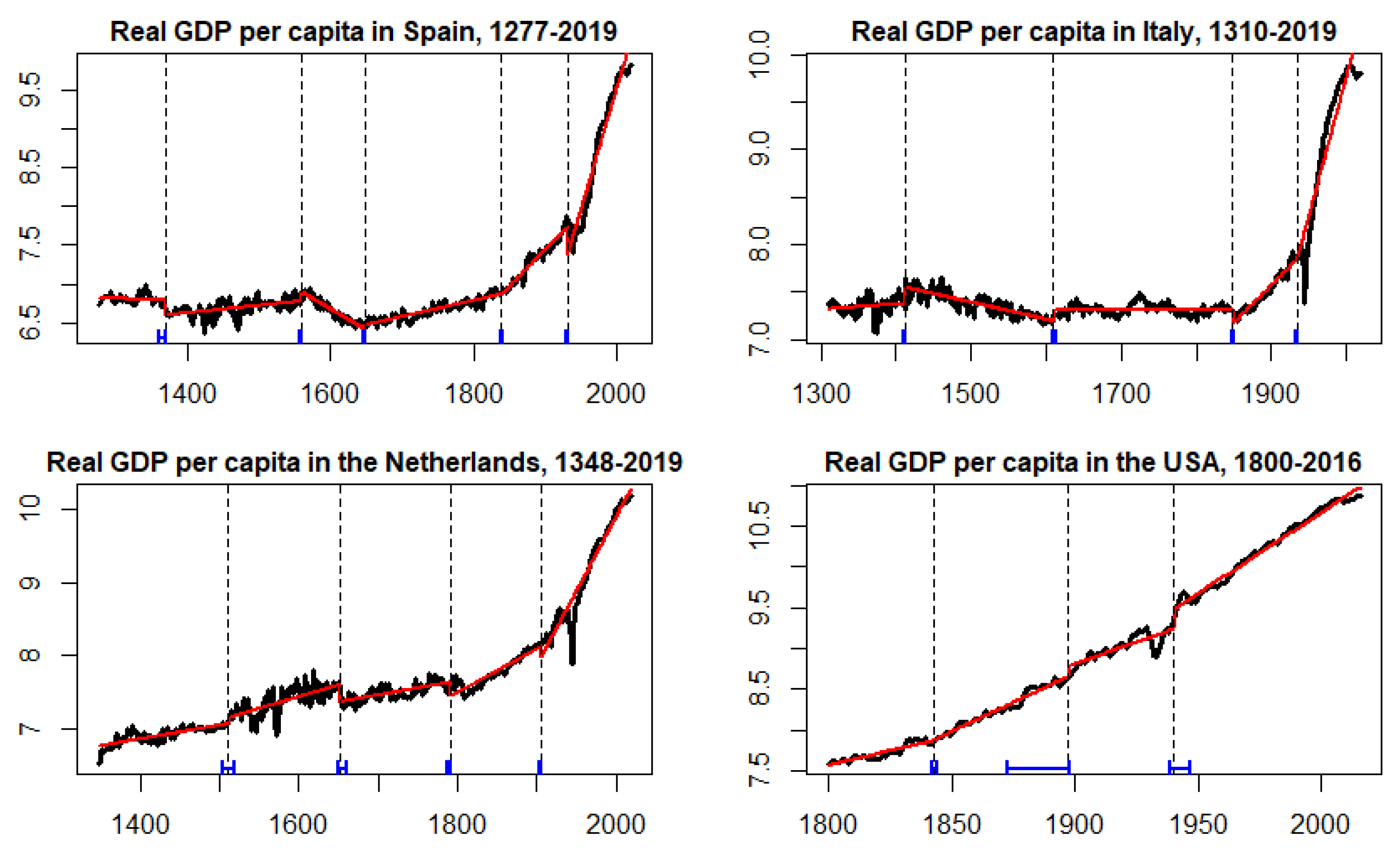
As a robustness exercise, we analyze growth data for other countries for which long economic series are available: Spain, Italy, and the Netherlands. We also use data from the USA given the relevance of the case for our international perspective. The data for Spain comes from Prados de la Escosura et al. (2020), data for Italy, and the Netherlands comes from Conference Board (2020) and Maddison Project of Bolt et al. (2018); while the data for the USA comes from Bolt et al. (2018), published online at OurWorldInData.org.

Figure 4 shows the data and the episodes where each country underwent structural changes as identified by the BP methodology along with their confidence intervals. The results are qualitatively similar to the ones obtained for the UK. In particular, note the changes in trend that occurred in the periods associated with pandemics, signaling their long-lasting effects.

Furthermore,

Table 7. Dates for structural changes detected by the BP methodology in yearly real GDP per capita for Spain, Italy, the Netherlands, and the USA. Column ELW indicates long memory estimates by ELW method, while column MR test shows the MR statistic for the test for change in persistence on either direction from the regime in the row above to the current row. Symbols ${}^{*},{}^{**},$ and ${}^{***}$ denote rejection of the null hypothesis at 10%, 5%, and 1% levels, respectively.

Spain			Italy
Period	ELW	MR Test	Period	ELW	MR Test
1277–1369	1.180		-	-	-
1370–1559	0.455	33.397 ${}^{***}$	1310–1412	0.823
1560–1648	0.337	11.669 ${}^{***}$	1413–1609	0.701	7.423 ${}^{**}$
1649–1838	0.628	10.537 ${}^{***}$	1610–1849	0.573	31.583 ${}^{***}$
1839–1930	0.863	7.611 ${}^{**}$	1850–1934	0.922	3.461
1931–2019	1.377	30.884 ${}^{***}$	1935–2019	1.625	23.212 ${}^{***}$
Netherlands			USA
Period	ELW	MR Test	Period	ELW	MR Test
1348–1511	0.608		-	-	-
1512–1651	0.585	17.134 ${}^{***}$	-	-	-
1652–1791	0.538	6.520 ${}^{**}$	1800–1843	1.090
1792–1905	0.904	9.181 ${}^{**}$	1844–1897	0.920	7.365 ${}^{**}$
-	-	-	1898–1940	1.323	10.477 ${}^{**}$
1906–2019	1.098	38.989 ${}^{***}$	1941–2019	0.999	7.583 ${}^{*}$

shows the long memory estimates for the different periods detected, and tests for change of persistence. We point to three interesting results from Table 7.

First, data from Spain, Italy, and the Netherlands can be used to analyze the effect of the Black Death pandemic. In this regard, note the higher level of persistence for the three countries in periods that contain the pandemic as opposed to the subsequent period. The table shows that the shocks associated with the Black Death pandemic are more persistent than in the subsequent period, pointing to the long-lasting effects of the pandemic.

Second, we note an increase in persistence for the periods that contain the Spanish flu pandemic for all four countries considered—that is, shocks associated with the period around the Spanish flu pandemic appear to be more persistent than in the period before the pandemic, once again pointing to the long-lasting effects of the pandemic on international growth.

Finally, note that the period associated with the Great Plague of London, 1645–1075, is not uncovered for other countries with long economic series besides the UK. As argued in Section 3, this may relate to it being a more localized incident. Using this setting as a counterfactual, these results provide evidence that pandemics seem to be related to the structural changes observed in economic series. Nonetheless, recall that our setting does not allow us to assess causality.

Overall, the results from the data on growth in other countries point in a similar direction to the ones for the UK. Pandemics seem to be related to periods where economic activity suffers structural changes, and their effects appear to be long-lasting.

5. Conclusions

We have analyzed long international series to assess the effect that pandemics have on the economy. We have focused on the United Kingdom given the existence of long economic series for economic growth, measured by real GDP per capita and unemployment. Moreover, we study growth data for other countries to show that the long-lasting effects of pandemics are not restricted to a particular country.

For growth, our results indicate an overall trend upwards in the level of persistence across periods, with significant changes in persistence in the last three centuries. This indicates that, perhaps due to the increased connectivity between countries, contemporaneous outbreaks and pandemics may have longer-lasting effects on growth. Furthermore, qualitatively similar results are found for growth data for Spain, Italy, the Netherlands, and the USA. We highlight the relevance of this finding due to the possible lasting effect that the current epidemic may have on growth for all economies around the world.

In terms of unemployment, we find that the period associated with the Great Pandemic of 1870–1875 and the Russian flu shows a more persistent, higher level of unemployment than in the subsequent period with no major pandemics reported. Moreover, after the Spanish flu pandemic and the First World War, unemployment suffered an increase in level and persistence—that is, unemployment increased, and it became more rooted. This effect is not detected after the Second World War, which points to the relevance of the effect of the shock on unemployment due to the Spanish flu pandemic.

Overall, the findings in this paper strengthen the case for economic policies aimed at softening the shock of the pandemic. Our results show that it is paramount to soften the impact on growth and avoid the loss of jobs to guarantee a V-shaped recovery after COVID-19. The results point to some policy recommendations regarding the economic recovery.

In terms of growth, the high persistence of economic shocks supports the design and implementation of counter-cyclical policies. The high level of persistence in the series suggests that it is more costly to wait after the pandemic to introduce policies to help in the recovery. In this regard, the timing of the intervention is essential. Prompt cash transfers like the one implemented in the USA to sectors of the population more at risk could be implemented to reduce the effect of the pandemic on consumption and GDP.

In terms of unemployment, the increase in level and persistence of unemployment after the pandemic supports the design and implementation of policies that minimize or avoid that companies fire workers during the pandemic. Our results suggest that once the number of unemployed increases, it is a long and arduous process to return to employment levels before the pandemic. This is in line with the notion that the longer people are out of the workforce, the more difficult it is to reintroduce them to the job market. Recently, The Federal Reserve updated its Statement on Longer-Run Goals and Monetary Policy Strategy to indicate that it is willing to accept inflation moderately above 2% for some time and be informed by its assessments of the shortfalls of employment from its maximum level (see The Federal Reserve (2020)). Thus, The Federal Reserve signals the increased priority that it sets on lowering unemployment. In this regard, additional employment policies could be implemented like those deployed in the United Kingdom, the Netherlands, Denmark, and other countries. For instance, the Danish government destined part of its budget to prevent layoffs within private companies facing financial pressures from COVID-19. Under the scheme, the state will cover 75% of the salaries of employees who would otherwise have been fired. Thus, the idea is that once the pandemic recedes, people can go back to work faster. Nonetheless, as was the case for growth, timing is one of the most critical aspects of the implementation.

References

- Abadie, Alberto, Alexis Diamond, and Jens Hainmueller. 2010. Synthetic control methods for comparative case studies: Estimating the effect of california’s tobacco control program. Journal of the American statistical Association 105: 493–505. [Google Scholar] [CrossRef] [Green Version]
- Abadie, Alberto, Alexis Diamond, and Jens Hainmueller. 2015. Comparative politics and the synthetic control method. American Journal of Political Science 59: 495–510. [Google Scholar] [CrossRef]
- Bai, Jushan, and Pierre Perron. 1998. Estimating and testing linear models with multiple structural changes. Econometrica 66: 47–78. [Google Scholar] [CrossRef]
- Bai, Jushan, and Pierre Perron. 2003. Computation and analysis of multiple structural change models. Journal of Applied Econometrics 18: 1–22. [Google Scholar] [CrossRef] [Green Version]
- Beran, Jan, Yuanhua Feng, Sucharita Ghosh, and Rafal Kulik. 2013. Long-Memory Processes: Probabilistic Theories and Statistical Methods. Berlin and Heidelberg: Springer. [Google Scholar] [CrossRef]
- Bolt, Jutta, Robert Inklaar, Herman de Jong, and Jan Luiten van Zanden. 2018. Rebasing Maddison: New income comparisons and the shape of long-run economic development. Maddison Project Database. Available online: https://www.rug.nl/ggdc/historicaldevelopment/maddison/releases/maddison-project-database-2018 (accessed on 1 July 2020).
- Brainerd, Elizabeth, and Mark V Siegler. 2003. The Economic Effects of the 1918 Influenza Epidemic. CEPR Discussion Paper 3791. Available online: https://ssrn.com/abstract=394606 (accessed on 1 July 2020).
- Breitung, Jörg, and Uwe Hassler. 2002. Inference on the cointegration rank in fractionally integrated processes. Journal of Econometrics 110: 167–85. [Google Scholar] [CrossRef] [Green Version]
- Campbell, Bruce M. S., Alexander Klein, Mark Overton, and Bas van Leeuwen. 2015. British Economic Growth, 1270–1870. Cambridge: Cambridge University Press. [Google Scholar]
- Clark, Gregory. 2007. The long march of history: Farm wages, population, and economic growth, England 1209–1869. Economic History Review 60: 97–135. [Google Scholar] [CrossRef] [Green Version]
- Clark, Gregory. 2010. The macroeconomic aggregates for England, 1209–2008. In Research in Economic History. Bingley: Emerald Group Publishing Limited, vol. 27, pp. 51–140. [Google Scholar] [CrossRef] [Green Version]
- Colbourn, Tim. 2020. COVID-19: Extending or relaxing distancing control measures. The Lancet Public Health 5: e236-37. [Google Scholar] [CrossRef] [Green Version]
- Conference Board. 2020. Total Economic Database. Available online: https://www.conference-board.org/data/economydatabase/ (accessed on 1 July 2020).
- Ergemen, Yunus Emre, Niels Haldrup, and Carlos Vladimir Rodríguez-Caballero. 2016. Common long-range dependence in a panel of hourly Nord Pool electricity prices and loads. Energy Economics 60: 79–96. [Google Scholar] [CrossRef]
- Ferguson, Neil, Daniel Laydon, Gemma Nedjati Gilani, Natsuko Imai, Kylie Ainslie, Marc Baguelin, Sangeeta Bhatia, Adhiratha Boonyasiri, ZULMA Cucunuba Perez, Gina Cuomo-Dannenburg, and et al. 2020. Report 9: Impact of Non-Pharmaceutical Interventions (NPIs) to Reduce COVID19 Mortality and Healthcare Demand. Available online: https://www.imperial.ac.uk/media/imperial-college/medicine/mrc-gida/2020-03-16-COVID19-Report-9.pdf (accessed on 1 July 2020).
- Geweke, John, and Susan Porter-Hudak. 1983. The estimation and application of long memory time series models. Journal of Time Series Analysis 4: 221–38. [Google Scholar] [CrossRef]
- Gil-Alana, Luis A, and Peter M Robinson. 1997. Testing of unit root and other nonstationary hypotheses in macroeconomic time series. Journal of Econometrics 80: 241–68. [Google Scholar] [CrossRef] [Green Version]
- Granger, Clive W. J., and R Joyeux. 1980. An introduction to long memory time series models and fractional differencing. Journal of Time Series Analysis 1: 15–29. [Google Scholar] [CrossRef]
- Guerrieri, Veronica, Guido Lorenzoni, Ludwig Straub, and Iván Werning. 2020. Macroeconomic Implications of COVID-19: Can Negative Supply Shocks Cause Demand Shortages? National Bureau of Economic Research WP 26918. Available online: https://ssrn.com/abstract=3569382 (accessed on 1 July 2020).
- Harvey, Andrew, and Stephen Thiele. 2017. Co-Integration and Control: Assessing the Impact of Events Using Time Series Data. Cambrige Working Paper Economics 1731. Cambridge: Cambridge University, Available online: http://www.econ.cam.ac.uk/research-files/repec/cam/pdf/cwpe1731.pdf (accessed on 1 July 2020).
- Hosking, J. R. M. 1981. Fractional differencing. Biometrika 68: 165–76. [Google Scholar] [CrossRef]
- Hurvich, Clifford M., Rohit Deo, and Julia Brodsky. 1998. The mean squared error of Geweke and Porter-Hudak’s estimator of the memory parameter of a long-memory time series. Journal of Time Series Analysis 19: 19–46. [Google Scholar] [CrossRef]
- Jordà, Oscar, Sanjay R. Singh, and Alan M. Taylor. 2020. Longer-Run Economic Consequences of Pandemics. Federal Reserve Bank of San Francisco Working Paper 2020-09. Available online: https://0-doi-org.brum.beds.ac.uk/10.24148/wp2020-09 (accessed on 1 July 2020).
- Karlsson, Martin, Therese Nilsson, and Stefan Pichler. 2014. The impact of the 1918 Spanish flu epidemic on economic performance in Sweden: An investigation into the consequences of an extraordinary mortality shock. Journal of Health Economics 36: 1–19. [Google Scholar] [CrossRef]
- Martins, Luis F., and Paulo M. M. Rodrigues. 2014. Testing for persistence change in fractionally integrated models: An application to world inflation rates. Computational Statistics and Data Analysis 76: 502–22. [Google Scholar] [CrossRef] [Green Version]
- McKibbin, Warwick J., and Roshen Fernando. 2020. The Global Macroeconomic Impacts of COVID-19: Seven Scenarios. Brookings Institution Report. Washington, DC: Brookings Institution, Available online: https://www.brookings.edu/wp-content/uploads/2020/03/20200302_COVID19.pdf (accessed on 1 July 2020).
- Meltzer, Martin I., Nancy J. Cox, and Keiji Fukuda. 1999. The economic impact of pandemic influenza in the United States: Priorities for intervention. Emerging Infectious Diseases 5: 659. [Google Scholar] [CrossRef]
- Nelson, Charles R., and Charles R. Plosser. 1982. Trends and random walks in macroeconmic time series. Some evidence and implications. Journal of Monetary Economics 10: 139–62. [Google Scholar] [CrossRef]
- Osterrieder, Daniela, Daniel Ventosa-Santaulària, and J. Eduardo Vera-Valdés. 2019. The VIX, the variance premium, and expected returns. Journal of Financial Econometrics 17: 517–58. [Google Scholar] [CrossRef] [Green Version]
- Prados de la Escosura, Leandro, Carlos Álvarez-Nogal, and Carlos Santiago-Caballero. 2020. Growth Recurring in Preindustrial Spain: Half a Millennium Perspective. Technical report. England: European Historical Economics Society (EHES). [Google Scholar]
- Prados de la Escosura, Leandro, and Carlos Vladimir Rodríguez-Caballero. 2020. Growth, War, and Pandemics: Europe in the Very Long-Run. EHES Working Paper Series 185. Available online: http://www.ehes.org/EHES_185.pdf (accessed on 1 July 2020).
- Prem, Kiesha, Yang Liu, Timothy W. Russell, Adam J. Kucharski, Rosalind M. Eggo, Nicholas Davies, Stefan Flasche, Samuel Clifford, Carl A. B. Pearson, James D. Munday, and et al. 2020. The effect of control strategies to reduce social mixing on outcomes of the COVID-19 epidemic in Wuhan, China: A modelling study. The Lancet Public Health 5: e61–e270. [Google Scholar] [CrossRef] [Green Version]
- Robinson, Peter M. 1995. Log-periodogram regression of time series with long range dependence. The Annals of Statistics 23: 1048–72. [Google Scholar] [CrossRef]
- Shimotsu, Katsumi, and Peter C. B. Phillips. 2005. Exact local Whittle estimation of fractional integration. The Annals of Statistics 33: 1890–933. [Google Scholar] [CrossRef] [Green Version]
- The Federal Reserve. 2020. Federal Open Market Committee announces approval of updates to its Statement on Longer-Run Goals and Monetary Policy Strategy [Press Release]. Available online: https://www.federalreserve.gov/newsevents/pressreleases/monetary20200827a.htm (accessed on 27 August 2020).
- Thomas, R., and N. Dimsdale. 2017. A milllenium of UK data. Bank of England Datasets. Available online: https://0-www-bankofengland-co-uk.brum.beds.ac.uk/statistics/research-datasets (accessed on 1 July 2020).
- Varneskov, Rasmus T., and Pierre Perron. 2018. Combining long memory and level shifts in modelling and forecasting the volatility of asset returns. Quantitative Finance 18: 371–93. [Google Scholar] [CrossRef]
- Vera-Valdés, J. Eduardo. 2020. On long memory origins and forecast horizons. Journal of Forecasting 39: 811–26. [Google Scholar] [CrossRef] [Green Version]
Figure 1.
Real GDP per capita for the UK, 1270–2019 (in logs). Breaks are represented by the vertical black dashed lines, while their confidence intervals at 95% are displayed by blue small intervals in the bottom of the figure. BP methodology with a trimming parameter of is executed.
Figure 2.
Real GDP per capita for the UK, 1645–1800 (in logs). The break is represented by the vertical black dashed line. The counterfactual values are computed by forecasting the linear trend with long memory disturbances estimated in the period associated with the Great Plague of London.
Figure 3.
UK monthly unemployment rates. Breaks are represented by the vertical black dashed lines, while their confidence intervals at 95% are displayed by blue small intervals in the bottom of the figure. BP methodology with a trimming parameter of is executed.
Figure 4.
Real GDP per capita for Spain, Italy, the Netherlands, and the USA (in logs). Breaks are represented by the vertical black dashed lines, while their confidence intervals at 95% are displayed by blue small intervals in the bottom of the figure.