Direct and Indirect Effects under Sample Selection and Outcome Attrition

Abstract

This paper extends the evaluation of direct and indirect treatment effects, i.e., mediation analysis, to the case that outcomes are only partially observed due to sample selection or outcome attrition. We assume sequential conditional independence of the treatment and the mediator, i.e., the variable through which the indirect effect operates. We also impose missing at random or instrumental variable assumptions on the outcome attrition process. Under these conditions, we derive identification results for the effects of interest that are based on inverse probability weighting by specific treatment, mediator, and/or selection propensity scores. We also provide a simulation study and an empirical application to the U.S. Project STAR data in which we assess the direct impact and indirect effect (via absenteeism) of smaller kindergarten classes on math test scores. The estimators considered are available in the ‘causalweight’ package for the statistical software ‘R’.

1. Introduction

Mediation analysis, i.e., the evaluation of direct and indirect causal effects, is widespread in social sciences, following the seminal papers (Baron and Kenny 1986; Judd and Kenny 1981; Robins and Greenland 1992). The aim is to disentangle the total causal effect of a treatment on an outcome of interest into an indirect component operating through one or several intermediate variables, i.e., mediators, as well as a direct component. As example, consider the effect of educational interventions on health, where part of the effect might be mediated by health behaviors, see (Brunello et al. 2016), or personality traits, see (Conti et al. 2016). While earlier studies on mediation typically rely on tight linear models, the more recent literature considers more flexible and possibly nonlinear specifications. A large number of contributions assumes sequential conditional independence, implying that the assignment of the treatment and the mediator is conditionally exogenous given observed covariates and given the treatment and the covariates, respectively. For examples, see (Pearl 2001; Petersen et al. 2006; Robins 2003; Albert and Nelson 2011; Flores and Flores-Lagunes 2009; Hong 2010; Huber 2014a; Imai et al. 2010; Tchetgen and Shpitser 2012; VanderWeele 2009; Vansteelandt et al. 2012; Zheng and van der Laan 2012), among many others.

In this paper, we extend mediation analysis to account for the complication of outcome nonresponse and sample selection, implying that outcomes are only observed for a subset of the initial population of interest. Such problems frequently occur in empirical applications like wage gap decompositions, where wages are only observed for those who work. In a range of studies evaluating total (rather than direct and indirect) effects, sample selection is assumed to be missing at random (MAR), i.e., conditionally exogenous given observed variables, see for instance (Abowd et al. 2001; Little and Rubin 1987; Rubin 1976; Robins et al. 1994, 1995; Carroll et al. 1995; Fitzgerald et al. 1998; Shah et al. 1997; Wooldridge 2002, 2007). In contrast, nonignorable nonresponse models permit sample selection to be related to unobservables. Unless strong parametric assumptions are imposed (see for instance (Heckman 1976, 1979; Hausman and Wise 1979; Little 1995)), identification requires an instrumental variable (IV) for sample selection (e.g., Das et al. 2003; Newey 2007; Huber 2012, 2014b).

In this paper, we combine the evaluation of average natural direct and indirect effects based on sequential conditional independence with specific MAR or IV assumptions about sample selection. We identify the parameters of interest in the total as well as the selected population (whose outcomes are actually observed) by inverse probability weighting1 (IPW) based on propensity scores for treatment and selection. Under MAR, effects in the total population are obtained through reweighing by the inverse of the selection propensity given observed characteristics. If selection is related to unobservables, we make use of a control function that can be regarded as a nonparametric version of the inverse Mill’s ratio in Heckman-type selection models. Under specific conditions, reweighing observations by the inverse of the selection propensity given observed characteristics and the control function identifies the effects in the selected or the total population. To convey the intuition of our identification results, we provide a brief simulation study in which the propensity scores are estimated by probit models.

As an empirical illustration, we evaluate the average natural direct and indirect effects of Project STAR, an educational experiment in Tennessee, which randomly assigned children to small classes in kindergarten and primary school. The positive impact of STAR classes on academic achievement has been demonstrated for example in (Krueger 1999), but less is known about the underlying causal mechanisms. We consider absenteeism in kindergarten as potential mediator of the effect. The outcome of interest is the score in a standardized math test in the first grade of primary school, which is unobserved for a non-negligible share of children due to attrition. We apply one of our proposed IPW-based estimators to account for outcome attrition and compare the results to several alternative mediation estimators that make no corrections for sample selection. The results suggest that absenteeism is not an important driver of the total effect.2

The remainder of this paper is organized as follows. Section 2 discusses the parameters of interest, the assumptions, and the nonparametric identification results based on inverse probability weighting. Section 3 outlines estimation based on the sample analogs of the identification results. Section 4 presents a simulation study. Section 5 provides an application to Project STAR data. Section 6 concludes the paper.

2. Identification

2.1. Parameters of Interest

We would like to disentangle the average treatment effect (ATE) of a binary treatment variable D on an outcome variable Y into a direct effect and an indirect effect operating through the mediator M, which has bounded support and may be a scalar or a vector and discrete and/or continuous. To define the effects of interest, we use the potential outcome framework, see (Rubin 1974), which has been applied in the context of mediation analysis by (Rubin 2004; Ten Have et al. 2007; Albert 2008), among others. $M\left(d\right)andY(d,M\left(d^{\prime }\right))$ denote the potential mediator state as a function of the treatment and potential outcome as a function of the treatment and the potential mediator, respectively, under treatments $d,d^{\prime }$∈$\{0,1\}$. Only one potential outcome and mediator state, respectively, are observed for each unit, because the realized mediator and outcome values are $M=D·M\left(1\right)+(1-D)·M\left(0\right)$ and $Y=D·Y(1,M(1\left)\right)+(1-D)·Y(0,M(0\left)\right)$.

The ATE is given by $\Delta =E\left[Y\right(1,M\left(1\right))-Y(0,M\left(0\right)\left)\right]$. To disentangle the latter, note that the (average) natural direct effect (using the denomination of (Pearl 2001))3 is identified by exogenously varying the treatment but keeping the mediator fixed at its potential value for $D=d$:

$$\begin{array}{ccc}\hfill \theta \left(d\right)& =& E\left[Y\right(1,M\left(d\right))-Y(0,M\left(d\right)\left)\right],d\in \{0,1\},\hfill \end{array}$$

(1)

Equivalently, by exogenously shifting the mediator to its potential values under treatment and non-treatment but keeping the treatment fixed at $D=d$, the (average) natural indirect effect4 is obtained:

$$\begin{array}{ccc}\hfill \delta \left(d\right)& =& E\left[Y\right(d,M\left(1\right))-Y(d,M\left(0\right)\left)\right],d\in \{0,1\}.\hfill \end{array}$$

(2)

The ATE is the sum of the direct and indirect effects defined upon opposite treatment states:

$$\begin{array}{ccc}\hfill \Delta & =& E\left[Y\right(1,M\left(1\right))-Y(0,M\left(0\right)\left)\right]\hfill \\ & =& E\left[Y\right(1,M\left(1\right))-Y(0,M\left(1\right)\left)\right]+E\left[Y\right(0,M\left(1\right))-Y(0,M\left(0\right)\left)\right]=\theta \left(1\right)+\delta \left(0\right)\hfill \\ & =& E\left[Y\right(1,M\left(0\right))-Y(0,M\left(0\right)\left)\right]+E\left[Y\right(1,M\left(1\right))-Y(1,M\left(0\right)\left)\right]=\theta \left(0\right)+\delta \left(1\right).\hfill \end{array}$$

(3)

This follows from adding and subtracting $E\left[Y\right(0,M\left(1\right)\left)\right]$ or $E\left[Y\right(1,M\left(0\right)\left)\right]$, respectively. The notation $\theta \left(1\right),\theta \left(0\right)$ and $\delta \left(1\right),\delta \left(0\right)$ points to possible effect heterogeneity w.r.t. the potential treatment state, implying the presence of interaction effects between the treatment and the mediator. However, the effects cannot be identified without further assumptions, as either $Y(1,M(1\left)\right)$ or $Y(0,M(0\left)\right)$ is observed for any unit, whereas $Y(1,M(0\left)\right)$ and $Y(0,M(1\left)\right)$ are never observed.

In contrast to natural effects, which are functions of the potential mediators, the so-called controlled direct effect is obtained by setting the mediator to a predetermined value m, rather than $M\left(d\right)$:

$$\begin{array}{ccc}\hfill \gamma \left(m\right)& =& E\left[Y\right(1,m)-Y(0,m\left)\right],m\mathrm{in\; the\; support\; of}M.\hfill \end{array}$$

(4)

Whether $\theta \left(d\right)$ or $\gamma \left(m\right)$ is of primary interest depends on the research question at hand. The controlled direct effect may provide policy guidance whenever mediators can be externally prescribed, as for instance in a sequence of active labor market programs assigned by a caseworker, where D and M denote assignment of the first and second program, respectively. This allows analyzing the direct effect of the first program under alternative combinations of program prescriptions. In contrast, the natural direct effect assesses the effectiveness of the first program given the status quo decision to participate in the second program in the light of participation or non-participation in the first program. We refer to (Pearl 2001) for further discussion of what he calls the descriptive and prescriptive natures of natural and controlled effects.

Our identification results will make use of a vector of observed covariates, denoted by X, that may confound the causal relations between D and M, D and Y, and M and Y. A further complication in our evaluation framework is that Y is assumed to be observed for a subpopulation, i.e., conditional on $S=1$, where S is a binary variable indicating whether Y is observed/selected, or not. We therefore also define the direct and indirect effects among the selected population:

$$\begin{array}{ccc}\hfill {\theta }_{S=1}\left(d\right)& =& E[Y(1,M\left(d\right))-Y(0,M\left(d\right))|S=1],{\delta }_{S=1}\left(d\right)=E[Y(d,M\left(1\right))-Y(d,M\left(0\right))|S=1],\hfill \\ \hfill {\gamma }_{S=1}\left(m\right)& =& E\left[Y\right(1,m)-Y(0,m\left)\right|S=1].\hfill \end{array}$$

Empirical examples with partially observed outcomes include wage regressions, with S being an employment indicator, see for instance (Gronau 1974), or the evaluation of the effects of policy interventions in education on test scores, with S being participation in the test, see (Angrist et al. 2006). Throughout our discussion, S is allowed to be a function of D, M, and X, i.e., $S=S(D,M,X)$. However, S must neither be affected by nor affect Y.5 S is therefore not a mediator, as selection per se does not causally influence the outcome. An example for such a set up in terms of nonparametric structural models is given by

$$\begin{array}{c}\hfill Y=\varphi (D,M,X,U),S=\psi (D,M,X,V),\end{array}$$

(5)

where $U,V$ are unobserved characteristics and $\varphi ,\psi$ are general functions.6

2.2. Assumptions and Identification Results under MAR

This section presents identifying assumptions that formalize the sequential conditional independence of D and M as imposed by (Imai et al. 2010) and many others as well as an MAR restriction on Y that implies that S is related to observables.7

Assumption 1

(conditional independence of the treatment). (a) $Y(d,m)\perp D|X=x$, (b) $M\left(d^{\prime }\right)\perp D|X=x$ for all $d,d^{\prime }\in \{0,1\}$ and $m,x$ in the support of $M,X$.

By Assumption 1, there are no unobservables jointly affecting the treatment, on the one hand, and the mediator and/or the outcome, on the other hand, conditional on X. In observational studies, the plausibility of this assumption crucially hinges on the richness of the data, while in experiments, it is satisfied if the treatment is randomized within strata defined by X or randomized independently of X.8

Assumption 2

(conditional independence of the mediator). $Y(d,m)\perp M|D=d^{\prime },X=x$ for all $d,d^{\prime }\in \{0,1\}$ and $m,x$ in the support of $M,X$.

By Assumption 2, there are no unobservables jointly affecting the mediator and the outcome conditional on D and X. Assumption 2 only appears realistic if detailed information on possible confounders of the mediator-outcome relation is available in the data (even in experiments with random treatment assignment) and if post-treatment confounders of M and Y can be plausibly ruled out when controlling for D and X.9

Assumption 3

(conditional independence of selection). $Y\perp S|D=d,M=m,X=x$ for all $d\in \{0,1\}$ and $m,x$ in the support of $M,X$.

By Assumption 3, there are no unobservables jointly affecting selection and the outcome conditional on $D,M,X$, such that outcomes are missing at random (MAR) in the denomination of (Rubin 1976). Put differently, selection is assumed to be selective w.r.t. observed characteristics only.

Assumption 4

(common support). (a) $Pr(D=d|M=m,X=x)>0$ and (b) $Pr(S=1|D=d,$$M=m,X=x)>0$ for all $d\in \{0,1\}$ and $m,x$ in the support of $M,X$.

Assumption 4(a) is a common support restriction requiring that the conditional probability to receive a specific treatment given $M,X$, henceforth referred to as propensity score, is larger than zero in either treatment state. It follows that $Pr(D=d|X=x)>0$ must hold, too. By Bayes’ theorem, Assumption 4(a) implies that $Pr(M=m|D=d,X=x)>0$, or in the case of M being continuous, that the conditional density of M given $D,X$ is larger than zero. Conditional on X, M must not be deterministic in D, as otherwise identification fails due to the lack of comparable units in terms of the mediator across treatment states. Assumption 4(b) requires that for any combination of $D,M,X$, the probability to be observed is larger than zero. Otherwise, the outcome is not observed for some specific combinations of these variables implying yet another common support issue.

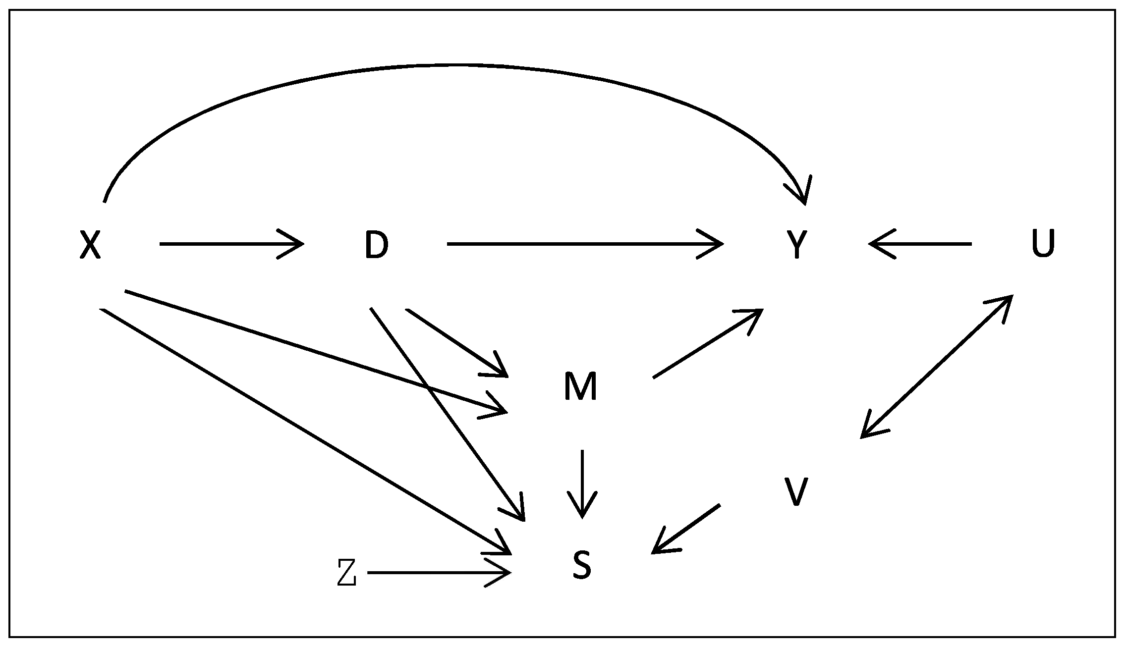
Figure 1 illustrates the causal framework underlying our assumptions by means of a causal graph, see for instance (Pearl 1995), in which each arrow represents a potential causal effect. Further (unobserved) variables that only affect one of the variables explicitly displayed in the system are kept implicit. For instance, there may be unobservable variables U that affect the outcome, but do not influence D, M, or S; otherwise, there would be confounding. Under Assumptions 1 to 4, potential outcomes as well as direct and indirect effects in the total population are identified based on weighting by the inverse of the treatment and selection propensity scores.

Theorem 1.

(i) 

Under Assumptions 1–4, for d∈$\{0,1\}$,

$$\begin{array}{ccc}\hfill E\left[Y\right(d,M(1-d)\left)\right]& =& E\left[\frac{Y·I\{D=d\}·S}{Pr(D=d|M,X)·Pr(S=1|D,M,X)}·\frac{Pr(D=1-d|M,X)}{Pr(D=1-d|X)}\right],\hfill \\ \hfill E\left[Y\right(d,M\left(d\right)\left)\right]& =& E\left[\frac{Y·I\{D=d\}·S}{Pr(D=d|X)·Pr(S=1|D,M,X)}\right].\hfill \end{array}$$

(6)

(ii) 

Under Assumptions 1(a), 2–4, and M following a discrete distribution,

$$\begin{array}{c}\hfill E\left[Y(d,m)\right]=E\left[\frac{Y·I\{D=d\}·I\{M=m\}·S}{Pr(D=d|X)·Pr(M=m|D,X)·Pr(S=1|D,M,X)}\right].\end{array}$$

(7)

Proof. 

See Appendix A. □

Using the results of Theorem 1, it can be easily shown that the direct and indirect effects are identified by

$$\begin{array}{ccc}\hfill \theta \left(d\right)& =& E\left[\left(\frac{Y·D}{Pr(D=1|M,X)}-\frac{Y·(1-D)}{1-Pr(D=1|M,X)}\right)·\frac{Pr(D=d|M,X)·S}{Pr(D=d|X)·Pr(S=1|D,M,X)}\right],\hfill \\ \hfill \delta \left(d\right)& =& E\left[\frac{Y·I\{D=d\}·S}{Pr(D=d|M,X)·Pr(S=1|D,M,X)}·\left(\frac{Pr(D=1|M,X)}{Pr(D=1|X)}-\frac{1-Pr(D=1|M,X)}{1-Pr(D=1|X)}\right)\right],\hfill \\ \hfill \gamma \left(m\right)& =& E\left[\left(\frac{Y·D}{Pr(D=1|X)}-\frac{Y·(1-D)}{1-Pr(D=1|X)}\right)·\frac{I\{M=m\}·S}{Pr(M=m|D,X)·Pr(S=1|D,M,X)}\right].\hfill \end{array}$$

These expressions are related to the IPW-based identification in (Huber 2014a) for the case with no missing outcomes with the difference that here, multiplication by $S/Pr(S=1|D,M,X)$ is included to account for sample selection. Furthermore, our results fit into the general framework of (Wooldridge 2002), who considers the IPW-based M-estimation of missing data models. Finally, for the identification of $\gamma \left(m\right)$, Assumption 1 can be relaxed to Assumption 1(a) because (in contrast to $\theta \left(d\right),\delta \left(d\right)$) the distribution of the potential mediator $M\left(d\right)$ need not be identified.

2.3. Assumptions and Identification Results under Selection Related to Unobservables

In the following discussion, we consider the case that selection is related to both observables and unobservables that are associated with the outcome. Assumptions 3 and 4 are therefore replaced. Rather, we assume that an instrumental variable for S is available to tackle sample selection.

Assumption 5

(instrument for selection). (a) There exists an instrument Z that may be a function of $D,M$, i.e., $Z=Z(D,M)$, is conditionally correlated with S, i.e., $E[Z·S|D,M,X]\ne 0$, and satisfies (i) $Y(d,m,z)=Y(d,m)$ and (ii) $\{Y(d,m),M\left(d^{\prime }\right)\}\perp Z(d^{″},m^{\prime })|X=x$ for all $d,d^{\prime },d^{″}\in \{0,1\}$, and $m,m^{\prime },x$ in the support of $M,X$. (b) $S=I\{V\le \Pi (D,M,X,Z\left)\right\}$, where Π is a general function and V is a scalar (index of) unobservable(s) with a strictly monotonic cumulative distribution function conditional on X, (c) $V\perp (D,M,Z)|X$.

Assumption 5 no longer imposes the independence of Y and S given observed characteristics. As the unobservable V in the selection equation is allowed to be associated with unobservables affecting the outcome, Assumptions 1 and 2 generally do not hold conditional on $S=1$ due to the endogeneity of the post-treatment variable S. In fact, $S=1$ implies that $\Pi (D,M,X,Z)>V$ such that conditional on X, the distribution of V generally differs across values of $D,M$. This entails a violation of the sequential conditional independence assumptions on $D,M$ given $S=1$ if potential outcome distributions differ across values of V. We, therefore, require an instrumental variable denoted by Z, which is allowed to be affected by D and M, but must not affect Y or be associated with unobservables affecting M or Y, as invoked in (5a).10 We apply a control function approach based on this instrument,11 which requires further assumptions.

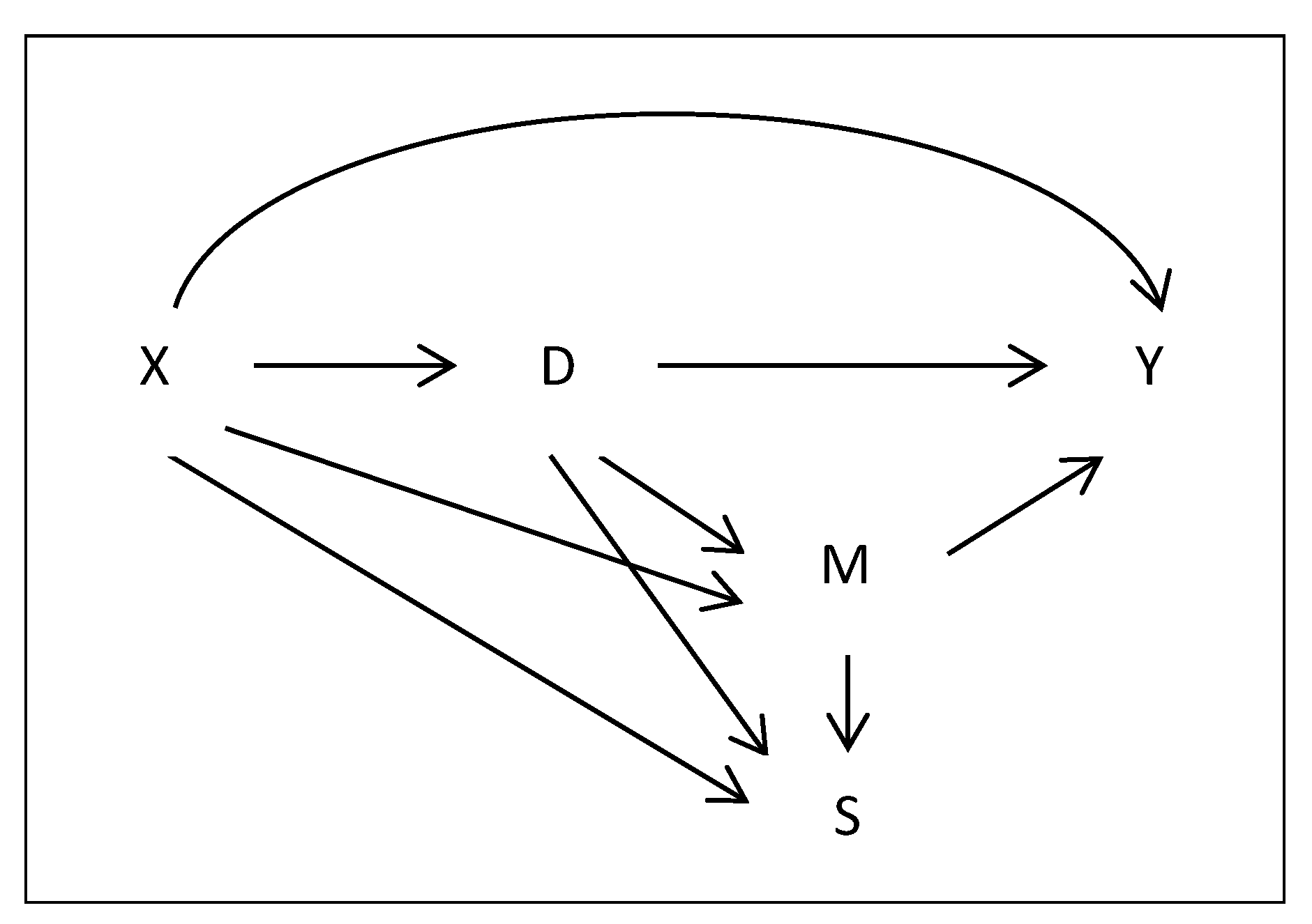
By the threshold crossing model postulated in 5(b), $Pr(S=1|D,M,X,Z)=Pr(V\le \Pi (D,M,X,Z))=F_V(\Pi (D,M,X,Z))$, where $F_V\left(v\right)$ denotes the cumulative distribution function of V evaluated at v. We will henceforth use the notation $p\left(W\right)=Pr(S=1|D,M,X,Z)$ with $W=D,M,X,Z$ for the sake of brevity. Again by Assumption 5(b), the selection probability $p\left(W\right)$ increases strictly monotonically in $\Pi$ conditional on X, such that there is a one-to-one correspondence between the distribution function $F_V$ and specific values v given X. By Assumption 5(c), V is independent of $(D,M,Z)$ given X, implying that the distribution function of V given X is (nonparametrically) identified. Figure 2 illustrates the causal framework underlying Assumptions 1, 2, and 5 by means of a causal graph.

By comparing individuals with the same $p\left(W\right)$, we control for $F_V$ and thus for the confounding associations of V with (i) D and $\{Y(d,m),M\left(d^{\prime }\right)\}$ and (ii) M and $Y(d,m)$ that occur conditional on $S=1$. In other words, $p\left(W\right)$ serves as control function where the exogenous variation comes from Z. Controlling for the distribution of V based on the instrument is thus a feasible alternative to the (infeasible) approach of directly controlling for levels of V. More concisely, it follows from our assumptions for any bounded function g that

$$\begin{array}{ccc}& & E\left[g\left(Y\right(d,m\left)\right)|D,M,X,p(W),S=1\right]=E\left[g\left(Y(d,m)\right)|D,M,X,F_V,S=1\right]\hfill \\ & & =E\left[g\left(Y(d,m)\right)|D,X,F_V,S=1\right]=E\left[g\left(Y(d,m)\right)|X,F_V,S=1\right].\hfill \end{array}$$

The first equality follows from $p\left(W\right)=F_V$ under Assumption 5, the second from the fact that when controlling for $F_V$, conditioning on $S=1$ does not result in an association between $Y(d,m)$ and M given $D,X$ such that $Y(d,m)\perp M|D,X,p(W),S=1$ holds by Assumptions 2 and 5. This is due to the fact that conditional on $p\left(W\right)$ (or $F_V$), there are no unobservables that are jointly related with S and Y. Therefore, conditioning on $S=1$ when also controlling for $p\left(W\right)$ does not introduce a statistical association between M and unobservables affecting Y (a phenomenon known as collider or sample selection bias). The third equality follows from the fact that when controlling for $F_V$, conditioning on $S=1$ does not result in an association between $Y(d,m)$ and D given X such that $Y(d,m)\perp D|X,p(W),S=1$ holds by Assumptions 1 and 5.12 Similarly,

$$\begin{array}{c}\hfill E\left[g\left(M\right(d\left)\right)|D,X,p(W),S=1\right]=E\left[g\left(M\left(d\right)\right)|D,X,F_V,S=1\right]=E\left[g\left(M\left(d\right)\right)|X,F_V,S=1\right]\end{array}$$

follows from the fact that when controlling for $F_V$, conditioning on $S=1$ does not result in an association between $M\left(d\right)$ and D given X such that $M\left(d\right)\perp D|X,p(W),S=1$ holds by Assumptions 1 and 5. These results will be useful in the proofs of Theorems 2 and 3, see Appendix A.2.

Furthermore, identification requires the following common support assumption, which is similar to Assumption 4(a), but in contrast to the latter also includes $p\left(W\right)$ as a conditioning variable.

Assumption 6

(common support). $Pr(D=d|M=m,X=x,p\left(W\right)=p\left(w\right),S=1)>0$ for all $d\in \{0,1\}$ and $m,x,z$ in the support of $M,X,Z$.

By Bayes’ theorem, Assumption 6 implies that the conditional density of $p\left(W\right)=p\left(w\right)$ given $D,M,X,S=1$ is larger than zero. This means that in fully nonparametric contexts, the instrument Z must in general be continuous and strong enough to importantly shift the selection probability $p\left(W\right)$ conditional on $D,M,X$ in the selected population. Assumptions 1, 2, 5, and 6 are sufficient for the identification of mean potential outcomes as well as direct and indirect effects in the selected population.

Theorem 2.

(i) 

Under Assumptions 1, 2, 5, and 6 for d∈$\{0,1\}$,

$$\begin{array}{ccc}\hfill E\left[Y\right(d,M(1-d)\left)\right|S=1]& =& E\left[\frac{Y·I\{D=d\}}{Pr(D=d|M,X,p\left(W\right))}·\frac{Pr(D=1-d|M,X,p\left(W\right))}{Pr(D=1-d|X,p\left(W\right))}|S=1\right],\hfill \\ \hfill E\left[Y\right(d,M\left(d\right)\left)\right|S=1]& =& E\left[\frac{Y·I\{D=d\}}{Pr(D=d|X,p\left(W\right))}|S=1\right].\hfill \end{array}$$

(8)

(ii) 

Under Assumptions 1(a), 2, 5, and 6, and M following a discrete distribution,

$$\begin{array}{ccc}\hfill E\left[Y\right(d,m\left)\right|S=1]& =& E\left[\frac{Y·I\{D=d\}·I\{M=m\}}{Pr(D=d|X,p\left(W\right))·Pr(M=m|D,X,p(W\left)\right)}|S=1\right].\hfill \end{array}$$

(9)

Proof. 

See Appendix A. □

Therefore, the direct and indirect effects are identified by

$$\begin{array}{ccc}\hfill {\theta }_{S=1}\left(d\right)& =& E\left[\left(\frac{Y·D}{Pr(D=1|M,X,p\left(W\right))}-\frac{Y·(1-D)}{1-Pr(D=1|M,X,p\left(W\right))}\right)·\frac{Pr(D=d|M,X,p\left(W\right))}{Pr(D=d|X,p\left(W\right))}|S=1\right],\hfill \\ \hfill {\delta }_{S=1}\left(d\right)& =& E\left[\frac{Y·I\{D=d\}}{Pr(D=d|M,X,p\left(W\right))}·\left(\frac{Pr(D=1|M,X,p\left(W\right))}{Pr(D=1|X,p\left(W\right))}-\frac{1-Pr(D=1|M,X,p\left(W\right))}{1-Pr(D=1|X,p\left(W\right))}\right)|S=1\right],\hfill \\ \hfill {\gamma }_{S=1}\left(m\right)& =& E\left[\left(\frac{Y·D}{Pr(D=1|X,p\left(W\right))}-\frac{Y·(1-D)}{1-Pr(D=1|X,p\left(W\right))}\right)·\frac{I\{M=m\}}{Pr(M=m|D,X,p\left(W\right))}|S=1\right].\hfill \end{array}$$

In nonparametric models that allow for general forms of effect heterogeneity related to unobservables, direct and indirect effects can generally only be identified among the selected population. The reason is that effects among selected observations cannot be extrapolated to the non-selected population if the effects of D and M interact with unobservables affecting the outcome, henceforth denoted by U, as the latter are in general distributed differently across $S=1,0$ even conditional on observed variables. To see this, note that conditional on $p\left(W\right)=Pr(V\le \Pi (D,M,X,Z\left)\right)$, the distribution of V differs across the selected (satisfying $V\le \Pi (D,M,X,Z)$) and the non-selected (satisfying $V>\Pi (D,M,X,Z)$), such that the distribution of U differs, too, if V and U are associated. While control function $p\left(W\right)$ is required for the unconfoundedness of the treatment and the mediator in the selected subpopulation, it does not permit extrapolating effects to the population with unobserved outcomes, see also (Huber and Melly 2015) for further discussion.

The identification of effects in the total population therefore requires additional assumptions. In Assumption 7 below, we impose homogeneity in the direct and indirect effects across selected and non-selected populations conditional on $X,V$. A sufficient condition for effect homogeneity is the separability of observed and unobserved components in the outcome variable, i.e., $Y=\eta (D,M,X)+\nu \left(U\right)$, where $\eta ,\nu$ are general functions. Furthermore, common support as postulated in Assumption 6 needs to be strengthened to hold in the entire population. In addition, the selection probability $p\left(w\right)$ must be larger than zero for any w in the support of W; otherwise, outcomes are not observed for some values of $D,M,X$. Assumption 8 formalizes these common support restrictions.

Assumption 7

(conditional effect homogeneity). $E\left[Y\right(1,m)-Y(0,m\left)\right|X=x,V=v,S=1]=E[Y(1,m)-Y(0,m)|X=x,V=v]$ and $E\left[Y\right(d,M\left(1\right))-Y(d,M\left(0\right)\left)\right|X=x,V=v,S=1]=E[Y(d,M(1\left)\right)-Y(d,M(0\left)\right)|X=x,V=v]$, for all $d\in \{0,1\}$ and $m,x,v$ in the support of $M,X,V$.

Assumption 8

(common support). (a) $Pr(D=d|M=m,X=x,p\left(W\right)=p\left(w\right))>0$ and (b) $p\left(w\right)>0$ for all $d\in \{0,1\}$ and $m,x,z$ in the support of $M,X,Z$.

While the mean potential outcomes in the total population remain unknown even under Assumptions 7 and 8, the effects of interest are nevertheless identified by the separability of U.

Theorem 3.

(i) Under Assumptions 1, 2, 5, 6, 7, and 8 for d∈$\{0,1\}$,

$$\begin{array}{ccc}\hfill \theta \left(d\right)& =& E\left[\left(\frac{Y·D}{Pr(D=1|M,X,p\left(W\right))}-\frac{Y·(1-D)}{1-Pr(D=1|M,X,p\left(W\right))}\right)·\frac{Pr(D=d|M,X,p\left(W\right))·S}{Pr(D=d|X,p\left(W\right))·p(W)}\right]\hfill \\ \hfill \delta \left(d\right)& =& E\left[\frac{Y·I\{D=d\}·S}{Pr(D=d|M,X,p\left(W\right))·p(W)}·\left(\frac{Pr(D=1|M,X,p\left(W\right))}{Pr(D=1|X,p\left(W\right))}-\frac{1-Pr(D=1|M,X,p\left(W\right))}{1-Pr(D=1|X,p\left(W\right))}\right)\right].\hfill \end{array}$$

(10)

(ii) Under Assumptions 1(a), 2, 5–8, and M following a discrete distribution,

$$\begin{array}{ccc}\hfill \gamma \left(m\right)& =& E\left[\left(\frac{Y·D}{Pr(D=1|X,p\left(W\right))}-\frac{Y·(1-D)}{1-Pr(D=1|X,p\left(W\right))}\right)·\frac{I\{M=m\}·S}{Pr(M=m|D,X,p\left(W\right))·p(W)}\right].\hfill \end{array}$$

(11)

Proof. 

See Appendix A. □

We conclude our discussion on identification by informally sketching an instrumental variable approach when the treatment D is not conditionally independent as postulated in Assumption 1. Consider for instance an experiment in which the access to the treatment is randomized, but actual treatment participation may endogenously deviate from the granted access based on unobserved characteristics. If Assumption 1 holds for the access variable, it may serve as instrument for treatment participation under the additional assumptions that it shifts the treatment weakly monotonically and has no direct effect on the outcome other than through the treatment. Imbens and Angrist (1994); Angrist et al. (1996) show that in the absence of sample selection, these assumptions permit identifying a local ATE (LATE) in the subpopulation of compliers, i.e., among those whose treatment status reacts to the instrument. This requires scaling the so-called intention-to-treat or reduced form effect of the instrument on the outcome by the first stage effect of the instrument on the treatment.

Adding further complications to the identification problem like sample selection and/or mediation requires appropriately modifying the expression of the intention-to-treat effect before scaling it by the first stage. See for instance (Frölich and Huber 2014), who evaluate the LATE when assuming that sample selection is not associated with unobserved characteristics conditional on observables alone or conditional on observables and the compliance type (i.e., under latent ignorability, see (Frangakis and Rubin 1999)). Alternatively, Fricke et al. (2020) discuss identification when sample selection is associated with unobservables based on distinct instruments for the treatment and selection. In the absence of sample selection, Frölich and Huber (2017) consider disentangling the LATE into direct and indirect effects when an instrument for the mediator is available (in addition to that for the treatment). A combination of such approaches permits jointly tackling sample selection and mediator endogeneity in instrumental variable frameworks and is left for future research.

2.4. Extensions to Further Populations, Parameters, and Variable Distributions

This section briefly discusses how the identification results can be extended to further populations of interest, policy-relevant parameters, and richer distributions of the treatment and/or the mediator. First and in analogy to the concept of weighted treatment effects in (Hirano et al. 2003), direct and indirect effects can be identified for particular target populations defined upon covariates X by reweighing observations according to the distribution of X in the target population. To this end, we define $\omega \left(X\right)$ to be a well-behaved weighting function depending on X. Including $\frac{\omega \left(X\right)}{E\left[\omega \right(X\left)\right]}$ in the expectation operators presented in the theorems above yields the parameters of interest for the target population. As an important example, consider $\omega \left(X\right)=Pr(D=1|X)$. For some well-behaved function $f(Y,D,M,S,X,Z)$ of the observed data,

$$\begin{array}{cc}\hfill & E\left[\frac{\omega \left(X\right)}{E\left[\omega \right(X\left)\right]}·f(Y,D,M,S,X,Z)\right]=E\left[\frac{Pr(D=1|X)}{Pr(D=1)}·f(Y,D,M,S,X,Z)\right]\\ & =E\left[\frac{Pr(D=1|X)}{Pr(D=1)}·f(Y,D,M,S,X,Z)\right]=E\left[f(Y,D,M,S,X,Z)|D=1\right],\end{array}$$

(12)

i.e., the expected value of that function among the treated is identified. Likewise, defining $\omega \left(X\right)=1-Pr(D=1|X)$ gives the expected value among the non-treated. Any of the expressions in the expectation operators of the theorems may serve as $f(Y,D,M,S,X,Z)$ in (12).13

Second, the identification results may be extended to well-behaved functions of Y, rather than Y itself. For instance, replacing Y by $I\{Y\le a\}$, the indicator function that Y is not larger than some value a, everywhere in the theorems permits identifying distributional features or effects. The inversion of potential outcome distribution functions allows identifying quantile treatment effects.

Third, our framework can be adapted to allow for multiple or multivalued (rather than binary) treatments. If D is multivalued discrete, the derived expressions may be applied under minor adjustments. For instance, for any $d\ne d^{\prime }$ in the discrete support of D, the expression for potential outcomes in Theorem 1 becomes

$$\begin{array}{c}\hfill E\left[Y(d,M\left(d^{\prime }\right))\right]=E\left[\frac{Y·I\{D=d\}·S}{Pr(D=d|M,X)·Pr(S=1|D,M,X)}·\frac{Pr(D=d^{\prime }|M,X)}{Pr(D=d^{\prime }|X)}\right]\end{array}$$

under appropriate common support conditions. If D is continuous, any indicator functions for treatment values, which are only appropriate in the presence of mass points, need to be replaced by kernel functions, while treatment propensity scores need to be substituted by conditional density functions. In analogy to (Hsu et al. 2018), who consider mediation analysis with continuous treatments in the absence of sample selection, the expression for potential outcomes in Theorem 1 becomes

$$\begin{array}{ccc}\hfill E\left[Y(d,M\left(d^{\prime }\right))\right]& =& \underset{h\to 0}{lim}E\left[\frac{Y·\omega (D;d,h)·S}{E\left[\omega \right(D;d,h\left)\right|M,X]·Pr(S=1|D,M,X)}\right.\hfill \\ & \times & \left.\frac{E\left[\omega (D;d^{\prime },h)\right|M,X]}{E\left[\omega (D;d^{\prime },h)\right|X]}\right].\hfill \end{array}$$

The weighting function $\omega (D;d)=K\left((D-d)/h\right)/h$, with K being a symmetric second order kernel function assigning more weight to observations closer to d and h being a bandwidth operator. For h going to zero, i.e., ${lim}_{h\to 0}$, $E\left[\omega (D;d^{\prime },h)\right|X]$ and $E\left[\omega (D;d^{\prime },h)\right|M,X]$ correspond to the conditional densities of D given X and given $M,X$, respectively, also known as generalized propensity scores. We refer to (Hsu et al. 2018) for more discussion on direct and indirect effects of continuous treatments and how estimation may proceed based on generalized propensity scores. We also note that in the context of controlled direct effects, such kernel methods not only allow for a continuous treatment, but (contrarily to our theorems) also for a continuous mediator.

3. Estimation

The parameters of interest can be estimated using the normalized versions of the sample analogs of the IPW-based identification results in Section 2. This implies that the weights of the observations used for the computation of mean potential outcomes add up to unity, as advocated in (Busso et al. 2009; Imbens 2004). For instance, the normalized sample analogs of the results in Theorem 1, part (i) are given by

$$\begin{array}{ccc}{\widehat{\mu }}_{1,M\left(0\right)}\hfill & =\hfill & \frac{1}{n}\sum _{i=1}^n\frac{Y_i·D_i·S_i}{\widehat{p}(M_i,X_i)·\widehat{\pi }(D_i,M_i,X_i)}\frac{1-\widehat{p}(M_i,X_i)}{1-\widehat{p}\left(X_i\right)}/\frac{1}{n}\sum _{i=1}^n\frac{D_i·S_i}{\widehat{p}(M_i,X_i)·\widehat{\pi }(D_i,M_i,X_i)}\frac{1-\widehat{p}(M_i,X_i)}{1-\widehat{p}\left(X_i\right)},\hfill \\ {\widehat{\mu }}_{0,M\left(1\right)}\hfill & =\hfill & \frac{1}{n}\sum _{i=1}^n\frac{Y_i·(1-D_i)·S_i}{(1-\widehat{p}(M_i,X_i))·\widehat{\pi }(D_i,M_i,X_i)}\frac{\widehat{p}(M_i,X_i)}{\widehat{p}\left(X_i\right)}/\frac{1}{n}\sum _{i=1}^n\frac{(1-D_i)·S_i}{(1-\widehat{p}(M_i,X_i))·\widehat{\pi }(D_i,M_i,X_i)}\frac{\widehat{p}(M_i,X_i)}{\widehat{p}\left(X_i\right)},\hfill \\ {\widehat{\mu }}_{1,M\left(1\right)}\hfill & =\hfill & \frac{1}{n}\sum _{i=1}^n\frac{Y_i·D_i·S_i}{\widehat{p}\left(X_i\right)·\widehat{\pi }(D_i,M_i,X_i)}/\frac{1}{n}\sum _{i=1}^n\frac{D_i·S_i}{\widehat{p}\left(X_i\right)·\widehat{\pi }(D_i,M_i,X_i)},\hfill \\ {\widehat{\mu }}_{0,M\left(0\right)}\hfill & =\hfill & \frac{1}{n}\sum _{i=1}^n\frac{Y_i·(1-D_i)·S_i}{(1-\widehat{p}\left(X_i\right))·\widehat{\pi }(D_i,M_i,X_i)}/\frac{1}{n}\sum _{i=1}^n\frac{(1-D_i)·S_i}{(1-\widehat{p}\left(X_i\right))·\widehat{\pi }(D_i,M_i,X_i)}.\hfill \end{array}$$

i indexes observations in an i.i.d. sample of size n and ${\widehat{\mu }}_{d,M\left(d^{\prime }\right)}$ is an estimate of ${\mu }_{d,M\left(d^{\prime }\right)}=E\left[Y(d,M\left(d^{\prime }\right))\right]$ with $d,d^{\prime }$∈$\{1,0\}$. $\widehat{p}(M_i,X_i)$, $\widehat{p}\left(X_i\right)$ are estimates of the treatment propensity scores $Pr(D=1|M_i,X_i)$, $Pr(D=1|X_i)$, respectively, while $\widehat{\pi }(D_i,M_i,X_i)$ is an estimate of the selection propensity score $Pr(S=1|D,M,X)$. Direct and indirect effect estimates are obtained by $\widehat{\theta }\left(d\right)={\widehat{\mu }}_{1,M\left(d\right)}-{\widehat{\mu }}_{0,M\left(d\right)}$ and $\widehat{\delta }\left(d\right)={\widehat{\mu }}_{d,M\left(1\right)}-{\widehat{\mu }}_{d,M\left(0\right)}$.

When propensity scores are estimated parametrically, e.g., based on probit models as in the simulations and application below, then ${\widehat{\mu }}_{d,M\left(d^{\prime }\right)},\widehat{\theta }\left(d\right),\widehat{\delta }\left(d\right)$ satisfy the sequential GMM framework discussed in (Newey 1984), with propensity score estimation representing the first step and parameter estimation the second step. This approach is $\sqrt{n}$-consistent and asymptotically normal under standard regularity conditions. When the propensity scores are estimated nonparametrically, $\sqrt{n}$-consistency and asymptotic normality can be obtained if the first step estimators satisfy particular regularity conditions. See (Hsu et al. 2017), who consider series logit estimation of the propensity scores, however, for the case without sample selection. Furthermore, the bootstrap is consistent for inference as the proposed IPW estimators are smooth and asymptotically normal.

The suggested IPW estimators are computationally inexpensive and straightforwardly permit considering multiple mediators. On the negative side, IPW-based estimation is sensitive to (estimation errors in) propensity scores that are very close to one or zero, see the simulation results in (Busso et al. 2009; Frölich 2004) as well as the theoretical discussion in (Khan and Tamer 2010). This sensitivity can lead to an explosion in the variance and numerical instability in finite samples. Furthermore, as the propensity score directly enters the expression for estimating the potential outcomes or treatment effects, IPW may be less robust to propensity score misspecification than for instance propensity score matching, which merely uses the score to match observations across treatment states, see (Waernbaum 2012). This suggests the use of sufficiently flexible propensity score specifications, while the sensitivity issue can be tackled by trimming too extreme propensity scores, see (Crump et al. 2009), at the cost of somewhat reducing external validity.

4. Simulation Study

This section provides a brief simulation study, in which we investigate the finite sample properties of estimation of natural direct and indirect effects based on the sample analogs of Theorems 1 to 3. To this end, the following data generating process is considered:

$$\begin{array}{ccc}\hfill Y& =\hfill & 0.5D+M+0.5DM+X-\alpha DU+U,Y\mathrm{is}\mathrm{observed}\mathrm{if}S=1,\hfill \\ \hfill S& =\hfill & I\{0.5D-0.5M+0.25X+Z+V>0\},\hfill \\ \hfill M& =\hfill & 0.5D+0.5X+W,D=I\{0.5X+Q>0\},Z=0.25X-0.25M+R,\hfill \\ \hfill X,U,V,W,Q,R& \sim \hfill & \mathcal{N}(0,1),\mathrm{independently}\mathrm{of}\mathrm{each}\mathrm{other}.\hfill \end{array}$$

The outcome Y is a linear function of the observed variables $D,M,X$ and an unobserved term U, and is only observed if the selection indicator S—which depends on $D,M,X$, an instrument Z, and an unobservable V—is equal to one. $\alpha$ gauges the interaction of D and U in the outcome equation. For $\alpha \ne 0$, the treatment effect is heterogeneous in U such that Assumption 7 is violated. W and R denote the unobservables in the linearly modeled mediator M and instrument Z, respectively. Any unobservable as well as the observed covariate X are standard normally distributed independent of each other. In this framework, the assumptions underlying Theorem 1 are satisfied.

We run 5000 Monte Carlo simulations with sample sizes $n=1000,4000$ and consider estimation of the natural direct and indirect effects in the total population ($\theta \left(d\right)$, $\delta \left(d\right)$) based on three different estimators: (i) normalized IPW as suggested in (Huber 2014a) among the selected (‘IPW w. $S=1$’) that controls for X but ignores selection bias, (ii) normalized IPW based on Theorem 1 assuming MAR (IPW MAR), and (iii) normalized IPW based on Theorem 3 (IPW IV). We estimate the treatment and selection propensity scores by probit and apply a trimming rule that discards observations with $\widehat{p}(M,X)$ smaller than 0.05 or larger than 0.95 or with $\widehat{\pi }(D,M,X)$ smaller than 0.05 to prevent exploding weights due to small denominators. Trimming hardly affects IPW estimator (i), but reduces the variance of estimation based on Theorems 1 and 3 in several cases.

Table 1. Simulations under selection on observables, total population.

	$\widehat{\mathit{\theta }}\left(1\right)$			$\widehat{\mathit{\theta }}\left(0\right)$			$\widehat{\mathit{\delta }}\left(1\right)$			$\widehat{\mathit{\delta }}\left(0\right)$
	bias	std	rmse	bias	std	rmse	bias	std	rmse	bias	std	rmse
	$\alpha =0.25$, $n=1000$
IPW w. $S=1$	−0.16	0.14	0.21	−0.17	0.16	0.23	−0.01	0.15	0.15	−0.02	0.11	0.12
IPW MAR	0.03	0.28	0.28	0.01	0.20	0.20	−0.03	0.13	0.14	−0.05	0.14	0.15
IPW IV	−0.01	0.30	0.30	−0.02	0.31	0.31	−0.02	0.18	0.18	−0.03	0.15	0.15
	$\alpha =0.25$, $n=4000$
IPW w. $S=1$	−0.16	0.07	0.18	−0.17	0.08	0.19	0.00	0.08	0.08	−0.01	0.06	0.06
IPW MAR	0.01	0.15	0.15	0.01	0.10	0.10	−0.02	0.07	0.07	−0.03	0.08	0.09
IPW IV	−0.01	0.15	0.15	−0.02	0.16	0.16	−0.01	0.09	0.09	−0.02	0.08	0.08

Note: std and rmse report the standard deviation and root mean squared error, respectively.

reports the simulations results under $\alpha =0.25$,14 namely the bias, standard deviation (std), and the root mean squared error (RMSE) of the various estimators for the natural direct and indirect effects in the total population. Ignoring selection (IPW w. $S=1$) yields biased estimates of the direct effects under either sample size, while biases are generally small for estimation based on Theorem 1. Interestingly, the latter result also holds for estimation related to Theorem 3, where the selection process accounts for the same observed factors as under the correct MAR assumption, plus the control function. Even though including the control function is not required for consistency, it does not jeopardize identification either, even if Assumption 7 requiring $\alpha =0$ is not satisfied,15 as reflected in the low biases. However, accounting for this unnecessary variable entails an increase of the standard deviation in some cases. In general, the estimators based on Theorems 1 and 3 are (due to the estimation of the sample selection propensity score) less precise than IPW without selection correction in the selected sample. The proposed methods become relatively more competitive in terms of the RMSE as the sample size increases and gains in bias reduction become relatively more important compared to losses in precision.

As a modification to our initial setup, we introduce a correlation between U and V, which implies that the assumptions underlying Theorem 1 no longer hold, while those of Theorem 2 are satisfied and those of Theorem 3 are satisfied when $\alpha =0$:

$$\begin{array}{ccc}\left(\begin{array}{c}U\\ V\end{array}\right)\hfill & \sim \hfill & \mathcal{N}(\mu ,\Sigma ),\mathrm{where}\mu =\left(\begin{array}{c}0\\ 0\end{array}\right)\mathrm{and}\Sigma =\left(\begin{array}{cc}1& 0.8\\ 0.8& 1\end{array}\right)\hfill \end{array}$$

Table 2. Simulations with selection on unobservables, total population.

	$\widehat{\mathit{\theta }}\left(1\right)$			$\widehat{\mathit{\theta }}\left(0\right)$			$\widehat{\mathit{\delta }}\left(1\right)$			$\widehat{\mathit{\delta }}\left(0\right)$
	bias	std	rmse	bias	std	rmse	bias	std	rmse	bias	std	rmse
	$\alpha =0$, $n=1000$
IPW w. $S=1$	−0.28	0.13	0.31	−0.27	0.16	0.32	0.07	0.16	0.18	0.07	0.12	0.14
IPW MAR (Theorem 1)	−0.09	0.30	0.31	−0.11	0.21	0.24	0.06	0.14	0.15	0.04	0.15	0.16
IPW IV (Theorem 3)	0.02	0.32	0.32	−0.01	0.31	0.31	−0.02	0.18	0.18	−0.05	0.16	0.16
	$\alpha =0$, $n=4000$
IPW w. $S=1$	−0.28	0.07	0.29	−0.28	0.08	0.29	0.08	0.08	0.12	0.09	0.06	0.11
IPW MAR (Theorem 1)	−0.11	0.16	0.20	−0.11	0.10	0.15	0.06	0.07	0.09	0.06	0.09	0.11
IPW IV (Theorem 3)	0.01	0.17	0.17	−0.01	0.16	0.16	−0.02	0.09	0.09	−0.04	0.08	0.09
	$\alpha =0.25$, $n=1000$
IPW w. $S=1$	−0.37	0.13	0.39	−0.35	0.15	0.38	0.05	0.16	0.16	0.07	0.12	0.14
IPW MAR (Theorem 1)	−0.20	0.30	0.36	−0.20	0.21	0.28	0.03	0.14	0.14	0.04	0.15	0.16
IPW IV (Theorem 3)	−0.14	0.32	0.34	−0.16	0.31	0.35	−0.02	0.18	0.18	−0.05	0.16	0.16
	$\alpha =0.25$, $n=4000$
IPW w. $S=1$	−0.38	0.07	0.38	−0.36	0.08	0.36	0.06	0.08	0.10	0.09	0.06	0.11
IPW MAR (Theorem 1)	−0.22	0.16	0.27	−0.20	0.10	0.22	0.04	0.07	0.08	0.06	0.09	0.11
IPW IV (Theorem 3)	−0.14	0.16	0.22	−0.16	0.16	0.23	−0.01	0.09	0.09	−0.04	0.08	0.09

Note: std and rmse report the standard deviation and root mean squared error, respectively.

reports the results for the estimation of natural effects in the total population under $\alpha =0$ and $0.25$ using the same methods as before. Non-negligible biases occur not only when ignoring sample selection (IPW w. $S=1$), but also when selection is assumed to be related to observables only (IPW MAR). When $\alpha =0$, estimation based on Theorem 3 (IPW IV) is close to being unbiased and dominates the other methods in terms of RMSE under the larger sample size ($n=4000$). When $\alpha =0.25$, however, also the latter approach is biased due to the violation of Assumption 7. Therefore,

Table 3. Simulations with selection on unobservables, selected population ($S=1$).

	${\widehat{\mathit{\theta }}}_{\mathit{S}=1}\left(1\right)$			${\widehat{\mathit{\theta }}}_{\mathit{S}=1}\left(0\right)$			${\widehat{\mathit{\delta }}}_{\mathit{S}=1}\left(1\right)$			${\widehat{\mathit{\delta }}}_{\mathit{S}=1}\left(0\right)$
	bias	std	rmse	bias	std	rmse	bias	std	rmse	bias	std	rmse
	$\alpha =0.25$, $n=1000$
IPW w. $S=1$	−0.11	0.13	0.17	−0.09	0.15	0.17	0.05	0.16	0.16	0.07	0.12	0.14
IPW IV w. $S=1$ (Theorem 2)	0.00	0.21	0.21	−0.03	0.23	0.23	0.02	0.17	0.17	−0.01	0.12	0.12
	$\alpha =0.25$, $n=4000$
IPW w. $S=1$	−0.12	0.07	0.14	−0.10	0.08	0.12	0.06	0.08	0.10	0.09	0.06	0.11
IPW IV w. $S=1$ (Theorem 2)	0.01	0.10	0.10	−0.02	0.11	0.12	0.03	0.08	0.08	−0.00	0.06	0.06

Note: std and rmse report the standard deviation and root mean squared error, respectively.

considers the estimation of natural effects among the selected population only (${\theta }_{S=1}\left(d\right)$, ${\delta }_{S=1}\left(1\right)$) in the presence of the D-U-interaction effect. We investigate the performance of estimation based on Theorem 2 (IPW IV w. $S=1$), as well as of IPW among the selected ignoring selection. While the latter approach is biased, the former is close to being unbiased, but less precise. The relative performance of the IV method in terms of the RMSE improves as the sample size (and thus precision) increases.16

However, it needs to be pointed out that the usefulness of the instrument-based estimator might be limited in many empirical applications. In our simulations, IPW IV has the highest variance among the methods considered, which may outweigh the gains in terms of a smaller bias and thus entail a higher RMSE in particular in moderate samples. Furthermore, the high variance issue becomes considerably more severe if the instrument is weak and has (in contrast to our simulation design) only a limited effect on selection, at least when controlling for multiple covariates. In such realistic scenarios, the biased IPW MAR method has most likely a smaller RMSE than the unbiased, but unstable IPW IV estimator. Nevertheless, the instrumental variable approach appears useful in research designs with randomly assigned instruments (that are sufficiently strong), e.g., financial incentives for responding in follow-up surveys such as vouchers, cash payments, or cash lotteries. See for instance (Castiglioni et al. 2008; Hsu et al. 2017; Pforr et al. 2015).

5. Empirical Application

This section illustrates the evaluation of direct and indirect treatment effects in the presence of sample selection using data from Project Student–Teacher Achievement Ratio (STAR), an educational experiment conducted from 1985 to 1989 in Tennessee, USA. In the experiment, a cohort of students entering kindergarten and their teachers were randomly assigned within their school to one of three class types: small (13–17 students), regular (22–26 students), or regular with an additional teacher’s aid. Students were supposed to remain in the assigned class type through third grade, returning to regular classes afterwards. The goal of Project STAR was investigating the impact of class size on academic achievement measured by standardized and curriculum-based tests in mathematics, reading, and basic study skills. Numerous studies found positive effects of reduced class size on academic performance both short- (Finn and Achilles 1990; Folger and Breda 1989; Krueger 1999), mid- (Finn et al. 1989; Krueger and Whitmore 2001; Nye et al. 2001), and even on later-life outcomes (Chetty et al. 2011). While benefits of small class size are well documented, the causal mechanisms underlying the effect are less well-understood. Finn and Achilles (1990) argue that the impact is likely driven by classroom processes related to higher teacher morale and satisfaction translated to students, increased teacher–student interactions and time for individual attention, and student involvement in learning activities.

We investigate whether the effect of reduced class size on academic performance is mediated by the number of days absent from school. There might be several explanations for why class size affects days of absence. A smaller concentration of children in a classroom may be related to reduced transmission of infectious diseases and hence absenteeism.17 Increased student involvement and closer teacher–student relationships in smaller classes may represent further channels making children and their parents more engaged and less likely to miss classes. As for the link between school absence and academic performance, a number of studies demonstrated a negative association between the two, see for instance (Gershenson et al. 2017; Gottfried 2009; Morrissey et al. 2014).

We compare results using the IPW MAR estimator (IPW MAR in Table 5) based on Theorem 1 (relying on Assumptions 1 through 4) in Section 2 to three previously considered mediation estimators that ignore sample selection:18 (i) a linear mediation estimator allowing for treatment–mediator interactions but neither accounting for observed pre-treatment confounders, nor selection, which is numerically equivalent to the decomposition of (Blinder 1973; Oaxaca 1973) (Lin w. $S=1$, no X);19 (ii) a semiparametric IPW-based analog of the linear mediation estimator not accounting for confounding also considered in (Huber 2015) (IPW w. $S=1$, no X); and (iii) the IPW estimator suggested in (Huber 2014a) that incorporates observed pre-treatment covariates X but ignores sample selection when estimating the effect for the total population (IPW w. $S=1$). We apply the same trimming rule as in the simulations presented in Section 4, which discards observations with treatment propensity scores $\widehat{p}(M,X)$ smaller than 0.05 or larger than 0.95 or with $\widehat{\pi }(D,M,X)$ smaller than 0.05. However, no observations are dropped for any IPW method as such extreme propensity scores do not occur in our sample.

The treatment (D) is a binary indicator which is one if a child entering kindergarten was enrolled in a small class and zero otherwise.20 The outcome (Y) is the first grade score in the Stanford Achievement Test (SAT) in mathematics. For IPW MAR estimation, a selection indicator S for missing outcomes is generated and all observations in our evaluation sample are preserved, such that effects are estimated for the entire population. In the case of the remaining three estimators, the evaluation is based on the data with non-missing Y, such that estimation relies on the selected sample only. The mediator (M) is the number of days a child was absent during the kindergarten year. Observed covariates (X) consist of a child’s race, gender, year of birth, and free lunch status as a proxy for socio-economic status. They are controlled for in the IPW w. $S=1$ and IPW MAR estimators. Even if these variables are initially balanced due to the random assignment of D, they might confound M and Y, implying that they are imbalanced when conditioning on the mediator for estimating direct and indirect effects.21

We restrict the initial sample of 11,601 children to 6325 observations who were part of Project STAR in kindergarten such that their treatment status was observed.22 About 30% of participants in the kindergarten year were randomized into small classes.

Table 4. Mean covariate values by treatment status.

Variable	Total	$\mathit{d}=0$	$\mathit{d}=1$	Difference	p-Value
Student’s gender: male	0.51	0.51	0.51	0.00	0.96
	[0.50]	[0.50]	[0.50]	(0.01)
Student’s race: white	0.67	0.67	0.68	0.01	0.42
	[0.47]	[0.47]	[0.47]	(0.02)
Free lunch	0.48	0.49	0.47	−0.02	0.25
	[0.50]	[0.50]	[0.50]	(0.02)
Born 1978	0.01	0.01	0.00	−0.01	0.00
	[0.08]	[0.09]	[0.05]	(0.00)
Born 1979	0.23	0.22	0.25	0.03	0.04
	[0.42]	[0.42]	[0.43]	(0.01)
Born 1980	0.76	0.77	0.74	−0.02	0.09
	[0.43]	[0.42]	[0.44]	(0.01)
Born 1981	0.00	0.00	0.00	0.00	0.87
	[0.03]	[0.03]	[0.03]	(0.00)
Kindergarten days absent	10.51	10.72	10.01	−0.71	0.02
	[9.76]	[9.95]	[9.29]	(0.31)
Math SAT grade 1	534.54	531.52	541.25	9.73	0.00
	[43.83]	[42.92]	[45.10]	(2.14)

Note: Standard deviations are in squared brackets. Cluster-robust standard errors are in parentheses.

presents summary statistics for the variables included in our empirical illustration for individuals without any missing values in the covariates. It shows a positive and statistically significant association between reduced class size and the average score in the standardized math test. Furthermore, children in small classes are, on average, about 0.7 days less absent. This difference is significant at the 5% level, but arguably small in terms of absolute magnitude. There are no statistically significant differences in students’ gender, race,23, and free lunch status across treatment states due to treatment randomization. The sample is not perfectly balanced in terms of students’ year of birth: children born in 1978 and 1980 were less likely to be in small classes (differences are statistically significant at the 1 and 10% levels, respectively), while those born in 1979 were more likely to be in small classes (significant at the 5% level). There is substantial attrition: math SAT scores in the first grade are observed for only 70% of program participants in the kindergarten year. The number of missing values in other key variables is much smaller. In the estimations, observations with missing values in M or X are dropped, which concerns all in all 83 cases, or about 1% of the sample.

Table 5. Effects of small class size in kindergarten on the math Stanford Achievement Test (SAT) in grade 1.

	Total Effect			$\widehat{\mathit{\theta }}\left(1\right)$			$\widehat{\mathit{\theta }}\left(0\right)$			$\widehat{\mathit{\delta }}\left(1\right)$			$\widehat{\mathit{\delta }}\left(0\right)$
	est.	s.e.	$\mathit{p}$-Value	est.	s.e.	$\mathit{p}$-Value	est.	s.e.	$\mathit{p}$-Value	est.	s.e.	$\mathit{p}$-Value	est.	s.e.	$\mathit{p}$-Value
IPW MAR	8.74	2.37	0.00	8.52	2.36	0.00	7.75	2.70	0.00	0.99	0.79	0.21	0.23	0.13	0.09
Lin w. $S=1$, no X	9.73	2.16	0.00	9.46	2.17	0.00	9.55	2.15	0.00	0.27	0.18	0.12	0.18	0.13	0.16
IPW w. $S=1$, no X	9.73	2.16	0.00	9.55	2.15	0.00	9.43	2.18	0.00	0.30	0.21	0.16	0.18	0.13	0.15
IPW w. $S=1$	9.20	2.14	0.00	9.01	2.14	0.00	8.77	2.19	0.00	0.43	0.32	0.18	0.19	0.14	0.18

Note: Cluster-robust standard errors (s.e.) and p-values (p-value) for the point estimates (est.) are obtained by bootstrapping the latter 1999 times.

provides point estimates (est.), cluster-robust standard errors (s.e.) based on blockbootstrapping the effects 1999 times, and p-values for the total treatment effect, as well as natural direct and indirect effects under treatment and non-treatment ($\widehat{\theta }\left(1\right)$, $\widehat{\theta }\left(0\right)$, $\widehat{\delta }\left(1\right)$, $\widehat{\delta }\left(0\right)$) for the four estimators. The total average effect of small class assignment is very similar across all methods and highly statistically significant, amounting to an increase of almost 10 points. Furthermore, we find that, if anything, the contribution of the indirect effects due to reduced days of absence is rather small, ranging 0.18 to 0.99 points across different methods and treatment states. This is not surprising in the light of the quite modest differences in absenteeism across treatment groups, see Table 4. The IPW MAR estimator yields the largest indirect effects (amounting to 3–11% of the total effect), and the indirect effect on the non-treated group is statistically significant at the 10% level. It is thus the direct effects, which are highly statistically significant for any method, that mostly drive the total effect. IPW MAR yields direct effect estimates of 8.52 points under treatment and 7.75 points under non-treatment, which is slightly smaller than those of the other estimators exploiting the subsample with non-missing outcomes only (ranging from 9.01 to 9.55 points under treatment and from 8.77 to 9.55 points under non-treatment). We therefore conclude that causal mechanisms not observed in the data (possibly including teacher motivation and individual teacher–student interaction) and entering the direct effect are much more important than absenteeism for explaining the effect of small kindergarten classes on math performance.

6. Conclusions

In this paper, we proposed an approach for disentangling a total causal effect into a direct component and a indirect effect operating through a mediator in the presence of outcome attrition or sample selection. To this end, we combined sequential conditional independence assumptions about the assignment of the treatment and the mediator with either selection on observables/missing at random or instrumental variable assumptions on the outcome attrition process. We demonstrated the identification of the parameters of interest based on inverse probability weighting by specific treatment, mediator, and/or selection propensity scores and outlined estimation based on the sample analogs of these results. We also provided a brief simulation study and an empirical illustration based on the Project STAR experiment in the U.S. to evaluate the direct and indirect effects of small classes in kindergarten on math test scores in first grade. The estimators considered in the simulation study and the empirical application are available in the causalweight package for the statistical software R.

References

- Abowd, John M., Bruno Crépon, and Francis Kramarz. 2001. Moment Estimation With Attrition: An Application to Economic Models. Journal of the American Statistical Association 96: 1223–30. [Google Scholar] [CrossRef] [Green Version]
- Ahn, Hyungtaik, and James L. Powell. 1993. Semiparametric Estimation of Censored Selection Models with a Nonparametric Selection Mechanism. Journal of Econometrics 58: 3–29. [Google Scholar] [CrossRef]
- Albert, Jeffrey M. 2008. Mediation analysis via potential outcomes models. Statistics in Medicine 27: 1282–304. [Google Scholar] [CrossRef]
- Albert, Jeffrey M., and Suchitra Nelson. 2011. Generalized causal mediation analysis. Biometrics 67: 1028–38. [Google Scholar] [CrossRef] [PubMed] [Green Version]
- Angrist, Joshua, Eric Bettinger, and Michael Kremer. 2006. Long-Term Educational Consequences of Secondary School Vouchers: Evidence from Administrative Records in Colombia. American Economic Review 96: 847–62. [Google Scholar] [CrossRef] [Green Version]
- Angrist, Joshua D., Guido W. Imbens, and Donald B. Rubin. 1996. Identification of Causal Effects using Instrumental Variables. Journal of American Statistical Association 91: 444–72. [Google Scholar] [CrossRef]
- Baron, Reuben M., and David A. Kenny. 1986. The Moderator-Mediator Variable Distinction in Social Psychological Research: Conceptual, Strategic, and Statistical Considerations. Journal of Personality and Social Psychology 51: 1173–82. [Google Scholar] [CrossRef] [PubMed]
- Blinder, Alan S. 1973. Wage Discrimination: Reduced Form and Structural Estimates. Journal of Human Resources 8: 436–55. [Google Scholar] [CrossRef]
- Blundell, Richard W., and James L. Powell. 2004. Endogeneity in Semiparametric Binary Response Models. The Review of Economic Studies 71: 655–79. [Google Scholar] [CrossRef]
- Bodory, Hugo, and Martin Huber. 2018. The Causalweight Package for Causal Inference in R. SES Working Paper 493. Fribourg: University of Fribourg. [Google Scholar]
- Brunello, Giorgio, Margherita Fort, Nicole Schneeweis, and Rudolf Winter-Ebmer. 2016. The Causal Effect of Education on Health: What is the Role of Health Behaviors? Health Economics 25: 314–36. [Google Scholar] [CrossRef] [Green Version]
- Busso, Matias, John E. DiNardo, and Justin McCrary. 2009. New Evidence on the Finite Sample Properties of Propensity Score Matching and Reweighting Estimators. IZA Discussion Paper No. 3998. Available online: https://ssrn.com/abstract=1351162 (accessed on 28 November 2020).
- Carroll, Raymond J., David Ruppert, and Leonard A. Stefanski. 1995. Measurement Error in Nonlinear Models. London: Chapman and Hall. [Google Scholar]
- Castiglioni, Laura, Klaus Pforr, and Ulrich Krieger. 2008. The Effect of Incentives on Response Rates and Panel Attrition: Results of a Controlled Experiment. Survey Research Methods 2: 151–58. [Google Scholar]
- Chetty, Raj, John N. Friedman, Nathaniel Hilger, Emmanuel Saez, Diane Whitmore Schanzenbach, and Danny Yagan. 2011. How Does Your Kindergarten Classroom Affect Your Earnings? Evidence from Project Star. The Quarterly Journal of Economics 126: 1593–660. [Google Scholar] [CrossRef] [PubMed] [Green Version]
- Conti, Gabriella, James J. Heckman, and Rodrigo Pinto. 2016. The Effects of Two Influential Early Childhood Interventions on Health and Healthy Behaviour. The Economic Journal 126: F28–F65. [Google Scholar] [CrossRef]
- Crump, Richard K., V. Joseph Hotz, Guido W. Imbens, and Oscar A. Mitnik. 2009. Dealing with limited overlap in estimation of average treatment effects. Biometrika 96: 187–99. [Google Scholar] [CrossRef] [Green Version]
- Das, Mitali, Whitney K. Newey, and Francis Vella. 2003. Nonparametric Estimation of Sample Selection Models. Review of Economic Studies 70: 33–58. [Google Scholar] [CrossRef]
- d’Haultfoeuille, Xavier. 2010. A new instrumental method for dealing with endogenous selection. Journal of Econometrics 154: 1–15. [Google Scholar]
- Finn, Jeremy D., and Charles M. Achilles. 1990. Answers and Questions about Class Size: A Statewide Experiment. American Educational Research Journal 27: 557–77. [Google Scholar] [CrossRef]
- Finn, Jeremy D., DeWayne Fulton, Jayne Zaharias, and Barbara A. Nye. 1989. Carry-Over Effects of Small Classes. Peabody Journal of Education 67: 75–84. [Google Scholar] [CrossRef]
- Fitzgerald, John, Peter Gottschalk, and Robert Moffitt. 1998. An Analysis of Sample Attrition in Panel Data: The Michigan Panel Study of Income Dynamics. Journal of Human Resources 33: 251–99. [Google Scholar] [CrossRef]
- Flores, Carlos A., and Alfonso Flores-Lagunes. 2009. Identification and Estimation of Causal Mechanisms and Net Effects of a Treatment under Unconfoundedness. IZA DP No. 4237. Available online: https://ssrn.com/abstract=1423353 (accessed on 28 November 2020).
- Folger, John, and Carolyn Breda. 1989. Evidence from Project STAR about Class Size and Student Achievement. Peabody Journal of Education 67: 17–33. [Google Scholar] [CrossRef]
- Frangakis, Constantine E., and Donald B. Rubin. 1999. Addressing complications of intention-to-treat analysis in the combined presence of all-or-none treatment-noncompliance and subsequent missing outcomes. Biometrika 86: 365–79. [Google Scholar] [CrossRef]
- Fricke, Hans, Markus Frölich, Martin Huber, and Michael Lechner. 2020. Endogeneity and Non-Response Bias in Treatment Evaluation—Nonparametric Identification of Causal Effects by Instruments. Journal of Applied Econometrics 35: 481–504. [Google Scholar] [CrossRef] [Green Version]
- Frölich, Markus. 2004. Finite Sample Properties of Propensity-Score Matching and Weighting Estimators. The Review of Economics and Statistics 86: 77–90. [Google Scholar] [CrossRef]
- Frölich, Markus, and Martin Huber. 2014. Treatment evaluation with multiple outcome periods under endogeneity and attrition. Journal of the American Statistical Association 109: 1697–711. [Google Scholar] [CrossRef] [Green Version]
- Frölich, Markus, and Martin Huber. 2017. Direct and Indirect Treatment Effects—Causal Chains and Mediation Analysis with Instrumental Variables. Journal of the Royal Statistical Society: Series B 79: 1645–66. [Google Scholar] [CrossRef] [Green Version]
- Gershenson, Seth, Alison Jacknowitz, and Andrew Brannegan. 2017. Are Student Absences Worth the Worry in U.S. Primary Schools? Education Finance and Policy 12: 137–65. [Google Scholar] [CrossRef] [Green Version]
- Gottfried, Michael A. 2009. Excused Versus Unexcused: How Student Absences in Elementary School Affect Academic Achievement. Educational Evaluation and Policy Analysis 31: 392–415. [Google Scholar] [CrossRef]
- Gronau, Reuben. 1974. Wage comparisons-a selectivity bias. Journal of Political Economy 82: 1119–43. [Google Scholar] [CrossRef]
- Hausman, Jerry A., and David A. Wise. 1979. Attrition Bias In Experimental and Panel Data: The Gary Income Maintenance Experiment. Econometrica 47: 455–73. [Google Scholar] [CrossRef]
- Heckman, James J. 1976. The Common Structure of Statistical Models of Truncation, Sample Selection, and Limited Dependent Variables, and a Simple Estimator for such Models. Annals of Economic and Social Measurement 5: 475–92. [Google Scholar]
- Heckman, James J. 1979. Sample Selection Bias as a Specification Error. Econometrica 47: 153–61. [Google Scholar] [CrossRef]
- Hirano, Keisuke, Guido W. Imbens, and Geert Ridder. 2003. Efficient Estimation of Average Treatment Effects Using the Estimated Propensity Score. Econometrica 71: 1161–89. [Google Scholar] [CrossRef] [Green Version]
- Hong, Guanglei. 2010. Ratio of mediator probability weighting for estimating natural direct and indirect effects. In Proceedings of the American Statistical Association, Biometrics Section. Alexandria: American Statistical Association, pp. 2401–15. [Google Scholar]
- Horvitz, Daniel G., and Donovan J. Thompson. 1952. A Generalization of Sampling without Replacement from a Finite Population. Journal of American Statistical Association 47: 663–85. [Google Scholar] [CrossRef]
- Hsu, Joanne W., Maximilian D. Schmeiser, Catherine Haggerty, and Shannon Nelson. 2017. The Effect of Large Monetary Incentives on Survey Completion: Evidence from a Randomized Experiment with the Survey of Consumer Finances. Public Opinion Quarterly 81: 736–47. [Google Scholar] [CrossRef] [Green Version]
- Hsu, Yu-Chin, Martin Huber, Ying-Ying Lee, and Layal Lettry. 2018. Direct and Indirect Effects of Continuous Treatments Based on Generalized Propensity Score Weighting. SES Working Papers 495. Fribourg: University of Fribourg. [Google Scholar]
- Huber, Martin. 2012. Identification of average treatment effects in social experiments under alternative forms of attrition. Journal of Educational and Behavioral Statistics 37: 443–474. [Google Scholar] [CrossRef]
- Huber, Martin. 2014a. Identifying causal mechanisms (primarily) based on inverse probability weighting. Journal of Applied Econometrics 29: 920–43. [Google Scholar] [CrossRef] [Green Version]
- Huber, Martin. 2014b. Treatment evaluation in the presence of sample selection. Econometric Reviews 33: 869–905. [Google Scholar] [CrossRef] [Green Version]
- Huber, Martin. 2015. Causal pitfalls in the decomposition of wage gaps. Journal of Business and Economic Statistics 33: 179–91. [Google Scholar] [CrossRef] [Green Version]
- Huber, Martin, and Blaise Melly. 2015. A Test of the Conditional Independence Assumption in Sample Selection Models. Journal of Applied Econometrics 30: 1144–68. [Google Scholar] [CrossRef] [Green Version]
- Imai, Kosuke. 2009. Statistical analysis of randomized experiments with non-ignorable missing binary outcomes: An application to a voting experiment. Journal of the Royal Statistical Society Series C 58: 83–104. [Google Scholar] [CrossRef]
- Imai, Kosuke, Luke Keele, and Teppei Yamamoto. 2010. Identification, Inference and Sensitivity Analysis for Causal Mediation Effects. Statistical Science 25: 51–71. [Google Scholar] [CrossRef] [Green Version]
- Imai, Kosuke, and Teppei Yamamoto. 2011. Identification and Sensitivity Analysis for Multiple Causal Mechanisms: Revisiting Evidence from Framing Experiments. in press. [Google Scholar]
- Imbens, Guido W. 2004. Nonparametric Estimation of Average Treatment Effects under Exogeneity: A Review. The Review of Economics and Statistics 86: 4–29. [Google Scholar] [CrossRef]
- Imbens, Guido W., and Joshua D. Angrist. 1994. Identification and Estimation of Local Average Treatment Effects. Econometrica 62: 467–75. [Google Scholar] [CrossRef] [Green Version]
- Imbens, Guido W., and Whitney K. Newey. 2009. Identification and Estimation of Triangular Simultaneous Equations Models Without Additivity. Econometrica 77: 1481–512. [Google Scholar]
- Judd, Charles M., and David A. Kenny. 1981. Process Analysis: Estimating Mediation in Treatment Evaluations. Evaluation Review 5: 602–19. [Google Scholar] [CrossRef]
- Khan, Shakeeb, and Elie Tamer. 2010. Irregular Identification, Support Conditions, and Inverse Weight Estimation. Econometrica 78: 2021–42. [Google Scholar]
- Krueger, Alan B. 1999. Experimental Estimates of Education Production Functions. Quarterly Journal of Economics 114: 497–532. [Google Scholar] [CrossRef]
- Krueger, Alan B., and Diane M. Whitmore. 2001. The Effect of Attending a Small Class in the Early Grades on College-Test Taking and Middle School Test Results: Evidence from Project STAR. The Economic Journal 111: 1–28. [Google Scholar] [CrossRef] [Green Version]
- Little, Roderick J.A., and Donald B. Rubin. 1987. Statistical Analysis with Missing Data. New York: Wiley. [Google Scholar]
- Little, Roderick J.A. 1995. Modeling the Drop-Out Mechanism in Repeated-Measures Studies. Journal of the American Statistical Association 90: 1112–21. [Google Scholar] [CrossRef]
- Morrissey, Taryn W., Lindsey Hutchison, and Adam Winsler. 2014. Family Income, School Attendance, and Academic Achievement in Elementary School. Developmental Psychology 50: 741–53. [Google Scholar] [CrossRef] [Green Version]
- Newey, Whitney K., James L. Powell, and Francis Vella. 1999. Nonparametric Estimation of Triangular Simultaneous Equations Models. Econometrica 67: 565–603. [Google Scholar] [CrossRef] [Green Version]
- Newey, Whitney K. 1984. A method of moments interpretation of sequential estimators. Economics Letters 14: 201–6. [Google Scholar] [CrossRef]
- Newey, Whitney K. 2007. Nonparametric continuous/discrete choice models. International Economic Review 48: 1429–39. [Google Scholar] [CrossRef]
- Nye, Barbara, Larry V. Hedges, and Spyros Konstantopoulos. 2001. The Long-Term Effects of Small Classes in Early Grades: Lasting Benefits in Mathematics Achievement at Grade 9. The Journal of Experimental Education 69: 245–57. [Google Scholar] [CrossRef]
- Oaxaca, Ronald. 1973. Male-Female Wage Differences in Urban Labour Markets. International Economic Review 14: 693–709. [Google Scholar] [CrossRef]
- Odongo, David Otieno, W. J. Wakhungu, and Omuterema Stanley. 2017. Causes of variability in prevalence rates of communicable diseases among secondary school Students in Kisumu County, Kenya. Journal of Public Health 25: 161–66. [Google Scholar] [CrossRef] [PubMed] [Green Version]
- Pearl, Judea. 1995. Causal Diagrams for Empirical Research. Biometrika 82: 669–710. [Google Scholar] [CrossRef]
- Pearl, Judea. 2001. Direct and indirect effects. In Proceedings of the Seventeenth Conference on Uncertainty in Artificial Intelligence. San Francisco: Morgan Kaufman, pp. 411–20. [Google Scholar]
- Petersen, Maya L., Sandra E. Sinisi, and Mark J. van der Laan. 2006. Estimation of Direct Causal Effects. Epidemiology 17: 276–84. [Google Scholar] [CrossRef]
- Pforr, Klaus, Michael Blohm, Annelies G. Blom, Barbara Erdel, Barbara Felderer, Mathis Fräßdorf, Kristin Hajek, Susanne Helmschrott, Corinna Kleinert, Achim Koch, and et al. 2015. Are Incentive Effects on Response Rates and Nonresponse Bias in Large-scale, Face-to-face Surveys Generalizable to Germany? Evidence from Ten Experiments. Public Opinion Quarterly 79: 740–68. [Google Scholar] [CrossRef] [Green Version]
- Ready, Douglas D. 2010. Socioeconomic Disadvantage, School Attendance, and Early Cognitive Development: The Differential Effects of School Exposure. Sociology of Education 83: 271–86. [Google Scholar] [CrossRef]
- Robins, James M. 2003. Semantics of causal DAG models and the identification of direct and indirect effects. In Highly Structured Stochastic Systems. Edited by P. Green, N. Hjort and S. Richardson. Oxford: Oxford University Press, pp. 70–81. [Google Scholar]
- Robins, James M., and Sander Greenland. 1992. Identifiability and Exchangeability for Direct and Indirect Effects. Epidemiology 3: 143–55. [Google Scholar] [CrossRef] [PubMed] [Green Version]
- Robins, James M., and Thomas S. Richardson. 2010. Alternative graphical causal models and the identification of direct effects. In Causality and Psychopathology: Finding the Determinants of Disorders and Their Cures. Edited by P. Shrout, K. Keyes and K. Omstein. Oxford: Oxford University Press. [Google Scholar]
- Robins, James M., Andrea Rotnitzky, and Lue Ping Zhao. 1994. Estimation of Regression Coefficients When Some Regressors Are not Always Observed. Journal of the American Statistical Association 90: 846–66. [Google Scholar] [CrossRef]
- Robins, James M., Andrea Rotnitzky, and Lue Ping Zhao. 1995. Analysis of Semiparametric Regression Models for Repeated Outcomes in the Presence of Missing Data. Journal of American Statistical Association 90: 106–21. [Google Scholar] [CrossRef]
- Rubin, Donald B. 1974. Estimating Causal Effects of Treatments in Randomized and Nonrandomized Studies. Journal of Educational Psychology 66: 688–701. [Google Scholar] [CrossRef] [Green Version]
- Rubin, Donald B. 1976. Inference and Missing Data. Biometrika 63: 581–92. [Google Scholar] [CrossRef]
- Rubin, Donald B. 1990. Formal Modes of Statistical Inference for Causal Effects. Journal of Statistical Planning and Inference 25: 279–92. [Google Scholar] [CrossRef]
- Rubin, Donald B. 2004. Direct and Indirect Causal Effects via Potential Outcomes. Scandinavian Journal of Statistics 31: 161–70. [Google Scholar] [CrossRef]
- Shah, Amrik, Nan Laird, and David Schoenfeld. 1997. A Random-Effects Model for Multiple Characteristics With Possibly Missing Data. Journal of the American Statistical Association 92: 775–79. [Google Scholar] [CrossRef]
- Tchetgen, Eric J. Tchetgen, and Ilya Shpitser. 2012. Semiparametric theory for causal mediation analysis: Efficiency bounds, multiple robustness, and sensitivity analysis. The Annals of Statistics 40: 1816–45. [Google Scholar] [CrossRef]
- Tchetgen, Eric J. Tchetgen, and Tyler J. VanderWeele. 2014. On Identification of Natural Direct Effects when a Confounder of the Mediator is Directly Affected by Exposure. Epidemiology 25: 282–91. [Google Scholar] [CrossRef]
- Ten Have, Thomas R., Marshall M. Joffe, Kevin G. Lynch, Gregory K. Brown, Stephen A. Maisto, and Aaron T. Beck. 2007. Causal mediation analyses with rank preserving models. Biometrics 63: 926–34. [Google Scholar] [CrossRef] [PubMed]
- VanderWeele, Tyler J. 2009. Marginal Structural Models for the Estimation of Direct and Indirect Effects. Epidemiology 20: 18–26. [Google Scholar] [CrossRef] [PubMed]
- Vansteelandt, Stijn, Maarten Bekaert, and Theis Lange. 2012. Imputation Strategies for the Estimation of Natural Direct and Indirect Effects. Epidemiologic Methods 1: 129–58. [Google Scholar] [CrossRef]
- Waernbaum, Ingeborg. 2012. Model misspecification and robustness in causal inference: Comparing matching with doubly robust estimation. Statistics in Medicine 31: 1572–81. [Google Scholar] [CrossRef]
- Wooldridge, Jeffrey M. 2002. Inverse Probability Weigthed M-Estimators for Sample Selection, Attrition and Stratification. Portuguese Economic Journal 1: 141–62. [Google Scholar] [CrossRef]
- Wooldridge, Jeffrey M. 2007. Inverse probability weighted estimation for general missing data problems. Journal of Econometrics 141: 1281–301. [Google Scholar] [CrossRef] [Green Version]
- Zheng, Wenjing, and Mark J. van der Laan. 2012. Targeted Maximum Likelihood Estimation of Natural Direct Effects. The International Journal of Biostatistics 8: 1–40. [Google Scholar] [CrossRef] [Green Version]