Monitoring Cointegrating Polynomial Regressions: Theory and Application to the Environmental Kuznets Curves for Carbon and Sulfur Dioxide Emissions


Abstract
:1. Introduction
2. Theory
2.1. Model, Assumptions, and Parameter Estimation
- (i)
- , is continuous at 0 and ,
- (ii)
- , where .
2.2. The Monitoring Statistics
- (a)
- Let
- (i)
- be an process from onwards, or
- (ii)
- , with the conditionfulfilled.
Then, the monitoring procedures are consistent, i.e., for any , it holds that - (b)
- Let
- (i)
- for all , with satisfying Assumption 2 andfor all , where and are independent processes and where fulfills an invariance principle with long-run variance and ;
- (ii)
- from onwards with as in Assumption 1 and fulfillingor
- (iii)
- from onwards with .
Then, for any and the critical value from Proposition 2, there exists a , or such that
- (i)
- The process changes its behavior from I(0) to being a near-integrated process, compare Phillips (1987), from onwards. In this case, effectively, under the alternative functionals of Wiener processes will be replaced by functionals of Ornstein-Uhlenbeck processes. The rates of divergence are the same as for the I(1) alternative.
- (ii)
- Similarly, consistency also prevails in case changes its behavior from onwards to being fractionally integrated, compared to Davidson and de Jong (2000), with fractional integration parameter . In this case, contrary to item (i), the divergence rate under the alternative changes and depends upon f since, under this alternative, converges to a fractional Brownian motion. Thus, the smaller f, the more difficult it will be be to detect this form of structural change.
- (iii)
- The approach can also be employed for detecting bubbles. In the recent literature, a bubble is often characterized as a period where the behavior of a time series has switched to explosive behavior, compare, e.g., Phillips et al. (2011), Phillips et al. (2015a, 2015b), and Phillips and Shi (2018). Thus, our procedure allows us to detect (the beginning of) a bubble by considering the first difference of the series since, in the absence of a bubble, the first differences are stationary, whereas, in case of explosive behavior, the first differences also exhibit explosive behavior.
- (iv)
- In relation to the previous item, with bubbles typically considered to be temporary rather than permanent phenomena, it has to be noted that our procedures will be consistent in detecting episodes of I(1) or explosive behavior, as long as these episodes have asymptotically positive length. In, e.g., the case of only one period under the alternative, it has to hold that this period occurs over a sub-sample of the form with . It is immediate that consistency generalizes to multiple periods of this form.
3. Finite Sample Performance
4. The Environmental Kuznets Curves (EKCs) for Carbon and Sulfur Dioxide Emissions
4.1. Results for Carbon Dioxide Emissions
4.2. Results for Sulfur Dioxide Emissions
5. Summary and Conclusions
Supplementary Materials
Author Contributions
Funding
Data Availability Statement
Acknowledgments
Conflicts of Interest
Appendix A. Proofs
References
- Andreoni, James, and Arik Levinson. 2001. The Simple Analytics of the Environmental Kuznets Curve. Journal of Public Economics 80: 269–86. [Google Scholar] [CrossRef] [Green Version]
- Andrews, Donald W. K., and Jae-Young Kim. 2006. Tests for Cointegration Breakdown Over a Short Time Period. Journal of Business and Economic Statistics 24: 379–94. [Google Scholar] [CrossRef]
- Arrow, Kenneth, Bert Bolin, Robert Costanza, Partha Dasgupta, Carl Folke, Crawford S. Holling, Bengt-Owe Jansson, Simon Levin, Karl-Göran Mäler, Charles Perrings, and et al. 1995. Economic Growth, Carrying Capacity, and the Environment. Science 268: 520–21. [Google Scholar] [CrossRef] [PubMed]
- Aue, Alexander, Siegfried Hörmann, Lajos Horváth, Marie Hušková, and Josef G. Steinebach. 2012. Sequential Testing for the Stability of High-Frequency Portfolio Betas. Econometric Theory 28: 804–37. [Google Scholar] [CrossRef] [Green Version]
- Aue, Alexander, Lajos Horváth, and Matthew L. Reimherr. 2009. Delay Times of Sequential Procedures for Multiple Time Series Regression Models. Journal of Econometrics 149: 174–90. [Google Scholar] [CrossRef]
- Bertinelli, Luisito, and Eric Strobl. 2005. The Environmental Kuznets Curve Semi-Parametrically Revisited. Economics Letters 88: 350–357. [Google Scholar] [CrossRef]
- Boden, Tom A., Gregg Marland, and Robert J. Andres. 2018. Global, Regional, and National Fossil-Fuel CO2 Emissions. Boone: Carbon Dioxide Information Analysis Center at Appalachian State University. [Google Scholar]
- Bolt, Jutta, Robert Inklaar, Herman de Jong, and Jan Luiten van Zanden. 2018. Rebasing Maddison: New Income Comparisons and the Shape of Long-Run Economic Development. Maddison Project Working Paper 10. Maddison Project Database, Version 2018. Groningen: University of Groningen. [Google Scholar]
- Brock, William A., and M. Scott Taylor. 2005. Economic Growth and the Environment: A Review of Theory and Empirics. In Handbook of Economic Growth. Edited by Philippe Aghion and Steven N. Durlauf. Amsterdam: North-Holland, Chapter 28. pp. 1749–821. [Google Scholar]
- Brock, William A., and M. Scott Taylor. 2010. The Green Solow Model. Journal of Economic Growth 15: 127–53. [Google Scholar] [CrossRef]
- Busetti, Fabio, and A. M. Robert Taylor. 2004. Tests of Stationarity Against a Change in Persistence. Journal of Econometrics 123: 33–66. [Google Scholar] [CrossRef]
- Choi, In, and Eiji Kurozumi. 2012. Model Selection Criteria for the Leads-and-Lags Cointegrating Regressions. Journal of Econometrics 169: 224–38. [Google Scholar] [CrossRef] [Green Version]
- Choi, In, and Pentti Saikkonen. 2010. Tests for Nonlinear Cointegration. Econometric Theory 26: 682–709. [Google Scholar] [CrossRef]
- Christensen, Laurits R., Dale W. Jorgenson, and Lawrence J. Lau. 1971. Conjugate Duality and the Transcendental Logarithmic Production Function. Econometrica 39: 255–56. [Google Scholar]
- Chu, Chia-Shang James, Maxwell Stinchcombe, and Halbert White. 1996. Monitoring Structural Change. Econometrica 64: 1045–65. [Google Scholar] [CrossRef] [Green Version]
- Cropper, Maureen, and Charles Griffiths. 1994. The Interaction of Population Growth and Environmental Quality. American Economic Review 84: 250–54. [Google Scholar]
- Davidson, James, and Robert M. de Jong. 2000. The Functional Central Limit Theorem and Convergence to Stochastic Integrals II: Fractionally Integrated Processes. Econometric Theory 16: 643–66. [Google Scholar] [CrossRef] [Green Version]
- de Jong, Robert M., and Martin Wagner. 2018. Panel Cointegrating Polynomial Regression Analysis and the Environmental Kuznets Curve. SFB823 Discussion Paper 22/18. Dortmund: TU Dortmund University. [Google Scholar]
- Dickey, David A., and Wayne A. Fuller. 1981. Likelihood Ratio Statistics for Autoregressive Time Series with a Unit Root. Econometrica 49: 1057–72. [Google Scholar] [CrossRef]
- Grabarczyk, Peter, Martin Wagner, Manuel Frondel, and Stephan Sommer. 2018. A Cointegrating Polynomial Regression Analysis of the Material Kuznets Curve Hypothesis. Resources Policy 57: 236–45. [Google Scholar] [CrossRef] [Green Version]
- Grossman, Gene M., and Alan B. Krueger. 1991. Environmental Impacts of a North American Free Trade Agreement. NBER Working Paper 3914. Cambridge: National Bureau of Economic Research. [Google Scholar]
- Grossman, Gene M., and Alan B. Krueger. 1993. Environmental Impacts of a North American Free Trade Agreement. In The Mexico-US Free Trade Agreement. Edited by Peter M. Garber. Cambridge: MIT Press, pp. 13–56. [Google Scholar]
- Grossman, Gene M., and Alan B. Krueger. 1995. Economic Growth and the Environment. Quarterly Journal of Economics 110: 353–77. [Google Scholar] [CrossRef] [Green Version]
- Guzmán, Juan Ignacio, Takashi Nishiyama, and John E. Tilton. 2005. Trends in the Intensity of Copper Use in Japan Since 1960. Resources Policy 30: 21–27. [Google Scholar] [CrossRef]
- Hall, Peter, and Christopher C. Heyde. 1980. Martingale Limit Theory and Its Application. New York: Academic Press. [Google Scholar]
- Horváth, Lajos, Marie Hušková, Piotr Kokoszka, and Josef Steinebach. 2004. Monitoring Changes in Linear Models. Journal of Statistical Planning and Inference 126: 225–51. [Google Scholar] [CrossRef]
- Jansson, Michael. 2002. Consistent Covariance Matrix Estimation for Linear Processes. Econometric Theory 18: 1449–59. [Google Scholar] [CrossRef] [Green Version]
- Johansen, Søren. 1995. Likelihood-Based Inference in Cointegrated Vector Autoregressive Models. Oxford: Oxford University Press. [Google Scholar]
- Jones, Larry E., and Rodolfo E. Manuelli. 2001. Endogenous Policy Choice: The Case of Pollution and Growth. Review of Economic Dynamics 4: 369–405. [Google Scholar] [CrossRef] [Green Version]
- Kijima, Masaaki, Katsumasa Nishide, and Atsuyuki Ohyama. 2010. Economic Models for the Environmental Kuznets Curve: A Survey. Journal of Economic Dynamics and Control 34: 1187–201. [Google Scholar] [CrossRef]
- Kim, Jae-Young. 2000. Detection of Change in Persistence of a Linear Time Series. Journal of Econometrics 95: 97–116. [Google Scholar] [CrossRef]
- Kuznets, Simon. 1955. Economic Growth and Income Inequality. American Economic Review 45: 1–28. [Google Scholar]
- Kwiatkowski, Denis, Peter C. B. Phillips, Peter Schmidt, and Yongcheol Shin. 1992. Testing the Null Hypothesis of Stationarity against the Alternative of a Unit Root: How sure are we that Economic Time Series have a Unit Root? Journal of Econometrics 54: 159–78. [Google Scholar] [CrossRef]
- Labson, B. Stephen, and Paul L. Crompton. 1993. Common Trends in Economic Activity and Metals Demand: Cointegration and the Intensity of Use Debate. Journal of Environmental Economics and Management 25: 147–61. [Google Scholar] [CrossRef]
- Millimet, Daniel L., John A. List, and Thanasis Stengos. 2003. The Environmental Kuznets Curve: Real Progress or Misspecified Models? Review of Economics and Statistics 85: 1038–47. [Google Scholar] [CrossRef]
- Newey, Whitney K., and Kenneth D. West. 1994. Automatic Lag Selection in Covariance Matrix Estimation. Review of Economic Studies 61: 631–53. [Google Scholar] [CrossRef]
- OECD. 2020. Air and GHG Emissions (Indicator). Available online: https://0-doi-org.brum.beds.ac.uk/10.1787/93d10cf7-en (accessed on 5 March 2020).
- Perron, Pierre, and Timothy J. Vogelsang. 1993. The Great Crash, the Oil Price Shock and the Unit Root Hypothesis: Erratum. Econometrica 61: 248–49. [Google Scholar] [CrossRef]
- Phillips, Peter C. B. 1987. Towards a Unified Asymptotic Theory for Autoregression. Biometrika 74: 535–47. [Google Scholar] [CrossRef]
- Phillips, Peter C. B., and Bruce E. Hansen. 1990. Statistical Inference in Instrumental Variables Regression with I(1) Processes. Review of Economic Studies 57: 99–125. [Google Scholar] [CrossRef]
- Phillips, Peter C. B., and Mico Loretan. 1991. Estimating Long Run Economic Equilibria. Review of Economic Studies 58: 407–36. [Google Scholar] [CrossRef] [Green Version]
- Phillips, Peter C. B., and Pierre Perron. 1988. Testing for a Unit Root in Time Series Regression. Biometrika 75: 335–46. [Google Scholar] [CrossRef]
- Phillips, Peter C. B., and Shuping Shi. 2018. Financial Bubble Implosion and Reverse Regression. Econometric Theory 34: 705–53. [Google Scholar] [CrossRef] [Green Version]
- Phillips, Peter C. B., Shuping Shi, and Jun Yu. 2015a. Testing for Multiple Bubbles: Historical Episodes of Exuberance and Collapse in the S&P 500. International Economic Review 56: 1043–78. [Google Scholar]
- Phillips, Peter C. B., Shuping Shi, and Jun Yu. 2015b. Testing for Multiple Bubbles: Limit Theory of Real Time Detectors. International Economic Review 56: 1079–134. [Google Scholar] [CrossRef] [Green Version]
- Phillips, Peter C. B., Yangru Wu, and Jun Yu. 2011. Explosive Behavior in the 1990s NASDAQ: When Did Exuberance Escalate Asset Values? International Economic Review 52: 201–26. [Google Scholar] [CrossRef] [Green Version]
- Saikkonen, Pentti. 1991. Asymptotically Efficient Estimation of Cointegrating Regressions. Econometric Theory 7: 1–21. [Google Scholar] [CrossRef]
- Sakarya, Neslihan, Martin Wagner, and Dominik Wied. 2015. Monitoring a Change from Spurious Regression to Cointegration. New York: Mimeo. [Google Scholar]
- Schmalensee, Richard, Thomas M. Stoker, and Ruth A. Judson. 1998. World Carbon Dioxide Emissions: 1950–2050. Review of Economics and Statistics 80: 15–27. [Google Scholar] [CrossRef]
- Selden, Thomas M., and Daqing Song. 1995. Neoclassical Growth, the J Curve for Abatement, and the Inverted U Curve for Pollution. Journal of Environmental Economics and Management 29: 162–68. [Google Scholar] [CrossRef]
- Shafik, Nemat, and Sushenjit Bandyopadhyay. 1992. Economic Growth and Environmental Quality: Time-Series and Cross-Country Evidence. World Bank Policy Research Working Paper WPS 904. Washington, DC: World Bank Group. [Google Scholar]
- Shin, Yongcheol. 1994. A Residual Based Test for the Null of Cointegration Against the Alternative of No Cointegration. Econometric Theory 10: 91–115. [Google Scholar] [CrossRef] [Green Version]
- Smith, Steven J., John van Aardenne, Zbigniew Klimont, Robert Joseph Andres, April Volke, and Sabrina Delgado Arias. 2011. Anthropogenic Sulfur Dioxide Emissions, 1850–2005: National and Regional Data Set by Source Category, Version 2.86. Data distributed by the NASA Socioeconomic Data and Applications Center (SEDAC). New York: CIESIN, Columbia University, Palisades. [Google Scholar]
- Stock, James H., and Mark W. Watson. 1993. A Simple Estimator of Cointegrating Vectors in Higher Order Integrated Systems. Econometrica 61: 783–820. [Google Scholar] [CrossRef]
- Stokey, Nancy L. 1998. Are There Limits to Growth? International Economic Review 39: 1–31. [Google Scholar] [CrossRef]
- Stuermer, Martin. 2018. 150 Years of Boom and Bust: What Drives Mineral Commodity Prices? Macroeconomic Dynamics 22: 702–17. [Google Scholar] [CrossRef] [Green Version]
- Stypka, Oliver, and Martin Wagner. 2019. The Phillips Unit Root Tests for Polynomials of Integrated Processes Revisited. Economics Letters 176: 109–13. [Google Scholar] [CrossRef]
- Stypka, Oliver, and Martin Wagner. 2020. Cointegrating Multivariate Polynomial Regressions: Fully Modified OLS Estimation and Inference. New York: Mimeo. [Google Scholar]
- Vogelsang, Timothy J., and Martin Wagner. 2014a. Integrated Modified OLS Estimation and Fixed-b Inference for Cointegrating Regressions. Journal of Econometrics 178: 741–60. [Google Scholar] [CrossRef]
- Vogelsang, Timothy J., and Martin Wagner. 2014b. An Integrated Modified OLS RESET Test for Cointegrating Regressions. SFB823 Discussion Paper 37/14. Dortmund: TU Dortmund University. [Google Scholar]
- Wagner, Martin. 2012. The Phillips Unit Root Tests for Polynomials of Integrated Processes. Economics Letters 114: 299–303. [Google Scholar] [CrossRef] [Green Version]
- Wagner, Martin. 2015. The Environmental Kuznets Curve, Cointegration and Nonlinearity. Journal of Applied Econometrics 30: 948–67. [Google Scholar] [CrossRef]
- Wagner, Martin. 2018. Estimation and Inference for Cointegrating Regressions. In Oxford Research Encyclopedia of Economics and Finance. Oxford: Oxford University Press. [Google Scholar]
- Wagner, Martin. 2020. Residual Based Cointegration and Non-Cointegration Tests for Cointegrating Polynomial Regressions. Revised and resubmitted to Empirical Economics. [Google Scholar]
- Wagner, Martin, Peter Grabarczyk, and Seung Hyun Hong. 2020. Fully Modified OLS Estimation and Inference for Cointegrating Polynomial Regressions and the Environmental Kuznets Curve for Carbon Dioxide Emissions. Journal of Econometrics 214: 216–55. [Google Scholar] [CrossRef]
- Wagner, Martin, and Seung Hyun Hong. 2016. Cointegrating Polynomial Regressions: Fully Modified OLS Estimation and Inference. Econometric Theory 32: 1289–315. [Google Scholar] [CrossRef] [Green Version]
- Wagner, Martin, and Dominik Wied. 2017. Consistent Monitoring of Cointegrating Relationships: The US Housing Market and the Subprime Crisis. Journal of Time Series Analysis 38: 960–80. [Google Scholar] [CrossRef]
- Yandle, Bruce, Madhusudan Bhattarai, and Maya Vijayaraghavan. 2004. Environmental Kuznets Curves: A Review of Findings, Methods, and Policy Implications. PERC Research Study 02.1 update. Bozeman: Property and Environment Research Centre. [Google Scholar]
| 1. | In the CPR setting the concept of spurious regression has to be interpreted a bit wider than in cointegrating linear regression settings. If, e.g., the polynomial degree of a CPR relationship increases at a certain point in time but one continues to consider a CPR relationship with an unchanged polynomial degree, then the error term of this spurious relationship contains higher order powers of an integrated process and is, thus, not integrated, as in the usual form of spuriousness considered in linear cointegration. |
| 2. | Some of these possibilities have been mentioned in Wagner and Wied (2017, Footnote 4) but have not been explored in full detail and systematically. |
| 3. | The settings considered in Choi and Saikkonen (2010) and Vogelsang and Wagner (2014b) are discussed in a bit more detail in Footnote 11. |
| 4. | The term EKC refers by analogy to the inverted U-shaped relationship between the level of economic development and the degree of income inequality postulated by Kuznets (1955) in his 1954 presidential address to the American Economic Association. Since the seminal contributions of, e.g., Grossman and Krueger (1991, 1993, 1995) or Shafik and Bandyopadhyay (1992), the literature—both theoretical, as well as empirical—has become voluminous and continues to grow rapidly. Already early survey papers, like Yandle et al. (2004), count more than 100 refereed publications on the subject. |
| 5. | The long list of theory contributions presenting specific models that lead to EKC-type behavior under certain assumptions includes Andreoni and Levinson (2001), Arrow et al. (1995), Brock and Taylor (2010), Cropper and Griffiths (1994), Jones and Manuelli (2001), Selden and Song (1995), or Stokey (1998). |
| 6. | This means that we use our monitoring tools for an ex-post analysis rather than “true” online monitoring. |
| 7. | This is obvious since one can achieve perfect fit with a polynomial of degree sample size minus one. There is an ongoing discussion in the EKC literature concerning appropriate functional form and estimation strategies (see, e.g., Bertinelli and Strobl 2005; Millimet et al. 2003; Schmalensee et al. 1998). Inverted U-shaped relationships are also considered, e.g., in the intensity of use or material Kuznets curve (MKC) literature that investigates the potentially inverted U-shaped relationship between gross domestic product (GDP) and energy or metals use per unit of GDP (see, e.g., Grabarczyk et al. 2018; Guzmán et al. 2005; Labson and Crompton 1993; Stuermer 2018), for which the tools developed in this paper may also be useful. |
| 8. | A cointegrating linear relationship implies tautologically that CPRs with higher polynomial degrees are also present, albeit with (theoretically) zero coefficients to the higher order powers. |
| 9. | The MATLAB code can be straightforwardly modified to other specifications to obtain additional critical values; under the assumption of full design. |
| 10. | Effectively, being an I(0) process in this paper means that it satisfies Assumption 2. An I(1) process is a process that does not fulfill Assumption 2, but where the first difference does. |
| 11. | To be precise, Choi and Saikkonen (2010) propose an extension of the dynamic regression approach, adding leads and lags of the first differences of the integrated regressors, to a more general setting than CPRs. Given that the CPR model is linear in parameters, D-OLS can be extended relatively straightforwardly, without the need to resort to modified nonlinear least squares type estimators. Vogelsang and Wagner (2014b) consider an extension of IM-OLS to general multivariate polynomials allowing also for arbitrary cross-products of powers of integrated regressors. Stypka and Wagner (2020) extend the FM-OLS estimation principle to this more general polynomial-type setting. |
| 12. | For the asymptotic results, the lower bounds of the summations could all be set equal to . We, however, start the sums with the first residual actually available for computations, at the expense of potentially making matters appear overly complicated, at least in terms of notation, but replicable for implementation by the reader. |
| 13. | For completeness, note that the Shin (1994) test has been considered in the CPR setting in Wagner and Hong (2016). In principle, of course, also other variance-ratio type statistics for the null hypothesis of stationarity—or cointegration—could serve as building blocks, e.g., the test statistic of Busetti and Taylor (2004) or Kim (2000) more or less directly leads, when extended and considered for monitoring, to a self-normalized detector similar to . |
| 14. | To be precise, only when using or in conjunction with D-OLS or IM-OLS, no long-run covariance estimators are required, whereas estimated long-run covariances are required for FM-OLS estimation. For D-OLS, still, lead-lag length choices have to be made, and only when using or in conjunction with the IM-OLS estimator does no kernel/bandwidth or lead-lag choices have to be made. In this case, the only choice to still be made when using is the length of the calibration sample, a choice required throughout. In case of , both the calibration sample length m and the moving window length n have to be chosen. |
| 15. | For brevity, we sometimes use instead of and g instead of . |
| 16. | By construction, the critical values depend on n only for the moving window detectors. |
| 17. | Aue et al. (2009) derive the limiting distributions of the delay time for a one-time parameter change in a linear regression model with stationary errors for a simple class of weighting functions depending only upon a single (tuning) parameter. The situation is much more involved in our context and any result concerning asymptotic distributions of delay times will depend upon intricate crossing-probability calculations involving complicated functions of Brownian motions. Results in this direction, therefore, appear to be very hard to obtain, at least for us. |
| 18. | We have performed the type of simulations reported in Section 3 investigating the performance with respect to null rejection probabilities, size corrected power, and detection times for all weighing functions discussed here. The simulations in Section 3 report the results based on the overall best performing weighting function, (intercept only) and (intercept and linear trend). |
| 19. | In the intercept only specification, the set of functions considered are given by . The observations are similar for both specifications of the deterministic component. |
| 20. | More specifically, the simpler functions lead to the lowest over-rejections almost throughout, the “race” in terms of size-corrected power is relatively even, and, in some cases, the more complicated weighting functions, particularly or , lead to slightly smaller delays. |
| 21. | Figures S1 to S7 in Supplementary Appendix B display corresponding LAP results. |
| 22. | Altogether, this makes for more than 400 pages of tables. However, of course, these are embedded in the available MATLAB code. |
| 23. | The results are, of course, invariant with respect to the values chosen for the parameters , , , and . |
| 24. | Varying and separately has the following effects on the performance: Starting from a given pair of values for , an increase of (alone) has bigger detrimental effects on larger over-rejections under the null hypothesis, smaller size-corrected power, and larger delays under the alternative than an increase of (alone) by the same amount. In this sense, serial correlation is ceteris paribus more detrimental than endogeneity, and the magnitude of effectively drives performance. For brevity, therefore, we only report results for the cases. |
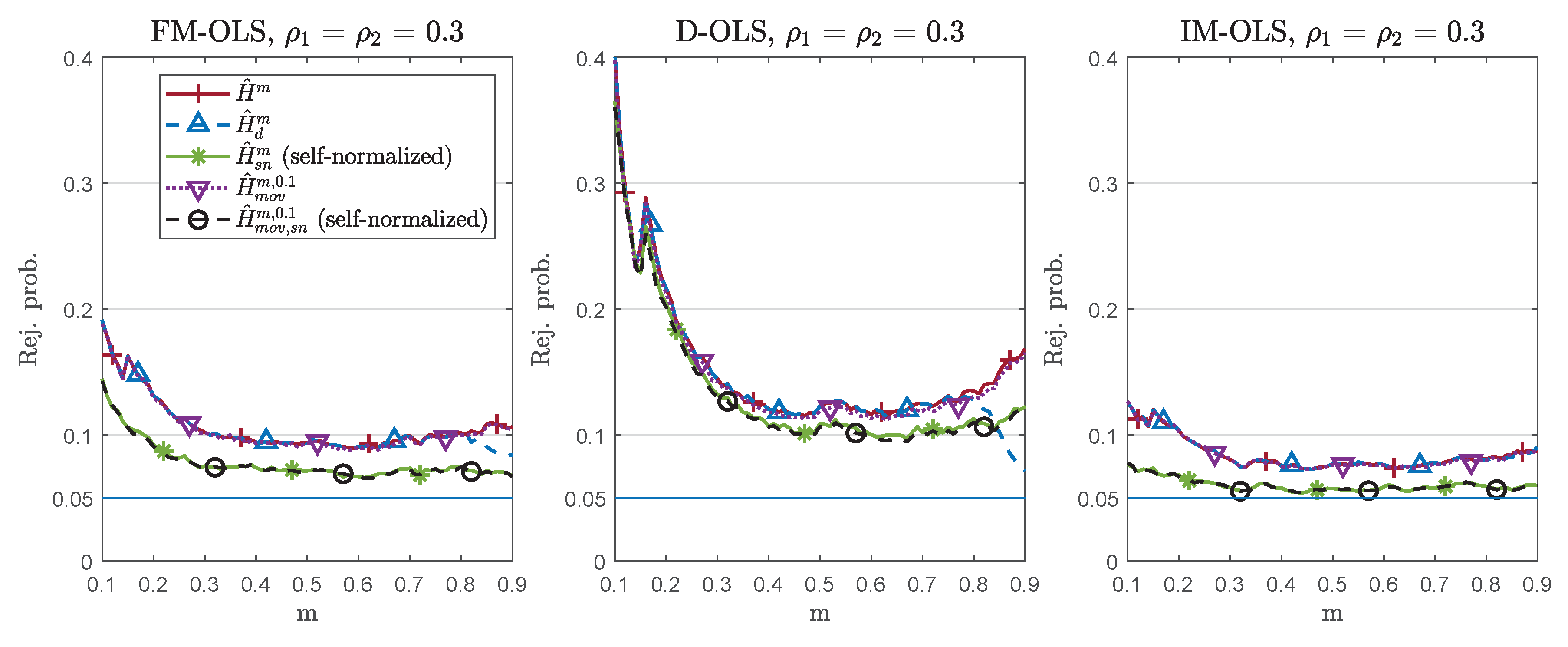
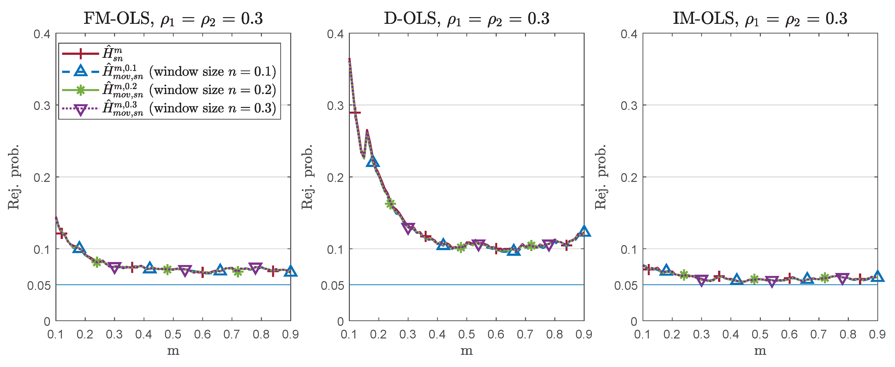
| 25. | The null rejection probability differences between the standardized and self-normalized detectors increase with increasing . The null rejection probability results for are contained in Figures S8 and S9 in Supplementary Appendix C. As expected, over-rejections are smaller than for , especially for small values of m, and the differences between the detectors also decrease. |
| 26. | Figure S10 in Supplementary Appendix C displays the corresponding results for . |
| 27. | We focus on size-corrected power because of the potential over-rejection problems under the null hypothesis. This allows us to see power differences across detectors while holding null rejection probabilities constant at 0.05. Clearly, this is useful for theoretical power comparisons, but it has to be kept in mind that such size-corrections are not feasible in practice. |
| 28. | See Figures S11 to S19 in Supplementary Appendix C for size-corrected power results in case of trend and slope breaks. |
| 29. | Table S1 in Supplementary Appendix C displays the corresponding size-corrected power results for . In addition, Tables S2 to S7 in Supplementary Appendix C display the results for for both and . |
| 30. | The main motivation for developing IM-OLS in Vogelsang and Wagner (2014a) was to develop an estimator that allows to perform fixed-b inference, which is an alternative asymptotic theory that captures the impact of kernel and bandwidth choices. These aspects are not covered by standard asymptotic theory. |
| 31. | Figure S20 in Supplementary Appendix C displays the corresponding detection times results for . |
| 32. | Only for twelve of these 18 countries, as discussed below, is the unit root null hypothesis not rejected for the logarithm of real per capita GDP. This, of course, reduces the number of countries for which monitoring is performed in this section to twelve countries. |
| 33. | Note that the combination of these two data sources using growth rates rests upon the assumption that the share of SO in SO is constant at about 98% also over the period 2006 onwards, as the OECD data comprise all SO emissions and not only SO emissions. |
| 34. | In addition, and preceding the oil price shock, many countries have put more stringent environmental legislation in place in the late 1960s or early 1970s, e.g., the United States introduced Clean Air Acts in 1963 and 1970, Canada introduced a similarly named law 1971, and Sweden introduced its Environmental Protection Act in 1969. |
| 35. | The detailed unit root test results using both the augmented Dickey-Fuller and the Phillips and Perron (1988) tests are contained in Supplementary Appendix D, Table S8, for the calibration period, and in Table S9 for the full sample period. With the exception of Germany and the augmented Dickey-Fuller test, and Austria, Germany, and New Zealand and the Phillips-Perron test, the unit root null hypothesis is not rejected over the full sample period. Thus, for the full sample period, the evidence for I(1) behavior of log real per capita GDP is, as expected, much stronger. We could, in principle, also consider a larger set of countries in the subsequent analysis, based on the probably more precise unit root test results obtained from a longer period. Zooming in a bit more by using a modified Phillips-Perron test of Perron and Vogelsang (1993) leads, e.g., for Austria to a non-rejection of the unit root null hypothesis when allowing for breaks in the intercept and trend slopes. Investigating such issues further, i.e., allowing for breaks in the regressors, is, despite its importance, beyond the scope of the present paper. As mentioned in Section 2.1, polynomial transformations of integrated processes are not integrated processes. Consequently, we do not perform unit root tests for the log per capita emissions series. Only in cases where a linear cointegrating relationship prevails (see Table 3) could we perform unit root tests also for the log per capita emissions series. |
| 36. | For linear cointegration, we also consider the Johansen (1995) test, in addition to the Shin (1994) test. For the higher order polynomial degrees, we use the extension discussed in Wagner and Hong (2016) or Wagner (2020). The detailed test results are available in Tables S10 and S11 in Supplementary Appendix D. |
| 37. | It is probably a philosophical question whether we observe in these cases a “straight-looking” line segment of an actually inverted U-type relationship or “really” a linear relationship. From an econometric perspective, the evidence is in favor of a linear relationship in a number of countries, and it, thus, is an interesting question to detect and date structural breaks based on monitoring a cointegrating linear relationship. We could alternatively also monitor for these countries, e.g., over-specified cubic relationships, where we would be also bound to find structural change for those countries where the data after the calibration period are changing from a linear towards an inverted U-shaped CPR relationship with a polynomial degree larger than one. |
| 38. | The full sets of results, including detection times for all detectors and estimators, are available in Supplementary Appendix D, in Table S15 for CO emissions, and in Table S16 for SO emissions. Given the performance advantages of FM-OLS over D-OLS, we exclude the D-OLS results from the discussion in the main text and discuss only FM-OLS and IM-OLS results here. |
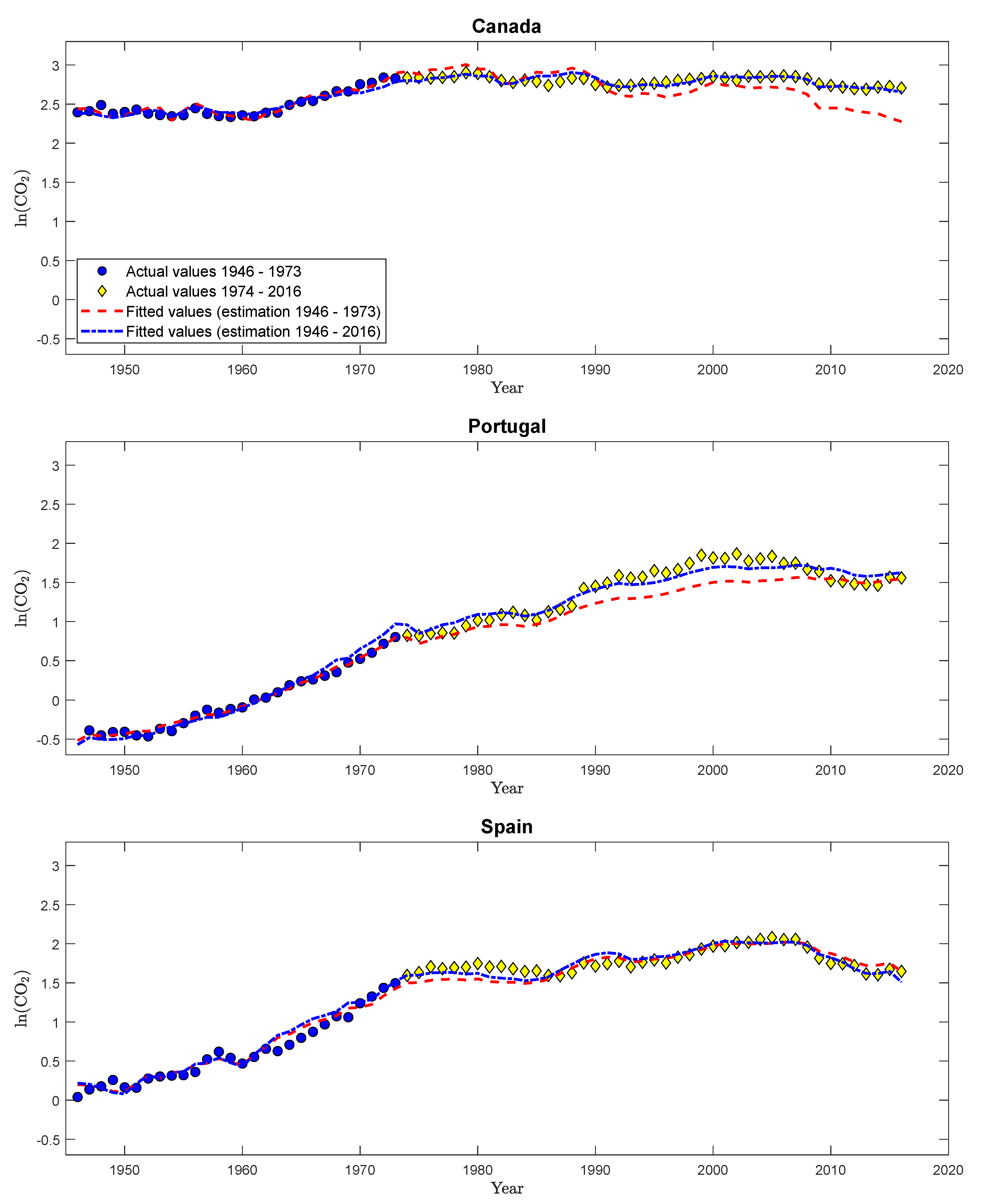
| 39. | Considering a quadratic specification over the full sample period, see Table S17 in Supplementary Appendix D for details, confirms this. For all countries, except Canada, Portugal, and Spain, the coefficients to log per capita GDP squared are (significantly) negative, whereas they show a positive sign for these three countries. The coefficient is, however, only significantly positive for Portugal, underlining the “borderline case” behavior of Portugal. |
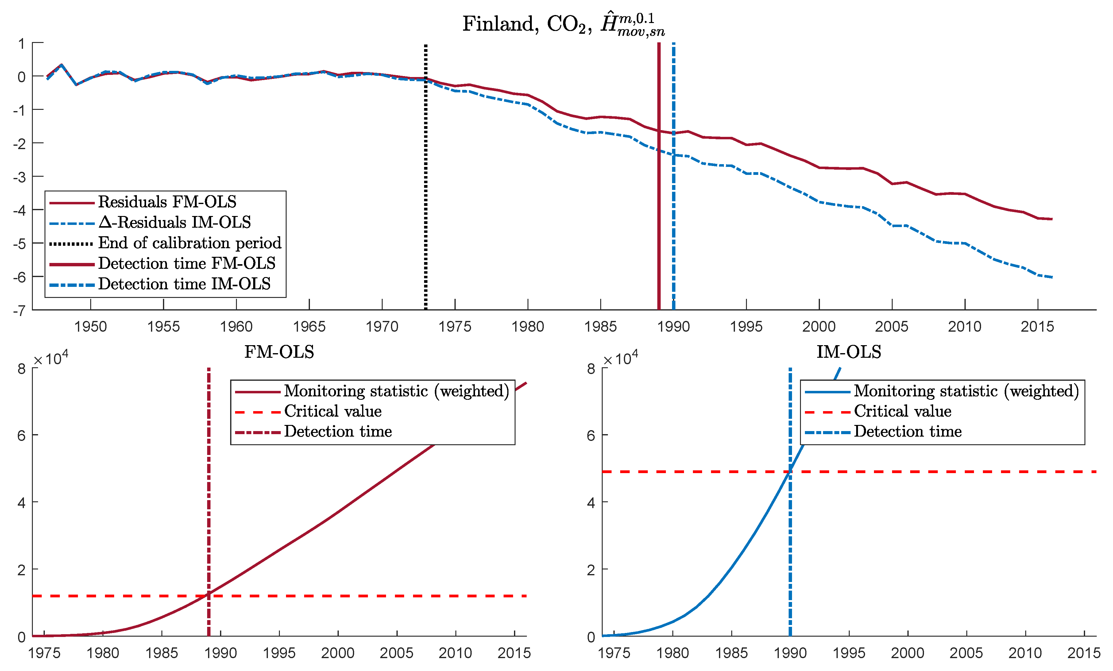
| 40. | Figures S32 to S42 in Supplementary Appendix D display monitoring results for CO2 emissions for the other eleven countries in exactly the same format as Figure 5 for Finland. |
| 41. | See Figure S29 in Supplementary Appendix D for analogous—and very similar—IM-OLS results. |
| 42. | Clearly, this is a long delay—particularly when looking at Figure 6, but it has to be taken into account that the estimation sample comprises only 28 observations, which is an rather small sample for cointegration analysis. |
| 43. | This appears to be the case indeed. The coefficients to squared log per capita GDP are very small but positive and borderline significant when estimated over the calibration sample (results are available upon request) and are significantly negative when estimated over the full sample (see Table S17 in Supplementary Appendix D). |
| 44. | Figure S30 in Supplementary Appendix D shows the corresponding results obtained with IM-OLS. |
| 45. | Table S12 in Supplementary Appendix D contains similar results concerning the minimal polynomial degrees of a CPR relationship for the full sample period as Table 3 for the calibration period. |
| 46. | Figures S43 to S54 in Supplementary Appendix D display monitoring results for SO2 emissions, with residuals and monitoring statistics analogous to Figure 5 for CO2 emissions for Finland, for all twelve countries. |
| 47. | This finding again indicates the potential gains to be reaped by considering pooling, across countries, or pollutants or both. Compare Wagner et al. (2020) for a discussion of pooling issues and options in the context of EKC analysis. This suggests that a worthwhile extension to be considered could be combining Wagner et al. (2020) with the monitoring ideas pursued in this paper. Such an extension, beyond the scope of this paper, could potentially lead to smaller delays. |
| 48. | It is in all likelihood mere coincidence that the trend coefficients are of more or less same magnitude over both sample periods with, effectively, only the sign changing. |
| 49. | Figure S31 in Supplementary Appendix D shows similar results when using IM-OLS for parameter estimation. |
| 50. | See Table S12 in Supplementary Appendix D for the minimal polynomial degrees on the full sample. |


| r | |||||||||||||
|---|---|---|---|---|---|---|---|---|---|---|---|---|---|
| FM | 0.19 | 0.07 | 0.05 | 0.32 | 0.64 | 0.14 | 0.34 | 0.46 | 0.80 | ||||
| D | 0.13 | 0.06 | 0.05 | 0.30 | 0.59 | 0.11 | 0.34 | 0.46 | 0.76 | ||||
| IM | 0.09 | 0.06 | 0.05 | 0.26 | 0.47 | 0.07 | 0.32 | 0.41 | 0.66 | ||||
| FM | 0.19 | 0.07 | 0.05 | 0.32 | 0.64 | 0.14 | 0.33 | 0.45 | 0.79 | ||||
| D | 0.13 | 0.06 | 0.05 | 0.30 | 0.59 | 0.11 | 0.33 | 0.45 | 0.76 | ||||
| IM | 0.09 | 0.06 | 0.05 | 0.26 | 0.47 | 0.07 | 0.32 | 0.41 | 0.66 | ||||
| FM | 0.20 | 0.07 | 0.05 | 0.17 | 0.61 | 0.14 | 0.16 | 0.26 | 0.77 | ||||
| D | 0.14 | 0.06 | 0.05 | 0.20 | 0.56 | 0.11 | 0.19 | 0.30 | 0.73 | ||||
| IM | 0.11 | 0.05 | 0.05 | 0.19 | 0.49 | 0.08 | 0.21 | 0.31 | 0.66 | ||||
| FM | 0.18 | 0.07 | 0.05 | 0.32 | 0.66 | 0.17 | 0.34 | 0.46 | 0.80 | ||||
| D | 0.12 | 0.06 | 0.05 | 0.29 | 0.61 | 0.13 | 0.34 | 0.46 | 0.77 | ||||
| IM | 0.09 | 0.05 | 0.05 | 0.25 | 0.48 | 0.09 | 0.31 | 0.40 | 0.67 | ||||
| FM | 0.18 | 0.07 | 0.05 | 0.32 | 0.65 | 0.15 | 0.34 | 0.46 | 0.80 | ||||
| D | 0.13 | 0.06 | 0.05 | 0.30 | 0.60 | 0.12 | 0.34 | 0.46 | 0.76 | ||||
| IM | 0.09 | 0.06 | 0.05 | 0.26 | 0.48 | 0.08 | 0.32 | 0.41 | 0.66 | ||||
| FM | 0.18 | 0.07 | 0.05 | 0.32 | 0.64 | 0.14 | 0.34 | 0.46 | 0.80 | ||||
| D | 0.13 | 0.06 | 0.05 | 0.30 | 0.59 | 0.11 | 0.34 | 0.46 | 0.76 | ||||
| IM | 0.09 | 0.06 | 0.05 | 0.26 | 0.47 | 0.08 | 0.32 | 0.41 | 0.66 | ||||
| FM | 0.20 | 0.07 | 0.05 | 0.17 | 0.63 | 0.18 | 0.16 | 0.26 | 0.77 | ||||
| D | 0.14 | 0.06 | 0.05 | 0.20 | 0.58 | 0.13 | 0.20 | 0.30 | 0.74 | ||||
| IM | 0.10 | 0.05 | 0.05 | 0.18 | 0.49 | 0.10 | 0.20 | 0.30 | 0.66 | ||||
| FM | 0.20 | 0.07 | 0.05 | 0.17 | 0.62 | 0.15 | 0.16 | 0.26 | 0.77 | ||||
| D | 0.14 | 0.06 | 0.05 | 0.20 | 0.57 | 0.11 | 0.19 | 0.30 | 0.73 | ||||
| IM | 0.10 | 0.05 | 0.05 | 0.19 | 0.49 | 0.09 | 0.21 | 0.31 | 0.66 | ||||
| FM | 0.20 | 0.07 | 0.05 | 0.17 | 0.62 | 0.14 | 0.16 | 0.26 | 0.77 | ||||
| D | 0.14 | 0.06 | 0.05 | 0.20 | 0.56 | 0.11 | 0.19 | 0.30 | 0.73 | ||||
| IM | 0.10 | 0.05 | 0.05 | 0.19 | 0.49 | 0.08 | 0.21 | 0.31 | 0.66 | ||||
| Australia | Austria | Belgium | Canada | Denmark | Finland |
| France | Germany | Italy | Japan | New Zealand | Norway |
| Portugal | Spain | Sweden | Switzerland | United Kingdom | United States |
| Polynomial Degree | ||
|---|---|---|
| Country | CO2 | SO2 |
| Australia | 1 | 1 |
| Belgium | 1 | 1 |
| Canada | 1 | 1 |
| Denmark | 1 | 2 |
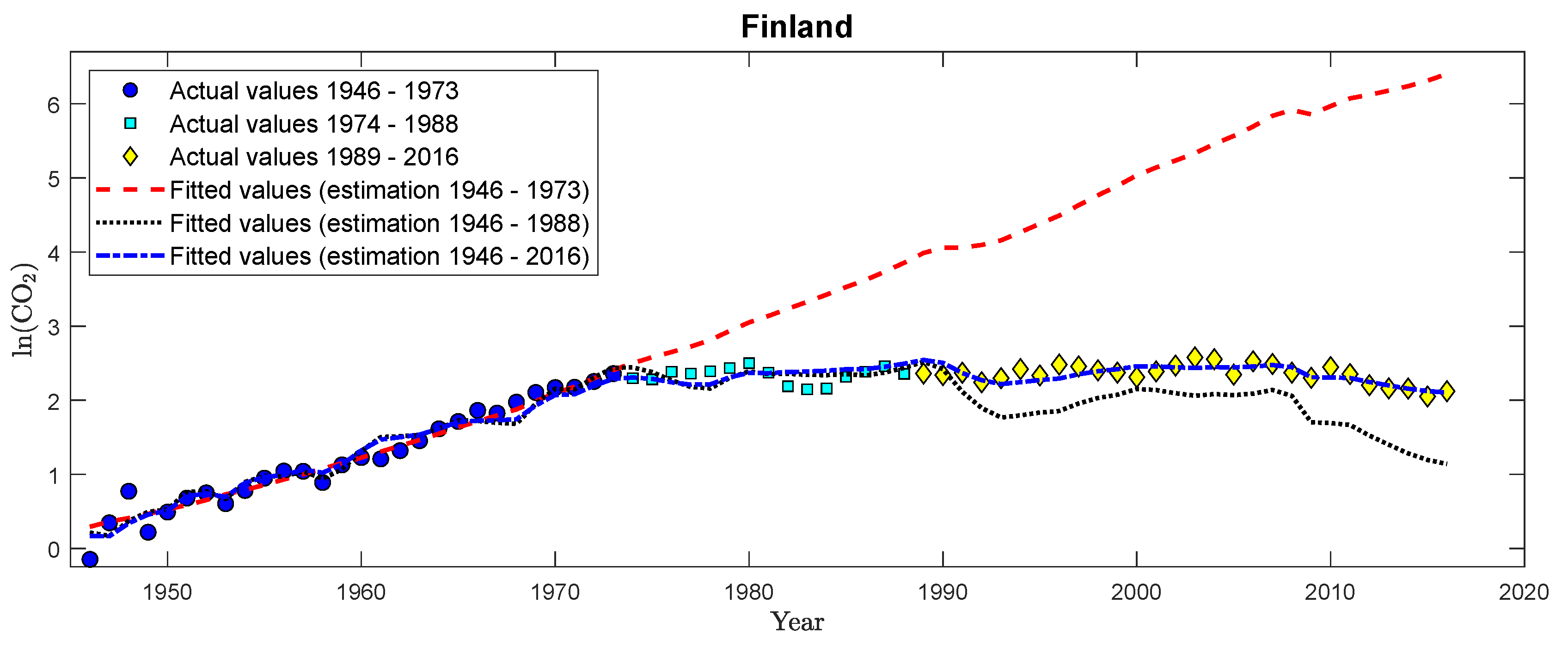
| Finland | 2 | 2 |
| Italy | 1 | 1 |
| Japan | 1 | 2 |
| Portugal | 1 | 1 |
| Spain | 1 | 1 |
| Sweden | 1 | 2 |
| United Kingdom | 1 | 1 |
| United States | 2 | 3 |
| Country | p | ||
|---|---|---|---|
| FM-OLS | IM-OLS | ||
| Australia | 1 | 1993 | 2001 |
| Belgium | 1 | 1988 | 1992 |
| Canada | 1 | ∞ | ∞ |
| Denmark | 1 | 1991 | 2011 |
| Finland | 2 | 1989 | 1990 |
| Italy | 1 | 1981 | 1982 |
| Japan | 1 | 1982 | 1980 |
| Portugal | 1 | 1998 | ∞ |
| Spain | 1 | ∞ | ∞ |
| Sweden | 1 | 1982 | 1983 |
| United Kingdom | 1 | 1984 | 1987 |
| United States | 2 | 1988 | 1992 |
| 1946–1973 | 1946–2016 | |||
|---|---|---|---|---|
| Canada | ||||
| FM-OLS | −0.056 | 2.841 | −0.027 | 1.661 |
| IM-OLS | −0.059 | 2.990 | −0.028 | 1.714 |
| Portugal | ||||
| FM-OLS | 0.000 | 1.003 | −0.008 | 1.341 |
| IM-OLS | 0.008 | 0.869 | 0.001 | 1.156 |
| Spain | ||||
| FM-OLS | −0.023 | 1.519 | −0.033 | 1.818 |
| IM-OLS | −0.039 | 1.789 | −0.036 | 1.911 |
| Country | p | ||
|---|---|---|---|
| FM-OLS | IM-OLS | ||
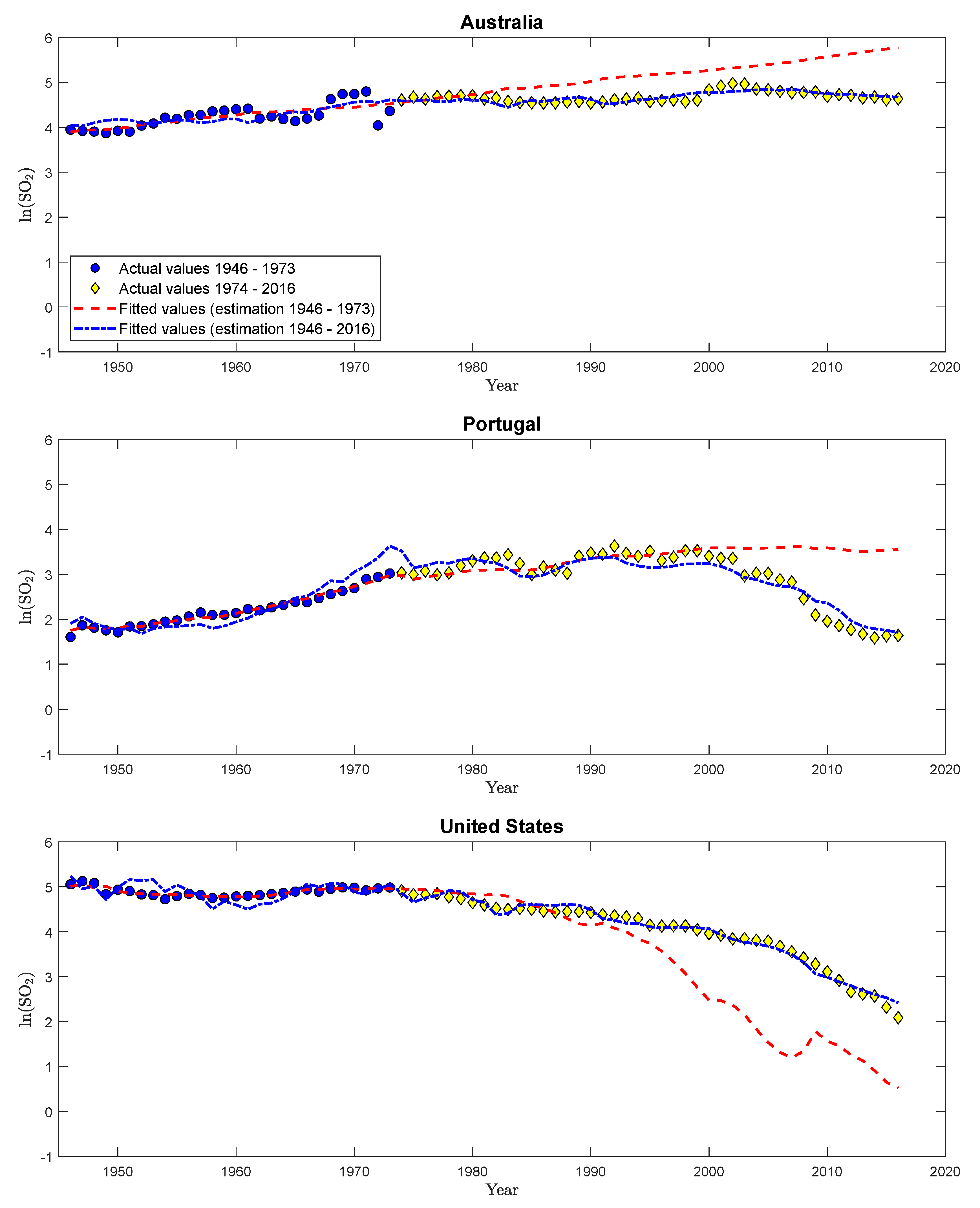
| Australia | 1 | ∞ | ∞ |
| Belgium | 1 | 1985 | 1985 |
| Canada | 1 | 1980 | 1981 |
| Denmark | 2 | 1997 | 2006 |
| Finland | 2 | 1988 | 1991 |
| Italy | 1 | 1982 | 1982 |
| Japan | 2 | 1991 | 2004 |
| Portugal | 1 | 2015 | ∞ |
| Spain | 1 | 2005 | 2012 |
| Sweden | 2 | 1985 | 1988 |
| United Kingdom | 1 | 1983 | 1983 |
| United States | 3 | ∞ | ∞ |
| 1946–1973 | 1946–2016 | ||||||||
|---|---|---|---|---|---|---|---|---|---|
| Australia | |||||||||
| FM-OLS | 0.043 | −0.819 | −0.042 | 2.541 | |||||
| IM-OLS | 0.042 | −0.770 | −0.043 | 2.550 | |||||
| Portugal | |||||||||
| FM-OLS | −0.005 | 1.047 | −0.104 | 3.491 | |||||
| IM-OLS | 0.002 | 0.873 | −0.092 | 3.215 | |||||
| United States | |||||||||
| FM-OLS | −0.013 | −1,831.120 | 183.982 | −6.158 | −0.133 | −305.981 | 31.361 | −1.052 | |
| IM-OLS | −0.005 | −2,190.198 | 220.246 | −7.380 | −0.133 | −61.963 | 7.512 | −0.275 | |
Publisher’s Note: MDPI stays neutral with regard to jurisdictional claims in published maps and institutional affiliations. |
© 2021 by the authors. Licensee MDPI, Basel, Switzerland. This article is an open access article distributed under the terms and conditions of the Creative Commons Attribution (CC BY) license (http://creativecommons.org/licenses/by/4.0/).
Share and Cite
Knorre, F.; Wagner, M.; Grupe, M. Monitoring Cointegrating Polynomial Regressions: Theory and Application to the Environmental Kuznets Curves for Carbon and Sulfur Dioxide Emissions. Econometrics 2021, 9, 12. https://0-doi-org.brum.beds.ac.uk/10.3390/econometrics9010012
Knorre F, Wagner M, Grupe M. Monitoring Cointegrating Polynomial Regressions: Theory and Application to the Environmental Kuznets Curves for Carbon and Sulfur Dioxide Emissions. Econometrics. 2021; 9(1):12. https://0-doi-org.brum.beds.ac.uk/10.3390/econometrics9010012
Chicago/Turabian StyleKnorre, Fabian, Martin Wagner, and Maximilian Grupe. 2021. "Monitoring Cointegrating Polynomial Regressions: Theory and Application to the Environmental Kuznets Curves for Carbon and Sulfur Dioxide Emissions" Econometrics 9, no. 1: 12. https://0-doi-org.brum.beds.ac.uk/10.3390/econometrics9010012