Enhanced Methods of Seasonal Adjustment

Department of Economics, University of Leciceter, Leciceter LE1 7RH, UK
Econometrics 2021, 9(1), 3; https://0-doi-org.brum.beds.ac.uk/10.3390/econometrics9010003
Submission received: 29 September 2020
/
Revised: 20 December 2020
/
Accepted: 24 December 2020
/
Published: 5 January 2021
(This article belongs to the Special Issue Topics in Computational Econometrics and Finance: Theory and Applications)
Abstract
:The effect of the conventional model-based methods of seasonal adjustment is to nullify the elements of the data that reside at the seasonal frequencies and to attenuate the elements at the adjacent frequencies. It may be desirable to nullify some of the adjacent elements instead of merely attenuating them. For this purpose, two alternative sets of procedures are presented that have been implemented in a computer program named SEASCAPE. In the first set of procedures, a basic seasonal adjustment filter is augmented by additional filters that are targeted at the adjacent frequencies. In the second set of procedures, a Fourier transform of the data is exploited to allow the elements in the vicinities of the seasonal frequencies to be eliminated or attenuated at will. The question is raised of whether an estimated trend-cycle trajectory that is devoid of high-frequency noise can serve in place of the seasonally adjusted data.
1. Introduction
This paper discusses some existing and some newly proposed methods for the seasonal adjustment of economic data. The new methods have been realised in the program SEASCAPE, which is available, together with a manual and a collection of data, at the following address: http://www.sigmapi.org.uk/seascape.zip/ (Supplementary Materials).
Two sets of methods are used preponderantly, at present, by central statistical offices. These are the heuristic methods that comprise the venerable X-11 procedure of Shiskin et al. (1967) and its derivatives and the newer model-based methods that are represented, primarily, by the TRAMO-SEATS package of Augustin Maravall. See Gómez and Maravall (1997, 2001) and Caporello and Maravall (2004). An alternative model-based approach approach to the structural analysis and prediction of time series is provided by the STAMP package of Koopman et al. (1995). A broad perspective on model-based business-cycle analysis and seasonal adjustment was provided by Kaiser and Maravall (2001).
The methods of TRAMO-SEATS and those of the current programs of the U.S. Bureau of the Census, designated as X-12ARIMA and X-13ARIMA-SEATS, which are the successors of X11, have been been re-engineered using an object-oriented approach and incorporated into the JDemetra+ program. (See Grudkowska 2017). This program has been officially recommended by European System of Central Banks (see Mazzi et al. 2018).
Both sets of methods operate in the time domain. They are complicated and difficult to master, albeit that they are accompanied, nowadays, by substantial manuals and by helpful online guidance. The X-11 program is well served by the monograph of Ladiray and Quenneville (2001).
The X-11 program was informed by a limited theory of filtering, which can be improved on. The model-based methods, which have been displacing X-11 and its derivatives, are the products of a dominant opinion amongst economists that economic investigations should be conducted within the context of well-defined models of economic activities.
A difficulty that can arise with models with parameters that are fixed over time is that they are sometimes incapable of capturing the complexities of the economic data. They can lead to distorted views of economic reality and to other failures when the models cannot be fitted adequately to the data. This may happen when the data are too heterogenous to sustain a model with fixed parameters.
Another problem that affects the time-domain methods of seasonal adjustment is that they nullify completely only the elements at the seasonal frequency and its harmonics. The seasonal fluctuations may comprise elements at adjacent frequencies that also need to be removed from the data.
A testimony to this problem was provided by McElroy and Roy (2017), who devised a means of detecting residual seasonal effects in seasonally adjusted data. The issue was also raised by Findley et al. (2005). The present paper describes some alternative means of addressing the problem that operate in the time domain and in the frequency domain.
The problems that can arise with the current time-domain methods of seasonal adjustment can be overcome either by augmenting them with additional filters or by forsaking them in favour of methods that operate in the frequency domain.
The purpose to which this paper testifies has been to build a program, called SEASCAPE, that comprises both some amended versions of the time-domain procedures and a full set of frequency-domain procedures. This should enable the two sets of procedures to be compared. However, it should be emphasised that there is no intention to prescribe a definitive method of seasonal adjustment. Instead, the purpose is to supplement the currently available methods.
2. The Structure of the Paper
The paper treats the time-domain methods and the frequency-domain methods of seasonal adjustment in succession.
The time-domain methods of this paper effect a twofold decomposition of the data into a seasonal component and a seasonally-adjusted data sequence; albeit that, in the case of the basic filter, there is also a provision for estimating a trend-cycle function.
The frequency-domain methods can effect either a twofold decomposition or a threefold decomposition. The latter comprises the seasonal component, a smooth trend-cycle function and a residual noise sequence.
The following five sections of the paper are devoted to the time-domain methods and the three subsequent sections are devoted to the frequency-domain methods. The disparity in the length of these two parts is a testimony to the greater complexity of the time-domain methods.
Section 3 describes the structure of a comb filter, which is a fundamental component of seasonal-adjustment filters operating in the time domain, albeit one that is sometimes well concealed. Section 4 and Section 5 derive an appropriate Wiener–Kolmogorov filter, described as the basic time-domain filter. The filter is derived, initially, in reference to a doubly-infinite data sequence. Then, it is adapted to data sequences that are finite and trended.
It is usual, in econometric modelling, to attribute the trends to poles of unit value within an autoregressive operator and to remove a trend by taking differences of the data. The method of de-trending that is pursued in this paper and in the associated program relies on the estimation of a polynomial trend function.
The polynomial trend might be better described as a base-line function, in order to avoid the implication that it represents a proper depiction of the low-frequency trajectory of the data. That role can be taken by the trend-cycle function.
The polynomial de-trending allows the spectral structure of the seasonal components of the data to be discerned clearly from the periodogram of the residual deviations of the data from the trend. It is notable that the residual sequence from fitting a polynomial of degree p by least-squares regression contains the same information as the sequence of pth-order differences.
Section 6 tackles the matter of widening the stop bands of a time-domain filter to encompass elements that are adjacent to those at the seasonal frequencies. This is achieved by applying the basic filter twice or three times in succession. Section 7 compares the effects of the basic time-domain filter with those of a conventional model-based filter.
Section 8 provides a brief account of the methods of filtering in the frequency-domain, which are given equal weight in the SEASCAPE program with the time-domain methods. The advantage of operating in the frequency domain is that it allows a free choice of the form of the frequency response function of the filter.
The widths of the stop bands should be chosen in view of the periodogram of the de-trended data. The widths of the transition bands and the profiles of the transitions are also matters of choice. Section 9 describes four alternative profiles that might be adopted.
The next two sections present case studies that illustrate the methods of seasonal adjustment. Section 10 describes the application of the basic time-domain filter to a tractable data sequence in which the seasonal fluctuations appear to comprise only the elements at the seasonal frequencies. In Section 11, a frequency-domain filter is applied to a data sequence in which the seasonal fluctuations comprise elements that are adjacent to the seasonal frequencies. The stop bands of the filter are set to widths that encompass these elements.
The frequency-domain methods have the advantage that they are better able to eliminate such elements and to prevent them from leaking into the seasonally adjusted data. They are capable, if so desired, of closely mimicking the time-domain methods. However, given the absence of an underlying parametric model, they do not lend themselves readily to the conventional methods of hypothesis testing.
3. Comb Filters
Any time-domain procedure for seasonal adjustment must contain a component that acts in the manner of a comb filter (see Proakis and Manolakis (1996) for a description of a comb filter in a signal processing context).
This filter is a rational polynomial function of the lag operator, albeit that it can be represented as a ratio of two polynomials of which the argument is a complex number z. Thus, the comb filter is represented by
where and where denotes either a quarterly or a monthly frequency of observation. Here, the numerator polynomial contains zeros at the seasonal frequencies, which are . These are amongst the roots of the equation , which are the so-called roots of unity. (The zero at the angle is excluded).
The nullification of the seasonal elements of the data is achieved by the zeros of the filter. The effects of these zeros at other frequencies is limited by the presence of the poles of the filter that lie on the same axes or radii as the zeros and that are close to the unit circle. At frequencies that are remote from the seasonal frequencies, the effects of the poles and the zeros are largely cancelled.
The poles that accompany the zeros are provided by the solutions to the equation , where is close to unity. These are roots of the denominator polynomial of the filter. The poles take the values , which is to say that they lie on a circle in the complex plane of radius . Figure 1 depicts the poles and the zeros of the comb filter, albeit that, for graphical purposes, the argument z of the polynomials has been replaced by , to keep the poles within the unit circle.
The filter of Equation (1) is unidirectional and backward looking, such that the filtered values will be formed from past and present values of the data. Therefore, the filter will induce a phase shift or a time lag in the processed data.
To avoid such an effect, the filter must reach equally forwards and backwards in time. For this reason, it is appropriate to adopt a bidirectional filter of the form
Here, is a factor that is adjusted to ensure that the value of is unity when . Then, the filter will preserve the levels of the data.
The effect of the filter is revealed by its frequency response function, which shows the manner in which the filter modifies the amplitudes of the sinusoidal elements of which the data are composed. It is obtained by setting and by running from zero to the limiting frequency of . The frequency responses of the monthly comb filters with and are shown in Figure 2.
The expansion of the rational function of Equation (2) will give rise to a doubly-infinite sequence of coefficients. Therefore, the filter cannot be applied directly to a finite sequence of data, unless one is prepared to truncate the sequence of coefficients. Instead, the filter may be applied in two passes running through the data in opposite directions.
These processes can be represented by the equations
where is the z-transform of the data sequence , is an intermediate sequence, generated by the forward pass of the one-sided filter of Equation (1), and is the final filtered sequence resulting from the backwards pass of the filter. These are hypothetical sequences defined over a doubly-infinite set of indices. In practice, to initiate the forwards and backwards passes, it is necessary to supply some initial conditions, to be obtained by backcasting and forecasting the elements of and , respectively. Typically, a model is used for this purpose, although Wildi (2005) proposed a nonparametric approach employing the periodogram of the data.
4. Wiener–Kolmogorov Filters
A problem with the filter of Equation (2) is the manner in which the peaks of the frequency response function that lie between the seasonal frequencies are diminished. Ideally, they should reach values close to unity so that the non-seasonal elements of the data can be largely preserved. In addition, this filter offers little control over the width of the clefts that surround the seasonal frequencies.
These problems can be overcome by adopting a Wiener–Kolmogorov formulation that gives rise to the following filter, wherein the factor , which is the ratio of the sum of the coefficients of the denominator and of the numerator, is to ensure that there is unit gain at the zero frequency:
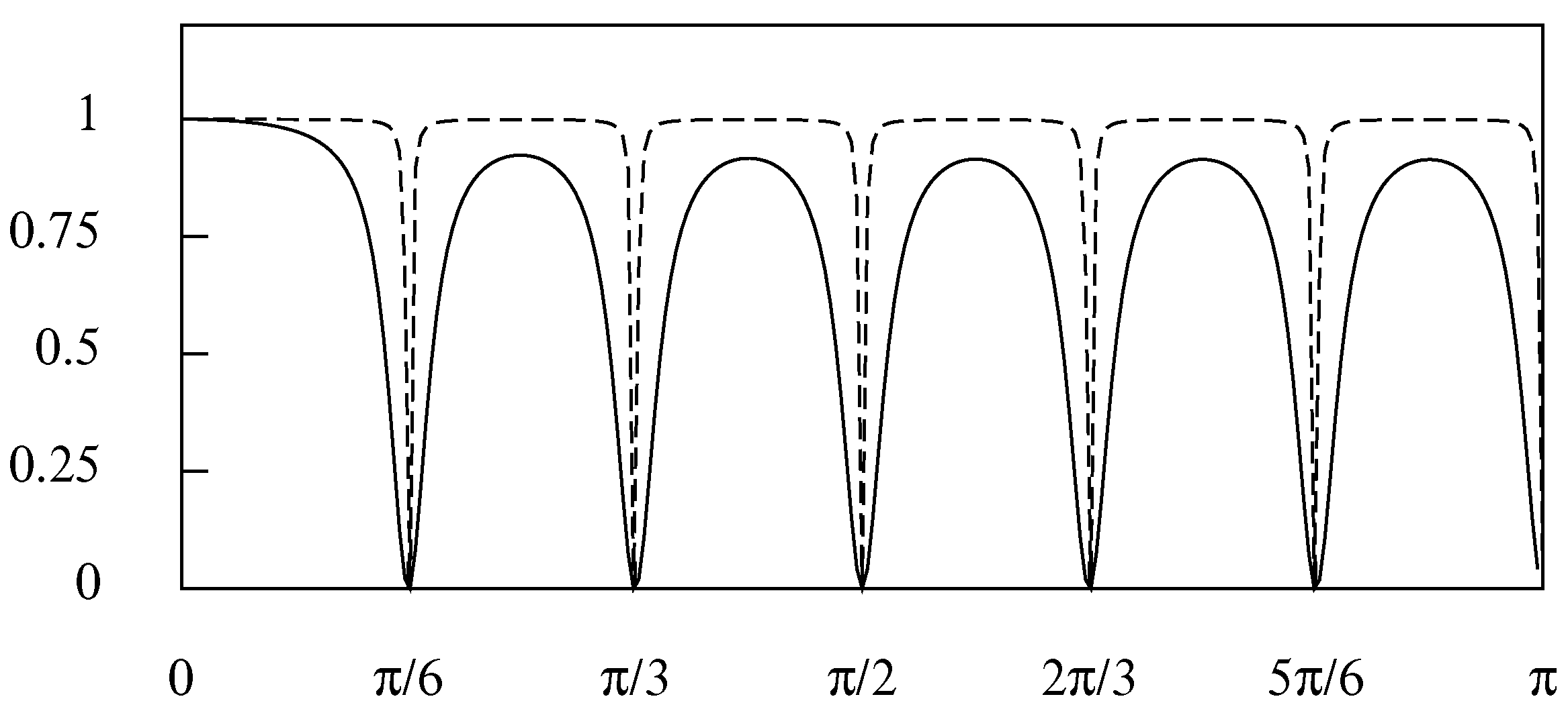
Figure 3 shows the frequency response function of two such filters, wherein the parameter values are and , which give rise to a frequency response function with narrow clefts at the seasonal frequencies, and and , which give rise to one with wide clefts.
The Wiener–Kolmogorov filters are commonly derived from statistical models that depict the logarithms of the data as a sum of statistically independent components:
Here, is a trend-cycle function, which can be decomposed into a polynomial trend and a cyclical function . The second term is a sequence of mean-zero seasonal fluctuations and the third term is a noise component, also of mean zero. The de-trended logarithmic data sequence that is devoid of the cyclical component may be denoted by .
An heuristic model that gives rise to the filter of Equation (4), albeit without the scaling factor , is represented in a z-transform notation by
where is the z-transform of the stochastic sequence and and are defined likewise. Both and stand for mutually independent white-noise processes with variances of and , respectively. (The model lacks the cyclical component , which can be deemed to have been absorbed within the noise component , if it has not been removed from in the process of de-trending the data).
It should be acknowledged that the z-transform of a stationary stochastic process, defined on a doubly-infinite set of integers, fails to converge anywhere in the complex plane. This difficulty can be overcome by truncating the sequence on both sides so that it has starting and ending points. In addition, the z-transform of is non-convergent in consequence of the unit roots of . This could be overcome by withdrawing the roots from the unit circle by an iota. Neither difficulty should impede the use of the z-transform in formal algebraic manipulations.
The presence of complex roots of unit modulus within the polynomial implies that the process is non-stationary in amplitude. It may be reduced to stationarity by multiplying throughout by to give
Under the assumption that the data have a normal distribution, or under the less stringent assumption that there is a linear regression relationship, the conditional expectation of given is
where E denotes the expectations operator, V is the variance operator and C is the covariance operator. Given that
and given that , it follows that
where . It will be recognised that is the ratio of the autocovariance generating functions of the and , which are stationary transforms of and , respectively. Equally, it is the ratio of the autocovariance generating function of and improper autocovariance generating function of the non-stationary sequence .
The scaling of the filter by in Equation (4), is in consequence of the fact that the seasonal component as modelled by Equation (6) is not zero-valued at the zero frequency, where . The estimate of the seasonal component will be obtained by subtracting the estimate of from .
To apply the filter in a bidirectional manner, it would be necessary to factorise the denominator as the product of a factor in z, to be used in the forwards pass, and a factor in , to be used in the backwards pass. Initial conditions for both processes would also need to be supplied. These difficulties can be overcome by adopting a genuine finite-sample version of the filter.
In deriving the seasonal component , the filter of Equation (4) could be applied equally to the residual deviations from a trend-cycle function or to the residuals from a polynomial regression. The results would be the same. This is explained by the fact that the polynomial trend and the trend-cycle component reside in intervals of the frequency spectrum that do not contain any of the elements of the seasonal component .
This outcome can be witnessed, in practice, in the context of the SEASCAPE computer program, which incorporates a variety of alternative de-trending procedures, operating in the time domain and in the frequency domain that can be applied to finite sequences.
In the twofold decomposition of , the seasonal component is extracted from the residuals of a polynomial regression, whereafter the seasonally adjusted data is obtained by subtraction.
In the threefold decomposition of , represented by Equation (5), the seasonal component is extracted from after the cyclical component has been extracted from the polynomial residuals and after has been formed. The residue of the extraction of from is the noise sequence .
However, within the time domain, the trend-cycle can be estimated directly by applying a Butterworth or a Hodrick–Prescott (Leser) filter to the trended data sequence , to create the sequence in one step, albeit that these filters can also be applied to in the manner described above. The Butterworth filter was described by Pollock (2000) and the Leser or Hodrick–Prescott filter was described by Leser (1961) and by Hodrick and Prescott (1997).
5. The Finite-Sample Wiener–Kolmogorov Filter
To derive the finite-sample version of the Wiener–Kolmogorov filter, consider a vector of T values drawn from the process represented by . In accordance with Equation (6), the vector may be decomposed as
The finite-sample version of the filter of Equation (10) will be a matrix transformation of order T that maps from the data vector y to a vector that represents the estimate of . To derive such a transformation, one can begin by finding the matrix analogues of the operators and .
These matrices can be obtained by replacing the argument z by the matrix lag operator of order T, which is derived from the identity matrix by deleting the leading column and by adding a column of zeros to the end of the array. The resulting matrices, denoted by and are lower-triangular. The matrices corresponding to and are the upper triangular matrices and , respectively.
It is notable that the first elements of would differ from the remaining elements in so far as they comprise fewer than s elements of the data vector. To supply the missing elements, some pre-sample values of the data might be generated.
An alternative recourse is to discard the first elements of the transformation. Consider the following equations:
The effect of discarding the subvectors and can be achieved by replacing and by and respectively. Then, the matrix analogue of the filter of Equation (4) becomes
The scaling factor continues to be used to ensure that the filter has unit gain at the zero frequency.
The unscaled filter can be derived from a conditional expectation. Applying to the equation , representing the seasonally fluctuating data, gives
This is just a segment of elements drawn from the process represented by Equation (7).
The expectations and the dispersion matrices of the component vectors of g are
where D is the operator that creates the variance–covariance or dispersion matrix.
The conditional expectation of , given the transformed data , is provided by the formula
where the second equality follows in view of the zero-valued expectations of and g. Within this expression, there are
Putting these details into Equation (16) gives the following estimate of :
where .
A simple procedure for calculating begins by solving the equation
for the value of b. Thereafter, one can generate .
The solution to Equation (19) may be found via a Cholesky factorisation that sets , where L is a lower-triangular matrix with a limited number of nonzero bands and D is a diagonal matrix. The system may be cast in the form of and solved for p. Then, can be solved for b, whence can be derived.
It will be observed that Equation (18) can also be written as
where is an upper-triangular matrix and its transpose is a lower-triangular matrix. This equation corresponds to a method of bi-directional filtering in which represents a real-time filtering and represent a reverse-time filtering, which is also described as a smoothing operation.
The transformations of Equations (13) and (18) entail a bi-symmetric matrix (which is symmetric with respect to both the NW–SE and the NE–SW diagonals). One consequence of this characteristic is that the outcome is invariant with respect to the reversal of the order of the element in the vector y. Thus, if the reversed vector is denoted by , where J is a matrix with units on the NE–SW diagonal and with zeros elsewhere, and if , then , where .
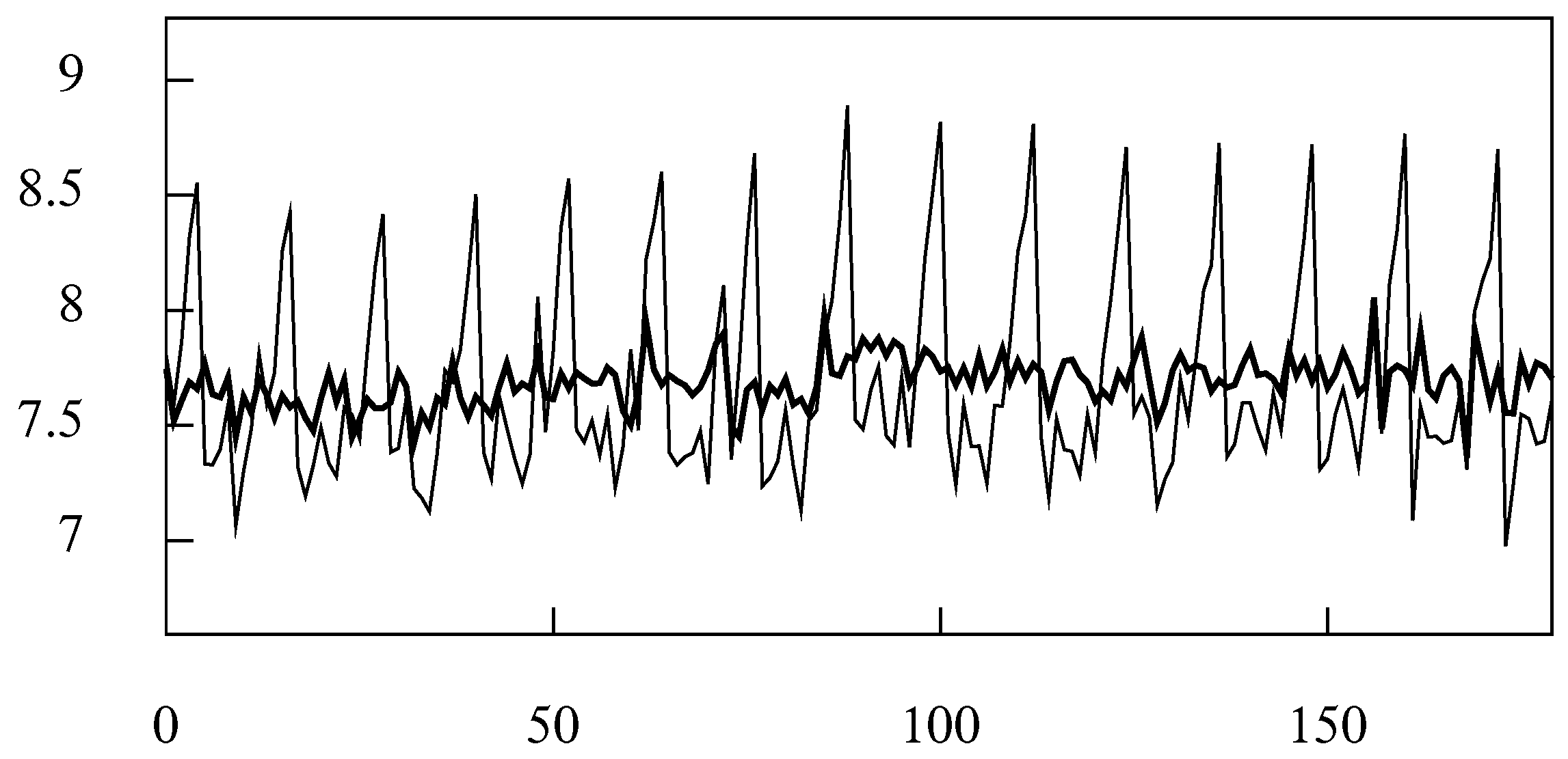
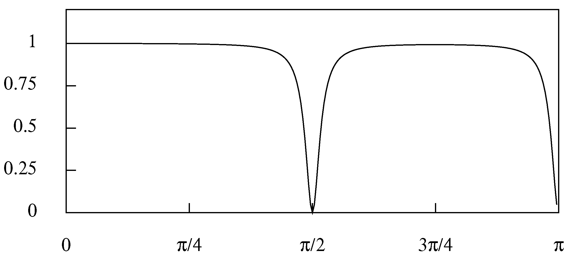
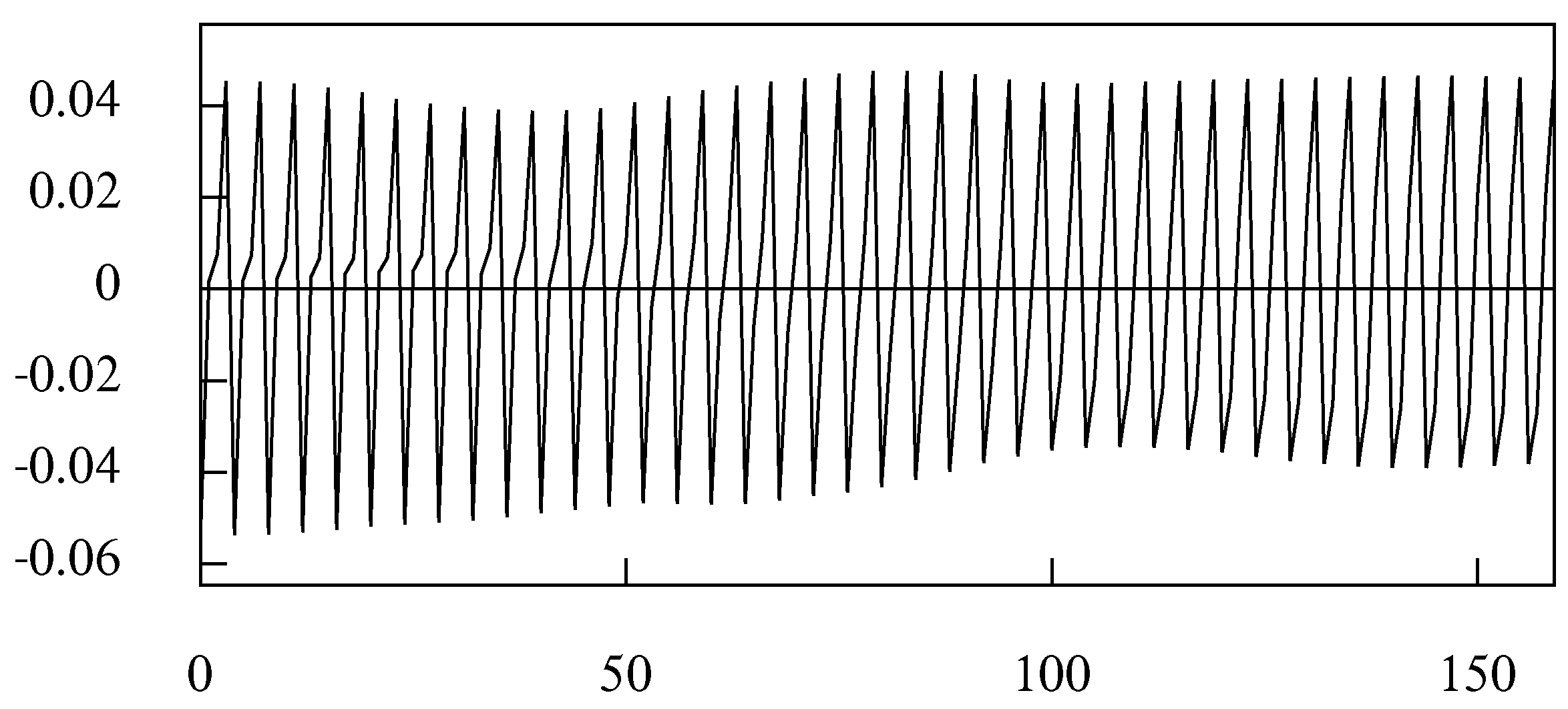
Figure 4 shows the frequency response function of the basic seasonal adjustment filter for quarterly data, which presupposes a doubly-infinite data sequence. Figure 5 shows the effect of applying the basic (finite-sample) quarterly seasonal-adjustment filter to the residuals from a linear de-trending of the logarithms of an index of quarterly U.K. consumption for 1955–1994. Figure 6 shows the seasonal component that has been extracted from these data.
The seasonally adjusted data of Figure 5, which correspond to , have a rough and irregular profile that contrasts markedly with the regularity of the seasonal component , shown in Figure 6. That regularity is unsurprising in view of the fact that the component extracted by the basic seasonal-adjustment filter comprises a restricted set of seasonal elements consisting only of those at the fundamental seasonal frequency and at its harmonic frequency, together with some severely attenuated elements at the adjacent frequencies.
One might wish for a smoother version for the trajectory of the seasonally-adjusted data. Such trajectories are shown in Figures 12 and 14, which become trend-cycle functions when they are added to the polynomial functions that have served to de-trend the data.
Within a threefold decomposition of the data , lying between the regular series of seasonal fluctuations and the smooth trend-cycle function , will be a rough and irregular sequence that is liable to be disregarded as noise, unless it shows some correlation with other economic variables or events.
A smooth trend-cycle function can be created also by applying the time-domain Butterworth filter directly to the data. The residual deviations of the data from the trend-cycle trajectory can be subjected to a seasonal adjustment procedure to create a seasonal component and a residual component, which is the putative noise.
6. Widening the Seasonal Stopbands
Figure 4 shows the frequency response function of the basic time-domain seasonal adjustment filter for quarterly data when the smoothing parameters is and the pole parameter is . There is a complete nullification of the elements at the seasonal frequencies; and those at the adjacent frequencies are attenuated to an extent that diminishes rapidly as their distance from the seasonal frequencies increases.
To increase the attenuation of the elements of the data that are adjacent to the seasonal frequencies, one can reduce the value of within the polynomial . This will draw the poles away from the unit circle, with an effect that can be seen by comparing the two functions that are plotted in Figure 3.
It may be required to impose a greater attenuation on the adjacent elements than can be achieved by reductions in the value of , and it may be desirable to confine this effect more narrowly to the vicinities of the seasonal frequencies.
For this purpose, it might be appropriate to apply the seasonal-adjustment filter twice or more times in succession and with poles and zeros that are displaced from the seasonal frequencies by small angles. A double filter with equal displacements on either side of the seasonal frequencies could take the form of
where is the angle of the displacement. It should be observed that . Thus, the same factor is present in both and . To avoid the duplication, it is reasonable to exclude the factor from the second of these filters.
Figure 7 shows the frequency response of the resulting double filter for monthly data in which the offsets are degrees (0.0349 radians). The lack of zeros at the seasonal frequencies allows a small amount of leakage to occur, which increases with the size of the offsets and with the value of . Given the likely prominence of the elements of the data at the seasonal frequencies, this leakage is liable to prove problematic.
To overcome the leakage of the double filter, it is possible to combine the basic filter with the two offset filters to create a triple filter. The basic filter will have its poles and zeros at exactly the seasonal frequencies. The second and third filters will have their poles and zeros offset to the left and right, respectively. Moreover, it may be desirable to chose individually the values of the offsets on either side of the seasonal frequencies.
Thus, if it is required to place additional poles and zeros on either side of the seasonal frequencies , then it becomes appropriate to compound the denominator polynomials of the offset filters from the factors
and to compound their numerator polynomials from similar factors, but with .
The appropriate displacements can be determined with reference to the periodogram of the seasonal data after their trend has been removed. This will indicate which of the data elements adjacent to the seasonal elements should be taken into account, to be eliminated or attenuated.
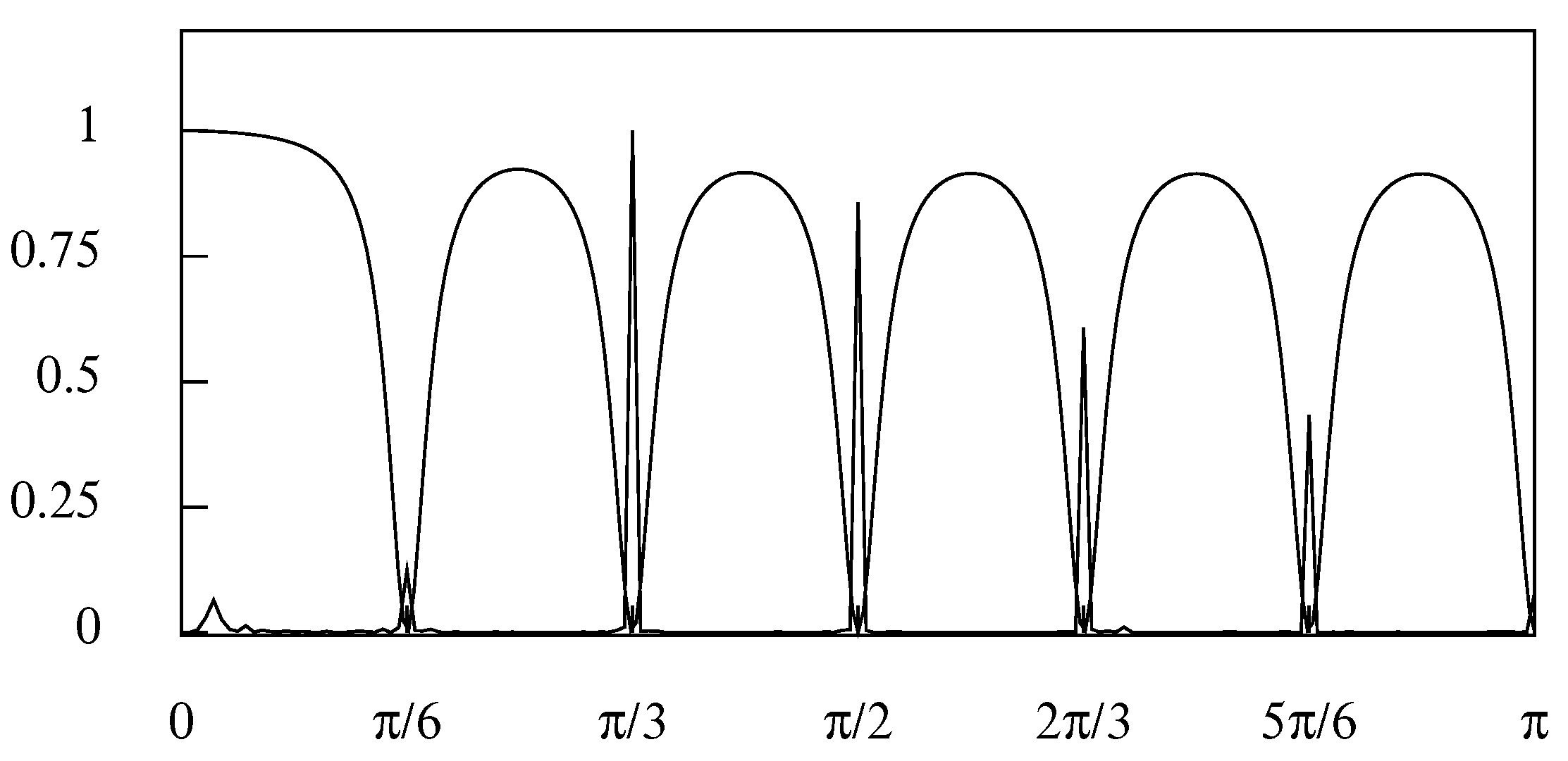
The frequency response of such a triple filter is illustrated in Figure 8. Here, the values of and , which have characterised the previous filters, are retained. However, an offset of three degrees (0.0524 radians) has been applied on either side of each of the seasonal frequencies.
A problem with the frequency response of the triple filter is that its values at the midpoints between the seasonal frequencies are significantly less that unity. This conflicts with the intention of preserving the elements of the data at these points and in the vicinities thereof. Moreover, there will be an uncomfortable degree of leakage in the stop bands of the filter when they become wide. A similar but a less severe attenuation of the amplitudes of the non-seasonal elements occurs with the double filter. Both of these problems can be overcome by operating in the frequency domain, as described in Section 8.
7. Time Domain Filters for Extracting the Trend-Cycle Function
The economic models that underlie the TRAMO-SEATS and STAMP programs contain explicit trend-cycle functions of the nature of second-order or integrated random walks. These functions give rise to filters that can be used to extract trend-cycle functions from the data, which are somewhat smoother than the seasonally adjusted data sequences.
In the seasonal adjustment procedures of the SEASCAPE program that work in the time domain, the trend is extracted by a polynomial regression. The regression residuals are then subjected to a seasonal adjustment filter, whereafter they are added back to the polynomial to create the seasonally adjusted data.
The trend extraction filters of the TRAMO-SEATS and STAMP programs can be mimicked, nevertheless, by applying a low pass smoothing filter to the seasonally adjusted residuals. When the resulting sequence is added to the polynomial trend, the result is similar to those obtained from the above-mentioned programs.
The procedures of the TRAMO-SEATS program are based, in the most common case, on the airline passenger model of Box and Jenkins (1976), which is represented by the equation
where is the twofold differencing operator, where and where is the z-transform of a white-noise forcing function. The parameter values estimated by Box and Jenkins, which are the values that determine the frequency response functions of Figure 9 and Figure 10, are and .
The program effects a decomposition of the data into a seasonal component, a trend-cycle component and a noise component, which are described by statistically independent processes driven by separate white-noise forcing functions. It espouses the principle of canonical decompositions that was expounded by Hillmer and Tiao (1982).
This principle proposes that any elements of white noise that are present in the seasonal component and the trend component, after an initial decomposition, should be extracted from them and assigned to the noise component. The filters for estimating the trend component and the seasonal component are derived according to the Wiener–Kolmogorov principle.
Thus, the filters can be derived from a meta-model defined by the equation
where , and represent mutually independent white-noise processes and and are polynomials with zeros on the unit circle such as to eliminate white-noise components from within the trend and the seasonal components. (The white-noise components have uniform spectra over the interval ).
Whereas no explicit expressions are available for and , the expressions for and were provided by Hillmer and Tiao (1982). On this basis, the trend-extraction filter can be represented by the equation
This is a ratio of the (improper) autocovariance generating functions of the trend component and of the data. The filter for extracting the seasonal component is constructed likewise. The seasonally adjusted sequence is created by subtracting the estimated seasonal component from the data sequence. Therefore, it may be regarded as a composite of the trend component and the noise component.
Figure 9 represents the frequency response function of the seasonal adjustment filter derived from the airline passenger model. It differs hardly from the frequency response function of Figure 3 derived from the heuristic model of Equation (6). Figure 10 represents the frequency response function of the trend (or trend-cycle) extraction filter derived from the airline passenger model.
To mimic the trend extraction filter of Figure 10, a binomial smoothing filter can be applied in series with the basic seasonal adjustment filter of Equation (13) to create a composite filter. The coefficients of the binomial filter are generated by the following recursion:
where n is an even number. The z-transform of the symmetric phase-neutral binomial filter is
The frequency response, which is obtained by setting , is
This result, which may seem remarkable, was demonstrated by Pollock (2018).
As n increases, the attenuation of the high frequency elements of the data increases, and the profile of frequency response of the binomial filter, defined over the interval , converges to the profile of a normal distribution. The frequency response function of the composite filter, derived by applying the binomial smoothing filter with in series with the basic filter monthly filter with and , is shown in Figure 11. The effect of applying the quarterly composite filter with the same parameters to the sequence of Figure 5 is shown in Figure 12. Here, the bold line represents the cyclical part of a putative trend-cycle function.
A disadvantage of the composite filter is that it is liable to transmit elements of noise that reside in the interstices between the seasonal frequencies, thereby adding roughness to the cycles. These cycles lack the smoothness and regularity of cycles that can be extracted by the alternative frequency-domain methods, such as those depicted in Figure 14. A low pass frequency-domain filter with a cut-off point that falls short of the fundamental seasonal frequency will not transmit noisy elements of higher frequencies.
8. The Frequency-Domain Methods
The methods of seasonal adjustment that operate in the frequency domain are more flexible than the conventional time-domain methods. The Fourier ordinates of a de-trended data sequence can be rescaled in any way that is deemed to be appropriate, thereby altering the amplitude of the sinusoidal elements of which the data are composed.
A close inspection of the periodogram of the de-trended data should indicate which of the elements need to removed or to be attenuated in pursuit of the seasonal adjustment. The effects of the irregularities of the calendar, and the effects of strikes and holidays etc. can induce irregularities in the seasonal fluctuations. Then, the fluctuations are liable to comprise elements at frequencies that are adjacent to the seasonal frequency and its harmonics, which can be removed from the data by operating in the frequency domain.
In the conventional methods of seasonal adjustment, such irregularities are addressed directly by adjusting the data. Descriptions of the methods were provided recently by Attal-Toubert et al. (2018) and Ladiray (2018). The methods are complicated, and they require expertise. It is possible that they could be avoided and that the irregularities could be accommodated by operating on the Fourier ordinates in the frequency domain.
The relationship between the data sequence and the Fourier ordinates is represented by
The first of these equations, which depicts the inverse Fourier transform, represents the Fourier synthesis of the data. The second equation, which depicts the direct Fourier transform, represents the analysis of the data.
The data can also be expressed in terms of a set of mutually orthogonal trigonometric functions:
where is the quotient (i.e. the integral part) of . The coefficients of this equation are
whereas, according to Euler’s equations, there are
The coefficients of Equation (30) are obtained by projecting the data onto the trigonometrical functions. In the case where T is an odd number, this gives
where . In the case where T is an even number, the formulae above are valid for , and, for , there are
In both cases, there is .
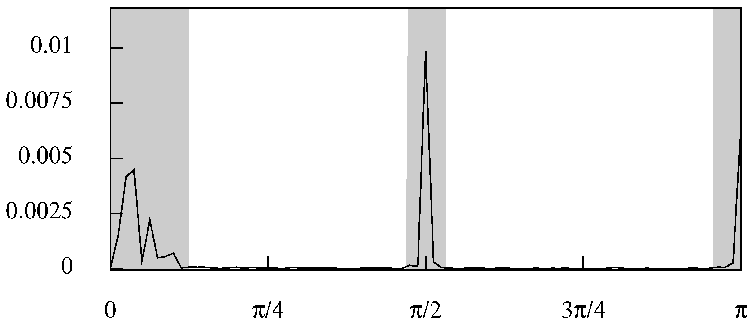
The periodogram of the data is the graph of the function . Figure 13 shows the periodogram of the consumption data that are portrayed in Figure 5 and Figure 12.
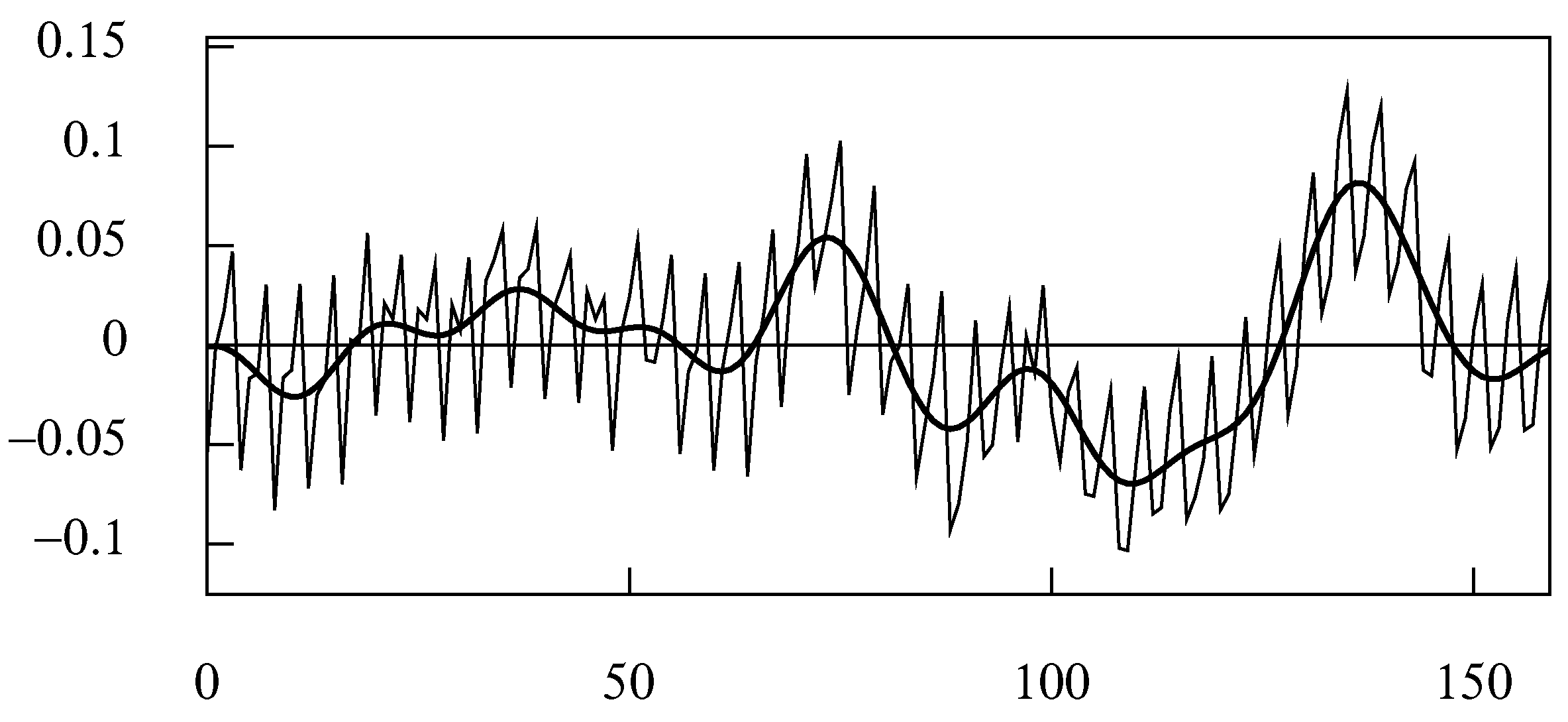
In this figure, the seasonal elements that it would be appropriate to remove from the data correspond to the highlighted bands in the vicinities of and . Apart from the spectral structure that falls within the frequency interval , there is little else in the data. Nevertheless, there is noise in the data that falls within the dead spaces that occupy the remainder of the frequency axis. Therefore, it is appropriate to represent the business cycle by a synthesis of the sinusoidal elements that lie in the interval . The result is represented in Figure 14.
This representation of the business cycle is liable to be preferred to that of Figure 12, which has been produced by a time-domain method and which is affected by some of the noise from within the dead spaces and by some proportion of the elements that are adjacent to the seasonal frequencies.
The difference between the smooth trajectory of Figure 14 and the rough seasonally adjusted sequence of Figure 5 appears to be only noise that is devoid of any economic information. Therefore, it can be argued that the estimated trend-cycle sequence of Figure 14 should serve for the seasonally adjusted data.
9. Stop Bands and Transition Bands
The advantage of the frequency-domain method of seasonal adjustment is that it allows complete flexibility in determining an appropriate frequency response for eliminating the seasonal effects from the data. The simplest design is one in which the stop bands, which eliminate the seasonal elements of the data, have zero gain and in which the pass bands that preserve all other elements have unit gain.
The extent of the stop bands, which cover the seasonal frequency and its harmonic frequencies, can be determined in the light of the periodogram of the de-trended data. The elements adjacent to those of the seasonal frequencies, which might be thought to contribute to the seasonal fluctuations, can also be covered by the stop bands, albeit that, alternatively, they can be partially attenuated within adjacent transition bands. In Figure 13, the clefts that surround the seasonal frequencies are vertical shafts, and there are no transition bands.
It is possible to define transition bands that allow a gradual transition between the pass bands and the stop bands. The trajectory of the frequency response within these bands must make a monotonic transition from unity to zero and vice versa; but, otherwise, its precise nature is a matter of choice. The SEASCAPE program offers four choices. The first choice, denoted no transitions, is to allow the frequency response to pass abruptly between unity and zero and vice versa.
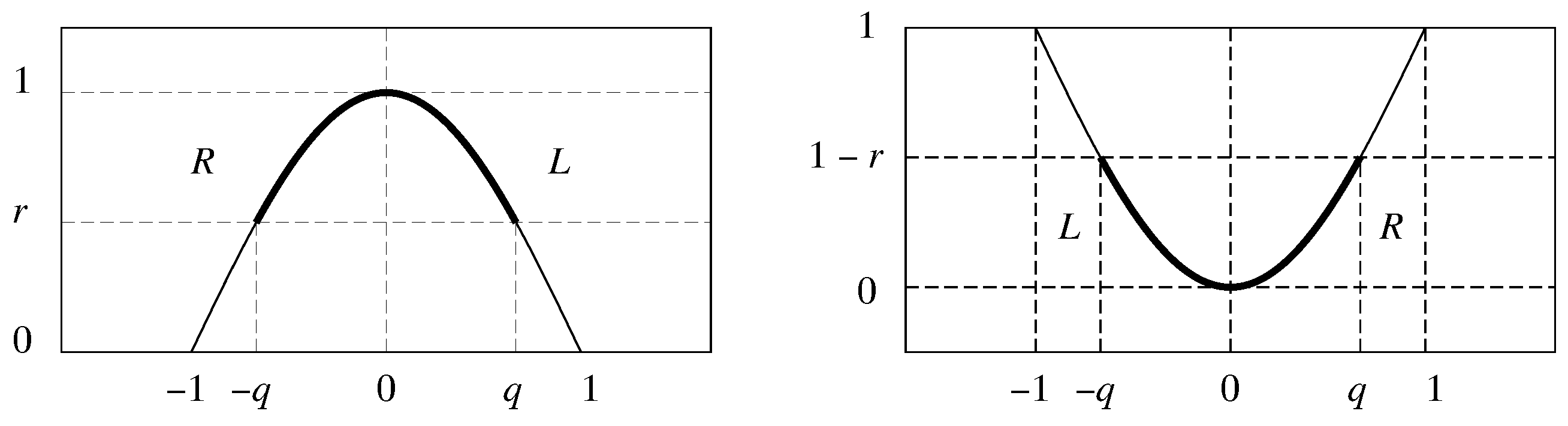
The second possibility, described as the upper-half cosine transitions, is to govern the transitions by segments of a cosine function of , where x is restricted to the intervals and . The transition on L (L for left or lower) from the pass band to the stop band occurs when and the transition on R (R for right or upper) from the stop band to the pass band occurs when . Thus, the upper-half cosine transitions are generated by the function
Here, is a parameter that adjusts the shape of the transitions by abbreviating them. The integer affects the curvature at the beginning of the transitions, which become more gradual as n increases, whereas the descent, or the ascent, which is delayed, becomes more rapid. The formulation of Equation (35) is readily intelligible when and . When , the formulation can be understood in the light of the left side of Figure 15.
The third choice, which is described as the lower-half cosine transitions, employs the function
Here, the transition L from pass band to stop band occur when and the transition R from the stop band to the pass band occurs when . The right side of Figure 15 elucidates this formulation.
To complete these specifications, there must be mappings from the frequency index to the variable x that governs frequency response within the clefts that comprise the transition bands and the stop bands. A sub-interval of on which a cleft is defined takes form of
where and are left and right transition bands, respectively, and is the stop band. Then, in the case of the upper-half cosine transitions of Equation (35), there are
whereas, in the case of the lower-half cosine transition of (36), there are
A fourth choice is to govern the transitions by a sigmoid or logistic function. There are numerous functions that might be employed, were it not for the fact that they tend to their asymptotes of unity and zero as . For present purposes, the sigmoid functions must reach their upper and lower levels at the boundaries of the transition regions. A flexible function that satisfies this requirement can be formed by joining the upper and lower cosine transition functions.
The left-side composite sigmoid function is defined as a function of comprising two segments as follows:
The segments join seamlessly when . The right-side function is obtained when is run in reverse.
If there is a requirement to mimic the effects of one of the time-domain filters, then it will be appropriate to employ the upper-half cosine transitions. An example is provided by the triple time-domain filter of which the frequency response is portrayed in Figure 8. The frequency response of a frequency-domain version of the filter is shown in Figure 16.
There are some manifest differences in the two frequency responses. The frequency-domain filter shows no leakage in the stop bands. The gain of the filter in the regions between the stop bands reaches unity, with the effect that the non-seasonal components are suffering from less attenuation than in the case of the time-domain filter. These features can be counted as advantages.
It is unclear why this filter should be preferred to one that makes abrupt transitions between the pass bands and the stop bands. However, an abrupt transition can induce persistent oscillations in the processed data, which correspond to the phenomenon of ringing in audio-acoustic processing. This will not be an issue when the transition occurs within a dead space of the periodogram, which is devoid elements of a significant magnitude.
The left-side composite function will serve for the transition band of a low pass filter. The right-side function will serve for the transition band of a high pass filter. Figure 17 shows, via the continuous line, the frequency response of a low pass filter. It shows, via the dashed line, the frequency response of the complementary high pass filter. The sum of the two frequency responses is unity, which implies that the complementary filters partition the data.
The low pass filter, of which the frequency response resembles that of the Butterworth filter, will serve to isolate a trend-cycle function. The rate of transition can be increased either by raising the value of n or by narrowing the transition band, or by both. For an account of the finite-sample Butterworth filter, see the article of Pollock (2000).
10. Case Study 1: The Basic Time-Domain Filter and the Trend-Cycle Function
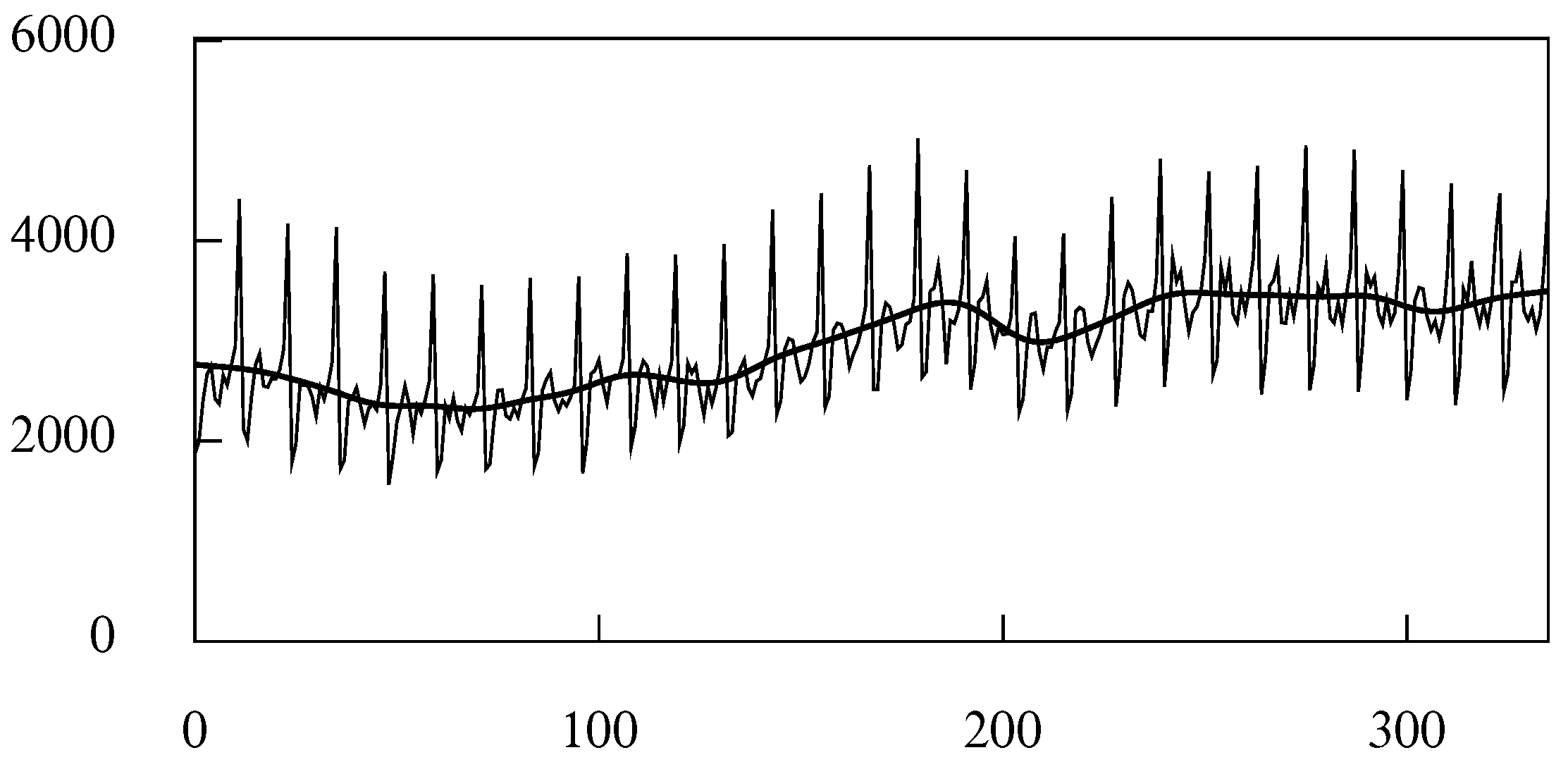
Figure 18 shows a set of 336 monthly observations of the value in US dollars of the sales of women’s clothing. Superimposed on the data is an interpolated polynomial function of degree 4, which serves as a preliminary representation of the trend. Figure 19 shows the periodogram of the residual deviations of the data from the polynomial trend together with the frequency response function of the basic time-domain seasonal adjustment filter. The narrow spikes of the periodogram suggest that the seasonal component comprises only the elements at the seasonal frequencies. Therefore, the basic filter should be sufficient for removing the seasonal fluctuations from the data. The seasonally adjusted data, which are formed by subtracting the seasonal component from the data are shown in Figure 20. Their trajectory has a rough profile.
The periodogram also bears the spectral signature of a low frequency cycle. The cycle can be extracted from the residuals and added to the polynomial to create the trend-cycle function.
The cycle has been extracted by a low pass Butterworth filter of order 6 and with a nominal cutoff point at , which exceeds the maximum frequency within the cycle. The resulting trend-cycle function is shown in Figure 21. This has a smooth profile. The difference between this trajectory and that of the seasonally adjusted data is a sequence that might be construed as noise devoid of information. In that case, one might prefer to use the trend-cycle function in place of the seasonally adjusted data.
11. Case Study 2: Widening the Stop Bands via the Frequency Domain Filter
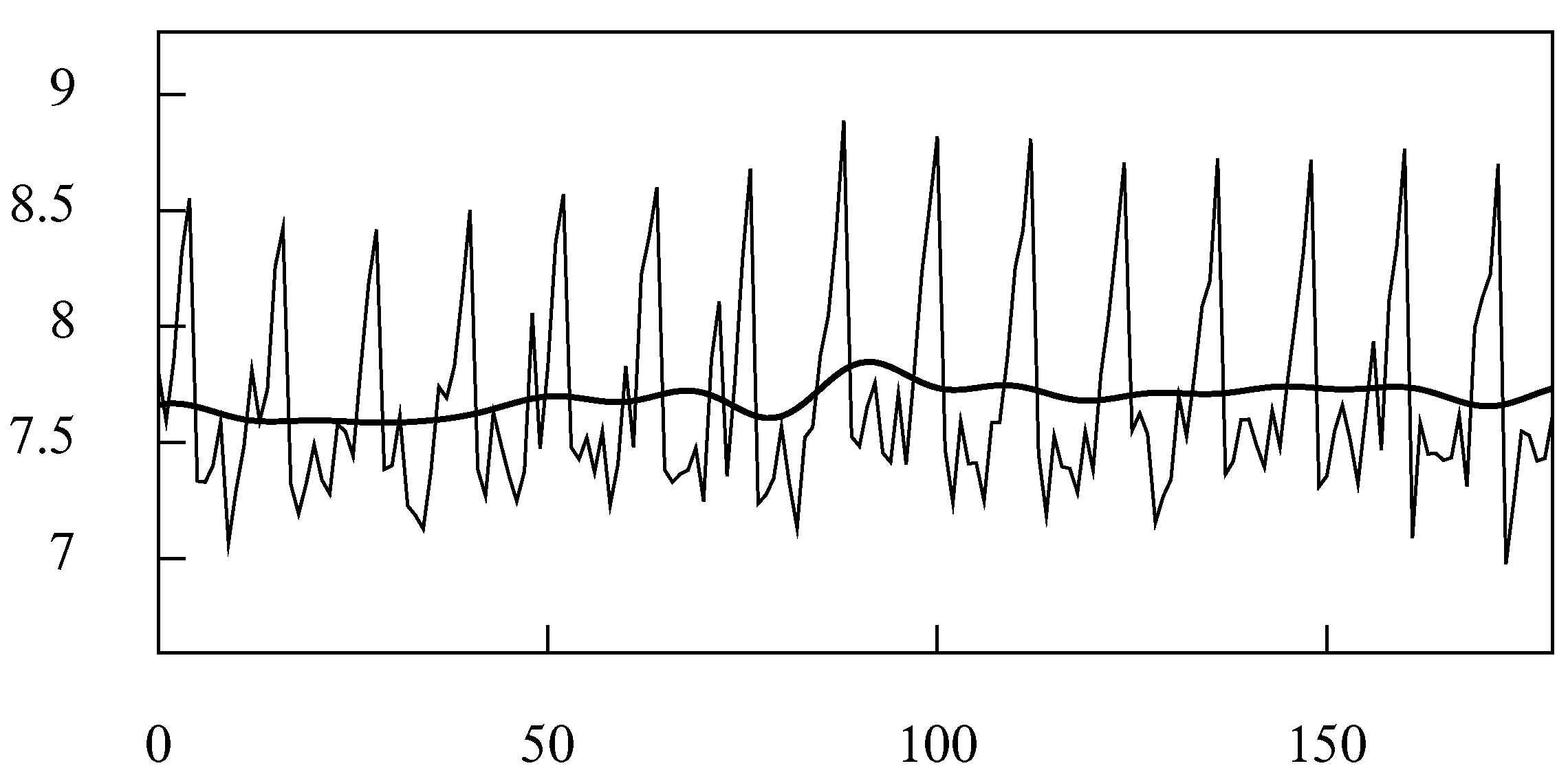
Figure 22 shows the logarithms of 180 values of the monthly sales of sparkling wine in Australia in the period from June 1980 to July 1995. Superimposed on these data is an estimated trend-cycle function that has been extracted by an ideal low pass frequency-domain filter with a cut-off point at ( radians).
The filter has been applied, as the program requires, to the residual deviations of the data from an interpolated polynomial. The polynomial, which is of degree one, corresponds to a straight line. The filtered sequence has been added back to the polynomial to create the trend-cycle function.
Figure 23 shows the periodogram of the residual deviations with the frequency response function of a frequency-domain seasonal adjustment filter superimposed. The seemingly minor elements of the data that fall in the interval correspond to the fluctuations that are added to the polynomial function to create the trend-cycle function.
Surrounding the seasonal frequencies are stop bands of varying widths, described as offsets from those frequencies, which are intended to encompass all of the elements that might be deemed to be contributing to the seasonal fluctuations. The widths are recorded in the following table:
Bordering the stop bands on either side are transition regions of in width, of which the profiles are governed by upper-half cosine functions.
Figure 24 shows the seasonal component that has been extracted from the data. Although this component comprises a significant collection of elements that are adjacent to the seasonal frequencies, it has a surprising regularity.
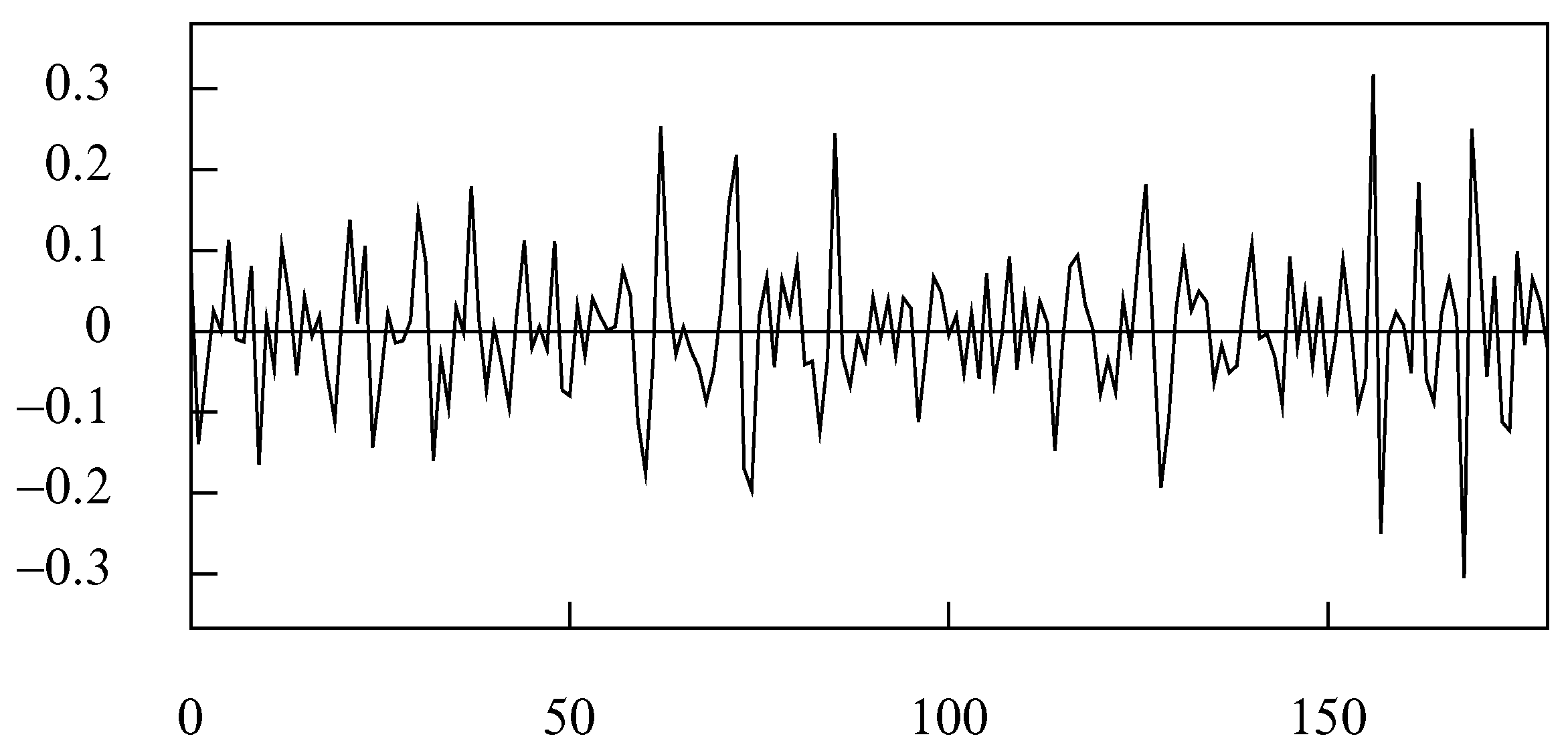
By contrast, the seasonally adjusted data that are shown in Figure 25 have very a rough trajectory. These data may be further decomposed as the sum of the trend-cycle trajectory shown in Figure 22 and a residual noise component that is shown in Figure 26.
Having isolated the residual noise component, one can seek to determine whether it is correlated with any other variables that are within the domain of the economic analysis. If no correlations are discovered and if the outliers cannot be attributed to identifiable economic events, then this component might be disregarded.
Supplementary Materials
The manual for the SEASCAPE program is available online at https://0-www-mdpi-com.brum.beds.ac.uk/2225-1146/9/1/3/s1. The SEASCAPE program and an accompanying collection of data are available at http://www.sigmapi.org.uk/seascape.zip/.
Funding
This research received no external funding.
Data Availability Statement
The data presented in this study accompanies the SEASCAPE program, which is available at http://www.sigmapi.org.uk/seascape.zip/.
Conflicts of Interest
The author declares that there are no conflict of interest.
References
- Attal-Toubert, Ketty, Dominique Ladiray, Marc Marini, and Jean Palate. 2018. Moving Trading-Day Effects with X-13 ARIMA-SEATS and TRAMO-SEATS. In Handbook on Seasonal Adjustment, 2018 ed. Edited by Gian Luigi Mazzi, Dominique Ladiray and Dan A. Rieser. Luxembourg: Eurostat, Publications Office of the European Union, chp. 6. [Google Scholar]
- Box, George E. P., and Gwilym M. Jenkins. 1976. Time Series Analysis: Forecasting and Control, Revised ed. San Francisco: Holden Day. [Google Scholar]
- Caporello, Gianluca, and Agustín Maravall. 2004. Program TSW, Revised Reference Manual. Madrid: Servicio de Estudios, Banco de Espa na. [Google Scholar]
- Findley, David F., Tucker S. McElroy, and Kellie C. Wills. 2005. Modifications of SEATS’ Diagnostic for Detecting over- or Underestimation of Seasonal Adjustment Decomposition Components; Suitland: U.S. Census Bureau.
- Gómez, Victor, and Agustin Maravall. 1997. TRAMO (Time Series Regression with ARIMA Noise, Missing Observations, and Outliers) and SEATS (Signal Extraction in ARIMA Time Series) Instructions for the User. Madrid: Banco de Espana. [Google Scholar]
- Gómez, Victor, and Agustin Maravall. 2001. Seasonal Adjustment and Signal Extraction in Economic Time Series. In A Course in Time Series Analysis. Edited by Daniel Peña, George C. Tiao and Ruey S. Tsay. New York: John Wiley and Sons, chp. 8. [Google Scholar]
- Grudkowska, Sylwia. 2017. JDemetra+ Reference Manual Version 2.2. Available online: https://jdemetradocumentation.github.io/JDemetra-documentation/ (accessed on 1 January 2021).
- Hillmer, Steven Craig, and George C. Tiao. 1982. An ARIMA-Model-Based Approach to Seasonal Adjustment. Journal of the American Statistical Association 77: 63–70. [Google Scholar] [CrossRef]
- Hodrick, Robert J., and Edward C. Prescott. 1997. Postwar U.S. Business Cycles: An Empirical. Investigation. Journal of Money Credit and Banking 29: 1–16. [Google Scholar] [CrossRef]
- Kaiser, Regina, and Agustín Maravall. 2001. Measuring Business Cycles in Economic Time Series. Lecture Notes in Statistics 154. New York: Springer. [Google Scholar]
- Koopman, Siem Jan, Andrew C. Harvey, Jurgen A. Doornik, and Neil Shephard. 1995. STAMP 5.0: Structural Time Series Analyser, Modeller and Predictor. London: Chapman & Hall. [Google Scholar]
- Ladiray, Dominique. 2018. Calendar Effects. In Handbook on Seasonal Adjustment, 2018 ed.; Edited by Gian Luigi Mazzi, Dominique Ladiray and Dan A. Rieser. Luxembourg: Eurostat, Publications Office of the European Union, chp. 5. [Google Scholar]
- Ladiray, Dominique, and Benoit Quenneville. 2001. Seasonal Adjustment with the X-11 Method. Springer Lecture Notes in Statistics 158. Berlin: Springer. [Google Scholar]
- Leser, Conrad Emanuel Victor. 1961. A Simple Method of Trend Construction. Journal of the Royal Statistical Society, Series B 23: 91–107. [Google Scholar] [CrossRef]
- Mazzi, Gian Luig, Dominique Ladiray, and Dan A. Rieser. 2018. Handbook on Seasonal Adjustment, 2018 ed.; Luxembourg: Eurostat, Publications Office of the European Union.
- McElroy, Tucker, and Anindya Roy. 2017. Detection of Seasonality in the Frequency Domain. Journal of Statistical Planning and Inference 221: 241–55, Forthcoming in (2021). [Google Scholar]
- Pollock, D. Stephen G. 2000. Trend Estimation and de-trending via Rational Square Wave Filters. Journal of Econometrics 99: 317–34. [Google Scholar] [CrossRef]
- Pollock, D. Stephen G. 2018. Filters, Waves and Spectra. Econometrics 6: 35. [Google Scholar] [CrossRef] [Green Version]
- Proakis, John G., and Dimitris G. Manolakis. 1996. Digital Signal Processing: Principles, Algorithms, and Applications, 3rd ed. Upper Saddle River: Prentice-Hall. [Google Scholar]
- Shiskin, Julius, Allan H. Young, and John C. Musgrave. 1967. The X-11 Variant of the Census Method II Seasonal Adjustment; Technical Paper No. 15; Suitland: Bureau of the Census, U.S. Department of Commerce.
- Wildi, Marc. 2005. Signal Extraction: Efficient Estimation, Unit Root Tests and Early Detection of Turning Points. Springer Lecture Notes in Economic and Mathematical Systems 547. Berlin: Springer. [Google Scholar]
Figure 1.
The pole-zero diagram of the unidirectional comb filter for monthly data. The poles are marked by crosses and the zeros are marked by circles.
Figure 1.
The pole-zero diagram of the unidirectional comb filter for monthly data. The poles are marked by crosses and the zeros are marked by circles.
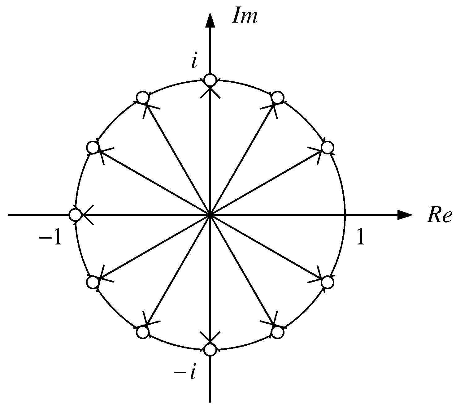
Figure 2.
The frequency response functions of the bidirectional comb filter for monthly data with , giving the lesser peaks, and , giving the higher peaks.
Figure 2.
The frequency response functions of the bidirectional comb filter for monthly data with , giving the lesser peaks, and , giving the higher peaks.
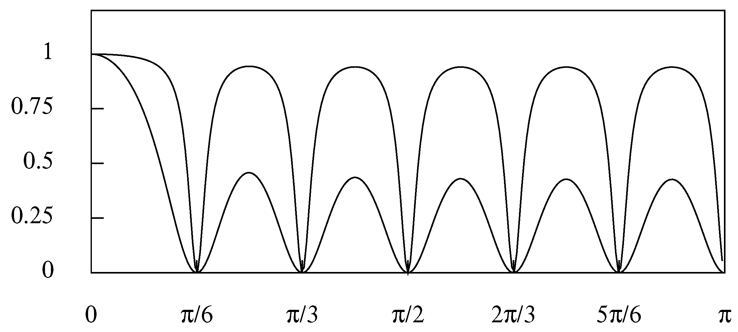
Figure 3.
The frequency response functions of the basic seasonal adjustment filter for monthly data with and (the solid line) and with and (the dashed line).
Figure 3.
The frequency response functions of the basic seasonal adjustment filter for monthly data with and (the solid line) and with and (the dashed line).

Figure 4.
The frequency response function of the basic time-domain seasonal-adjustment filter for quarterly data with . and .
Figure 4.
The frequency response function of the basic time-domain seasonal-adjustment filter for quarterly data with . and .

Figure 5.
The residuals from a linear de-trending of the logarithms of an index of quarterly U.K. consumption for 1955–1994, with a superimposed seasonally-adjusted sequence, derived by the basic time-domain filter.
Figure 5.
The residuals from a linear de-trending of the logarithms of an index of quarterly U.K. consumption for 1955–1994, with a superimposed seasonally-adjusted sequence, derived by the basic time-domain filter.

Figure 6.
The seasonal component extracted by the basic time-domain filter from the logarithms of an index of quarterly U.K. consumption for 1955–1994.
Figure 6.
The seasonal component extracted by the basic time-domain filter from the logarithms of an index of quarterly U.K. consumption for 1955–1994.

Figure 7.
The frequency response function of the double seasonal adjustment filter for monthly data with offsets of two degrees.
Figure 7.
The frequency response function of the double seasonal adjustment filter for monthly data with offsets of two degrees.
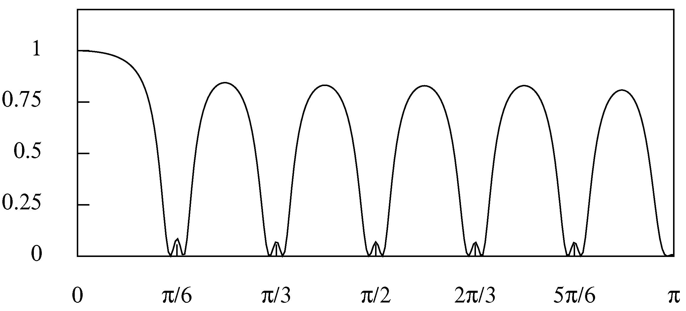
Figure 8.
The frequency response function of the triple seasonal adjustment filter for monthly data with offsets of three degrees.
Figure 8.
The frequency response function of the triple seasonal adjustment filter for monthly data with offsets of three degrees.

Figure 9.
The frequency response of the seasonal-adjustment filter associated with the monthly airline passenger model.
Figure 9.
The frequency response of the seasonal-adjustment filter associated with the monthly airline passenger model.
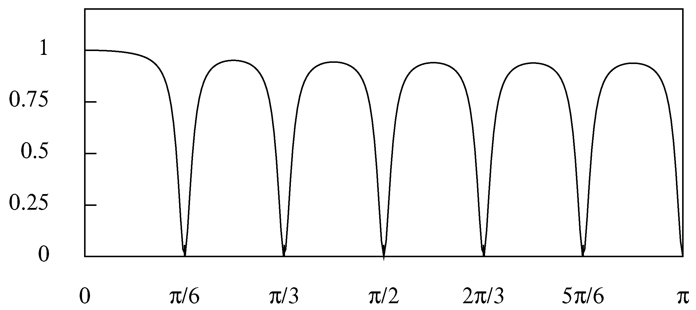
Figure 10.
The frequency response of the trend extraction filter associated with the monthly airline passenger model.
Figure 10.
The frequency response of the trend extraction filter associated with the monthly airline passenger model.

Figure 11.
The frequency response of the composite trend extraction filter that mimics that of the monthly airline passenger model.
Figure 11.
The frequency response of the composite trend extraction filter that mimics that of the monthly airline passenger model.
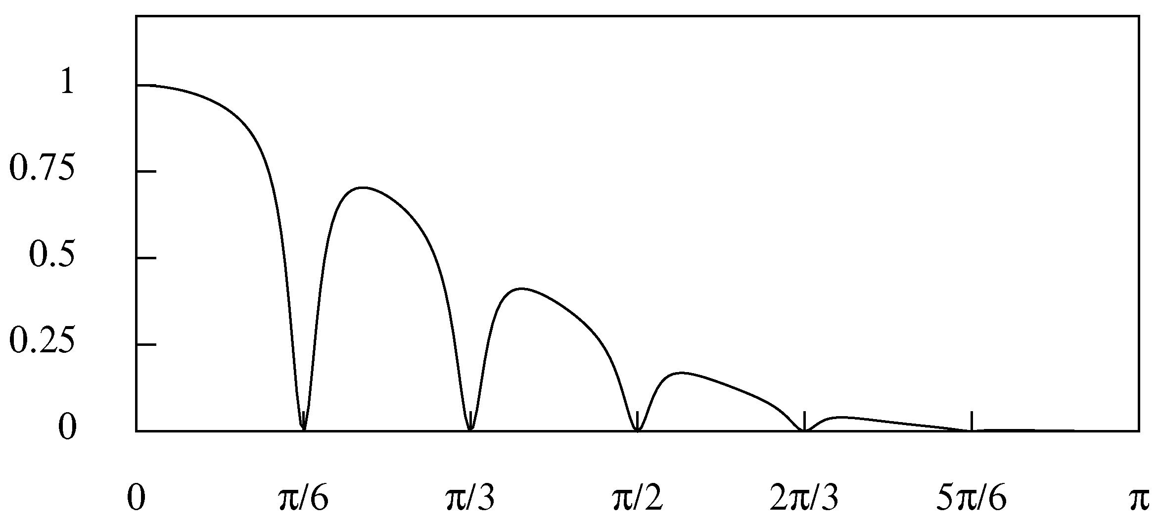
Figure 12.
The effect of applying the trend extraction filter to the sequence depicted in Figure 5.
Figure 12.
The effect of applying the trend extraction filter to the sequence depicted in Figure 5.

Figure 13.
The periodogram of the residual sequence from the linear de-trending of the logarithmic consumption data.
Figure 13.
The periodogram of the residual sequence from the linear de-trending of the logarithmic consumption data.

Figure 14.
The residual sequence from fitting a linear trend to the logarithmic consumption data with an interpolated line representing the business cycle, obtained by the frequency-domain method.
Figure 14.
The residual sequence from fitting a linear trend to the logarithmic consumption data with an interpolated line representing the business cycle, obtained by the frequency-domain method.

Figure 15.
The cosine segments that give rise to: the upper-half cosine transitions (left); and the lower-half cosine transitions (right).
Figure 15.
The cosine segments that give rise to: the upper-half cosine transitions (left); and the lower-half cosine transitions (right).

Figure 16.
The frequency response function of a frequency-domain seasonal adjustment filter for monthly data with stop bands of six degrees in width.
Figure 16.
The frequency response function of a frequency-domain seasonal adjustment filter for monthly data with stop bands of six degrees in width.
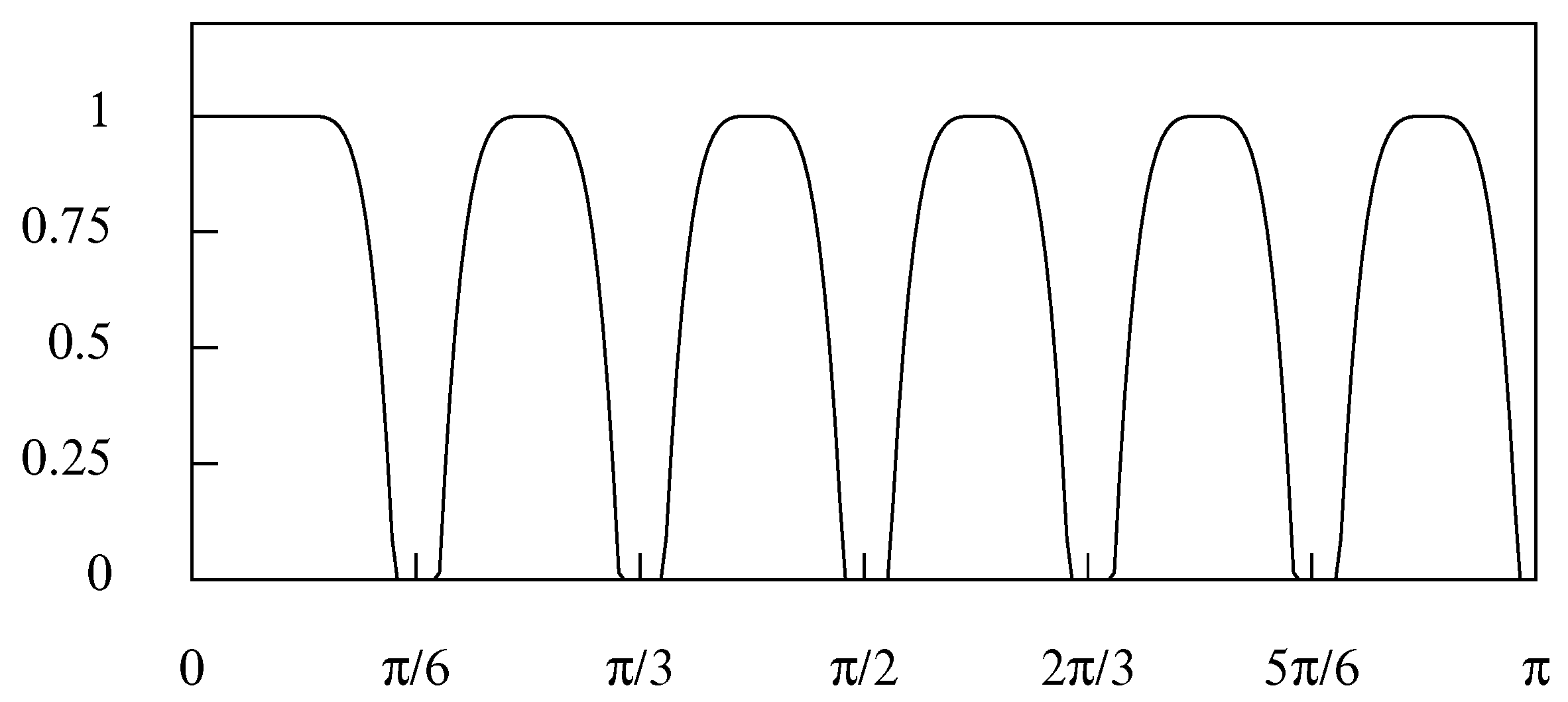
Figure 17.
The frequency response function of a low pass frequency-domain filter with a transition in the interval governed by a composite sigmoid function with , shown by the continuous line. The frequency response of the complementary high pass filter is shown by the dashed line.
Figure 17.
The frequency response function of a low pass frequency-domain filter with a transition in the interval governed by a composite sigmoid function with , shown by the continuous line. The frequency response of the complementary high pass filter is shown by the dashed line.

Figure 18.
The 336 observations of the value in dollars of the monthly sales of women’s clothing is US retail stores, with a superimposed polynomial trend function of degree 4.
Figure 18.
The 336 observations of the value in dollars of the monthly sales of women’s clothing is US retail stores, with a superimposed polynomial trend function of degree 4.

Figure 19.
The periodogram of the data on the sales of clothing with the frequency response of the basic time-domain seasonal adjustment filter superimposed.
Figure 19.
The periodogram of the data on the sales of clothing with the frequency response of the basic time-domain seasonal adjustment filter superimposed.

Figure 20.
The seasonally adjusted data on the sales of clothing.
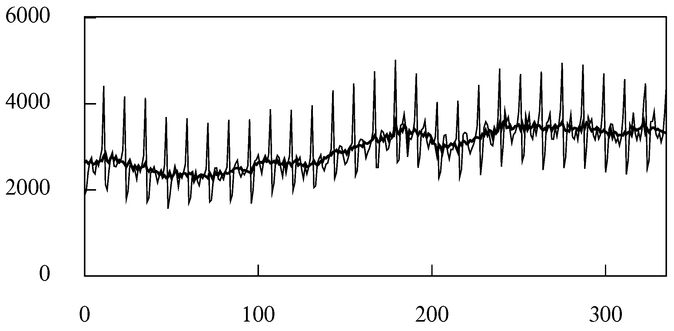
Figure 21.
The trend-cycle function superimposed on the monthly sales of women’s clothing.

Figure 22.
The 187 values of the monthly sales of sparkling wine in Australia in the period from January 1980 to July 1995, with a superimposed trend-cycle function.
Figure 22.
The 187 values of the monthly sales of sparkling wine in Australia in the period from January 1980 to July 1995, with a superimposed trend-cycle function.

Figure 23.
The periodogram of the residuals from a linear de-trending of the wine data, with a superimposed frequency response function of a seasonal-adjustment filter.
Figure 23.
The periodogram of the residuals from a linear de-trending of the wine data, with a superimposed frequency response function of a seasonal-adjustment filter.
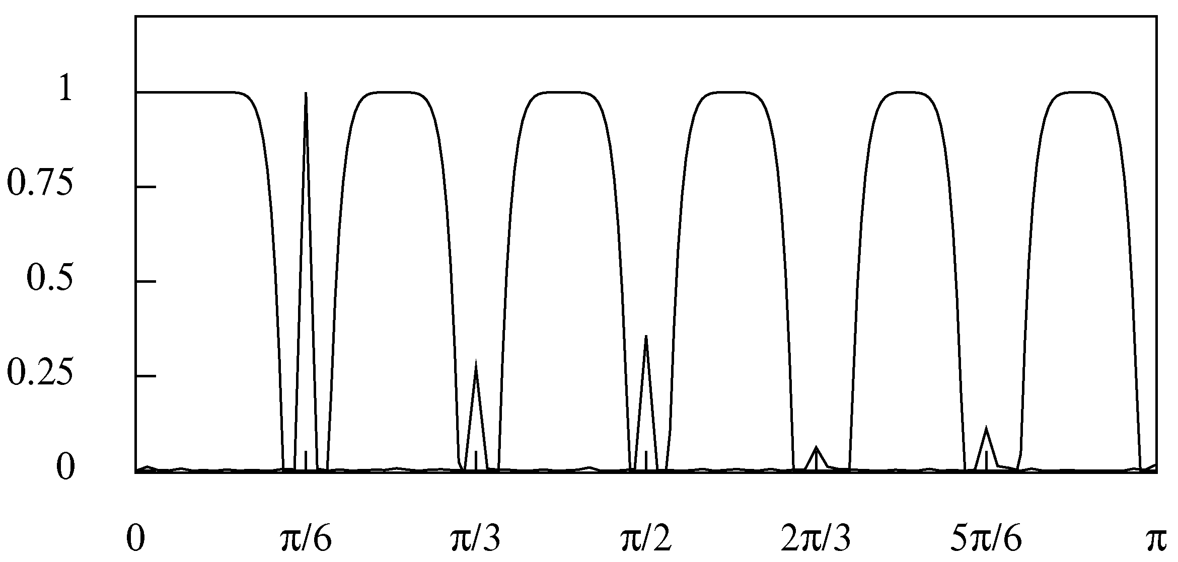
Figure 24.
The seasonal component extracted from the wine data.

Figure 25.
The seasonally adjusted wine data superimposed, as a heavy line, on the original data.

Publisher’s Note: MDPI stays neutral with regard to jurisdictional claims in published maps and institutional affiliations. |
© 2021 by the author. Licensee MDPI, Basel, Switzerland. This article is an open access article distributed under the terms and conditions of the Creative Commons Attribution (CC BY) license (http://creativecommons.org/licenses/by/4.0/).
Share and Cite
MDPI and ACS Style
Pollock, D.S.G. Enhanced Methods of Seasonal Adjustment. Econometrics 2021, 9, 3. https://0-doi-org.brum.beds.ac.uk/10.3390/econometrics9010003
AMA Style
Pollock DSG. Enhanced Methods of Seasonal Adjustment. Econometrics. 2021; 9(1):3. https://0-doi-org.brum.beds.ac.uk/10.3390/econometrics9010003
Chicago/Turabian StylePollock, D. Stephen G. 2021. "Enhanced Methods of Seasonal Adjustment" Econometrics 9, no. 1: 3. https://0-doi-org.brum.beds.ac.uk/10.3390/econometrics9010003
Note that from the first issue of 2016, this journal uses article numbers instead of page numbers. See further details here.