
Temperature Anomalies, Long Memory, and Aggregation


Department of Mathematical Sciences, Aalborg University and CREATES, DK-9220 Aalborg, Denmark
Econometrics 2021, 9(1), 9; https://0-doi-org.brum.beds.ac.uk/10.3390/econometrics9010009
Submission received: 29 October 2020
/
Revised: 18 February 2021
/
Accepted: 24 February 2021
/
Published: 3 March 2021
(This article belongs to the Collection Econometric Analysis of Climate Change)
Abstract
:Econometric studies for global heating have typically used regional or global temperature averages to study its long memory properties. One typical explanation behind the long memory properties of temperature averages is cross-sectional aggregation. Nonetheless, formal analysis regarding the effect that aggregation has on the long memory dynamics of temperature data has been missing. Thus, this paper studies the long memory properties of individual grid temperatures and compares them against the long memory dynamics of global and regional averages. Our results show that the long memory parameters in individual grid observations are smaller than those from regional averages. Global and regional long memory estimates are greatly affected by temperature measurements at the Tropics, where the data is less reliable. Thus, this paper supports the notion that aggregation may be exacerbating the long memory estimated in regional and global temperature data. The results are robust to the bandwidth parameter, limit for station radius of influence, and sampling frequency.
JEL Classification:
Q54; C22; C43; C141. Introduction
From its inception, long memory models have been associated with the analysis of climate data. One of the first works on long memory originates from Hurst (1956). The author studied the long-term capacity of water reservoirs on the Nile. Given the cycles of highs at the river, he recommended increasing the height of a dam to be built. His analysis showed that a dam built based on a short memory model would be more prone to overflow, increasing the risk of a catastrophic event, than one built based on a long memory model. That is, incorporating long memory properties leads to a more accurate characterisation of climate data. Hurst’s observations served as inspiration for Mandelbrot’s work on fractional Brownian motion (see Mandelbrot (1967); Mandelbrot and Van Ness (1968)). The authors labelled this phenomenon the Joseph effect in reference to the “seven years of great abundance” followed by “seven years of famine”.
As recognised by Hurst, assessing the long memory properties of natural phenomena can have major repercussions in policy design. Under the current climate emergency, assessing the long memory properties of temperature data can help to properly evaluate the pace of global heating and its likely repercussions.
In a recent analysis, Calel et al. (2020) show that uncertainty plays a major role in computing the economic costs of climate change. The authors show that studies that do not incorporate all uncertainties can vastly underestimate the economic costs. Furthermore, they argue that long memory properties in temperature data can result in estimates of even greater economic damages thus, they appeal for a proper characterisation of the long-term temperature dynamics.
It has been shown that failing to account for long memory dynamics can result in spurious regressions (see Marmol (1995), Tsay and Chung (2000), and Ventosa-Santaulària et al. (2020)). Linear models to explain global heating could provide misleading results if they do not control for the long memory in the data. Thus, assessing the long memory properties of temperature data is of major theoretical and applied relevance.
Bloomfield (1992) and Bloomfield and Nychka (1992) are among the first to use long memory models in the analysis of temperature data. The authors noted that long memory should be incorporated in trend estimations for temperature series to obtain correct confidence intervals. More recently, Baillie and Chung (2002) and Mills (2007) use fractionally differenced models to estimate the long memory parameter, while Gil-Alana (2005) and Mangat and Reschenhofer (2020) use semiparametric estimators in the frequency domain. They all conclude that temperature data possess long memory. Nonetheless, they differ as to the degree of memory. The distinction is relevant given that a large degree of memory implies a nonstationary process or even a process that does not revert to the mean.
Most articles have focused on analysing regional or global average temperature anomalies. In this regard, several authors have argued that aggregation may be the reason behind the presence of long memory in the data (see Baillie and Chung (2002); Gil-Alana (2005); Mills (2007)). Nonetheless, to the best of our knowledge, there is no formal analysis of whether aggregation may explain long memory in temperature data. Thus, this paper looks to determine the role aggregation has on the presence of long memory in temperature data. The analysis relies on estimating the long memory parameters in the individual grid temperature series and comparing them against regional and global averages.
We use data from the Goddard Institute for Space Studies Surface Temperature Analysis (GISTEMP) and estimate the long memory parameters using semiparametric estimators in the frequency domain. The data is further detailed in Section 2, while the long memory estimators are presented in Section 3. Our results, presented in Section 4, show that the long memory parameters in individual grid observations are lower than for the regional averages. The long memory dynamics for the aggregated data seems to be greatly affected by measurements around the Tropics, where data is less reliable. Thus, our results support the notion that aggregation may be exacerbating the long memory estimated in aggregated temperature data.
2. Temperature Anomalies
The GISTEMP data is an estimate of global surface temperature change constructed by the NASA Goddard Institute for Space Studies (GISS). GISS specifies the temperature anomaly at a given location as the weighted average of the anomalies for all stations located in close proximity. A total of 16,200 grid observations are reported, along with several regional temperature averages. The data is updated monthly and combines data from land and ocean surface temperatures (see GISTEMP Team (2020); Lenssen et al. (2019)). GISTEMP is publicly available at data.giss.nasa.gov/gistemp/ (accessed on 18 February 2021).
It is important to point out that our analysis does not impute any missing data. Instead, we focus on the most recent subsample without missing observations for each grid. We discard grids with less than 50 observations in the last subsample without missing observations. A total of 219 grids out of 16,200 are removed from the analysis. The design allows us to have a large enough sample size for long memory estimation without introducing imputation uncertainties.
Figure 1 shows the temperature anomalies for August 2020 against the 1951–1980 baseline. The figure shows the temperature anomalies at individual grids across the globe considering a 1200 km smoothing radius; that is, each grid considers stations located within 1200 km from the specified grid point. A similar map can be plotted for each month since 1850. Additionally, GISTEMP presents data using a 250 km smoothing radius, which we will use in our analysis as part of our robustness exercises.
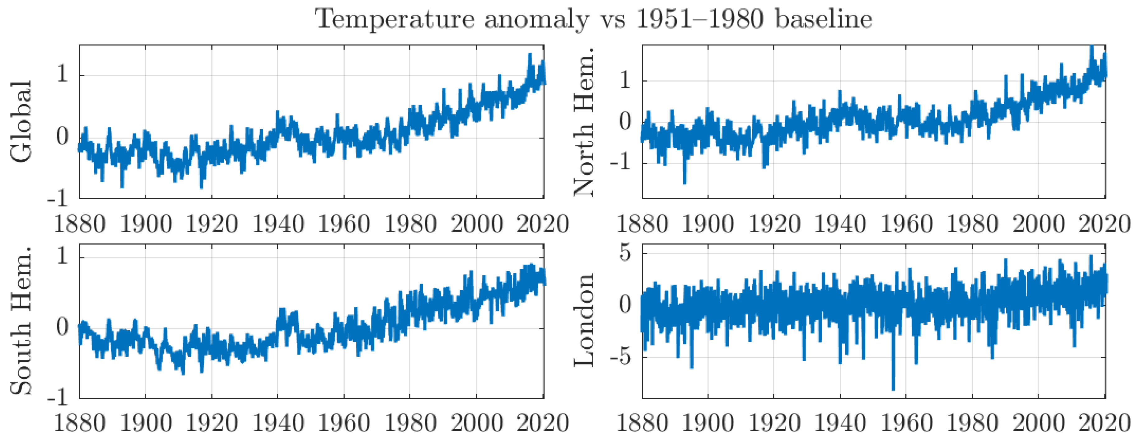
Given the vast amount of information contained in GISTEMP, regional and global temperature averages are typically considered in climate econometrics research. Figure 2 shows global, Northern Hemisphere, and Southern Hemisphere temperature anomalies data reported by GISTEMP. Our goal is to compare the dynamics of these regional aggregates against individual grid data.
It would be unwieldy to plot the time series data for all individual grids. Hence, we have selected a representative candidate for the individual grid observations. For illustrative purposes, the figure shows the temperature anomaly series for the grid containing London, (,). We select the London grid given that it contains a large city and thus reliable measurements are available.
This paper argues that the long memory properties of the regional and global series are affected by cross-sectional aggregation. To test this hypothesis, we estimate the long memory parameters for the temperature data at all grids shown in Figure 1 and compare them against the long memory estimates for the regional temperature data shown in Figure 2.
3. Methods
3.1. Long Memory
The study of long memory in econometrics goes back to Granger’s (1966) research on the shape of the spectrum of economic series. Granger found that the spectrum diverges to infinity as the frequency goes to zero for many financial and economic series, what the author called “the typical shape”. This kind of behaviour has led to several definitions of long memory. This paper considers three of the most common definitions of long memory, which are presented in the following definition.
Definition 1.
Let be a time series with autocovariance function , and spectral density function , and let , then has long memory:
- (i).
- In the spectral sense if as with a constant;
- (ii).
- In the self-similar sense if as where , with , , and is a constant;
- (iii).
- In the covariance sense if as with a constant.
Above, is the covariance function between x and y, as means that converges to 1 as x tends to , and d is called the long memory parameter. Furthermore, the process is shown to be stationary if , and it reverts to its mean if .
Definition 1(i) is the feature discussed by Granger (1966) in his study of the typical spectral shape of economic variables. The definition is based on the property that the spectral density for a long memory process has a pole at the origin. The behaviour of the spectrum near the origin is also used in the construction of semi-parametric estimators in the frequency domain (see Section 3.3).
Definition 1(ii) is based on the work on fractals and self-similarity by Mandelbrot and Van Ness (1968). Self-similarity implies that the degree of memory is asymptotically equivalent for different levels of temporal aggregation. Thus, asymptotically, the long memory parameter is statistically the same whether we estimate it at different sampling frequencies. This property is relevant for the study of temperature data given that the literature has used both monthly and yearly data to test for long memory properties. Under self-similarity, the long memory parameter estimates are statistically equivalent in both sampling frequencies. However, the shortened sample size must be considered when estimating the long memory parameter on yearly data.
Definition 1(iii) is concerned with the behaviour of the autocorrelation function for large lags. It was one of the motivations behind the AutoRegressive Fractionally Integrated Moving Average (ARFIMA) class of models due to Granger and Joyeux (1980) and Hosking (1981). They proposed to use the fractional difference operator to induce slowly decaying autocorrelations.
Figure 3 shows the autocorrelation functions for global, Northern Hemisphere, and Southern Hemisphere temperature anomalies data. The autocorrelation functions exhibit hyperbolic decay. In particular, they are above one half even after a hundred lags. That is, temperature data exhibits long memory in the covariance sense.
For illustrative purposes, the figure also shows the autocorrelation function for the grid containing London. The regional and global averages decay at a slower pace than the individual temperature grid, suggesting a smaller degree of memory for the individual grid data. The shaded area covers from the first to third quartile of the autocorrelation functions for all individual grids. Thus, the figure shows that the the behaviour of the autocorrelation function at the London grid resembles the typical shape for the autocorrelation functions at other grids. Moreover, Figure A1 in Appendix A presents boxplots for the autocorrelation functions at all grids. The figure further shows that the dynamics at the grid near London are similar to the dynamics at most grids.
3.2. Cross-Sectional Aggregation
Long memory by cross-sectional aggregation was first discussed by Granger (1980). The author showed that long memory can result from aggregation fof short memory processes. He considered the process defined by:
where , and each is an independent autoregressive process with random coefficient given by:
where is an independent identically distributed process with , and , . Furthermore, is sampled from the Beta distribution, independent from .
Granger (1980) showed that taking a large number in the cross-sectional dimension the resulting process will exhibit long memory in the covariance sense, see Definition 1(iii). Haldrup and Vera-Valdés (2017) extended Granger’s result to show that cross-sectionally aggregated processes possess long memory according to all definitions considered in Definition 1.
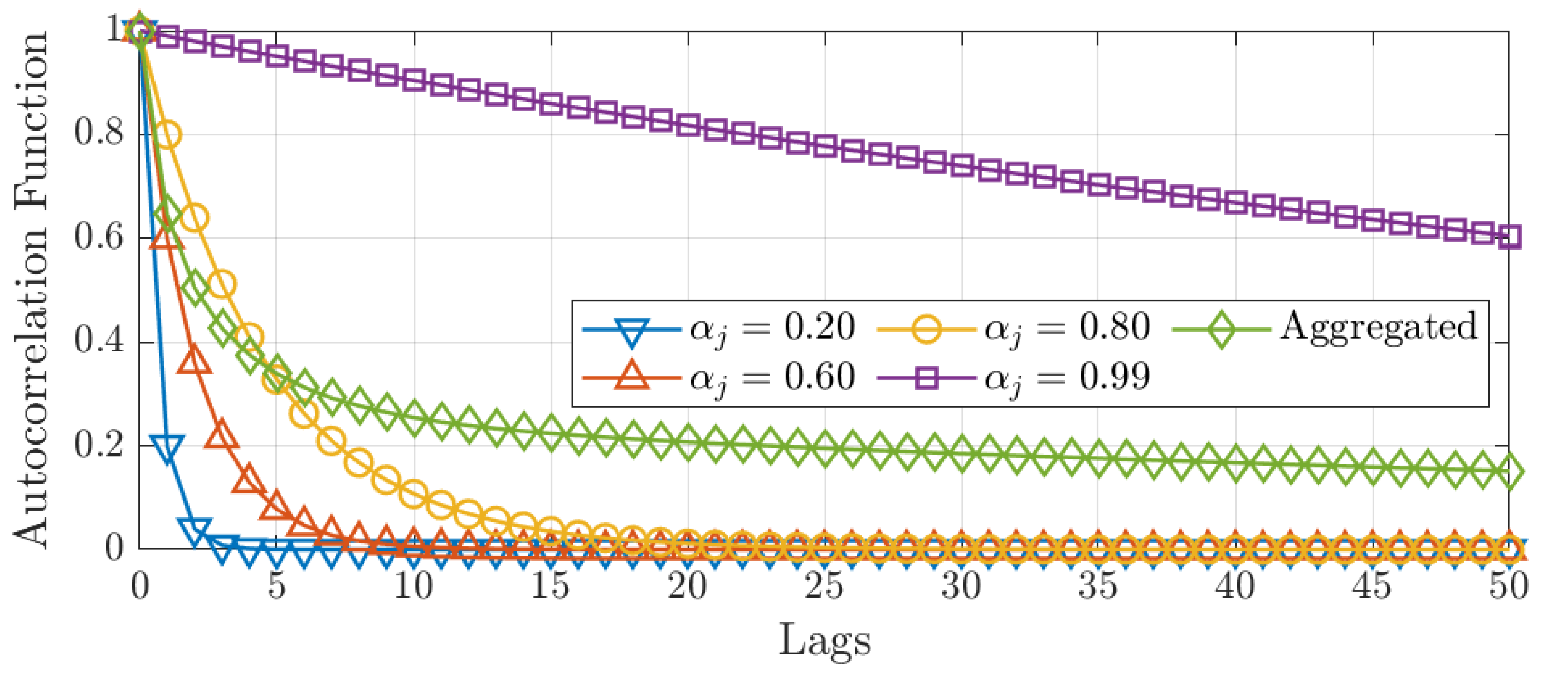
The aggregation argument is illustrated in Figure 4.
The figure shows the autocorrelation functions for four autoregressive processes with different autoregressive parameter, and the autocorrelation function for the aggregated process, Equation (1). As can be seen, the autocorrelation function of the aggregated process exhibits hyperbolic decay consistent with long memory in the covariance sense. In this regard, the aggregation argument proves that the degree of memory of the aggregated series is non-zero. Meanwhile, the degrees of memory of the four autoregressive processes are zero by construction. Thus, the aggregated series has a larger degree of memory than the average of the degrees of memory of the four individual series.
As argued by Granger (1980), the degree of memory of the aggregated process is determined by the autoregressive process’ probability mass around one. The more likely it is to obtain near-unit root processes in the aggregate, the greater the degree of memory. An example of this argument can be seen in Figure 4. The long-term behaviour of the aggregated process is influenced by combining three autoregressive processes with a coefficient away from one with one autoregressive process with a near-unity coefficient. Intuitively, the near-unity process pulls on the autocorrelation function of the aggregate. In this regard, the more autoregressive processes with coefficients near unity, the greater the degree of memory in the aggregate.
The cross-sectional aggregation result has been extended in several directions, including to allow for general AutoRegressive Moving Average (ARMA) processes, as well as to other distributions, see Linden (1999), Oppenheim and Viano (2004), and Zaffaroni (2004), to name a few. Furthermore, Vera-Valdés (2020) has shown that the fractional difference operator produces well-performing forecasts for aggregated processes via simulations.
In economic data, cross-sectional aggregation plays a significant role in long memory generation. Cross-sectional aggregation has been cited as the source of long memory for inflation, output, and volatility; see Balcilar (2004), Diebold and Rudebusch (1989), Altissimo et al. (2009), and Osterrieder et al. (2019). As pointed in Section 1, aggregation has been cited as the explanation behind the presence of long memory in temperature data given its reliance on temperature aggregates.
One important distinction regarding long memory generated by aggregation is that it does not belong to the class of processes generated using the fractional difference operator (see Haldrup and Vera-Valdés (2017)). In particular, the autocorrelation function for the aggregated process does not correspond to the autocorrelation function of any ARFIMA process. Thus, parametric estimators based on the fractional difference operator are misspecified for long memory processes by cross-sectional aggregation. Nonetheless, given that aggregated processes are long memory in the spectral sense, we can consistently estimate the long memory parameter in the frequency domain.
3.3. Semiparametric Estimators of Long Memory
The semiparametric estimators in the frequency domain are based on the long memory definition in the spectral sense, see Definition 1(i). The idea is to evaluate the periodogram of the time series, an estimator of the spectral density, in a vicinity of the origin where the long memory parameter drives the spectral density. Focusing on the vicinity of the origin further circumvents the need to specify the short-term dynamics of the data. Indeed, the semiparametric estimators are robust to short-run dynamics like observational noise.
Long memory estimators in the frequency domain are typically divided between the log-periodogram regression method proposed by Geweke and Porter-Hudak (1983), and the local Whittle approach developed by Künsch (1987).
On the one hand, the log-periodogram regression (GPH, from now on) is given by:
where is the periodogram of , are the Fourier frequencies, c is a constant, is the error term, and m is a bandwidth parameter that grows with the sample size. The zero frequency is not included in (3), making the estimator robust to the specification of the mean.
The consistency and asymptotic normality of the log-periodogram regression have been proved by Robinson (1995b); Velasco (1999b, 2000). Denote to the estimate of the long memory parameter via the log-periodogram regression, the authors show that:
where m is the bandwidth as before, and denotes convergence in distribution.
Andrews and Guggenberger (2003) (AG, from now on) proposed to replace the constant in (3) with a polynomial in to reduce the bias. The polynomial only considers even degrees given that odd degrees do not help in reducing the bias. In classical bias-variance trade-off, the reduction in bias comes at the cost of an increase in the variance, which depends on the degree of the polynomial used for estimation. For our analysis, we add one polynomial term in (3), which results in the variance of the estimate of 2.25 times the one shown in (4).
On the other hand, Künsch (1987) used a likelihood approach in the so-called local Whittle estimator (LW, from now on). The author proposed to estimate the parameter as the minimiser of the local Whittle likelihood function given by:
where is the periodogram of , are the Fourier frequencies, and m is the bandwidth parameter.
The consistency and asymptotic normality of the local Whittle estimator have been proved for regions of d that are empirically relevant in most application by Phillips and Shimotsu (2004); Robinson (1995a); Velasco (1999a). Denote to the estimate of the long memory parameter via the local Whittle estimator, the authors show that:
where m is the bandwidth as before. In particular, the local Whittle estimator has less variance than both estimators by log-periodogram regression above.
A further refinement to the local Whittle approach was suggested by Shimotsu and Phillips (2005). The authors proposed the exact local Whittle estimator as the minimiser of the function given by:
where is the periodogram of , where is the fractional difference operator, are the Fourier frequencies, and m is the bandwidth parameter.
The exact local Whittle estimator was later extended to allow for nonzero means and time trends in the so-called feasible exact local Whittle (FELW, from now on); see Shimotsu (2010). Furthermore, the author shows that the consistency and asymptotic normality of the FELW are the same as for the local Whittle estimator.
Our preferred method uses the mean-squared error optimal bandwidth of , where T is the sample size, for all the estimators. The optimal bandwidth was obtained by Hurvich et al. (1998). Nonetheless, we consider the commonly used bandwidth of to allow for easy comparisons of other research, and as a robustness exercise.
The variances of the semiparametric estimators of long memory only depend on the bandwidth, which directly depends on the sample size (see (4) and (6)). Thus, estimates using the same bandwidth and approximately the same sample size will exhibit similar uncertainty. Our analysis will use this property to discuss statistical significance while avoiding duplicating standard errors multiple times. Nevertheless, the analysis using yearly observations may suffer from increased uncertainty in the estimates given the reduced sample size. However, following the self-similar property of long memory processes, they are asymptotically equivalent, see Definition 1(ii).
4. Results
This section shows the results from estimating the long memory parameter using semiparametric estimators in temperature anomalies data. We consider temperature anomalies in individual grids and compare them against regional and global averages. Our preferred method uses the optimal bandwidth and the larger monthly datasets. As a robustness exercise, yearly data, different smoothing radius, and values for the bandwidth parameter are considered.
4.1. Monthly Data with 1200 km Smoothing Radius and Optimal Bandwidth
Table 1 presents the long memory estimates from the monthly regional and global temperature averages computed by GISS; that is, the data presented in Figure 2. The table also presents the standard deviation for all estimates. Recall that the standard deviations of the semiparametric long memory estimators depend only on the bandwidth and sample size. Given that all series considered in the table have the same sample size, the standard deviations are the same for all estimates.
The long memory estimates for the regional and global averages imply that they follow a nonstationary process, . Nevertheless, all long memory estimates imply processes that revert to the mean, . We will compare these values against the long memory estimates at all individual grids.
For illustrative purposes, the table shows the long memory estimates for the London grid series. The long memory parameters are statistically larger for the regional and global averages than for the London grid. In particular, all estimates from the regional and global averages are more than four standard deviations apart from the individual grid estimates. That is, the confidence intervals do not intersect, and are thus statistically different.
As previously discussed, GISTEMP contains individual temperature data for 16,200 grids. It will be unwieldy to present a table with long memory estimates for the temperature at all grids. Instead, Figure 5 presents the results for all individual grid points in a global map for each estimator considered.
The figure presents some interesting findings.
First, the degree of memory is smaller for land than for ocean surface temperature. This could relate to the ocean’s larger ‘thermal inertia’ (see Hansen et al. (2010); Sutton et al. (2007)). The authors analyse the common finding that temperatures over land increase more rapidly than over the sea. In this regard, the larger thermal inertia manifests itself in larger degrees of memory.
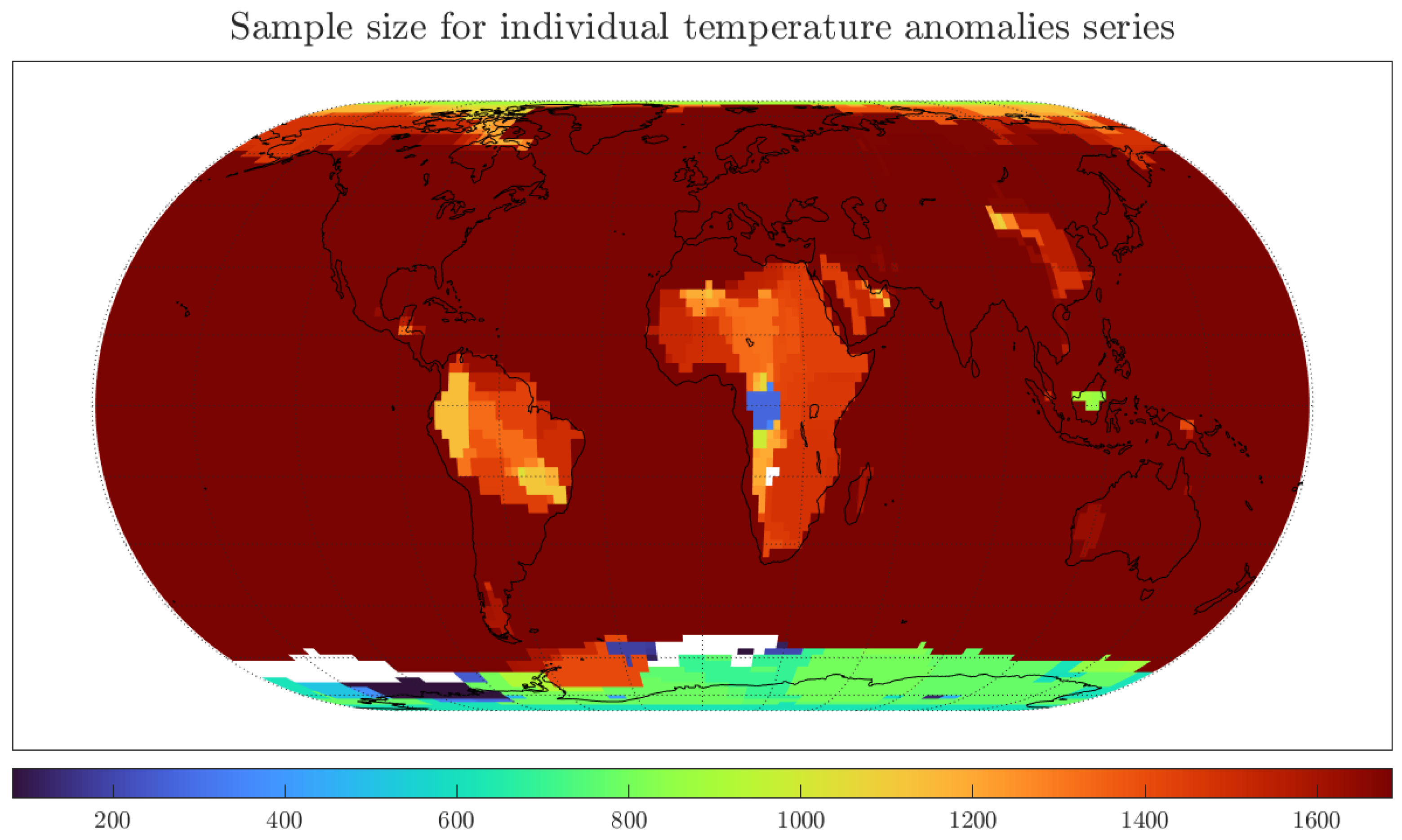
Second, long memory estimates at individual land grids seem to be in the stationary range, , particularly for grids besides Africa and South America. Thus, the degrees of memory near all individual land temperature grids are smaller than those for regional and global averages. The larger degree of memory for temperatures around Africa and South America could relate to increased uncertainty due to the smaller number of long temperature measuring stations in these regions, see Peterson and Vose (1997), and Figure A2 in Appendix A.
Third, besides a few ocean grid temperatures using the LW and FELW estimators, all long memory estimates are in the mean-reverting range, . This indicates that shocks to the temperature series seem to be non-permanent. This result has major implications in terms of the discussion regarding ways to mitigate climate heating. If the degree of memory of temperature data is in the mean-reverting range, we would expect the increase in temperature to revert in the long-run, provided that we implement climate heating mitigating policies.
Finally, the degree of memory of the London grid is in the same range as most of the land temperature grids away from the Equator. Moreover, the sample size for the London grid is comparable to the sample sizes for most of the individual grid series, see Figure A2 in Appendix A. Thus, the standard deviations for all estimates, reported in Figure A3 in Appendix A, are similar to those shown in Table 1. In turn, the discussion regarding the statistical difference between long memory estimates at individual grid temperatures and long memory estimates for regional and global averages extends to most grid series. As previously argued, the London grid shows behaviour similar to other individual grids and its selection is done for illustrative purposes. The figures show that the results extend to most of the land temperature grids.
Overall, the results from Figure 5 suggest that the long memory dynamics for the global and regional averages are greatly affected by aggregation, particularly due to the influence of temperatures at the Tropics. The estimates from the less reliable temperature measurements at Africa and South America, mixed with the higher degrees of memory of temperature at the oceans, propagate due to aggregation to the global and regional long memory estimates.
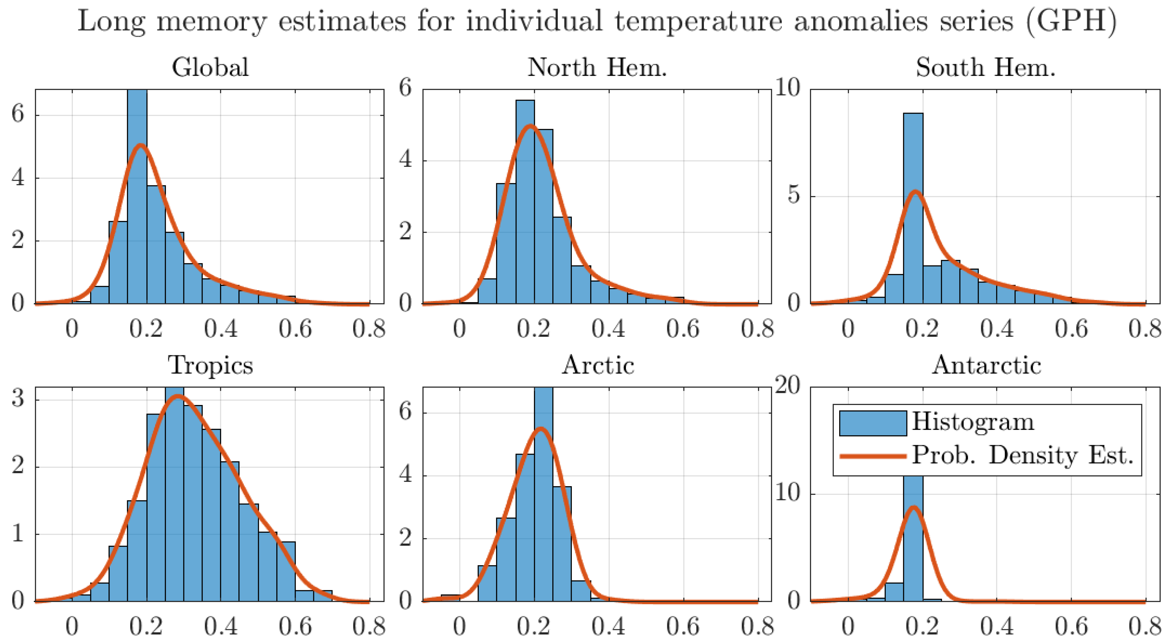
To shed light on the influence that aggregation and the temperature data at the Tropics has on the long memory estimates, Table 2 presents averages from the long memory estimates in individual grid stations for selected regional subsamples. The table shows mean values for the long memory estimates for all grids, the global estimate as well as for grids in the Northern and Southern Hemispheres. Furthermore, the table shows long memory estimate averages for grids located in the Tropics, the Arctic, and Antarctic, that is, those between latitudes and , and , and and , respectively.
Table 2 presents some interesting findings.
First, the averages of the degrees of memory for global and regional temperature grids are smaller than the degrees of memory estimated for the aggregated data. In particular, the global average of the degrees of memory is almost half that of the degree of memory of the global temperature series. The smaller average degrees of memory can be explained due to the smaller degrees of memory estimated for most temperature grids, as shown in Figure 5. This is in line with the aggregation argument explained in Section 3.2, and it provides evidence that aggregation seems to be exacerbating the estimated degrees of memory for global and regional temperature series.
Second, the table broadly confirms that the degree of memory seems to be smaller as we move away from the Tropics. Only the average degree of memory at the Tropics seems to fall into the nonstationary range, and only for the LW and FELW estimators. Thus, the table suggests that the temperature at a few grids around the Tropics increases the degree of memory for the global and regional temperature averages.
Finally, the last column of Table 2 shows the number of individual grids used to compute the regional averages. Note that each region’s number of grids is consistent with equally spaced grid points and a total number of grids of 15,981 once we remove the 219 with no more than 50 observations. That is, around 8000 grids for each hemisphere, or half the total, which is more than 5000 grids for the Tropics, covering a third of the world, and more than 2000 for the Arctic and Antarctic that cover approximately an eight of the globe.
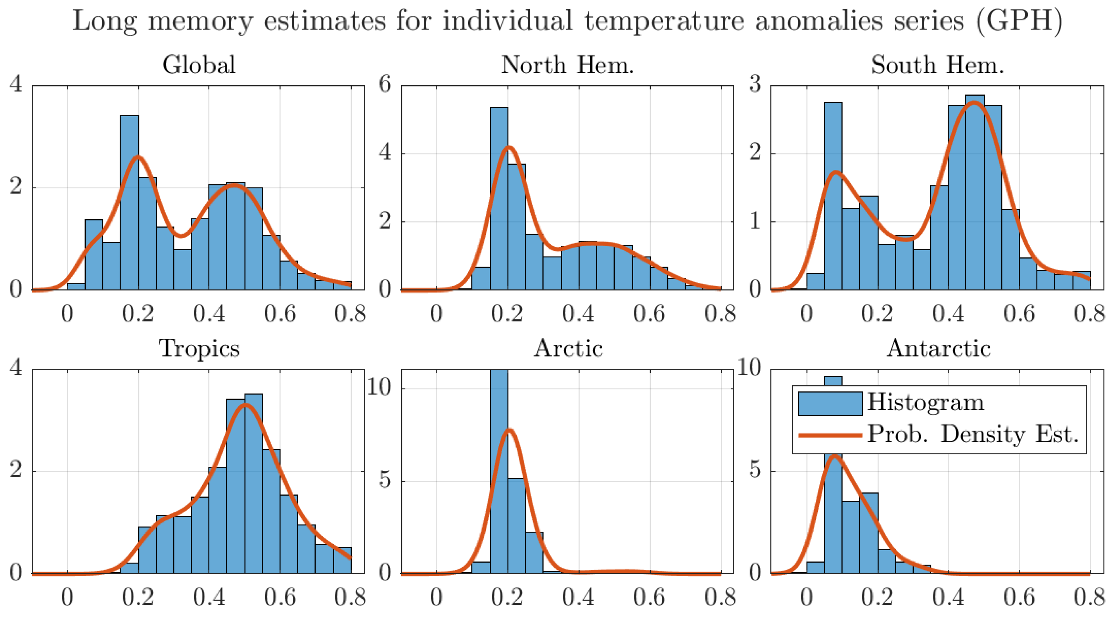
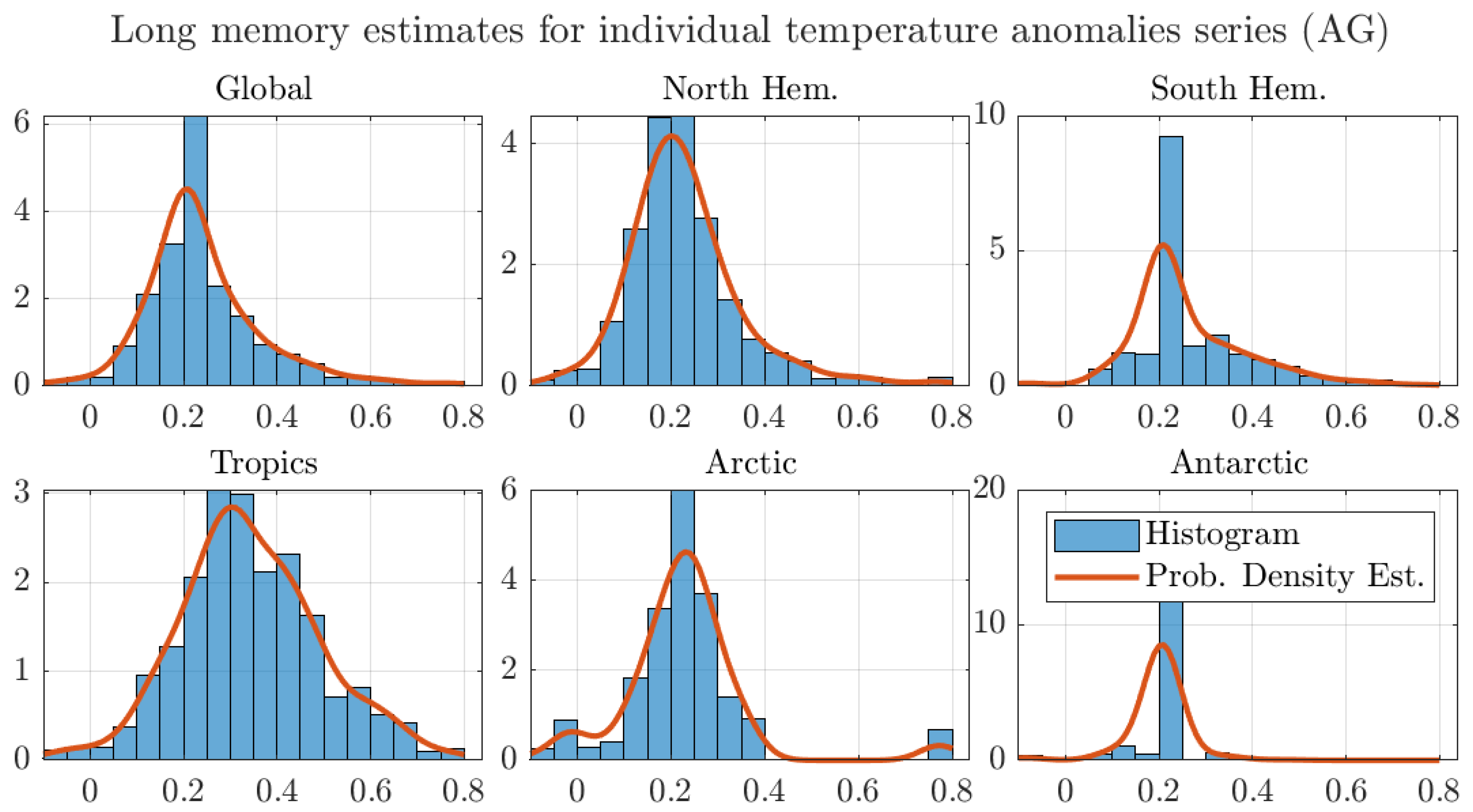
The effect that the memory estimates around the Tropics have on the regional aggregates is further illustrated in Figure 6. The figure shows histograms and estimated probability densities for the long memory estimates for all regions considered in Table 2. For ease of exposition, the figure shows the estimates by the AG method and similar figures for the other estimators are reported in Appendix A.
The figure shows that the probability density of the estimates around the Tropics puts more weight in the nonstationary range than the densities for the other regions. Using an analogous argument to the one in Figure 4, this larger weight to nonstationary values results in a larger degree of memory for the regional average. The same effect can be observed in all regions. In particular, both the Arctic and Antarctic regional estimates assign almost no weight to the nonstationary region, which results in degrees of memory well inside the stationary range. Finally, the figure shows that the mean values are in the stationary range, as shown in Table 2. As previously discussed, the aggregation argument explains the larger degree of memory of the aggregated series in comparison to the average of the degrees of memory of the individual grid series.
4.2. Monthly Data with 250 km Smoothing Radius and Optimal Bandwidth
Figure 7 presents the results for all individual grid points for the 250 km smoothing radius dataset and optimal bandwidth.
The figure shows that the long memory estimates are smaller for the smaller smoothing radius. In particular, almost all long memory estimates are in the stationary range. This once again points to the effect that aggregation has on the long memory estimates. The smaller smoothing radius corresponds to fewer temperature measurements in the averages, translating to smaller degrees of memory due to aggregation.
A thorough analysis of the long memory estimates and standard deviations, reported in Figure A4 in Appendix A, shows that the London grid results are not exceptional and are replicated for most land grids. In particular, the statistical analysis for the London grid extends to other grids.
The figure shows that there is information for fewer grids at the smaller smoothing radius, particularly at sea and around the Tropics. As previously discussed, these missing observations result from the fewer long temperature measuring stations in these regions (see Peterson and Vose (1997)). In turn, the smaller number of temperature grids translates into smaller degrees of memory for the regional averages, as shown in Table 3.
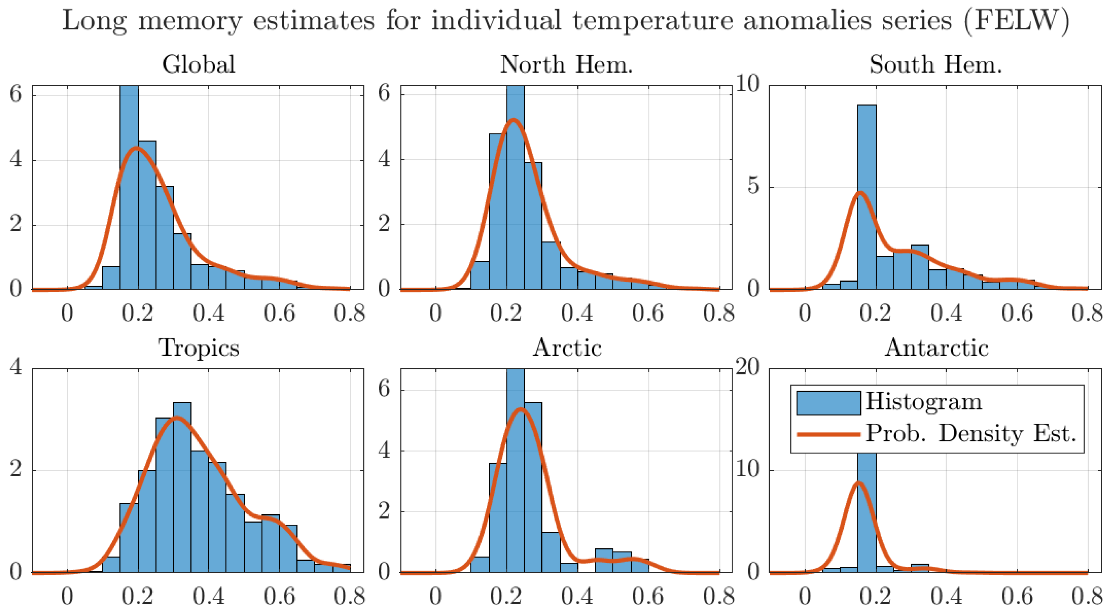
To illustrate the effect that aggregation has on the regional averages, Figure 8 shows the long memory histograms and probability density estimates. For ease of exposition, the figure shows the estimates by the GPH method. Similar figures for the other estimators are reported in Appendix A.
The figure shows that long memory estimates for regions away from the Tropics put no weight to the nonstationary range. Following the aggregation argument, the smaller weight translates into smaller degrees of memory for all regional averages, particularly for the Arctic and Antarctic.
Overall, the results from the smaller smoothing radius agree with the results of our preferred method. Aggregation seems to exacerbate the long memory estimates of global and regional temperature averages. The smaller cross-sectional dimension associated to a reduced smoothing radius results in smaller degrees of memory for the individual temperature grids.
4.3. Robustness Exercises
This section presents the results from some of the robustness exercises considered in this study. In particular, Table 4 and Table 5 show results using yearly data for the 250 km smoothing radius dataset. Table 4 presents the results using the optimal bandwidth, while Table 5 uses the commonly used bandwidth given by , where T is the sample size.
The results from the robustness exercise broadly agree with the main results of this paper. That is, the degrees of memory of an individual grid series is smaller than for the aggregated series, and the degree of memory decreases as we move away from the Tropics. Nonetheless, the reduced sample size product of considering yearly observations increases the variance of all estimates, making them less reliable. Recall that the standard errors for the semiparametric estimators of long memory only depend on the bandwidth parameter and sample size. Thus, smaller sample sizes imply larger standard errors.
Decreasing the bandwidth also increases the variance of the estimates. Hence, the degrees of memory estimated in Table 5 are even more uncertain than those presented in Table 4. However, as argued before, they point to the same conclusions as those from the larger dataset.
Finally, note that the results from Table 5 are in line with the ones from Mangat and Reschenhofer (2020). The authors use some of the semiparametric estimators considered in this study along with the small-sample estimator developed by Reschenhofer and Mangat (2020). Using the same sampling frequency and bandwidth, the authors found that global and regional temperature series fall into the nonstationary range. Furthermore, the authors found some of the long memory estimates for regional temperature series to imply processes that do not revert to the mean, . Our analysis suggest that these results may come from a small bandwidth and sample size.
Additional robustness exercises considering all combinations of the sampling frequency, smoothing radius, and bandwidth all point broadly in the same direction, and they are available upon request.
5. Discussion
The current climate emergency makes it crucial to characterise the long term dynamics of temperature data. In the econometric literature, most climate studies have focused on analysing regional or global average temperature data given the vast amount of information in temperature data. Using regional temperature data, the literature has shown that temperature anomalies possess long memory properties. While several authors have pointed to aggregation as a possible explanation behind the long memory in temperature data, to the best of our knowledge, no analysis has focused on determining if aggregation can indeed be the long memory generating mechanism for temperature data.
This paper looked to determine if aggregation is behind the presence of long memory in global and regional temperature data. The analysis relied on estimating the long memory parameters in individual grid temperature series and comparing them against the regional and global averages. We considered several regional averages in addition to the ones commonly used in the literature. The long memory parameters were obtained using semiparametric estimators in the frequency domain given that the fractional difference operator is misspecified for aggregated processes.
Our results showed that the long memory parameters at individual grid observations were smaller than the regional averages. Thus, our results support the notion that aggregation may be exacerbating the long memory estimated in temperature data.
Furthermore, the degrees of memory of the aggregates seem to be influenced by the long term dynamics of temperature anomalies in the Tropics. We argue that the dynamics of temperatures around the Tropics could be explained due to the oceans’ greater thermal inertia and the increased uncertainty given the smaller number of temperature measuring stations in Africa and South America.
Our results are robust to the frequency sampling, smoothing radius, and bandwidth parameter.
There are several limitations to this study. Our analysis relies on temperature anomalies at individual grids. Global data for temperature analysis already incorporate some level of aggregation at each grid. In light of this paper’s results, additional studies should be considered for temperature data at individual stations where the data may be obtained.
Moreover, our analysis showed that temperature at the Tropics plays a major role in determining the long memory properties of global and regional temperature data. A robust analysis of temperature data around the Tropics that considers measurement uncertainties and the El Niño effect should be considered. In particular, a climatological analysis of why these areas show different degrees of memory than the rest of the globe is called upon. This line of research is left open for future work.
Funding
This research received no external funding.
Institutional Review Board Statement
Not applicable.
Informed Consent Statement
Not applicable.
Data Availability Statement
The data that support the findings of this study are publicly available at data.giss.nasa.gov/gistemp/ (accessed on 18 February 2021).
Acknowledgments
The author acknowledges the helpful comments and suggestions by two referees and an academic editor. The paper was greatly improved because of them. All errors remain those of the author.
Conflicts of Interest
The author declares no conflict of interest.
Abbreviations
The following abbreviations are used in this manuscript:
| GISTEMP | NASA Goddard Institute for Space Studies Surface Temperature Analysis |
| North Hem. | Northern Hemisphere |
| South Hem. | Southern Hemisphere |
| GPH | Geweke and Porter-Hudak log-periodogram regression |
| AG | Andrews and Guggenberger bias reduced log-periodogram estimator |
| LW | Local Whittle estimator |
| FELW | Feasible Exact Local Whittle estimator |
| Std. Dev. | Standard deviation |
| Prob. Density Est. | Probability density estimate |
| No. of Grids | Number of grids |
Appendix A
Figure A1.
Boxplots for autocorrelation functions of individual temperature series. On each box, the central mark indicates the median, and the bottom and top edges of the box indicate the 1st and 3rd quartiles, respectively. The whiskers extend to approximately 99.3% coverage if the data are normally distributed. Also shown in a black line, the autocorrelation function for the temperature at the grid near London (,).

Figure A2.
Author’s own plot with data from GISTEMP. Smoothing radius of 1200 km.

Figure A3.
Standard deviations for long memory estimates of monthly individual grid observations of temperature anomalies. We use the optimal bandwidth and the 1200 km smoothing radius dataset.
Figure A3.
Standard deviations for long memory estimates of monthly individual grid observations of temperature anomalies. We use the optimal bandwidth and the 1200 km smoothing radius dataset.
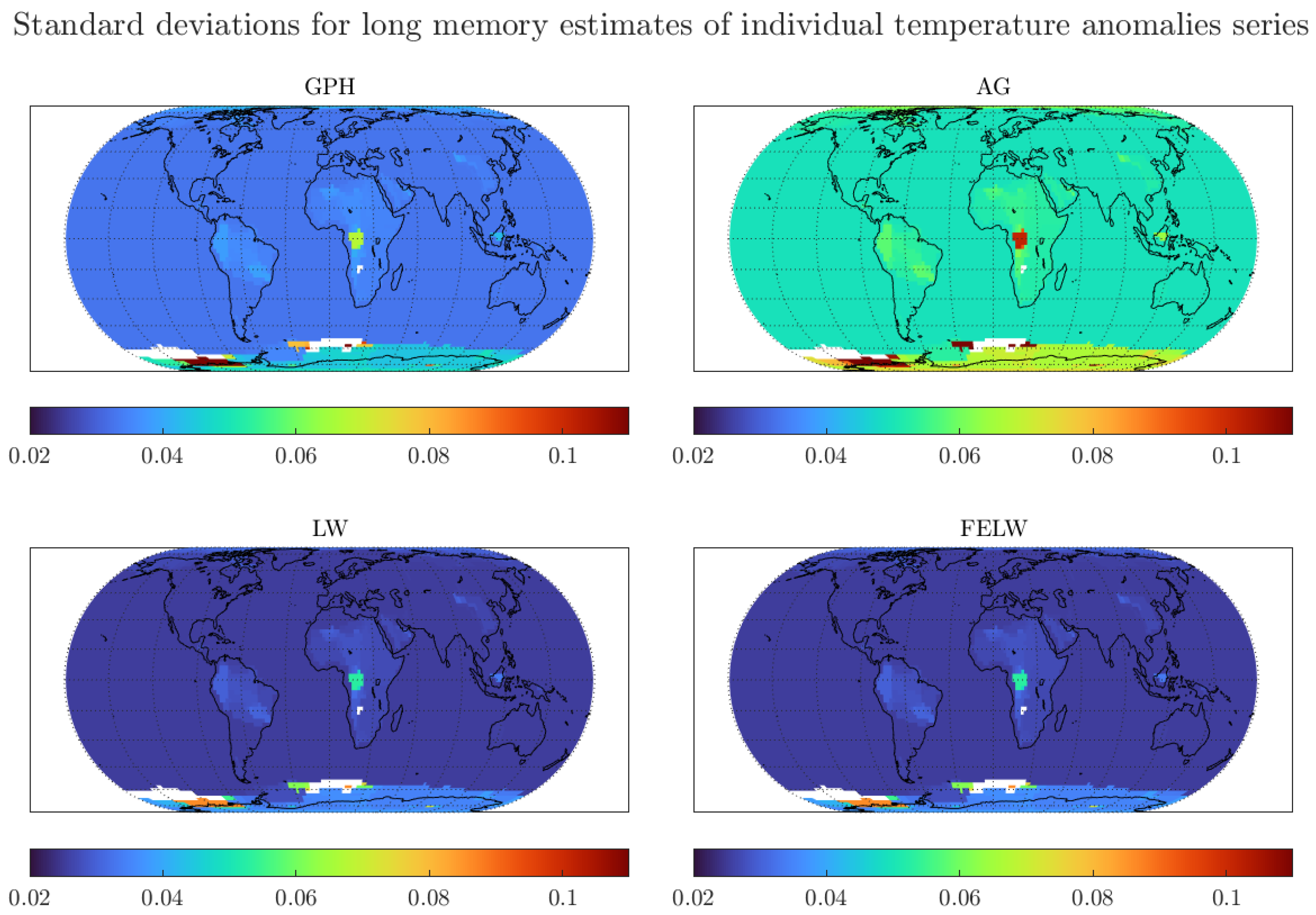
Figure A4.
Standard deviations for long memory estimates of monthly individual grid observations of temperature anomalies. We use the optimal bandwidth and the 250 km smoothing radius dataset.
Figure A4.
Standard deviations for long memory estimates of monthly individual grid observations of temperature anomalies. We use the optimal bandwidth and the 250 km smoothing radius dataset.
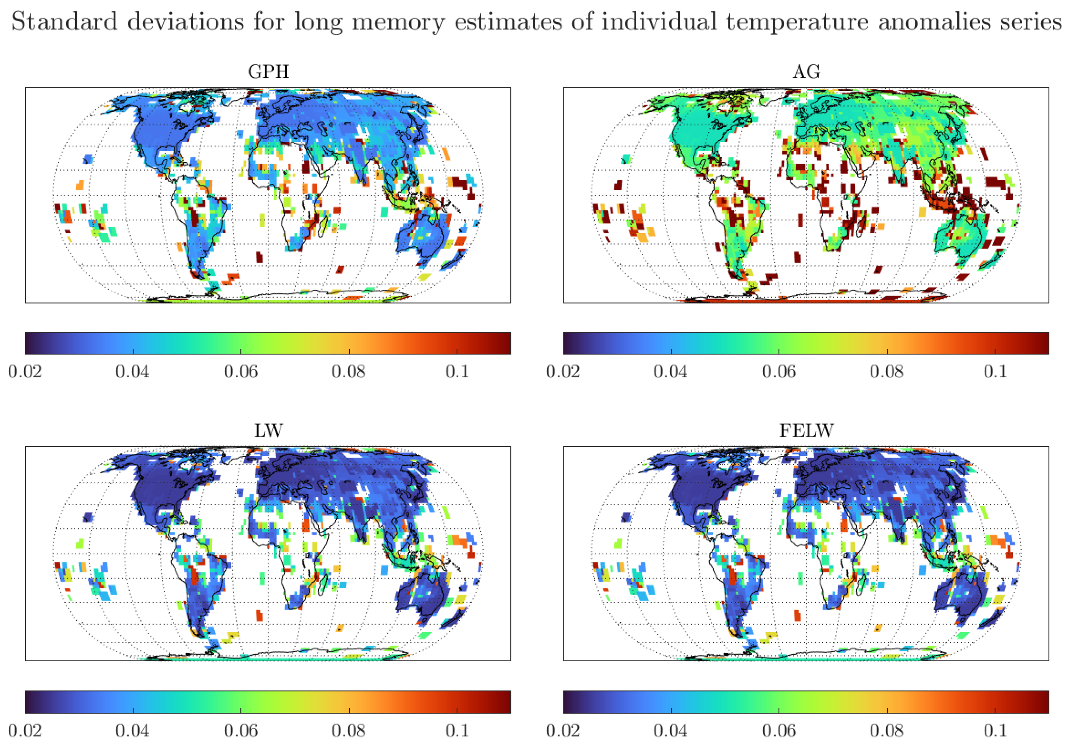
Figure A5.
Histograms and probability density estimates of long memory estimates for monthly individual grid observations of temperature anomalies. We use the optimal bandwidth, the 1200 km smoothing radius dataset, and the GPH estimator.
Figure A5.
Histograms and probability density estimates of long memory estimates for monthly individual grid observations of temperature anomalies. We use the optimal bandwidth, the 1200 km smoothing radius dataset, and the GPH estimator.

Figure A6.
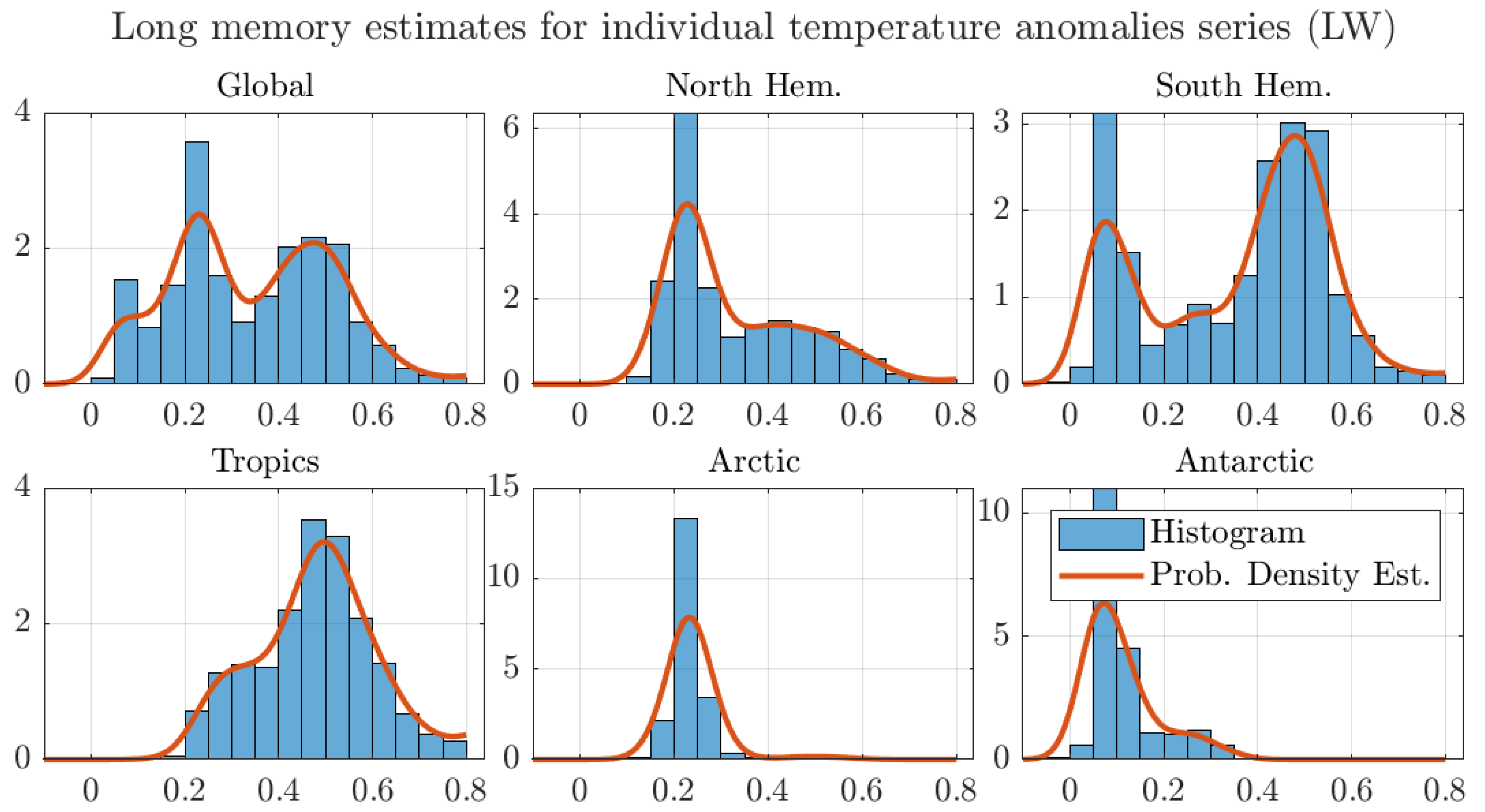
Histograms and probability density estimates of long memory estimates for monthly individual grid observations of temperature anomalies. We use the optimal bandwidth, the 1200 km smoothing radius dataset, and the LW estimator.
Figure A6.
Histograms and probability density estimates of long memory estimates for monthly individual grid observations of temperature anomalies. We use the optimal bandwidth, the 1200 km smoothing radius dataset, and the LW estimator.

Figure A7.
Histograms and probability density estimates of long memory estimates for monthly individual grid observations of temperature anomalies. We use the optimal bandwidth, the 1200 km smoothing radius dataset, and the FELW estimator.
Figure A7.
Histograms and probability density estimates of long memory estimates for monthly individual grid observations of temperature anomalies. We use the optimal bandwidth, the 1200 km smoothing radius dataset, and the FELW estimator.
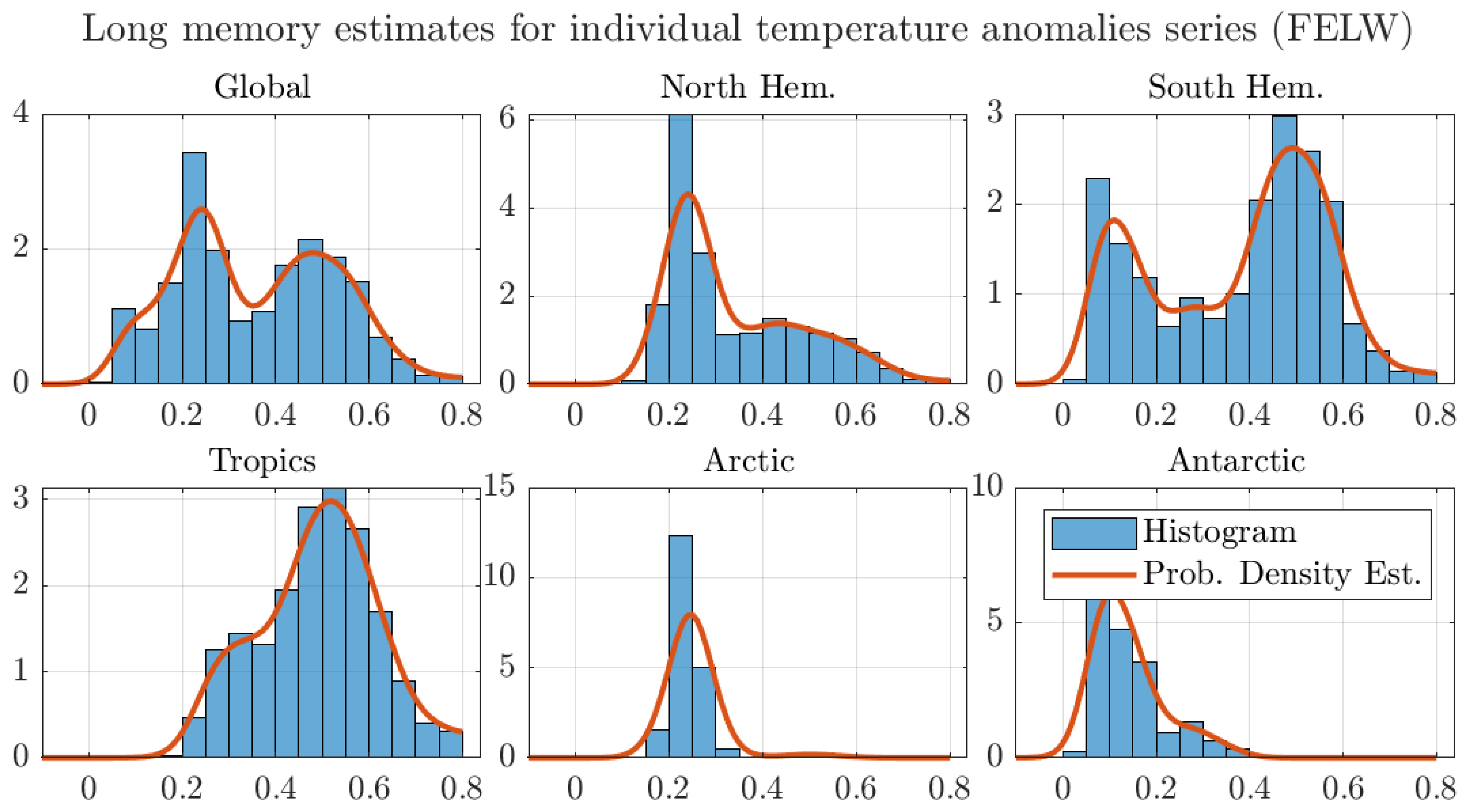
Figure A8.
Histograms and probability density estimates of long memory estimates for monthly individual grid observations of temperature anomalies. We use the optimal bandwidth, the 250 km smoothing radius dataset, and the AG estimator.
Figure A8.
Histograms and probability density estimates of long memory estimates for monthly individual grid observations of temperature anomalies. We use the optimal bandwidth, the 250 km smoothing radius dataset, and the AG estimator.

Figure A9.
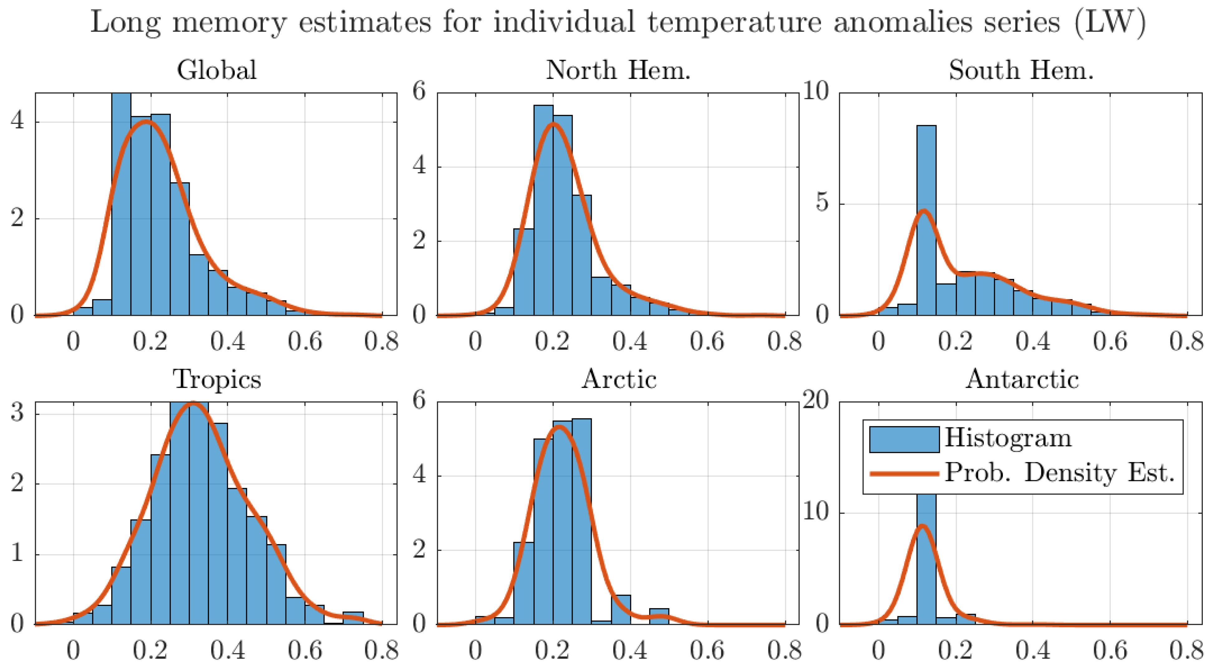
Histograms and probability density estimates of long memory estimates for monthly individual grid observations of temperature anomalies. We use the optimal bandwidth, the 250 km smoothing radius dataset, and the LW estimator.
Figure A9.
Histograms and probability density estimates of long memory estimates for monthly individual grid observations of temperature anomalies. We use the optimal bandwidth, the 250 km smoothing radius dataset, and the LW estimator.

Figure A10.
Histograms and probability density estimates of long memory estimates for monthly individual grid observations of temperature anomalies. We use the optimal bandwidth, the 250 km smoothing radius dataset, and the FELW estimator.
Figure A10.
Histograms and probability density estimates of long memory estimates for monthly individual grid observations of temperature anomalies. We use the optimal bandwidth, the 250 km smoothing radius dataset, and the FELW estimator.
References
- Altissimo, Filippo, Benoit Mojon, and Paolo Zaffaroni. 2009. Can Aggregation Explain the Persistence of Inflation? Journal of Monetary Economics 5: 231–41. [Google Scholar] [CrossRef]
- Andrews, Donald W. K., and Patrik Guggenberger. 2003. A Bias-Reduced Log-Periodogram Regression Estimator For The Long-Memory Parameter. Econometrica 71: 675–712. [Google Scholar] [CrossRef]
- Baillie, Richard T., and Sang Kuck Chung. 2002. Modeling and forecasting from trend-stationary long memory models with applications to climatology. International Journal of Forecasting 18: 215–26. [Google Scholar] [CrossRef]
- Balcilar, Mehmet. 2004. Persistence in Inflation: Does Aggregation Cause Long Memory? Emerging Markets Finance and Trade 40: 25–56. [Google Scholar] [CrossRef]
- Bloomfield, Peter. 1992. Trends in global temperature. Climatic Change 21: 1–16. [Google Scholar] [CrossRef]
- Bloomfield, Peter, and Douglas Nychka. 1992. Climate spectra and detecting climate change. Climatic Change 21: 275–87. [Google Scholar] [CrossRef]
- Calel, Raphael, Sandra C. Chapman, David A. Stainforth, and Nicholas W. Watkins. 2020. Temperature variability implies greater economic damages from climate change. Nature Communications 11: 1–5. [Google Scholar] [CrossRef]
- Diebold, Francis X., and Glenn D Rudebusch. 1989. Long Memory and Persistence in Agregate Output. Journal of Monetary Economics 24: 189–209. [Google Scholar] [CrossRef] [Green Version]
- Geweke, John, and Susan Porter-Hudak. 1983. The Estimation and Application of Long Memory Time Series Models. Journal of Time Series Analysis 4: 221–38. [Google Scholar] [CrossRef]
- Gil-Alana, Luis A. 2005. Statistical modeling of the temperatures in the Northern Hemisphere using fractional integration techniques. Journal of Climate 18: 5357–69. [Google Scholar] [CrossRef]
- GISTEMP Team. 2020. GISS Surface Temperature Analysis (GISTEMP), Version 4. NASA Goddard Institute for Space Studies. Available online: https://data.giss.nasa.gov/gistemp/ (accessed on 10 October 2020).
- Granger, Clive W. J. 1966. The Typical Spectral Shape of an Economic Variable. Econometrica 34: 150–61. [Google Scholar] [CrossRef]
- Granger, Clive W. J. 1980. Long Memory Relationships and the Aggregation of Dynamic Models. Journal of Econometrics 14: 227–38. [Google Scholar] [CrossRef]
- Granger, Clive W. J., and Roselyne Joyeux. 1980. An Introduction to Long Memory Time Series Models and Fractional Differencing. Journal of Time Series Analysis 1: 15–29. [Google Scholar] [CrossRef]
- Haldrup, Niels, and J. Eduardo Vera-Valdés. 2017. Long Memory, Fractional Integration, and Cross-Sectional Aggregation. Journal of Econometrics 199: 1–11. [Google Scholar] [CrossRef] [Green Version]
- Hansen, James, Reto Ruedy, Mki Sato, and Ken Lo. 2010. Global surface temperature change. Reviews of Geophysics 48: 29. [Google Scholar] [CrossRef] [Green Version]
- Hosking, Jonathan R. M. 1981. Fractional Differencing. Biometrika 68: 165–76. [Google Scholar] [CrossRef]
- Hurst, Harold E. 1956. The Problem of Long-Term Storage in Reservoirs. Hydrological Sciences Journal 1: 13–27. [Google Scholar] [CrossRef] [Green Version]
- Hurvich, Clifford M., Rohit Deo, and Julia Brodsky. 1998. The Mean Squared Error of Geweke and Porter-Hudak’s Estimator of the Memory Parameter of a Long-Memory Time Series. Journal of Time Series Analysis 19: 19–46. [Google Scholar] [CrossRef]
- Künsch, Hans. 1987. Statistical Aspects of Self-Similar Processes. Bernouli 1: 67–74. [Google Scholar]
- Lenssen, Nathan J. L., Gavin A. Schmidt, James E. Hansen, Matthew J. Menne, Avraham Persin, Reto Ruedy, and Daniel Zyss. 2019. Improvements in the GISTEMP Uncertainty Model. Journal of Geophysical Research: Atmospheres 124: 6307–26. [Google Scholar] [CrossRef]
- Linden, Mikael. 1999. Time Series Properties of Aggregated AR(1) Processes with Uniformly Distributed Coefficients. Economics Letters 64: 31–36. [Google Scholar] [CrossRef]
- Mandelbrot, Benoit B. 1967. How Long Is the Coast of Britain? Statistical Self-Similarity and Fractional Dimension. Science 156: 636–38. [Google Scholar] [CrossRef] [PubMed] [Green Version]
- Mandelbrot, Benoit B., and John W. Van Ness. 1968. Fractional Brownian Motions, Fractional Noises and Applications. SIAM Review 10: 422–37. [Google Scholar] [CrossRef]
- Mangat, Manveer Kaur, and Erhard Reschenhofer. 2020. Frequency-Domain Evidence for Climate Change. Econometrics 8: 28. [Google Scholar] [CrossRef]
- Marmol, Francesc. 1995. Spurious regressions between I (d) processes. Journal of Time Series Analysis 16: 313–21. [Google Scholar] [CrossRef]
- Mills, Terence C. 2007. Time series modelling of two millennia of northern hemisphere temperatures: Long memory or shifting trends? Journal of the Royal Statistical Society. Series A: Statistics in Society 170: 83–94. [Google Scholar] [CrossRef]
- Oppenheim, Georges, and Marie Claude Viano. 2004. Aggregation of Random Parameters Ornstein-Uhlenbeck or AR Processes: Some Convergence Results. Journal of Time Series Analysis 25: 335–50. [Google Scholar] [CrossRef]
- Osterrieder, Daniela, Daniel Ventosa-Santaulària, and J. Eduardo Vera-Valdés. 2019. The VIX, the Variance Premium, and Expected Returns. Journal of Financial Econometrics 17: 517–58. [Google Scholar] [CrossRef] [Green Version]
- Peterson, Thomas C., and Russell S. Vose. 1997. An overview of the global historical climatology network temperature database. Bulletin of the American Meteorological Society 78: 2837–50. [Google Scholar] [CrossRef] [Green Version]
- Phillips, Peter C.B., and Katsumi Shimotsu. 2004. Local whittle estimation in nonstationary and unit root cases. Annals of Statistics 32: 656–92. [Google Scholar] [CrossRef] [Green Version]
- Reschenhofer, Erhard, and Manveer Kaur Mangat. 2020. Detecting long-range dependence with truncated ratios of periodogram ordinates. Communications in Statistics—Theory and Methods 17: 1–16. [Google Scholar] [CrossRef] [Green Version]
- Robinson, Peter M. 1995a. Gaussian Semiparametric Estimation of Long Range Dependence. The Annals of Statistics 23: 1630–61. [Google Scholar] [CrossRef]
- Robinson, Peter M. 1995b. Log-Periodogram Regression of Time Series with Long Range Dependence. The Annals of Statistics 23: 1048–72. [Google Scholar] [CrossRef]
- Shimotsu, Katsumi, and Peter C.B. Phillips. 2005. Exact Local Whittle Estimation of Fractional Integration. The Annals of Statistics 33: 1890–933. [Google Scholar] [CrossRef] [Green Version]
- Shimotsu, Katsumi. 2010. Exact local Whittle estimation of fractional integration with unknown mean and time trend. Econometric Theory 26: 501–40. [Google Scholar] [CrossRef] [Green Version]
- Sutton, Rowan T., Buwen Dong, and Jonathan M. Gregory. 2007. Land/sea warming ratio in response to climate change: IPCC AR4 model results and comparison with observations. Geophysical Research Letters 34: 1–5. [Google Scholar] [CrossRef]
- Tsay, Wen-Jen, and Ching-Fan Chung. 2000. The spurious regression of fractionally integrated processes. Journal of Econometrics 96: 155–82. [Google Scholar] [CrossRef]
- Velasco, Carlos. 1999a. Gaussian semiparametric estimation of non-stationary time series. Journal of Time Series Analysis 20: 87–127. [Google Scholar] [CrossRef] [Green Version]
- Velasco, Carlos. 1999b. Non-stationary log-periodogram regression. Journal of Econometrics 91: 325–71. [Google Scholar] [CrossRef] [Green Version]
- Velasco, Carlos. 2000. Non-Gaussian Log-Periodogram Regression. Econometric Theory 16: 44–79. [Google Scholar] [CrossRef] [Green Version]
- Ventosa-Santaulària, Daniel, J. Eduardo Vera-Valdés, Katarzyna Łasak, and Ricardo Ramírez-Vargas. 2020. Spurious multivariate regressions under fractionally integrated processes. Communications in Statistics—Theory and Methods 6: 1–23. [Google Scholar] [CrossRef]
- Vera-Valdés, J. Eduardo. 2020. On long memory origins and forecast horizons. Journal of Forecasting 39: 811–26. [Google Scholar] [CrossRef] [Green Version]
- Zaffaroni, Paolo. 2004. Contemporaneous Aggregation of Linear Dynamic Models in Large Economies. Journal of Econometrics 120: 75–102. [Google Scholar] [CrossRef]
Figure 1.
Author’s own plot with data from Goddard Institute for Space Studies Surface Temperature Analysis (GISTEMP). Smoothing radius of 1200 km.
Figure 1.
Author’s own plot with data from Goddard Institute for Space Studies Surface Temperature Analysis (GISTEMP). Smoothing radius of 1200 km.
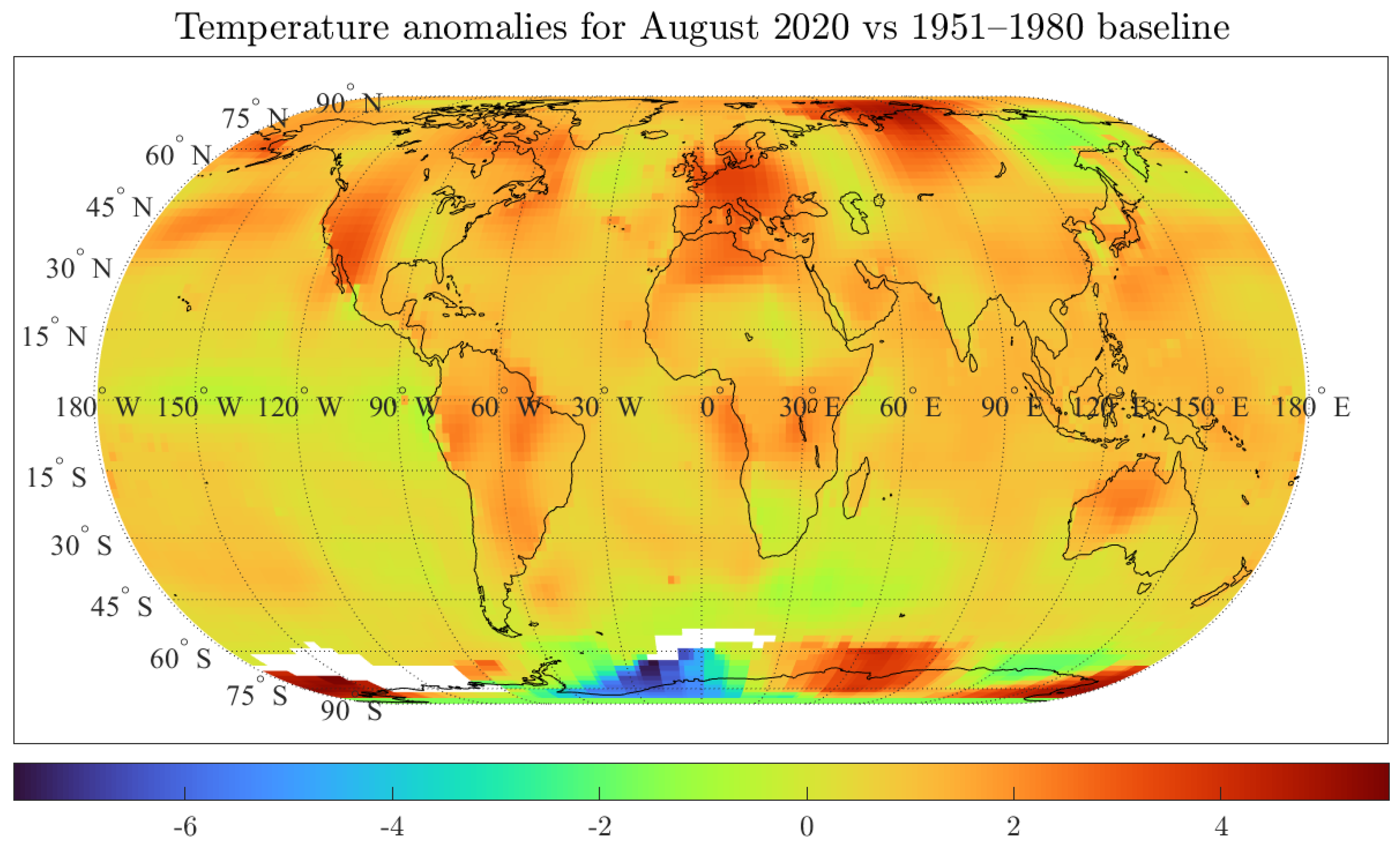
Figure 2.
Temperature anomalies for monthly regional temperatures presented by GISTEMP. For illustrative purposes, the temperature reported near London (,) is also shown.
Figure 2.
Temperature anomalies for monthly regional temperatures presented by GISTEMP. For illustrative purposes, the temperature reported near London (,) is also shown.

Figure 3.
Sample autocorrelation functions for monthly regional temperatures presented by GISTEMP. The autocorrelation function for the temperature reported near London (,) is also shown. The shaded area covers from the first to the third quartile of the autocorrelation functions of the individual grid series.
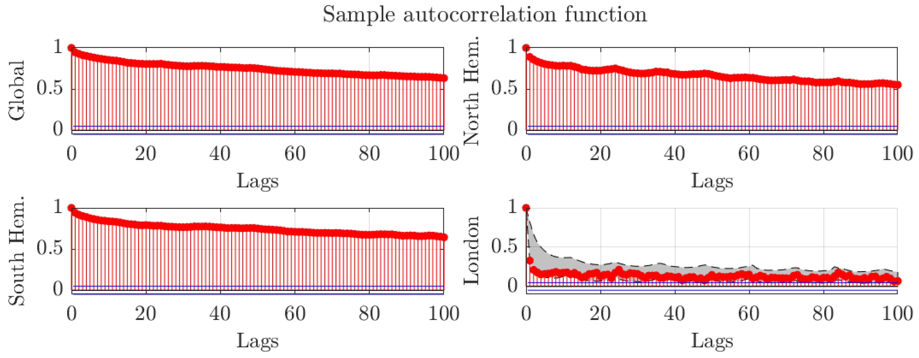
Figure 4.
Autocorrelation functions for individual AR(1) processes with different autoregressive coefficient. Also shown, the autocorrelation function of the aggregated process.
Figure 4.
Autocorrelation functions for individual AR(1) processes with different autoregressive coefficient. Also shown, the autocorrelation function of the aggregated process.

Figure 5.
Long memory estimates for monthly individual grid observations of temperature anomalies. We use the optimal bandwidth and the 1200 km smoothing radius dataset. GPH: Log-periodogram regression, AG: Andrews and Guggenberger (2003) estimator, LW: Local Whittle estimator, and FELW: Feasible exact local Whittle.
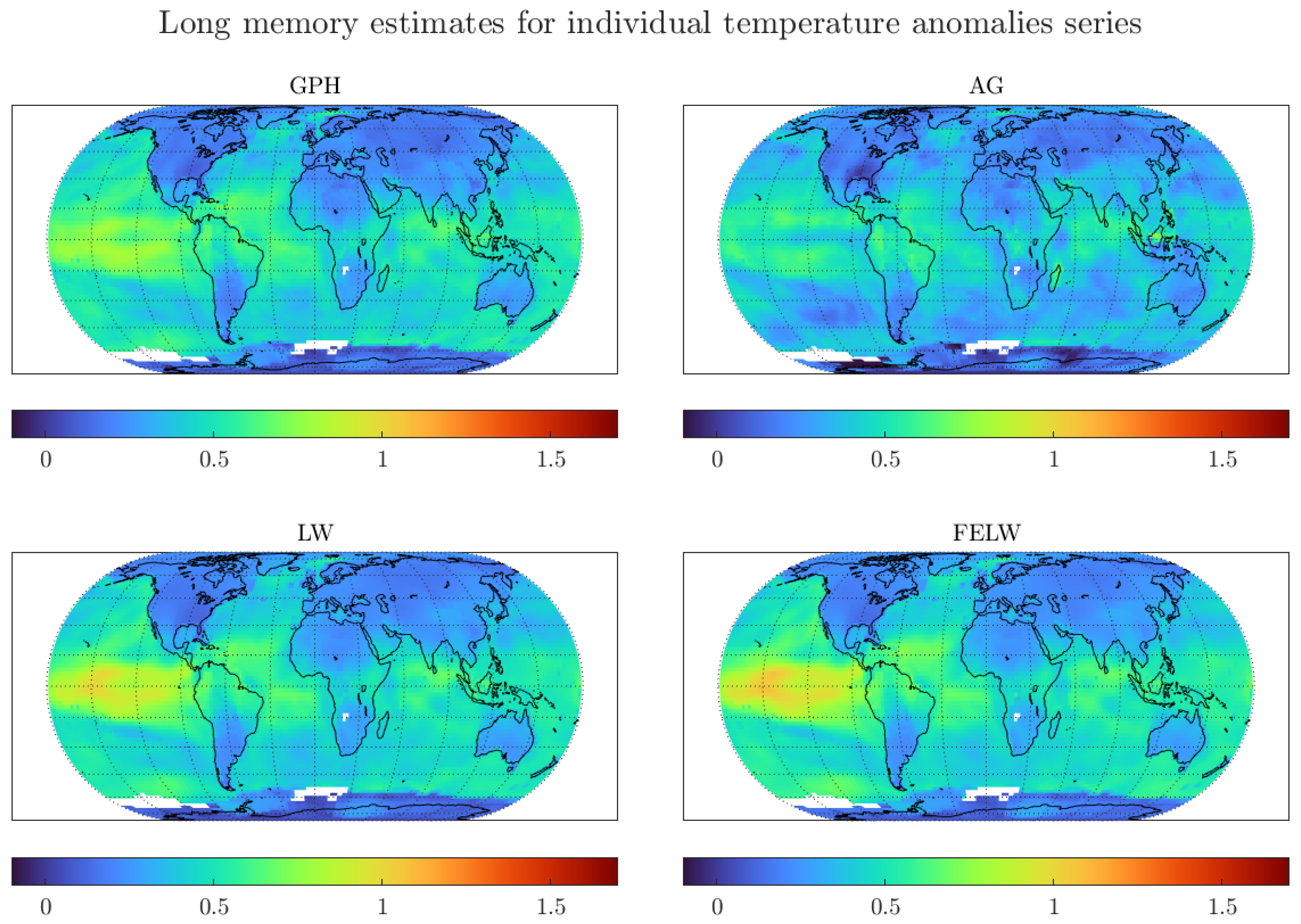
Figure 6.
Histograms and probability density estimates of long memory estimates for monthly individual grid observations of temperature anomalies. We use the optimal bandwidth, the 1200 km smoothing radius dataset, and the Andrews and Guggenberger (2003) (AG) estimator.
Figure 6.
Histograms and probability density estimates of long memory estimates for monthly individual grid observations of temperature anomalies. We use the optimal bandwidth, the 1200 km smoothing radius dataset, and the Andrews and Guggenberger (2003) (AG) estimator.

Figure 7.
Long memory estimates for monthly individual grid observations of temperature anomalies. We use the optimal bandwidth and the 250 km smoothing radius dataset.
Figure 7.
Long memory estimates for monthly individual grid observations of temperature anomalies. We use the optimal bandwidth and the 250 km smoothing radius dataset.
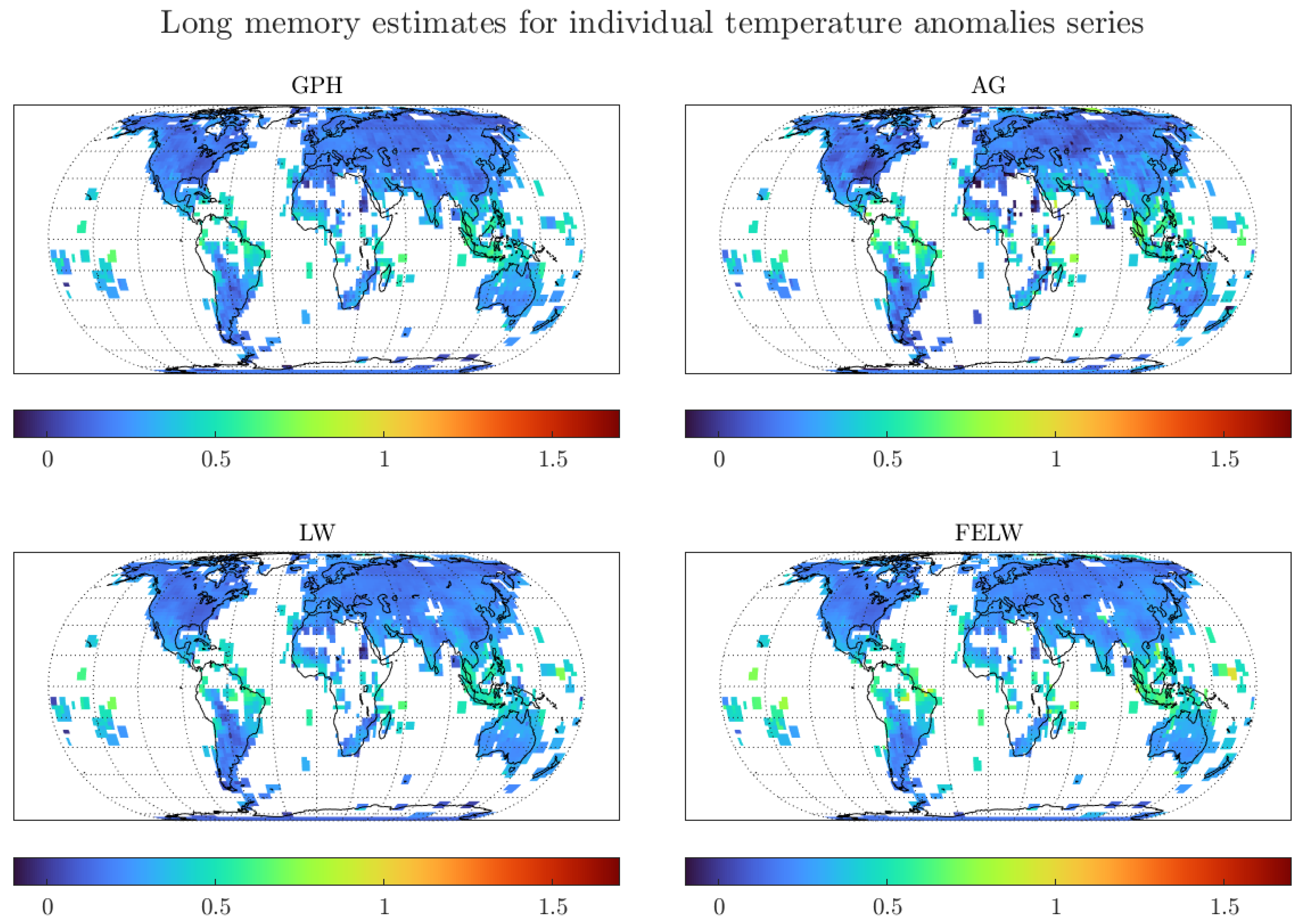
Figure 8.
Histograms and probability density estimates of long memory estimates for monthly individual grid observations of temperature anomalies. We use the optimal bandwidth, the 250 km smoothing radius dataset, and the log-periodogram regression (GPH) estimator.
Figure 8.
Histograms and probability density estimates of long memory estimates for monthly individual grid observations of temperature anomalies. We use the optimal bandwidth, the 250 km smoothing radius dataset, and the log-periodogram regression (GPH) estimator.

Table 1.
Long memory estimates for monthly regional temperature anomalies using the optimal bandwidth. For the London grid, we use the 1200 km smoothing radius dataset. * Note that all series have equal sample sizes so that the estimates share the same standard deviations.
Table 1.
Long memory estimates for monthly regional temperature anomalies using the optimal bandwidth. For the London grid, we use the 1200 km smoothing radius dataset. * Note that all series have equal sample sizes so that the estimates share the same standard deviations.
| Series | GPH | AG | LW | FELW | Sample Size |
|---|---|---|---|---|---|
| Global | 0.6332 | 0.7475 | 0.6682 | 0.6304 | 1688 |
| North Hem. | 0.5429 | 0.6247 | 0.5765 | 0.5584 | 1688 |
| South Hem. | 0.6407 | 0.6904 | 0.6430 | 0.6159 | 1688 |
| London (,) | 0.2346 | 0.2388 | 0.2288 | 0.2354 | 1688 |
| Std. Dev. * | (0.0328) | (0.0492) | (0.0256) | (0.0256) |
Table 2.
Regional long memory averages for monthly temperature anomalies. We use the optimal bandwidth and the 1200 km smoothing radius dataset. The bar on top denotes averages. Standard deviations given the average sample sizes are given below between parentheses.
Table 2.
Regional long memory averages for monthly temperature anomalies. We use the optimal bandwidth and the 1200 km smoothing radius dataset. The bar on top denotes averages. Standard deviations given the average sample sizes are given below between parentheses.
| Series | GPH | AG | LW | FELW | No. of Grids | |
|---|---|---|---|---|---|---|
| 0.3427 | 0.2951 | 0.3540 | 0.3738 | 1463 | 15,981 | |
| (0.0347) | (0.0521) | (0.0271) | (0.0271) | |||
| 0.3236 | 0.3082 | 0.3389 | 0.3539 | 1560 | 8100 | |
| (0.0338) | (0.0508) | (0.0264) | (0.0264) | |||
| 0.3624 | 0.2817 | 0.3695 | 0.3942 | 1364 | 7881 | |
| (0.0357) | (0.0536) | (0.0279) | (0.0279) | |||
| 0.4855 | 0.4103 | 0.5019 | 0.5216 | 1642 | 5397 | |
| (0.0332) | (0.0497) | (0.0259) | (0.0259) | |||
| 0.2164 | 0.2588 | 0.2404 | 0.2525 | 1286 | 2160 | |
| (0.0366) | (0.0549) | (0.0285) | (0.0285) | |||
| 0.1174 | 0.0874 | 0.1084 | 0.1401 | 681 | 2090 | |
| (0.0471) | (0.0707) | (0.0368) | (0.0368) |
Table 3.
Regional long memory averages for monthly temperature anomalies. We use the optimal bandwidth and the 250 km smoothing radius dataset. The bar on top denotes averages. Standard deviations given the average sample sizes are given below between parentheses.
Table 3.
Regional long memory averages for monthly temperature anomalies. We use the optimal bandwidth and the 250 km smoothing radius dataset. The bar on top denotes averages. Standard deviations given the average sample sizes are given below between parentheses.
| Series | GPH | AG | LW | FELW | No. of Grids | |
|---|---|---|---|---|---|---|
| 0.2279 | 0.2406 | 0.2277 | 0.2626 | 895 | 6185 | |
| (0.0423) | (0.0634) | (0.0330) | (0.0330) | |||
| 0.2179 | 0.2286 | 0.2315 | 0.2596 | 1106 | 3927 | |
| (0.0389) | (0.0583) | (0.0303) | (0.0303) | |||
| 0.2452 | 0.2615 | 0.2209 | 0.2678 | 528 | 2258 | |
| (0.0522) | (0.0783) | (0.0407) | (0.0407) | |||
| 0.3308 | 0.3406 | 0.3315 | 0.3786 | 732 | 1685 | |
| (0.0458) | (0.0687) | (0.0357) | (0.0357) | |||
| 0.2009 | 0.2259 | 0.2248 | 0.2678 | 845 | 797 | |
| (0.0432) | (0.0649) | (0.0337) | (0.0337) | |||
| 0.1680 | 0.2005 | 0.1205 | 0.1633 | 284 | 1070 | |
| (0.0669) | (0.1003) | (0.0521) | (0.0521) |
Table 4.
Regional long memory averages for yearly temperature anomalies. We use the optimal bandwidth and the 250 km smoothing radius dataset. The bar on top denotes averages. Standard deviations given the average sample sizes are given below between parentheses.
Table 4.
Regional long memory averages for yearly temperature anomalies. We use the optimal bandwidth and the 250 km smoothing radius dataset. The bar on top denotes averages. Standard deviations given the average sample sizes are given below between parentheses.
| Series | GPH | AG | LW | FELW | No. of Grids | |
|---|---|---|---|---|---|---|
| 0.4051 | 0.4278 | 0.3458 | 0.5573 | 78 | 6006 | |
| (0.1116) | (0.1674) | (0.0870) | (0.0870) | |||
| 0.3784 | 0.5079 | 0.3621 | 0.5218 | 94 | 3982 | |
| (0.1040) | (0.1560) | (0.0811) | (0.0811) | |||
| 0.4542 | 0.2802 | 0.3159 | 0.6225 | 47 | 2114 | |
| (0.1367) | (0.2051) | (0.1066) | (0.1066) | |||
| 0.4621 | 0.5088 | 0.4074 | 0.6608 | 66 | 1563 | |
| (0.1191) | (0.1786) | (0.0928) | (0.0928) | |||
| 0.3166 | 0.4880 | 0.3083 | 0.4939 | 77 | 761 | |
| (0.1134) | (0.1700) | (0.0884) | (0.0884) | |||
| 0.4682 | 0.1177 | 0.2578 | 0.6449 | 24 | 1059 | |
| (0.1779) | (0.2668) | (0.1387) | (0.1387) |
Table 5.
Regional long memory averages for yearly temperature anomalies. The bandwidth is given by , with T the sample size. We use the 250 km smoothing radius dataset. The bar on top denotes averages.
Table 5.
Regional long memory averages for yearly temperature anomalies. The bandwidth is given by , with T the sample size. We use the 250 km smoothing radius dataset. The bar on top denotes averages.
| Series | GPH | AG | LW | FELW | No. of Grids | |
|---|---|---|---|---|---|---|
| 0.5947 | 0.8443 | 0.5343 | 0.6429 | 78 | 6006 | |
| (0.2138) | (0.3206) | (0.1667) | (0.1667) | |||
| 0.6276 | 1.0159 | 0.5650 | 0.6364 | 94 | 3982 | |
| (0.2028) | (0.3042) | (0.1581) | (0.1581) | |||
| 0.5342 | 0.5284 | 0.4777 | 0.6549 | 47 | 2114 | |
| (0.2424) | (0.3636) | (0.1890) | (0.1890) | |||
| 0.6718 | 0.8727 | 0.6115 | 0.6725 | 66 | 1563 | |
| (0.2267) | (0.3401) | (0.1768) | (0.1768) | |||
| 0.5528 | 1.2723 | 0.4883 | 0.5924 | 77 | 761 | |
| (0.2138) | (0.3206) | (0.1667) | (0.1667) | |||
| 0.4133 | 0.4156 | 0.3766 | 0.6872 | 24 | 1059 | |
| (0.2868) | (0.4302) | (0.2236) | (0.2236) |
Publisher’s Note: MDPI stays neutral with regard to jurisdictional claims in published maps and institutional affiliations. |
© 2021 by the author. Licensee MDPI, Basel, Switzerland. This article is an open access article distributed under the terms and conditions of the Creative Commons Attribution (CC BY) license (http://creativecommons.org/licenses/by/4.0/).
Share and Cite
MDPI and ACS Style
Vera-Valdés, J.E. Temperature Anomalies, Long Memory, and Aggregation. Econometrics 2021, 9, 9. https://0-doi-org.brum.beds.ac.uk/10.3390/econometrics9010009
AMA Style
Vera-Valdés JE. Temperature Anomalies, Long Memory, and Aggregation. Econometrics. 2021; 9(1):9. https://0-doi-org.brum.beds.ac.uk/10.3390/econometrics9010009
Chicago/Turabian StyleVera-Valdés, J. Eduardo. 2021. "Temperature Anomalies, Long Memory, and Aggregation" Econometrics 9, no. 1: 9. https://0-doi-org.brum.beds.ac.uk/10.3390/econometrics9010009
Note that from the first issue of 2016, this journal uses article numbers instead of page numbers. See further details here.