Quantile Regression with Generated Regressors

Abstract

This paper studies estimation and inference for linear quantile regression models with generated regressors. We suggest a practical two-step estimation procedure, where the generated regressors are computed in the first step. The asymptotic properties of the two-step estimator, namely, consistency and asymptotic normality are established. We show that the asymptotic variance-covariance matrix needs to be adjusted to account for the first-step estimation error. We propose a general estimator for the asymptotic variance-covariance, establish its consistency, and develop testing procedures for linear hypotheses in these models. Monte Carlo simulations to evaluate the finite-sample performance of the estimation and inference procedures are provided. Finally, we apply the proposed methods to study Engel curves for various commodities using data from the UK Family Expenditure Survey. We document strong heterogeneity in the estimated Engel curves along the conditional distribution of the budget share of each commodity. The empirical application also emphasizes that correctly estimating confidence intervals for the estimated Engel curves by the proposed estimator is of importance for inference.

1. Introduction

Since the seminal work of Koenker and Bassett (1978), quantile regression (QR) models have provided a valuable tool in economics, finance, and statistics as a way of capturing heterogeneous effects of covariates on the outcome of interest, exposing a wide variety of forms of conditional heterogeneity under weak distributional assumptions. Importantly, QR also provides a framework for robust inference.

Applied researchers are commonly confronted with the absence of observable regressors in practice. In some cases, proxies for the unobservable variables can be found in data, while in other cases, these regressors need to be estimated. Thus, a very common strategy to deal with unobservable variables is to replace them with estimated values, that is, generated regressors (GRs).1 These GRs have important implications for the reliability of general standard estimation and inference procedures. Pagan (1984) and Murphy and Topel (2002) point out that even though consistent estimates of parameters of interest are produced when the unobserved regressors are replaced with their estimated values, the conventional ways to estimate standard errors are incorrect. Recently, Mammen et al. (2012) provide a general theory for the impact of GRs on the final estimator’s asymptotic properties in nonparametric mean regression. Hahn and Rider (2013) derive the asymptotic distribution of three-step estimators of a finite-dimensional parameter in a semiparametric mean regression models where GR is estimated parametrically or nonparametrically in the first-step.

A number of important statistical applications requires estimation of a conditional quantile function when some of the covariates are not directly observed, but are estimated in a preliminary step. Examples include, among others, stochastic volatility time-series models, triangular simultaneous equation models, censoring, sample selection models, and treatment effects models.2

This paper contributes to the literature by systematically studying and formalizing estimation and inference for linear QR models with a general semiparametric GR. The main contributions are as following. First, we suggest a practical two-step estimation procedure to estimate the parameters of interest in the QR-GR model. The first-step applies a general (semi)-parametric estimator to compute the GRs. The second step uses the GRs as regressor variables in a QR estimation. We establish the asymptotic properties of the two-step QR-GR estimator, namely, consistency and asymptotic normality. We show that the asymptotic variance-covariance matrix needs to be adjusted to account for the first-step estimation error. The basic idea is as follows. Since the first-step estimation of the unobservable regressors produces consistent estimates of the corresponding true parameters, the GRs are consistently estimated. However, the GR are included in the QR model of interest with sampling error, which introduces additional noise into the asymptotic variance-covariance matrix of the coefficients of interest. In other words, the sampling error from the first stage contaminates the second stage estimation. Therefore, the usual way of calculating the QR variance-covariance matrix fails to account for the additional source of error. Under some general conditions, the estimated limiting distribution of the first-step is used to consistently estimate the variance-covariance matrix of the parameters of interest.

The second contribution of the paper is to develop inference procedures for the QR model with GR. Though estimation and inference for conditional average models with GR have been widely studied and used in practice, the literature on QR with GR is more sparse. We develop testing procedures for general linear hypotheses in these models based on Wald-type tests, and derive their associated limiting distributions. To implement the tests, we propose an estimator for the asymptotic variance-covariance of the QR-GR coefficients, and formally establish its consistency. An important advantage of the proposed tests is that they are simple to compute and implement in practice.

Compared to the existing procedures, the QR-GR methods proposed in this paper present several distinctive advantages for applied researchers. First, instead of imposing a linear structure in the first step, as in Xiao and Koenker (2009), or imposing triangular structure between two steps, as in Ma and Koenker (2006) and Lee (2007), we work with the general case of QR-GR where no structural restrictions between the two steps or any specific functional forms and estimation strategies in the first step are imposed. That is useful in applied work since practitioners have a large range of alternatives to construct the unobservable variables by using different estimation strategies or even different data sets. Second, we establish the asymptotic properties of the QR-GR estimator for non-iid data under weak conditions. This is an important generalization for practitioners since it allows for inference in a more general class of models. Third, we develop practical inference procedures. Finally, the weak conditions we imposed for QR-GR allow for simple computational implementation.3 Linear QR models have been the workhorse of the applied research and the methods lead to a simple algorithm that can be conveniently implemented in empirical applications. Researchers can simply use existing software packages for the first-step estimation and to construct the regressors needed, for example, MLE, OLS, QR or GMM, and then apply the QR procedure with our described variance-covariance matrix adjustment.

Monte Carlo simulations assess the finite-sample properties of the proposed methods. We evaluate the QR-GR estimator in terms of empirical bias and root mean squared error, and compare its performance with methods that are not designed for dealing with GR issues. In addition, we compute the corresponding standard errors of the QR-GR estimator and evaluate its bias. The experiments suggest that the proposed approach performs very well in finite samples and effectively removes the bias of the standard errors induced by the GR. Thus, the proposed variance estimator is approximately unbiased and approximates well the true variance.

Finally, to motivate and illustrate the applicability of the methods, we consider an empirical application to study demand models, using data from the UK Family Expenditure Survey. Demand models (also known as Engel curves) represent the relationship between total expenditure and the share of various commodities to total expenditure. The QR approach is a useful tool in this example because it allows us to capture the heterogeneity in the expenditures of the different commodities along the conditional distribution of each commodity share. The first step in this exercise is to estimate the unobserved motives for budget shares of different commodities using the factor analysis proposed by Barigozzi and Moneta (2016). The unobserved factors consist of the motives of consumption as necessities, luxuries, and unitary elasticity goods. In the second step, we apply the proposed QR-GR estimator to obtain Engel curves for the commodities such as food, housing and leisure, by regressing each commodity share on the estimated motives from the first step. We found that the motives of consumption play different roles for various commodities and contributions of motives to each budget share vary over the total expenditure. Furthermore, the empirical results document important heterogeneity in the Engel curves. The estimated curves present strong heterogenous effect of the consumption motives on the budget share along the conditional distribution of the budget share in most commodities. Importantly, the empirical study underscores the importance of obtaining correct confidence intervals for the estimated Engel curves by taking into account the GR issue.

The remainder of the article is organized as follows. Section 2 introduces the QR model with GR. Section 3 establishes consistency and asymptotic normality of the two-step estimator. Section 4 proposes a consistent estimator of the variance-covariance matrix. Section 5 presents Monte Carlo simulations. Section 6 presents the empirical application to Engel curves. Section 7 concludes the article. Technical proofs are included in the Appendix A.

2. Quantile Regression with Generated Regressors

This section describes the quantile regression (QR) model with generated regressors (GRs) we consider in this paper and the two-step estimation procedure.

2.1. Model

For each fixed $\tau \in (0,1)$, we consider the following model

$$y_i={\mathit{x}}_i^{\top }{\mathbf{\beta }}_0\left(\tau \right)+u_i,i=1,...,n,$$

(1)

where $y_i$ is a response variable, ${\mathit{x}}_i=(x_{i1},\cdots ,x_{ik})$ is a k–dimensional vector of explanatory variables, ${\mathbf{\beta }}_0\left(\tau \right)$ is a $k\times 1$ vector of parameters, and the innovation term $u_i$ has conditional $\tau$-quantile zero, that is $F_{\tau }^{-1}\left(u_i\right|{\mathit{x}}_i)=0$.

When all the regressors ${\mathit{x}}_i$ in model (1) are observable, the model can be written as the following standard QR model

$$Q_{\tau }\left(y_i\right|{\mathit{x}}_i)={\mathit{x}}_i^{\top }{\mathbf{\beta }}_0\left(\tau \right),$$

(2)

where $Q_{\tau }\left(y_i\right|{\mathit{x}}_i)$ is the conditional $\tau$-quantile of $y_i$ given ${\mathit{x}}_i$. In general, ${\mathbf{\beta }}_0$ can depend on $\tau$. The model is semiparametric in the sense that the functional form of the conditional distribution of $y_i$ given ${\mathit{x}}_i$ is left unspecified.

The parameter of interest for the researcher is ${\mathbf{\beta }}_0\left(\tau \right)$ in model (2). However, in many applications one or more elements of the vector of regressors ${\mathit{x}}_i$ may not be directly observable, but instead estimated from a model with other given variables, that is, the GRs. In this paper, we assume that some of the regressors in the vector ${\mathit{x}}_i$ are not observable to the researcher, i.e., $(x_{i1},\cdots ,x_{iq})$ are not directly observable, but $(x_{iq+1},\cdots ,x_{ik})$ are observed, where $q\le k$. In particular, the GR are assumed to have the following form

$$x_{ij}=g_j({\mathit{w}}_i,{\mathbf{\theta }}_j)+v_{ij},$$

where the function $g_j(·,·)$ is differentiable and known up to the unknown $p_j\times 1$ parameter vector $\mathbf{\theta }$ for $j=1,\cdots ,q$, and the variable ${\mathit{w}}_i=(w_{i1},...,w_{iq})$ is a q-dimensional vector of observables, and where $v_{ij}$ is an error term. Thus, one can still estimate the QR model in (2) by replacing $x_{ij}$ with the GR ${\widehat{x}}_{ij}$ for $j=1,\cdots ,q$. The GR ${\widehat{x}}_{ij}$ is obtained from the following first-step estimation

$${\widehat{x}}_{ij}=g_j({\mathit{w}}_i,{\widehat{\mathbf{\theta }}}_j),$$

(3)

where ${\widehat{\mathbf{\theta }}}_j$ satisfies very general weak conditions as: $\sqrt{n}({\widehat{\mathbf{\theta }}}_j-{\mathbf{\theta }}_j)=n^{-1/2}{\sum }_{i=1}^n{\mathit{r}}_i\left({\mathbf{\theta }}_j\right)+o_p\left(1\right)$, and $\mathit{r}(·)$ is a generic function satisfying $E\left[{\mathit{r}}_i\left({\mathbf{\theta }}_j\right)\right]=0$. Equation (3) defines the GR and could be satisfied by different models, we provide a few examples below. Notice that most estimators used in empirical applications satisfy this first-order representation. We will discuss these conditions more formally below. To complete the model, together with (2) and (3), we assume that $F_{\tau }^{-1}\left(u_i\right|{\mathit{w}}_{i1},\cdots ,{\mathit{w}}_{iq},x_{iq+1},\cdots ,x_{ik})=0$.

Remark 1.

One or more elements of the regressors ${\mathit{x}}_i$ may be estimated in the first step. Each of the GRs could be related to different observable variables in different functional forms. For simplicity, each of the GR equations can be estimated separately, and any dependence between the GRs would be captured by the variance covariance matrix.

Remark 2.

We note that the estimation of quantile regression models with mismeasured regressors leads to inconsistent estimates and a few methodologies have been proposed to overcome this drawback (e.g., Wei and Carroll (2009); Wang et al. (2012); Firpo et al. (2017)). Thus, the problem is different from the quantile regression with generated regressors where the standard quantile estimation is still consistent.

To motivate the existence of GRs for QR models, and illustrate how a QR-GR framework could appear in practice, we include the following motivating examples:

Example 1 (Two-stage regression with proxy variables).

A very important example of GR occurs when the variables ${\mathit{x}}_i$ are not directly observable. For instance, assume that the variables $(x_{i1},\cdots ,x_{iq})$ are related to additional observable variables, ${\mathit{w}}_{ij}$, as follows

$$\begin{array}{cc}\hfill {\tilde{x}}_{i1}& =x_{i1}+v_{i1}=g_1({\mathit{w}}_{i1},{\mathbf{\theta }}_{\mathbf{1}})+v_{i1},\hfill \\ \hfill & ⋮\hfill \\ \hfill {\tilde{x}}_{iq}& =x_{iq}+v_{iq}=g_q({\mathit{w}}_{iq},{\mathbf{\theta }}_{\mathbf{q}})+v_{iq}\hfill \end{array}$$

where $({\tilde{x}}_{i1},\cdots ,{\tilde{x}}_{iq})$ are proxy variables, or endogenous observables, ${\mathit{w}}_{ij}$ is a vector of exogenous observable variables, ${\mathbf{\theta }}_j$ is a $p_j\times 1$ vector, the functions $g_j(·)$ are unknown up to the vector ${\mathbf{\theta }}_j$, and $v_{ji}$ are mutually independent innovation terms, for $j=1,\cdots ,q$.

In this case, to complete the definition of the GR one needs to impose more structure on the innovation term $v_{ji}$ to estimate the parameters ${\mathbf{\theta }}_j$, for $j=1,\cdots ,q$. As special cases of a more general procedure which generates the regressors, consider a simple but commonly used linear model to generate one regressor, $x_{i1}$, as a function of several variables ${\mathit{w}}_i$, that is, ${\tilde{x}}_1=g(\mathit{w},\mathbf{\theta })+v={\mathit{w}}^{\top }\mathbf{\theta }+v$. The following are two standard examples.

Example 1.1 (Conditional average). A simple example for the GR model is a linear conditional expectation. In this case, the GR model is defined as

$$E\left[{\tilde{x}}_{i1}\right|{\mathit{w}}_i]={\mathit{w}}_i^{\top }\mathbf{\theta }.$$

Example 1.2 (Conditional quantile). Another simple model for the GR is a linear conditional quantile. In this case, for a given quantile ${\tau }^{\prime }$ specified by the researcher, the GR model is defined as

$$Q_{{\tau }^{\prime }}\left({\tilde{x}}_{i1}\right|{\mathit{w}}_i)={\mathit{w}}_i^{\top }\mathbf{\theta }\left({\tau }^{\prime }\right),$$

In practice one needs to estimate the parameters $\mathbf{\theta }$ in both examples and compute the GR.

Example 2 (Quantile regression with endogeneity: control function approach).

Consider the following model

$$y_i=x_{i1}{\beta }_1+{\mathbf{z}}_i^{\top }{\mathbf{\beta }}_2+u_i$$

(4)

where $x_{i1}$ is the endogenous explanatory variable, ${\beta }_1$ is a scalar parameter for simplicity, and ${\mathbf{z}}_i$ is the $(k-1)\times 1$ vector of exogenous variables, ${\mathbf{\beta }}_2$ is a $(k-1)\times 1$ vector of parameters. Assume that ${\mathit{w}}_{i1}$ are valid instruments. In the control function approach, one could model the endogenous explanatory variable as following:

$$x_{i1}=g_1({\mathit{w}}_{i1},{\mathbf{\theta }}_1)+v_{1i}$$

(5)

where ${\mathit{w}}_{i1}$ contains exogenous regressors ${\mathbf{z}}_i$. The source of the endogeneity in the model (4) comes from the correlation between $u_i$ and $v_{1i}$. Thus, the endogeneity can be solved by controlling for $v_{1i}$ in the model. Since we do not observe $v_{1i}$, we can replace $v_{1i}$ with ${\widehat{v}}_{1i}\equiv x_{i1}-g_1({\mathit{w}}_{i1},{\widehat{\mathbf{\theta }}}_1)$, where ${\widehat{v}}_{1i}$ could be obtained by either mean or quantile regression. This gives

$$y_i=x_{i1}{\beta }_1+{\mathbf{z}}_i^{\top }{\mathbf{\beta }}_2+\gamma {\widehat{v}}_{1i}+{\eta }_i$$

where ${\eta }_i={ϵ}_i+\gamma [g_1({\mathit{w}}_{i1},{\mathbf{\theta }}_1)-g_1({\mathit{w}}_{i1},{\widehat{\mathbf{\theta }}}_1)]$ which depends on the sampling error in ${\widehat{\mathbf{\theta }}}_1$. Notice that ${\widehat{v}}_{1i}$ is a generated regressor. Moreover, it is worthwhile noting that although the control function approach for the endogeneity issue is one of examples for the GR as in e.g., Lee (2007), we are not particularly attempting to solve the endogeneity issue in this paper. Instead, we provide a general framework and establish the asymptotic properties for the quantile models with GR.

2.2. Estimation

The estimation of the parameters of interest in model (2) involves a two-step estimation. In the first step one estimates and computes the GR from model (3). In the second step one uses the GR and other regressors, and computes the QR of interest from (2).

Estimation of the unobservables usually comes from the same sample of data – may come from a different dataset or even from the parameter estimates by another researcher. Models used to estimate the unknown parameter ${\mathbf{\theta }}_j$ may generally include linear or nonlinear models. Additionally, the parameters can be estimated by various strategies. The QR-GR two-step estimation procedure is as following:

Step 1

Estimate ${\mathbf{\theta }}_j$ from (3) and compute the fitted values ${\widehat{x}}_{ij}=g_j({\mathit{w}}_{ji},{\widehat{\mathbf{\theta }}}_j)$ for $j=1,\cdots ,q$, and then obtain the generated regressors ${\widehat{\mathit{x}}}_i={({\widehat{x}}_{i1},\cdots ,{\widehat{x}}_{iq},x_{iq+1},\cdots ,x_{ik})}^{\top }$ for $i=1,\cdots ,n$.

Step 2

Compute $\mathbf{\beta }$ from the following QR

$$\widehat{\mathbf{\beta }}\left(\tau \right)=\underset{\beta }{\mathrm{argmin}}\sum _{i=1}^n{\rho }_{\tau }(y_i-{\widehat{\mathit{x}}}_i^{\top }\mathbf{\beta }),$$

(6)

where ${\rho }_{\tau }\left(u\right):=\{\tau -I(u\le 0)\}u$ is the check function as in Koenker and Bassett (1978).

Thus, one uses the estimates of ${\mathbf{\theta }}_j$, denoted by ${\widehat{\mathbf{\theta }}}_j$, in the first step, to obtain the GR ${\widehat{\mathit{x}}}_i$. In the examples for the average and quantile models discussed previously we have the following for the first step.    

Example 1.1 (Average continued). In this example, one employs the standard OLS estimator and obtains

$$\widehat{\mathbf{\theta }}={\left({\mathit{w}}^{\top }\mathit{w}\right)}^{-1}{\mathit{w}}^{\top }{\tilde{x}}_1$$

and computes ${\widehat{x}}_{i1}={\mathit{w}}^{\top }\widehat{\mathbf{\theta }}$, and also ${\widehat{\mathit{x}}}_i={({\widehat{x}}_{i1},x_{i2},...,x_{ik})}^{\top }$. Then, the τ-th QR estimator $\widehat{\mathbf{\beta }}\left(\tau \right)$ can be obtained by (6).    

Example 1.2 (Quantile continued). In this case, for a given quantile ${\tau }^{\prime }$ one applies the usual QR procedure to estimate $\mathbf{\theta }\left({\tau }^{\prime }\right)$ and obtain ${\widehat{x}}_{i1}={\mathit{w}}_i^{\top }\widehat{\mathbf{\theta }}\left({\tau }^{\prime }\right)$. Thus, the first-step estimation is given by the following QR

$$\widehat{\mathbf{\theta }}\left({\tau }^{\prime }\right)=\underset{\theta }{\mathrm{argmin}}\sum _{i=1}^n{\rho }_{\tau }({\tilde{x}}_{i1}-{\mathit{w}}_i^{\top }\mathbf{\theta }).$$

Then, in the second step, for a given τ-quantile, the QR estimator $\widehat{\mathbf{\beta }}\left(\tau \right)$ can be obtained by (6).    

These two practically-common cases illustrate the simple implementation of QR model with GR. We have made R routines for the QR-GR estimator and inference in the QR-GR framework available for the practitioners.

3. Asymptotic Properties

We now establish consistency and asymptotic normality of the QR-GR two-step estimator, $\widehat{\mathbf{\beta }}\left(\tau \right)$, defined in the previous section. Proofs are collected in the Appendix A. We consider the following regularity conditions:

A1. ${\left\{(y_i,{\mathit{x}}_i,{\mathit{w}}_i)\right\}}_{i=1}^n$ is independent across i. The conditional distribution functions of the error term $\left\{F_i\left(u\right|{\mathit{x}}_i)\right\}$ have continuous densities $f_i\left(u\right|{\mathit{x}}_i)$ with a unique conditional $\tau$-th quantile equal to 0, and $f_i\left(0\right|{\mathit{x}}_i)$ are uniformly bounded away from 0 and ∞.

A2. There exist positive definite matrices $D_0$ and $D_1$ such that

(i)

${\displaystyle D_0={plim}_{n\to \infty }{n}^{-1}\sum _{i=1}^n{\mathit{x}}_i{\mathit{x}}_i^{\top }}$,

(ii)

${\displaystyle D_1={plim}_{n\to \infty }{n}^{-1}\sum _{i=1}^n{f}_i\left(0\right|{\mathit{x}}_i){\mathit{x}}_i{\mathit{x}}_i^{\top }}$,

(iii)

${\displaystyle \underset{i=1,\cdots ,n}{max}\parallel {\mathit{x}}_i\parallel /\sqrt{n}\stackrel{p}{\to }0}$.

A3. ${\displaystyle {plim}_{n\to \infty }\widehat{\mathbf{\theta }}=\mathbf{\theta }}$.

A4. $\sqrt{n}(\widehat{\mathbf{\theta }}-\mathbf{\theta })=n^{-1/2}{\sum }_{i=1}^n{\mathit{r}}_i\left(\mathbf{\theta }\right)+o_p\left(1\right)$ where ${\mathit{r}}_i(·)$ is a continuous function which satisfies that $E\left[{\mathit{r}}_i\left(\mathbf{\theta }\right)\right]=0$ and $Var\left[{\mathit{r}}_i\left(\mathbf{\theta }\right)\right]=V$.

A5. There exists a positive definite matrix $D_{12}V{D}_{12}^{\top }-2M$ where

(i)

$D_{12}={plim}_{n\to \infty }{n}^{-1}{\sum }_{i=1}^n{f}_i\left(0\right|{\mathit{x}}_i)\mathbf{\beta }\left(\tau \right){\overline{\mathit{x}}}_i{\nabla }_{\theta }\mathit{g}{({\mathit{w}}_i,\mathbf{\theta })}^{\top }$, where ${\nabla }_{\theta }\mathit{g}({\mathit{w}}_i,\mathbf{\theta })$ is ${\sum }_{j=1}^q{p}_j\times q$ Jacobian of $\mathit{g}({\mathit{w}}_i,\mathbf{\theta })$,

(ii)

$M={plim}_{n\to \infty }\frac{1}{n}{\sum }_{i=1}^n\left\{{\psi }_{\tau }(y_i-{\mathit{x}}_i^{\top }{\mathbf{\beta }}_0\left(\tau \right))f_i\left(0\right|{\mathit{x}}_i){\mathit{x}}_i\mathit{r}{\left(\mathbf{\theta }\right)}^{\top }{\nabla }_{\theta }\mathit{g}{({\mathit{w}}_i,\mathbf{\theta })}^{\top }{\overline{\mathit{x}}}_i^{\top }\mathbf{\beta }{\left(\tau \right)}^{\top }\right\}$, where ${\psi }_{\tau }\left(u\right):=\tau -I(u\le 0)$.

Conditions A1 and A2 are the usual conditions in the QR literature. Assumptions A1 allows for non-iid sampling, and A2 requires limiting matrices to be well defined. Assumptions A3–A5 refer to the GR estimation in the first step and need to be verified for each empirical application. These conditions are very mild. Assumptions A3 and A4 impose consistency and asymptotic normality, respectively, for the first-step estimator of the GR. These conditions hold for most estimators employed in empirical work in the family of M- and Z-estimators. We note that no restrictions are imposed on the functional form of $g_j(·)$ except condition A5 which is a weak smoothness condition needed only for nonlinear models.

The following result states the consistency of the QR-GR estimator.

Theorem 1 (Consistency).

Consider the model in (2) and (3). Under the conditionsA1–A3andA5, as $n\to \infty$

$$\widehat{\mathbf{\beta }}\left(\tau \right)\stackrel{p}{\to }{\mathbf{\beta }}_0\left(\tau \right).$$

Remark 3.

A consistent estimate of the unknown parameter ${\mathbf{\theta }}_j$ for $j=1,\cdots ,q$ in the first step suffices for the consistency of QR with GR. In other words, replacing $\mathit{x}$ by $\widehat{\mathit{x}}$ in a quantile regression still gives us a consistent QR estimator.

The next result establishes the asymptotic normality of the QR-GR two-step estimator.

Theorem 2 (Asymptotic normality).

Consider the model in (2) and (3). Under conditionsA1–A5, as $n\to \infty$, we have that,

$$\sqrt{n}(\widehat{\mathbf{\beta }}\left(\tau \right)-{\mathbf{\beta }}_0\left(\tau \right))\stackrel{d}{\to }N\left(0,\Omega \left(\tau \right)\right),$$

where $\Omega \left(\tau \right):=\tau (1-\tau )D_1^{-1}{D}_0{D}_1^{-1}+D_1^{-1}{D}_{12}V{D}_{12}^{{}^{\top }}{D}_1^{-1}-2D_1^{-1}M{D}_1^{-1}$.

The result in Theorem 2 shows that the limiting distribution of $\sqrt{n}(\widehat{\mathbf{\beta }}\left(\tau \right)-{\mathbf{\beta }}_0\left(\tau \right))$ generally depends on the statistical properties of $\sqrt{n}(\widehat{\mathbf{\theta }}-\mathbf{\theta })$ since the sampling error of generating regressor in model (3) contaminates the variance-covariance estimation in the second stage. Hence, the asymptotic variance-covariance of the two-step estimator needs to be adjusted when the regressors are generated. The adjusted variance-covariance matrix is larger, since the sampling error V from the first-step estimation enters variance-covariance matrix. Nevertheless, the sampling variation of ${\widehat{\mathbf{\theta }}}_j$ can be ignored, at least asymptotically, if the coefficients ${\beta }_j$ of the GR are zero, i.e., $D_{12}^j=0$ and the corresponding part in M becomes zero. In that case, replacing the true regressors with GR will not impact the asymptotic distribution of the estimator.

Remark 4.

In general, the consistency of QR estimator with GR holds when the true regressor is replaced by GR. However, the asymptotic variance-covariance matrix of the estimator $\widehat{\mathbf{\beta }}\left(\tau \right)$ needs to be adjusted because of the sampling variation introduced by estimation of ${\widehat{\mathbf{\theta }}}_j$ in the first step.

Remark 5.

Comparing the QR-GR estimator $\widehat{\mathbf{\beta }}\left(\tau \right)$ with regular QR estimator with the true unobserved regressors, we see that the additional second term appears in the variance-covariance matrix coming from the first-step estimation. The first-step estimation contaminates the variance-covariance matrix of $\widehat{\mathbf{\beta }}\left(\tau \right)$ in two ways: one is the sampling error $V_j$ of coefficient estimates ${\mathbf{\theta }}_j$ in the first stage, the other is the gradient of model specification with respect to the parameter in the first stage. For the simple linear model in the first stage, the gradient is simply the regressors in the first stage. However, for nonlinear model in the first stage, the coefficient estimates show up in $D_{12}^j$ which makes the variance-covariance matrix of $\widehat{\mathbf{\beta }}\left(\tau \right)$ larger than when the true regressors are used for estimation.

The two-step estimation procedure in this paper is easy to implement in practice. First, since weak conditions are needed for QR-GR procedure, different estimation strategies may be used in the first step to construct the GR. Most common estimators in practice satisfy the weak conditions: for example, the simple OLS, QR, MLE methods, etc. Second, both linear and nonlinear model specifications in the first step are allowed. Finally, it is important to notice that weak conditions in the QR step include non-iid models which allow practitioners to proceed inference in a general class of models.

To further illustrate the estimation of QR models with GR, we further discuss the two common models, OLS and QR with GR. We discuss the case where only one regressor is generated in the first step. For both models, after estimating $\widehat{\mathbf{\theta }}$ which satisfies the condition $\sqrt{n}(\widehat{\mathbf{\theta }}-\mathbf{\theta })=n^{-1/2}{\sum }_{i=1}^n{r}_i\left(\mathbf{\theta }\right)+o_p\left(1\right)$ where $E\left[r_i\left(\mathbf{\theta }\right)\right]=0$ and $Var\left[r_i\left(\mathbf{\theta }\right)\right]=V$ in the first step, one obtains the GR: $\widehat{\mathit{x}}={({\widehat{x}}_1,x_2,\cdots ,x_k)}^{\top }$ where ${\widehat{x}}_1=g(\mathit{w},\widehat{\mathbf{\theta }})={\mathit{w}}^{\top }\widehat{\mathbf{\theta }}$. The following examples derive the asymptotic variance-covariance matrix for both OLS and QR with GR:

Example 3 (OLS with GR).

In this example, $\widehat{\mathbf{\beta }}$ is estimated from the model

$$E\left(y_i\right|{\widehat{\mathit{x}}}_i)={\widehat{\mathit{x}}}_i^{\top }\mathbf{\beta }.$$

Since the OLS estimator has a closed-form solution, one obtains $\widehat{\mathbf{\beta }}={\left({\sum }_{i=1}^n{\widehat{\mathit{x}}}_i{\widehat{\mathit{x}}}_i^{\top }\right)}^{-1}\left({\sum }_{i=1}^n{\widehat{\mathit{x}}}_i{y}_i\right)$. Finally, the variance-covariance matrix is given by the following result which is proved in the Appendix A, for completeness. Note that according to Proposition A2 in the Appendix A, under conditionsC1–C5,

$$\sqrt{n}(\widehat{\mathbf{\beta }}-\mathbf{\beta })\stackrel{d}{\to }N(0,H^{-1}Var[{\mathit{x}}_i{u}_i-G{r}_i\left(\mathbf{\theta }\right)]H^{-1}),$$

where $H={plim}_{n\to \infty }\frac{1}{n}{\sum }_{i=1}^n\left({\mathit{x}}_i{\mathit{x}}_i^{\top }\right)$, and $G={plim}_{n\to \infty }\frac{1}{n}{\sum }_{i=1}^n{(\mathbf{\beta }\otimes {\mathit{x}}_i^{\top })}^{\top }({[10\cdots 0]}^{\top }\otimes w_i^{\top })$. When there is no GR or the coefficients of the GR are zero, the asymptotic variance displayed above simplifies since $G=0$. In the case of $Var\left(u\right|\mathit{x})={\sigma }_u^2{I}_n$, where ${\sigma }_u^2>0$ and $I_n$ is an $n\times n$ identity matrix, we obtain that $\sqrt{n}(\widehat{\mathbf{\beta }}-{\mathbf{\beta }}_0)={\sigma }_u^2{H}^{-1}$, since $E\left({\mathit{x}}_i{u}_i^2{\mathit{x}}_i^{\top }\right)={\sigma }_u^{2}H$. In addition, in the case of $Var\left(u\right|\mathit{x})={\Gamma }_0$ and ${plim}_{n\to \infty }{n}^{-1}\left(X^{\top }{\Gamma }_{0}X\right)={\Gamma }_X$, where ${\Gamma }_X$ is positive definite matrix, since $E\left({\mathit{x}}_i{u}_i^2{\mathit{x}}_i^{\top }\right)={\Gamma }_X$, we have that $\sqrt{n}(\widehat{\mathbf{\beta }}-{\mathbf{\beta }}_0)=H^{-1}{\Gamma }_X{H}^{-1}$.

Example 4 (QR with GR).

In this example, $\widehat{\mathbf{\beta }}\left(\tau \right)$ is estimated from the model

$$Q_{\tau }\left(y_i\right|{\widehat{\mathit{x}}}_i)={\widehat{\mathit{x}}}_i^{\top }\mathbf{\beta }\left(\tau \right).$$

Unlike the simple closed-form solution in the above OLS estimate, one applies the usual QR procedure to estimate

$$\underset{\beta }{\mathrm{argmin}}\sum _{i=1}^n{\rho }_{\tau }(y_i-{\widehat{\mathit{x}}}_i^{\top }\mathbf{\beta }).$$

Theorem 2 shows that

$$\sqrt{n}(\widehat{\mathbf{\beta }}\left(\tau \right)-{\mathbf{\beta }}_0\left(\tau \right))\stackrel{d}{\to }N(0,D_1^{-1}\{Var\left[{\mathit{x}}_i{\psi }_{\tau }(y_i-{\xi }_i\left(\tau \right))\right]+Var\left[D_{12}{\mathit{r}}_i\left(\mathbf{\theta }\right)\right]-2M\}{D}_1^{-1}),$$

where $D_0$, $D_1$, and $D_{12}$ are defined in conditionsA2 and A5, and M is simplied to $M={lim}_{n\to \infty }\frac{1}{n}{\sum }_{i=1}^n\left\{{\psi }_{\tau }(y_i-{\mathit{x}}_i^{\top }{\mathbf{\beta }}_0\left(\tau \right))f_i\left(0\right|{\mathit{x}}_i){\beta }_1\left(\tau \right){\mathit{w}}_i^{\top }{\mathit{r}}_i\left({\mathbf{\theta }}_j\right){\mathit{x}}_i{\mathit{x}}_i^{\top }\right\}$. In addition, one can notice that the above asymptotic variance-covariance matrix can be simplified to

$$D_1^{-1}\left(\tau (1-\tau )D_0+D_{12}V{D}_{12}^{\top }-2M\right)D_1^{-1}.$$

To conclude this section we have two remarks. First, from the second example, one can notice that the variance for the QR with GR has the additional terms $D_1^{-1}{D}_{12}V{D}_{12}^{\top }{D}_1^{-1}$ and $-2D_1^{-1}M{D}_1^{-1}$ relative to the standard QR model without GR, which has the variance $\tau (1-\tau )D_1^{-1}{D}_0{D}_1^{-1}$. Second, intuitively, as shown in Theorem 1 and Proposition A1, in both OLS and QR frameworks, estimation with GR still produces consistent estimates. However, as shown in Theorem 2 and Proposition A2, the corresponding variance-covariance matrices need to account for two sources of error—the usual estimation error in the OLS or QR method, and the sampling error in generating the regressors.

4. Inference

In this section, we turn our attention to inference in the QR-GR model. First, we suggest an estimator for the asymptotic variance-covariance matrix of the QR-GR estimator. Second, we propose a Wald-type test for general linear hypotheses.

4.1. Variance-Covaraince Matrix Estimation

In applications, the variance-covariance matrices are unknown and need to be estimated. Now we suggest an estimator for the corresponding variance of the QR-GR estimator. The estimator is closely related to those suggested by Hendricks and Koenker (1991) and Powell (1991) and given as the following form

$$\widehat{\Omega }\left(\tau \right)=\tau (1-\tau ){\widehat{D}}_1^{-1}{\widehat{D}}_0{\widehat{D}}_1^{-1}+{\widehat{D}}_1^{-1}{\widehat{D}}_{12}\widehat{V}{\widehat{D}}_{12}^{{}^{\top }}{\widehat{D}}_1^{-1}-2{\widehat{D}}_1^{-1}\widehat{M}{\widehat{D}}_1^{-1}$$

(7)

where

$${\widehat{D}}_0=\frac{1}{n}\sum _{i=1}^n{\widehat{\mathit{x}}}_i{\widehat{\mathit{x}}}_i^{\top }$$

(8)

$${\widehat{D}}_1=\frac{1}{2n{c}_n}\sum _{i=1}^{n}I\left(\right|y_i-{\widehat{\mathit{x}}}_i^{\top }\widehat{\mathbf{\beta }}\left(\tau \right)|<c_n){\widehat{\mathit{x}}}_i{\widehat{\mathit{x}}}_i^{\top }$$

(9)

$${\widehat{D}}_{12}={\left(2n{c}_n\right)}^{-1}\sum _{i=1}^{n}I\left(\right|{\widehat{ϵ}}_i|<c_n)\widehat{\mathbf{\beta }}\left(\tau \right){\widehat{\overline{\mathit{x}}}}_i{\nabla }_{\theta }\mathit{g}{({\mathit{w}}_i,\widehat{\mathbf{\theta }})}^{\top }$$

(10)

$$\begin{array}{cc}\hfill & \widehat{M}=\frac{1}{2n{c}_n}\sum _{i=1}^n\{{\psi }_{\tau }(y_i-{\widehat{\mathit{x}}}_i^{\top }\widehat{\mathbf{\beta }}\left(\tau \right))I\left(\right|y_i-{\widehat{\mathit{x}}}_i^{\top }\widehat{\mathbf{\beta }}\left(\tau \right)|<c_n)·{\widehat{\mathit{x}}}_i\mathit{r}{\left(\widehat{\mathbf{\theta }}\right)}^{\top }{\nabla }_{\theta }\mathit{g}{({\mathit{w}}_i,\widehat{\mathbf{\theta }})}^{\top }{\widehat{\overline{\mathit{x}}}}_i^{\top }\widehat{\mathbf{\beta }}{\left(\tau \right)}^{\top }.\hfill \end{array}$$

(11)

To establish the consistency of $\widehat{\Omega }\left(\tau \right)$ we impose the following assumptions:

B1. There exists a positive sequence of bandwidths $\left\{c_n\right\}$ such that $c_n\to 0$ and $\sqrt{n}{c}_n\to \infty$.

B2. $E(\parallel {\mathit{x}}_i{\parallel }^4)\le H_1<\infty$ for all i and for some constant $H_1$.

B3. $\left|\right|{\nabla }_{{\theta }_j}{g}_j({\mathit{w}}_i,{\mathbf{\theta }}_j)\left|\right|\le D_j\left({\mathit{w}}_i\right)$ for all ${\mathbf{\theta }}_j\in {\Theta }_j$ and for all $(i,j)$ where ${max}_{j}E\left[D_j{\left({\mathit{w}}_i\right)}^2\right]\le D_0<\infty$ and $\left|\right|{\nabla }_{\theta }\mathit{g}({\mathit{w}}_i,\mathbf{\theta })-{\nabla }_{\gamma }\mathit{g}({\mathit{w}}_i,\mathbf{\gamma })\left|\right|\le J\left|\right|\mathbf{\theta }-\mathbf{\gamma }\left|\right|$ for some constant $J<\infty$.

B4. There exists a bounded function $A_f\left({\mathit{x}}_i\right)$ such that $f_i\left(\lambda \right|{\mathit{x}}_i)\le A_f\left({\mathit{x}}_i\right)$ for all i and for some $\lambda$ near zero a.s.4

B5. $f_i\left(\lambda \right|{\mathit{x}}_i)$ satisfies the Lipschitz condition that $|f_i\left({\lambda }_1\right|{\mathit{x}}_i)-f_i\left({\lambda }_2\right|{\mathit{x}}_i)|\le L_i|{\lambda }_1-{\lambda }_2|$ for some constant $L_i<\infty$ and for all i.

Assumption B1 is a restriction on the bandwidth $c_n$, which is commonly used to estimate unknown conditional densities. B2 imposes some moment condition, which is typical in the QR literature. Assumption B3 imposes smoothness and dominance conditions that are typical for nonlinear models (see, e.g., Powell (1991)). B4 imposes some local restriction on the conditional density function near zero and satisfies some moment bounds, which can be weakened at the cost of moment bounds for various cross products of the bounding functions. (see, e.g., Assumption ER of Buchinsky and Hahn (1998)). B5 imposes smoothness condition on the conditional densities and is standard in the QR literature.

The next result states the consistency of the variance-covariance QR-GR estimator.

Theorem 3 (Variance-covariance matrix estimation).

Under the assumptionsB1–B5and conditions of Theorem 2, as $n\to \infty$

$$\widehat{\Omega }\left(\tau \right)\stackrel{p}{\to }\Omega \left(\tau \right).$$

In other words, ${\widehat{D}}_0\stackrel{p}{\to }{D}_0$, ${\widehat{D}}_1\stackrel{p}{\to }{D}_1$, ${\widehat{D}}_{12}\stackrel{p}{\to }{D}_{12}$ and $\widehat{M}\stackrel{p}{\to }M$, where $D_0$, $D_1$ and $D_{12}$ are defined in conditions A2 and A5, and M is defined in Theorem 3.

As a special case of more general procedure which generates the regressors, consider a linear model ${\tilde{x}}_1=g(\mathit{w},\mathbf{\theta })+v={\mathit{w}}^{\top }\mathbf{\theta }+v$. The gradient of $g(\mathit{w},\mathbf{\theta })$, denoted by ${\nabla }_{\theta }g(\mathit{w},\mathbf{\theta })$, is reduced to $\mathit{w}$, in the following examples for the average and quantile models:    

Example 1.1 (Average continued). In this example, one employs the standard OLS estimator in the first step to obtain

$$\widehat{\mathbf{\theta }}={\left({\mathit{w}}^{\top }\mathit{w}\right)}^{-1}{\mathit{w}}^{\top }{\tilde{\mathit{x}}}_1,$$

and the standard error $\widehat{V}$. Then, one is able to compute ${\widehat{x}}_{1i}={\mathit{w}}_i^{\top }\widehat{\mathbf{\theta }}$, as well as ${\widehat{\mathit{x}}}_i={({\widehat{x}}_{i1},x_{i2},...,x_{ik})}^{\top }$. Finally, with the second step estimation $\widehat{\mathbf{\beta }}$, the estimator of the corresponding variance-covariance matrix is simply $\widehat{\Omega }\left(\tau \right):=\tau (1-\tau ){\widehat{D}}_1^{-1}{\widehat{D}}_0{\widehat{D}}_1^{-1}+{\widehat{D}}_1^{-1}{\widehat{D}}_{12}\widehat{V}{\widehat{D}}_{12}^{\top }{\widehat{D}}_1^{-1}-2{\widehat{D}}_1^{-1}\widehat{M}{\widehat{D}}_1^{-1}$.

$$\begin{array}{cc}\hfill {\widehat{D}}_{12}& ={\left(2n{c}_n\right)}^{-1}\sum _{i=1}^{n}I\left(\right|y_i-{\widehat{\mathit{x}}}_i^{\top }\widehat{\mathbf{\beta }}\left(\tau \right)|<c_n){\widehat{\beta }}_1\left(\tau \right){\widehat{\mathit{x}}}_i{\mathit{w}}_i^{\top }\hfill \\ \hfill {\widehat{D}}_0& =n^{-1}\sum _{i=1}^n{\widehat{\mathit{x}}}_i{\widehat{\mathit{x}}}_i^{\top }\hfill \\ \hfill {\widehat{D}}_1& ={\left(2n{c}_n\right)}^{-1}\sum _{i=1}^{n}I\left(\right|y_i-{\widehat{\mathit{x}}}_i^{\top }\widehat{\mathbf{\beta }}\left(\tau \right)|<c_n){\widehat{\mathit{x}}}_i{\widehat{\mathit{x}}}_i^{\top }\hfill \\ \hfill \widehat{M}& ={\left(2n{c}_n\right)}^{-1}\sum _{i=1}^n\left\{[\tau -I(y_i-{\widehat{\mathit{x}}}_i^{\top }\widehat{\mathbf{\beta }}\left(\tau \right)<0)]I\left(\right|y_i-{\widehat{\mathit{x}}}_i^{\top }\widehat{\mathbf{\beta }}\left(\tau \right)|<c_n){\widehat{\beta }}_1\left(\tau \right){\mathit{w}}_i^{\top }{\left({\mathit{w}}^{\top }\mathit{w}\right)}^{-1}{\mathit{w}}^{\top }\widehat{\mathbf{v}}{\widehat{\mathit{x}}}_i{\widehat{\mathit{x}}}_i^{\top }\right\},\hfill \end{array}$$

with $\widehat{\mathbf{v}}$ being the residual from the first-step estimation.    

Example 1.2 (Quantile continued). In this example, for a given quantile ${\tau }^{\prime }$ one applies the usual QR procedure to estimate $\mathbf{\theta }\left({\tau }^{\prime }\right)$ and obtains ${\widehat{x}}_1$. Thus, the first-step estimation is given by the following QR

$$\widehat{\mathbf{\theta }}\left({\tau }^{\prime }\right)=\underset{\theta }{\mathrm{argmin}}\sum _{i=1}^n{\rho }_{\tau }({\tilde{x}}_{i1}-{\mathit{w}}_i^{\top }\mathbf{\theta }).$$

So one obtains the standard error $\widehat{V}$ and computes ${\widehat{x}}_{1i}={\mathit{w}}_i^{\top }\widehat{\mathbf{\theta }}\left({\tau }^{\prime }\right)$ to obtain ${\widehat{\mathit{x}}}_i={({\widehat{x}}_{i1},x_{i2},...,x_{ik})}^{\top }$. The final formula for the estimator of the variance covariance matrix is analogous to the previous example.

4.2. Testing

In the independent and identically distributed setting, the conditional quantile functions of the response variable, given the covariates, are all parallel, implying that covariate effects shift the location of the response distribution but do not change the scale or shape. However, slope estimates often vary across quantiles, implying that it is important to test for equality of slopes across quantiles. Wald tests designed for this purpose were suggested by Koenker and Bassett (1982a); Koenker and Bassett (1982b); Koenker and Machado (1999). It is possible to formulate a wide variety of tests using variants of the proposed Wald test, from simple tests on a single quantile regression coefficient to joint tests involving many covariates and distinct quantiles at the same time.

General hypotheses on the vector $\mathbf{\beta }\left(\tau \right)$ can be accommodated by Wald-type tests. The Wald process and associated limiting theory provide a natural foundation for the hypothesis

$$H_0:R\mathbf{\beta }\left(\tau \right)=r,$$

where R is a full-rank matrix imposing s number of restrictions on the parameters and r is a column vector of s elements. We consider a Wald-type test where we test the coefficients for selected quantiles of interest. For simplicity, we use the model stated in Equation (2) with a single variable in the $\mathit{x}$ matrix. The following example is a hypotheses that may be considered in the former framework.

Example 5 (Test for slope).

A hypothesis testing for $\mathbf{\beta }\left(\tau \right)$ for given quantile τ can be accommodated in the model. For instance, $H_0:{\beta }_1\left(\tau \right)={\beta }_1$, so $R=[10\dots 0]$ and $r={\beta }_1$.

In general, for given $\tau$, the regression Wald process can be constructed as

$${\mathcal{W}}_n=n{(R\widehat{\mathbf{\beta }}\left(\tau \right)-r)}^{\top }{\left[R\widehat{\Omega }\left(\tau \right)R^{\top }\right]}^{-1}(R\widehat{\mathbf{\beta }}\left(\tau \right)-r),$$

(12)

where $\widehat{\Omega }\left(\tau \right)=\tau (1-\tau ){\widehat{D}}_1^{-1}{\widehat{D}}_0{\widehat{D}}_1^{-1}+{\widehat{D}}_1^{-1}{\widehat{D}}_{12}\widehat{V}{\widehat{D}}_{12}^{{}^{\top }}{\widehat{D}}_1^{-1}-2{\widehat{D}}_1^{-1}\widehat{M}{\widehat{D}}_1^{-1}$.

In order to implement the test it is necessary to estimate $\Omega \left(\tau \right)$ consistently. It is possible to obtain such an estimator as suggested in Theorem 3 in the previous section, and the main components of $\widehat{\Omega }\left(\tau \right)$ can be obtained as in Equations (8)–(10).

Given the results on consistency of $\widehat{\Omega }\left(\tau \right)$, if we are interested in testing $R\mathbf{\beta }\left(\tau \right)=r$ at a particular quantile $\tau ={\tau }_0$, a Chi-square test can be conducted based on the statistic ${\mathcal{W}}_n\left({\tau }_0\right)$. Under $H_0$, the statistic ${\mathcal{W}}_n$ is asymptotically ${\chi }_s^2$ with s-degrees of freedom, where s is the rank of the matrix R. The limiting distribution of the test is summarized in the following theorem.

Theorem 4 (Wald Test Inference).

Under $H_0:R\mathbf{\beta }\left(\tau \right)=r$, and conditionsA1–A5andB1–B5, for fixed τ,

$${\mathcal{W}}_n\left(\tau \right)\stackrel{a}{\sim }{\chi }_s^2.$$

5. Monte Carlo Simulations

In this section, we evaluate the performance of two-step QR-GR estimator and compare its performance with the usual QR estimator which does not account for the first-step estimation. Additionally, the performance of the proposed variance-covariance estimator is evaluated. The computational results are obtained in the R language.

5.1. Monte Carlo Design

We consider the following model as a data generating process:

$$y_i={\beta }_0+{\beta }_1{x}_i^{*}+(1+\gamma x_i^{*}){ϵ}_i,$$

where $ϵ\sim N(0,1)$, and ${\beta }_0$ and ${\beta }_1$ are the parameters of interest. We set $({\beta }_0,{\beta }_1)=(4,3)$. The parameter $\gamma$ captures the heterogeneity, hence we let $\gamma =\{0,1\}$. When $\gamma =0$ we have a location-shift model and for $\gamma =1$ the location-scale-shift. Thus, for the later model, we have that ${\beta }_1\left(\tau \right)={\beta }_1+\gamma F_{ϵ}^{-1}\left(\tau \right)$.

The regressor $x^{*}$ is unobserved but its observable counterpart x is related to observed variables w and z as follows:

$$x_i=x_i^{*}+{\nu }_i={\theta }_0+{\theta }_1{w}_i+{\theta }_2{z}_i+{\nu }_i,$$

where $w,z,\nu$ are generated as the following: $z\sim t_5$, $w\sim N(10,5)$, $\nu \sim N(0,25)$. The parameter vectors are specified as following: $({\theta }_0,{\theta }_1,{\theta }_2)=(1,3,2)$. In the simulations, we consider cases where sample size $n=\{100,1000\}$, quantiles $\tau =\{0.1,0.3,0.5,0.7,0.9\}$ and we set the number of replications to be 1000.

For comparison, we consider two estimators of ${\beta }_1$: (i) the standard (infeasible) QR using the unobserved regressors $x^{*}$, which we label QR; (ii) the QR estimates with the GR as described above, which is defined as QR-GR. For the two-step QR-GR estimator, the estimation process is as following. In step 1, using the OLS estimation, we obtain the generated regressor (GR) from the model: $\widehat{x}={\widehat{\theta }}_0+{\widehat{\theta }}_{1}w+{\widehat{\theta }}_{2}z$, where $(x,w,z)$ are observables. In step 2, for each $\tau =(0.1,0.3,0.5,0.7,0.9)$, we estimate ${\beta }_1$ using the QR-GR estimator of y on $\widehat{x}$. We also present results for the corresponding standard errors (SE) of the estimators. For the QR-GR estimator we use the estimator in equation $c_n=k·({\mathsf{\Phi }}^{-1}(\tau +h_n)-{\mathsf{\Phi }}^{-1}(\tau -h_n))$ where $k=min\{SE\left(\widehat{u}\right),(quantile(\widehat{u},0.75)-quantile(\widehat{u},0.25))/1.34\}$, $\widehat{u}$ is the residual of the QR estimation, and $h_n$ is the default bandwidth in the R package. k is a robust estimate of the scale and the bandwidth $c_n$ is also commonly chosen in the R package.

5.2. Simulation Results

5.2.1. Location Shift Model

The results for the location-shift model are provided in

Table 1. Simulation results: Bias, SE, and root mean squared error (RMSE) for $n=100,1000$, population value of ${\beta }_1=3$.

		$\mathit{n}=100$			$\mathit{n}=1000$
		Bias	SE	RMSE	Bias	SE	RMSE
$\tau =0.1$	QR	0.000	0.012	0.012	0.000	0.004	0.004
	QR-GR	−0.002	0.107	0.107	−0.002	0.032	0.032
$\tau =0.3$	QR	0.000	0.009	0.009	0.000	0.003	0.003
	QR-GR	0.003	0.101	0.101	0.000	0.032	0.032
$\tau =0.5$	QR	0.000	0.008	0.008	0.000	0.003	0.003
	QR-GR	−0.002	0.102	0.102	0.001	0.031	0.031
$\tau =0.7$	QR	0.000	0.009	0.009	0.000	0.003	0.003
	QR-GR	0.003	0.099	0.099	−0.002	0.032	0.032
$\tau =0.9$	QR	0.000	0.011	0.011	0.000	0.004	0.004
	QR-GR	0.005	0.102	0.102	0.000	0.032	0.032

and

Table 2. Simulation results for variance and covariance matrix. $n=1000$.

	Empirical SE	Proposed QR-GR SE	Naive QR SE
$\tau =0.1$	0.032	0.032	0.004
$\tau =0.3$	0.032	0.032	0.003
$\tau =0.5$	0.031	0.032	0.003
$\tau =0.7$	0.032	0.032	0.003
$\tau =0.9$	0.032	0.032	0.004

. The bias, SE, and root mean squared error (RMSE) of both QR-GR and QR estimators are presented in Table 1. Different sample sizes $n=100$ and $n=1000$ in the experiments are reported in the table. According to the theorems in Section 3, both estimators QR-GR and QR should be consistent. As shown in Table 1, both estimators had empirical bias very close to zero, even for small samples.

Table 1 also shows that the standard error decreased as the sample size increases. However, the QR-GR had substantially larger standard error and RMSE than the regular QR with the true regressor. This result was expected from the theoretical results. These observations reflected the fact that having a GR estimation in the first step did not affect the bias performance but induced a substantially larger variance. This confirms that the sampling error of obtaining by the GR contaminates the standard error in the second-stage QR estimation.

In Table 2 we evaluate the performance of proposed variance-covariance estimator discussed in Section 4 for $n=1000$. We report three statistics in Table 2. First, in column 1, we report the sample standard deviation of the QR-GR estimates based on the Monte Carlo repetitions, which approximated the true standard error of the parameter ${\beta }_1$ of interest. Second, the average of the proposed standard error of the QR-GR estimator is reported in the column 2. Finally, for comparison, the standard error of the usual (infeasible) QR is given in the column 3.

By comparing columns 1 and 2 of Table 2, we can see that the estimated standard errors (SE) of the proposed QR-GR was very closely to the true value given in column 1. However, the average of the estimated standard error calculated in the usual way was severely biased downwards. This result confirmed the theoretical predictions and reflected that the sampling error from the first-step estimation induced a larger variance-covariance matrix in the second step. Thus, the estimated standard errors from the conventional formula without considering the GR problem underestimated the population counterpart, and in turn severely affected the inference procedure.

5.2.2. Location-Scale Shift Model

The results for the bias and RMSE for sample sizes $n=100$ and $n=1000$ are reported in

Table 3. Simulation results: Bias, SE, RMSE for $n=100,1000$, population value of of ${\beta }_1=3+F_{ϵ}^{-1}\left(\tau \right)$.

		$\mathit{n}=100$			$\mathit{n}=1000$
		Bias	SE	RMSE	Bias	SE	RMSE
$\tau =0.1$	QR	0.053	0.286	0.291	0.138	0.092	0.166
	QR-GR	0.087	0.447	0.455	0.140	0.140	0.197
$\tau =0.3$	QR	0.014	0.207	0.207	0.028	0.061	0.067
	QR-GR	0.048	0.510	0.512	0.037	0.148	0.152
$\tau =0.5$	QR	0.001	0.183	0.183	−0.002	0.055	0.055
	QR-GR	0.005	0.573	0.573	0.006	0.165	0.165
$\tau =0.7$	QR	−0.015	0.205	0.205	−0.028	0.064	0.070
	QR-GR	−0.009	0.635	0.635	−0.047	0.200	0.206
$\tau =0.9$	QR	−0.048	0.270	0.274	−0.144	0.094	0.172
	QR-GR	−0.109	0.803	0.811	−0.158	0.237	0.285

. For the location-scale shift model, both QR and QR-GR estimators had small bias so that they were close to the population value of $3+F_{ϵ}^{-1}\left(\tau \right)$. However, as expected, the QR-GR had larger standard error and root mean square error (RMSE) than the regular QR with the true regressor for both sample sizes. Thus, the results corroborated the theoretical findings that the GR variable had no asymptotic effects in the bias performance but induced a larger variance.

As in the previous case, in

Table 4. Simulation results for variance and covariance matrix.

	Empirical SE	Proposed QR-GR SE	Naive QR SE
$\tau =0.1$	0.140	0.136	0.092
$\tau =0.3$	0.148	0.162	0.088
$\tau =0.5$	0.165	0.185	0.089
$\tau =0.7$	0.200	0.207	0.088
$\tau =0.9$	0.237	0.241	0.093

we assess the performance of the proposed variance-covariance estimator discussed in Section 4 for the location-scale model. The results were analogous. We see that the proposed QR-GR standard errors in column 2 closely approximated the true standard error in column 1. However, the estimated standard error calculated in the usual way in column 3 was severely smaller and did not approximate the true standard error well.

6. Application

6.1. A Brief Literature Review on Engel Curves

Engel curves describe how household expenditures on particular goods and services depend on household income. The analysis of Engel curves has a long history of estimating the expenditure-income relationship (see Engel (1857); Working (1943)). They are regression functions where the dependent variable is the level or the budget share of total expenses used to purchase a commodity of goods or services, and the explanatory variable, total expenditure, is usually used as a proxy for income. A very robust empirical result referred to as ‘Engel’s law’ states that the poorer a family is, the larger the budget share it spends on food. Other categories of expenditure present a less robust pattern.

Many researchers explored different functional forms for Engel curves which better fit the data. For example, Lewbel (1997) proposed a functional form for Engel curves that contains a linear function of logarithm of total expenditure and some nonlinear function of total expenditure. Nonparametric estimations also have been incorporated in the estimation of Engel curves like Blundell et al. (2007). Methods for comparing different regression functions are discussed in Lewbel (2008). These various shapes of Engel curves suggest a deeper understanding of underlying motives which drive household expenditure decisions. However, it is problematic to assume that only one motive drives the consumption of one particular category of goods or services (Chai and Moneta (2010)). For example, luxury, as a relative concept, is possible in all sorts of consumption. Barigozzi and Moneta (2016) studied a system of budget share and extracted multiple factors that span the same space of basic Engel curves. To understand how the patterns of consumption may be driven by a mixture of different motives, we use the quantile regression with generated regressor (QR-GR) framework laid out in Section 2, in order to explore the heterogeneous effects of motives over different commodity.

To be specific, we estimate unobserved factors which represent underlying motives of expenditure in the first step using the factor model in Barigozzi and Moneta (2016). We then apply quantile regression (QR) methods to the Engel curve model in the second step where budget share is regressed on the estimated factors. The proposed QR-GR model is used to study how each type of household expenditure is driven by different underlying motives. The QR-GR model has two advantages. First, an important difficulty with the model is that the estimator of the variance-covariance matrix needs to take into account the fact that unobserved factors are estimated. The proposed method is able to provide statistically reliable inference via correct estimation of the variance-covariance matrix. Second, we accommodate possible heterogeneity in the effects of total expenditure over the conditional distribution of budget shares. We find that the estimated Engel curves of budget shares are driven by a mixture of three underlying forces which are motives for a household to consume necessities, luxuries, and goods or services on which is spent the same percentage of the total budget. Additionally, we find heterogeneity in each motive along the conditional distribution of budget shares.

6.2. Data Description

The data we used in this paper is the household data from the UK Family Expenditure Survey 1997–2001 and the Expenditure and Food Survey 2002–2006.5 The data contain the information about household expenditures on different goods and services. About 7000 households were randomly selected and each household’s expenditures were recorded for 2 weeks, which enables researchers to explore various household consumption patterns. We used information about the number of family members, total expenditures, and expenditures on 13 aggregated categories: (1) housing (net); (2) fuel, light, and power; (3) food; (4) alcoholic drinks; (5) tobacco; (6) clothing and footwear; (7) household goods; (8) household services; (9) personal goods and services; (10) motoring; (11) fares and other travel; (12) leisure goods; (13) leisure services.6

In this paper, we studied a sample of about 4000 households which had two to four family members, and the budget shares of these categories were pooled over 10 years.

Table 5. Descriptive statistics.

Sample Size $\mathit{n}=43,702$	Min	Max	Mean	Std. Dev.
Total expenditure	9.97	1587.95	442.92	253.96
Housing net	−0.18	0.97	0.18	0.12
Fuel light power	−0.15	0.79	0.04	0.04
Food	0.00	0.88	0.19	0.09
Alcoholic drink	0.00	0.53	0.04	0.05
Tobacco	0.00	0.81	0.02	0.05
Clothing and footwear	0.00	0.63	0.05	0.06
Household goods	0.00	0.84	0.07	0.08
Household services	0.00	0.89	0.06	0.05
Personal goods and services	0.00	0.82	0.04	0.04
Motoring	−1.90	0.88	0.13	0.12
Fares and other travel	0.00	0.76	0.02	0.05
Leisure goods	0.00	0.85	0.04	0.05
Leisure services	0.00	1.15	0.12	0.12

reports some descriptive statistics for total expenditure and 13 categories of expenditures. As shown in the table, on average, about 20% of the budget was spent on food and housing, followed by leisure (about 16%) which included leisure goods and leisure services in our analysis. In order to analyze the deflated data, we picked 2005 as the base year, and use the aggregate price index and the price indices for different categories of expenditure from price indices data (RPI).7

6.3. Empirical Analysis

Barigozzi and Moneta (2016) study a system of budget shares that are driven by latent factors. Using the factor analysis in Bai and Ng (2002), they determine the number of basic Engel curves (i.e., the rank of the system) and found that budget shares of each expenditure can be approximated by a three-factor model: (i) a decreasing function (necessities), (ii) an increasing function (luxuries), (iii) a constant function over the total expenditure (unitary elasticity goods).

We estimate the following conditional quantile function:

$$Q_{\tau }\left(y_i\right|x_{1i},x_{2i})={\beta }_0\left(\tau \right)+{\beta }_1\left(\tau \right)x_{1i}+{\beta }_2\left(\tau \right)x_{2i},$$

(13)

where the quantity $y_i$ denotes the household budget share of a commodity, and $x_{1i}$ and $x_{2i}$ are the first and second motives of total expenditure, respectively. Since the third motive is constant over the total expenditure, a constant is also included.

In order to estimate the quantile model in (13), we first obtain the motives $x_1$ and $x_2$ using a regression of factors on total expenditure. We compute these generated regressors by following the functional specifications of each motives established in Barigozzi and Moneta (2016). Denote factors by $f_1$, $f_2$, and $f_3\equiv 1$, and denote the total expenditure by z. Let ${\mathit{w}}_1={(1,log\left(z\right))}^{\top }$ and ${\mathit{w}}_2={(1,zlog\left(z\right))}^{\top }$. We use the following estimation steps:

Step 1

Obtain the fitted values (generated regressors) of the first two motives by regressing the corresponding factors on functions of the total expenditure as following:

$$\begin{array}{cc}\hfill {\widehat{x}}_{1i}& =g_1({\mathit{w}}_{1i},{\widehat{\theta }}_1)\equiv {\mathit{w}}_{1i}^{\top }{\widehat{\theta }}_1\mathrm{where}{\widehat{\theta }}_1\equiv {\left(\sum _{i=1}^n{\mathit{w}}_{1i}{\mathit{w}}_{1i}^{\top }\right)}^{-1}\sum _{i=1}^n{\mathit{w}}_{1i}{f}_{1i}<0,\hfill \\ \hfill {\widehat{x}}_{2i}& =g_2({\mathit{w}}_{2i},{\widehat{\theta }}_2)\equiv {\mathit{w}}_{2i}^{\top }{\widehat{\theta }}_2\mathrm{where}{\widehat{\theta }}_2\equiv {\left(\sum _{i=1}^n{\mathit{w}}_{2i}{\mathit{w}}_{2i}^{\top }\right)}^{-1}\sum _{i=1}^n{\mathit{w}}_{2i}{f}_{2i}>0.\hfill \end{array}$$

Step 2

Run a quantile regression of budget shares y on the three motives where the third motive is associated with a constant:

$$\widehat{\mathbf{\beta }}\left(\tau \right)=\underset{\mathbf{\beta }}{\mathrm{argmin}}\sum _{i=1}^n{\rho }_{\tau }(y_i-{\beta }_0-{\beta }_1{\widehat{x}}_1-{\beta }_2{\widehat{x}}_2),$$

with $\mathbf{\beta }=({\beta }_0,{\beta }_1,{\beta }_2)$.

Remark 6.

We note that, in step 1, the motives ${\widehat{x}}_1$ and ${\widehat{x}}_2$ are estimated by regressing the factors on the total expenditures where the factors are obtained by the principal component analysis. For the sake of notational simplicity, we assume the factors and total expenditures are observed without errors.

Remark 7.

In step 2, each motive represents specific reactions to consumption changes. The first one $x_1$ is interpreted as a motive to consume necessities since it is decreasing in the total expenditure, while the second one $x_2$ represents the motive to consume luxuries, which is increasing in the total expenditure. The third one $x_3\equiv 1$ is related to unitary elasticity goods which represents goods or services allocated the same percentage of total budget by both rich and poor households.

We estimate the coefficients in model (13) across different quantiles. For conciseness, we only report the results for food, housing and leisure. The main results in Figure 1 show how the budget shares of each commodity relate to each factors, respectively. We only show the results for $x_1$ and $x_2$ since the third motive $x_3$ does not vary with the family expenditure. The coefficient estimates over different quantiles reflect marginal impact of each motive on the distribution of budget shares at different quantiles. In all cases, their magnitudes varies over the level of the quantile $\tau$. Thus our quantile model well identifies apparent heterogenous effects of consumption motives on the the budget shares.

The 95% confidence intervals in dashed lines are based on our proposed estimator of the asymptotic variance-covariance matrix, while the 95% confidence intervals in dotted lines are calculated by conventional QR variance-covariance estimation. Clearly, the adjusted confidence bands for QR-GR are much larger than the conventional bands which do not adjust for the GR issue. This can be observed more clearly in

Table 6. Coefficient estimates of motives 1 and 2 and their standard errors at quantiles $\tau =$ 0.25, 0.5, 0.75 for (a) food, (b) housing and (c) leisure. Columns 1 and 4: coefficient estimates; Columns 2 and 5: standard error calculated in adjusted QR estimation; column 3 and 6: standard error calculated in conventional QR estimation.

(a) Food
	${\widehat{\mathbf{\beta }}}_{\mathbf{1}}$	QR-GR SE	QR SE	${\widehat{\mathbf{\beta }}}_{\mathbf{2}}$	QR-GR SE	QR SE
$\tau$ = 0.25	0.103	0.020	0.002	0.005	0.002	0.001
$\tau$ = 0.5	0.140	0.027	0.003	0.014	0.003	0.002
$\tau$ = 0.75	0.176	0.034	0.003	0.023	0.004	0.002
(b) Housing
	${\widehat{\mathbf{\beta }}}_{\mathbf{1}}$	QR-GR SE	QR SE	${\widehat{\mathbf{\beta }}}_{\mathbf{2}}$	QR-GR SE	QR SE
$\tau$ = 0.25	−0.078	0.015	0.002	−0.060	0.010	0.002
$\tau$ = 0.5	−0.084	0.017	0.003	−0.079	0.013	0.002
$\tau$ = 0.75	−0.042	0.010	0.006	−0.073	0.013	0.004
(c) Leisure
	${\widehat{\mathbf{\beta }}}_{\mathbf{1}}$	QR-GR SE	QR SE	${\widehat{\mathbf{\beta }}}_{\mathbf{2}}$	QR-GR SE	QR SE
$\tau$ = 0.25	−0.024	0.005	0.002	0.007	0.002	0.002
$\tau$ = 0.5	−0.027	0.006	0.003	0.038	0.007	0.003
$\tau$ = 0.75	−0.044	0.009	0.004	0.073	0.013	0.005

which summarizes the estimated standard errors for a subset of quantiles $\tau \in \{0.25,0.5,0.75\}$. The table reports that the estimated standard errors from the proposed estimator (QR-GR SE) is always larger than those from the conventional estimator (QR SE). These results underscore the importance of estimating standard errors correctly by taking into account the GR issue in Engel curves.

Since both $x_1$ and $x_2$ are normalized measures of different motives, comparing the relative magnitudes of their coefficient estimates helps us to tell which motive plays a leading role in a particular commodity. For example, Figure 1a shows that the motive to consume food as necessity clearly plays a leading role relative to luxuries at all quantiles. In Figure 1c, the motive to consume leisure as luxuries is dominating a role as necessity. However, consuming housing in Figure 1b has a mixed result where both necessity and luxuries play a similar role.

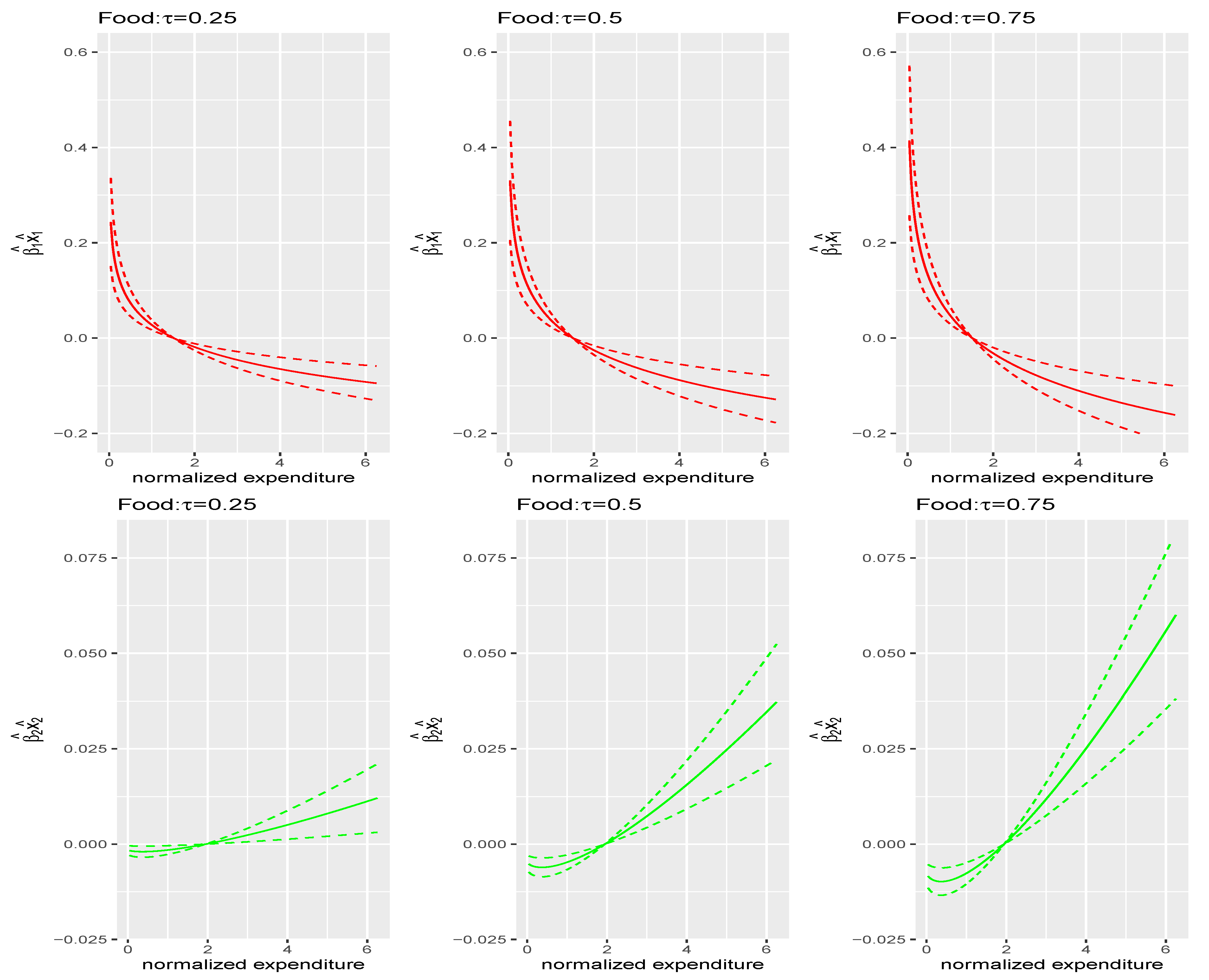
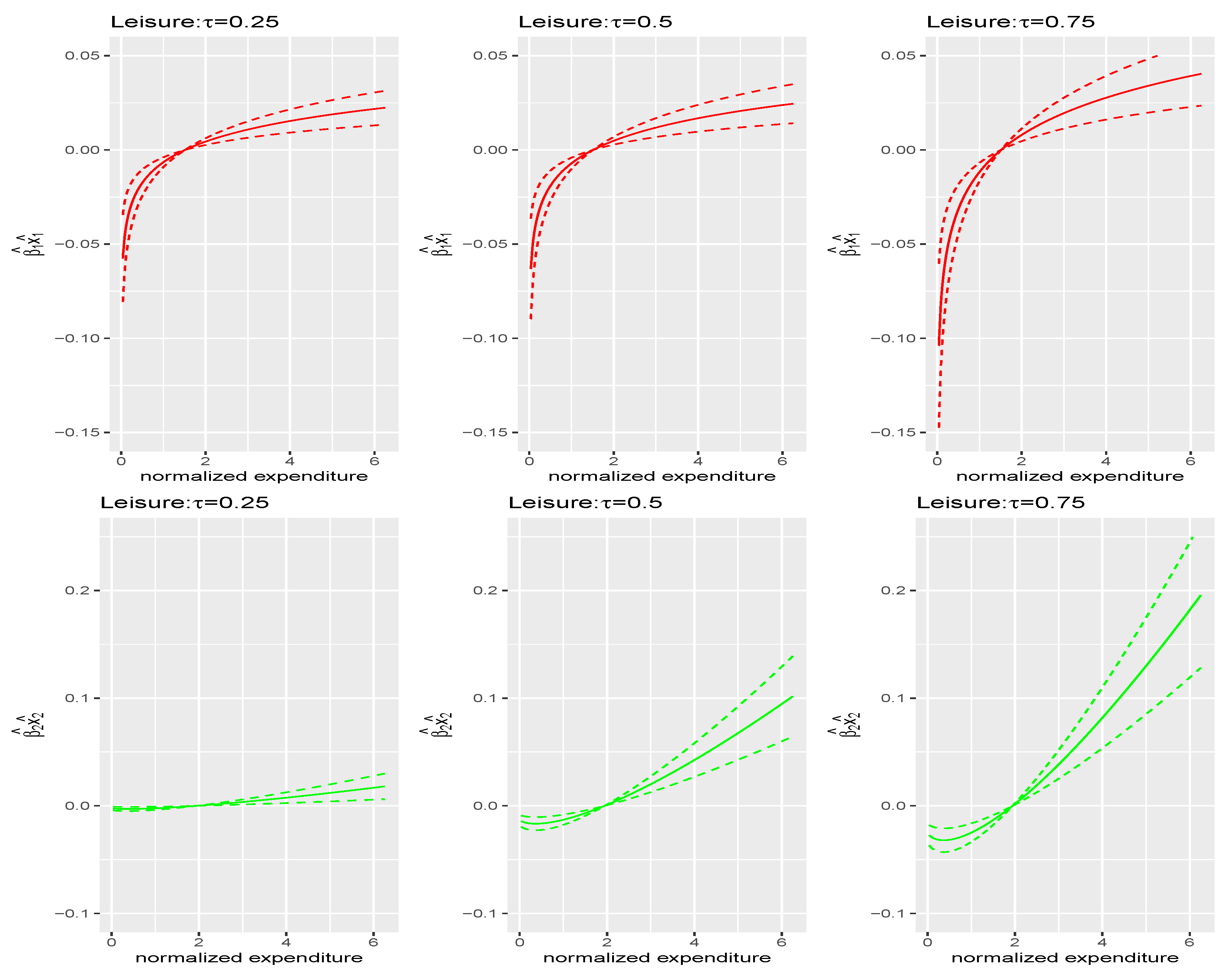
To help further interpret how the patterns of budget shares are related to these unobservable motives, we show how the budget share of a particular commodity varies over the total expenditure in Figure 2, Figure 3 and Figure 4. We estimate the contribution of each motive to the budget share at different quantiles $\tau \in \{0.25,0.5,0.75\}$. It is interesting to see how the motive to consume a particular commodity as necessity or luxury contributes to its budget share at different levels of total expenditure.

For instance, Figure 2 shows that, as total expenditure increases, the contribution of the first motive, $x_1$ (necessity), to food budget share decreases at all $\tau$, while the second motive, $x_2$ (luxuries), increases, as well documented in the literature. This implies that as total expenditure increases, the motive to consume food as a necessary good decreases, while the motive to consume food as a luxury good increases. The pattern in Figure 3, which is very different from food, reflects that individuals consume housing more as necessity but less as luxury, as their total expenditure increases. The motives to consume food and housing as necessity or luxuries play opposite roles in the budget share as total expenditure changes. However, as shown in Figure 4, both motives to consume leisure increase as total expenditure increases as well. Another interesting point is that the magnitudes of those estimated factors or motives are different across different quantiles of the conditional distribution of budget shares in all three commodities.

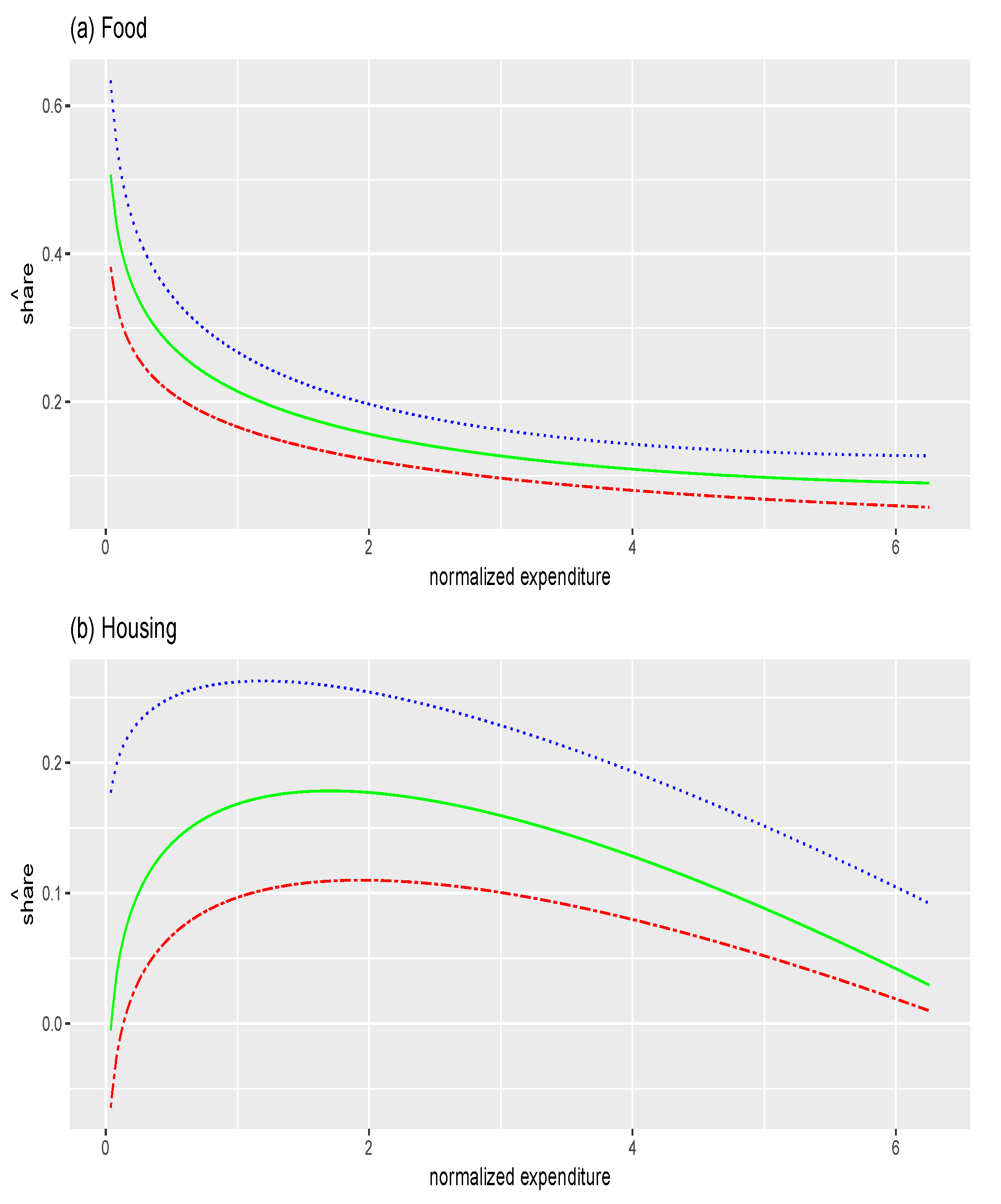
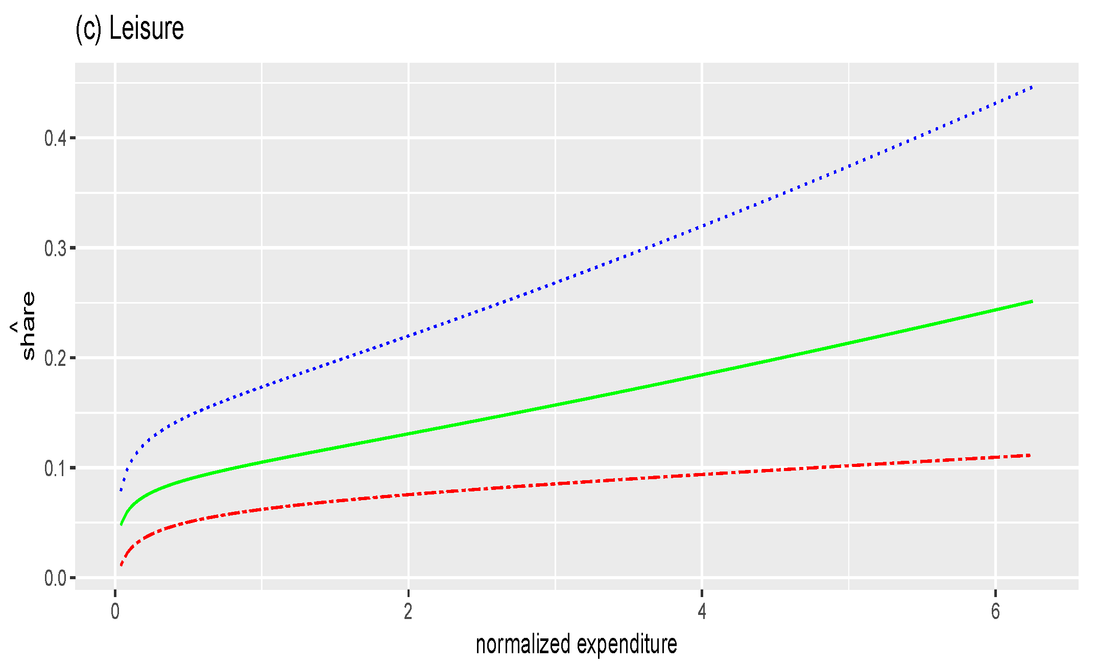
Figure 2, Figure 3 and Figure 4 suggest that the motive of consumption as necessity or luxury plays different roles over the level of total expenditure. The overall effects of total expenditure on budget shares are presented in Figure 5. The estimated budget shares are calculated by adding all three factors together. Figure 5a shows that the budget share of food decreases as total expenditure increases, which is classically referred to as Engel’s law. In Figure 5b we see a concave shape curve, that is, the budget share of housing increases for low expenditures, but decreases as total expenditure increases. In addition, individuals always raise the budget share of leisure as they consume more, as shown in Figure 5c. Finally, in housing and leisure, the shapes of the curves vary over different quantiles $\tau$. There is evidence of substantial asymmetry for the expenditure on housing and leisure, while there is less evidence of asymmetry for food share. For instance, we observe a shift toward leisure at the upper quantile of the leisure share. Thus, the conditional quantile approach would be a useful tool to capture asymmetric patterns of Engel curves across quantiles of budget share.

7. Conclusions

We study estimation and inference for linear quantile regression (QR) models with generated regressors (GR). We propose a QR-GR two-step estimator for the parameters of interest and an estimator for the corresponding asymptotic variance-covariance matrix. We establish the asymptotic properties of the estimators. Monte Carlo simulation and estimation of the Engel curves using data from the UK Family Expenditure Survey confirm that taking into account the GR problem in the QR framework is essential for correct inference. Furthermore, the empirical application shows strong heterogeneity of the Engel curves over different quantiles of the conditional distribution of budget shares in most commodities.

References

- Ackerberg, Daniel, Xiaohong Chen, Jinyong Hahn, and Zhipeng Liao. 2014. Asymptotic efficiency of semiparametric two-step gmm. Review of Economic Studies 288: 919–43. [Google Scholar] [CrossRef] [Green Version]
- Arellano, Manuel, and Stéphane Bonhomme. 2018. Sample selection in quantile regression: A survey. In Handbook of Quantile Regression. Edited by Koenker Roger, Victor Chernozhukov, Xuming He and Limin Peng. Boca Raton: CRC/Chapman-Hall. [Google Scholar]
- Bai, Jushan, and Serena Ng. 2002. Determining the number of factors in approximate factor models. Econometrica 70: 191–221. [Google Scholar] [CrossRef] [Green Version]
- Barigozzi, Matteo, and Alessio Moneta. 2016. Identifying the independent sources of consumption variation. Journal of Applied Econometrics 31: 420–49. [Google Scholar] [CrossRef] [Green Version]
- Barro, Robert J. 1977. Unanticipated money growth and unemployment in the united states. The American Economic Review 67: 101–15. [Google Scholar]
- Barro, Robert J. 1978. Unanticipated money, output, and the price level in the united states. Journal of Political Economy 86: 549–80. [Google Scholar] [CrossRef]
- Blundell, Richard, Xiaohong Chen, and Dennis Kristensen. 2007. Semi-nonparametric iv estimation of shape-invariant engel curves. Econometrica 75: 1613–69. [Google Scholar] [CrossRef] [Green Version]
- Buchinsky, Moshe, and Jinyong Hahn. 1998. An alternative estimator for the censored quantile regression model. Econometrica 66: 653–71. [Google Scholar] [CrossRef]
- Chai, Andreas, and Alessio Moneta. 2010. Retrospectives: Engel curves. Journal of Economic Perspectives 24: 225–40. [Google Scholar] [CrossRef] [Green Version]
- Chen, Liang, Juan Jose Dolado, and Jesus Gonzalo. 2015. Quantile factor models. arXiv arXiv:1911.02173. [Google Scholar]
- Chernozhukov, Victor, Ivan Fernandez-Val, and A. E. Kowalski. 2015. Quantile regression with censoring and endogeneity. Journal of Econometrics 186: 201–21. [Google Scholar] [CrossRef]
- Chernozhukov, Victor, and Christian Hansen. 2005. An iv model of quantile treatment effects. Econometrica 73: 245–61. [Google Scholar] [CrossRef] [Green Version]
- Chernozhukov, Victor, and Christian Hansen. 2006. Instrumental quantile regression inference for structural and treatment effects models. Journal of Econometrics 132: 491–525. [Google Scholar] [CrossRef]
- Engel, Ernst. 1857. Die productions-und consumtionsverhältnisse des königreichs sachsen. Zeitschrift des Statistischen Bureaus des Königlich Sächsischen Ministeriums des Innern 8: 1–54. [Google Scholar]
- Engle, Robert F. 1982. Autoregressive conditional heteroscedasticity with estimates of the variance of united kingdom inflation. Econometrica 50: 987–1007. [Google Scholar] [CrossRef]
- Firpo, Sergio, Antonio F. Galvao, and Suyong Song. 2017. Measurement errors in quantile regression models. Journal of Econometrics 198: 146–64. [Google Scholar] [CrossRef]
- Hahn, Jinyong, and Geert Rider. 2013. Asymptotic variance of semiparametric estimators with generated regressors. Econometrica 81: 315–40. [Google Scholar]
- Hendricks, Wallace, and Roger Koenker. 1991. Hierarchical spline models for conditional quantiles and the demand for electricity. Journal of the American Statistical Association 87: 58–68. [Google Scholar] [CrossRef]
- Koenker, Roger, and Gilbert Bassett. 1978. Regression quantiles. Econometrica 46: 33–50. [Google Scholar] [CrossRef]
- Koenker, Roger, and Gilbert Bassett. 1982a. Robust tests for heteroscedasticity based on regression quantiles. Econometrica 50: 43–61. [Google Scholar] [CrossRef] [Green Version]
- Koenker, Roger, and Gilbert Bassett. 1982b. Tests of linear hypotheses and l1 estimation. Econometrica 50: 1577–84. [Google Scholar] [CrossRef]
- Koenker, Roger, and José A. F. Machado. 1999. Goodness of fit and related inference processes for quantile regression. Journal of the American Statistical Association 94: 1296–310. [Google Scholar] [CrossRef]
- Lee, Sokbae. 2007. Endogeneity in quantile regression models: A control function approach. Journal of Econometrics 141: 1131–58. [Google Scholar] [CrossRef] [Green Version]
- Lewbel, Arthur. 1997. Consumer demand systems and household equivalence scales. Handbook of Applied Econometrics 2: 167–201. [Google Scholar]
- Lewbel, Arthur. 2008. Engel curves. The New Palgrave Dictionary of Economics 2: 1–4. [Google Scholar]
- Ma, Lingjie, and Roger Koenker. 2006. Quantile regression methods for recursive structural equation models. Journal of Econometrics 134: 471–506. [Google Scholar] [CrossRef] [Green Version]
- Mammen, Enno, Christoph Rothe, and Melanie Schienle. 2012. Nonparametric regression with nonparametrically generated covariates. Annals of Statistics 40: 1132–70. [Google Scholar] [CrossRef]
- Murphy, Kevin M., and Robert H. Topel. 2002. Estimation and inference in two-step econometric models. Journal of Business & Economic Statistics 20: 88–97. [Google Scholar]
- Pagan, Adrian. 1984. Econometric issues in the analysis of regressions with generated regressors. International Economic Review 25: 221–47. [Google Scholar] [CrossRef]
- Powell, James L. 1991. Estimation of monotonic regression models under quantile regressions. In Nonparametric and Semiparametric Models in Econometrics. Edited by William A. Barnett, James Powell and George E. Tauchen. Cambridge: Cambridge University Press. [Google Scholar]
- Wang, Huixia Judy, Leonard A. Stefanski, and Zhongyi Zhu. 2012. Corrected-loss estimation for quantile regression with covariate measurement errors. Biometrika 99: 405–21. [Google Scholar] [CrossRef] [Green Version]
- Wei, Ying, and Raymond J. Carroll. 2009. Quantile regression with measurement error. Journal of the American Statistical Association 104: 1129–43. [Google Scholar] [CrossRef] [PubMed] [Green Version]
- Working, Holbrook. 1943. Statistical laws of family expenditure. Journal of the American Statistical Association 38: 43–56. [Google Scholar] [CrossRef]
- Xiao, Zhijie, and Roger Koenker. 2009. Conditional quantile estimation for generalized autoregressive conditional heteroscedasticity models. Journal of the American Statistical Association 104: 1696–712. [Google Scholar] [CrossRef]
Figure 1.
Coefficient estimates of motives 1 and 2 and their 95% confidence intervals. (a) food budget share; (b) housing budget share; (c) leisure budget share. Upper row: coefficient estimates of factor 1; lower row: coefficient estimates of factor 2. Black line: OLS coefficient estimate; solid line: quantile regression (QR) coefficient estimate; dotted line: 95% confidence intervals obtained by conventional estimation; dashed line: 95% confidence intervals obtained by our proposed estimation.
Figure 2.
Contributions of motive 1 (upper row) and motive 2 (lower row) to food budget share; dotted lines are the corresponding confidence intervals.
Figure 3.
Contributions of motive 1 (upper row) and motive 2 (lower row) to housing budget share; dotted lines are the corresponding confidence intervals.
Figure 4.
Contributions of motive 1 (upper row) and motive 2 (lower row) to leisure budget share; dotted lines are the corresponding confidence intervals.
Figure 5.
Fitted values of budget share where . (a) food; (b) housing; (c) leisure. Red two dashed line: corresponding coefficients estimated at ; green solid line: corresponding coefficients estimated at ; blue dotted line: corresponding coefficients estimated at .