
An Empirical Model of Medicare Costs: The Role of Health Insurance, Employment, and Delays in Medicare Enrollment


1
ARC Centre of Excellence in Population Ageing Research (CEPAR), University of New South Wales, Sydney, NSW 2052, Australia
2
Department of Economics, Stony Brook University, Stony Brook, NY 11794-4384, USA
*
Author to whom correspondence should be addressed.
Econometrics 2021, 9(2), 25; https://0-doi-org.brum.beds.ac.uk/10.3390/econometrics9020025
Submission received: 22 February 2021
/
Revised: 22 May 2021
/
Accepted: 2 June 2021
/
Published: 8 June 2021
(This article belongs to the Special Issue Health Econometrics)
Abstract
:Medicare is one of the largest federal social insurance programs in the United States and the secondary payer for Medicare beneficiaries covered by employer-provided health insurance (EPHI). However, an increasing number of individuals are delaying their Medicare enrollment when they first become eligible at age 65. Using administrative data from the Medicare Current Beneficiary Survey (MCBS), this paper estimates the effects of EPHI, employment, and delays in Medicare enrollment on Medicare costs. Given the administrative nature of the data, we are able to disentangle and estimate the Medicare as secondary payer (MSP) effect and the work effects on Medicare costs, as well as to construct delay enrollment indicators. Using Heckman’s sample selection model, we estimate that MSP and being employed are associated with a lower probability of observing positive Medicare spending and a lower level of Medicare spending. This paper quantifies annual savings of $5.37 billion from MSP and being employed. Delays in Medicare enrollment generate additional annual savings of $10.17 billion. Owing to the links between employment, health insurance coverage, and Medicare costs presented in this research, our findings may be of interest to policy makers who should take into account the consequences of reforms on the Medicare system.
1. Introduction
Medicare, which had over 62.8 million beneficiaries as of 2020 and $799.4 billion in expenditures in 2019, is one of the largest federal social insurance programs in the United States.1 It is the secondary payer for Medicare beneficiaries aged 65 and older who are covered by employer-provided health insurance (EPHI) sponsored by firms with more than 20 employees. This so-called Medicare as Secondary Payer (MSP) provision was passed by the U.S. Congress in 1980, adding Section 1862(b) to Title XVIII of the Social Security Act, as a government cost-saving measure to make sure private insurers pay for the health care costs that they are responsible for. A sizable proportion of the aged population of the United States have dual health insurance coverage—from the Medicare system and from EPHI.2
The Medicare system has been studied in detail from many perspectives, but researchers have rarely discussed the link between Medicare costs, delays in Medicare enrollment, and delayed Medicare enrollment penalties, as well as their link with EPHI, which, in this paper, is defined as a group health plan through current employment or through a spouse’s current employment. These links are of great importance after more than two decades of increased labor force participation of older Americans, and the increasing pressure to reform the Social Security System, which is likely to result in further increases in the employment level and the number of older Americans with EPHI.3
A cross-tabulation using the Medicare Current Beneficiary Survey (MCBS) points to a large and significant difference in average Medicare spending among Medicare beneficiaries with and without EPHI coverage. We calculate that annual average Medicare spending per enrollee among beneficiaries with EPHI coverage (where Medicare is the secondary payer) totaled $4156 over the 1999–2010 period. In contrast, annual average Medicare spending among beneficiaries without EPHI coverage (where Medicare is the primary payer) was $7096.4
One empirical challenge in estimating the effects of EPHI on Medicare costs is to disentangle the MSP effect from the work effect. Given that EPHI is defined as a group health plan through current employment or through a spouse’s current employment, an individual can be covered by EPHI without being employed (the MSP effect), or by being employed without EPHI coverage (the work effect), or by being employed and covered by EPHI (the compound effect). The MCBS, which covers those mutually exclusive sub-samples, allows us to identify those effects separately. To our knowledge, we are the first to identify and estimate the MSP and work effects on Medicare costs. We also calculate the Medicare cost savings resulting from the MSP provision using administrative data, and Medicare cost savings from individuals working as an effect independent of insurance status.
While a majority of Americans enroll in Medicare when they first become eligible at age 65, more individuals are delaying their Medicare enrollment. Using the MCBS over the 1999–2010 period (see Figure 1), we calculate that the proportion of individuals who delay Medicare Part B (outpatient services) has increased considerably for male enrollees, from 4.56 percent in 1999 to 8.38 percent in 2010 (2.28 percent in 1999 to 3.96 percent in 2010 for female enrollees). Over the same period, a small proportion of individuals delayed Part A (inpatient services).5 A key aspect of the Medicare enrollment choice is that the government imposes penalties on those who delay Medicare enrollment more than 12 months after the end of the seven-month initial enrollment period (IEP), which ends when the individual reaches age 65 and three months, while not covered by EPHI. The rationale for these penalties has not been carefully discussed in the literature or by the government, but it is easy to conjecture that it is linked to the desire to prevent individuals from generating higher Medicare costs (once they enroll). Presumably, this strategy guards against adverse selection from individuals waiting until a negative health shock to decide on a plan.6
The decision of individuals to delay their access to Medicare has not been studied in much detail, and it has been rarely modeled by economists. In empirically estimating the effect of delay behaviors on Medicare costs one is faced with challenges linked to identifying those current (past) delayers who delay (delayed) their Medicare enrollment. Specifically, current delayers are Medicare beneficiaries with only Part A (Part B) coverage, therefore delaying Part B (Part A). Past delayers are Medicare beneficiaries who have delayed both Parts A and B, which requires a retrospective assessment. In both cases, we consider someone as a delayer if they have reached age 66 without being enrolled in either or both parts of Medicare.
One important contribution of this paper lies in our analysis which uses administrative data from the MCBS to estimate the effects of delays in Medicare enrollment on Medicare costs, by constructing delay enrollment indicators, and to calculate the Medicare cost savings from individuals’ delay behaviors. One key advantage of the MCBS is that it contains individual-level Medicare enrollment dates, Medicare status, and Medicare entitlement information, all of which allow the delayers to be identified.
Our empirical findings indicate that MSP and being employed are associated with a lower probability of observing positive Medicare spending, and a lower level of Medicare spending. Specifically, MSP significantly lowers the probability of observing positive Medicare costs by 5.5 percent and the level of Medicare spending by 7.6 percent. Being employed is associated with decreased probability of observing positive Medicare costs by 7.5 percent and decreased level of Medicare spending by 10.8. Our sensitivity analysis outlined in Section 4 suggests that our results using our preferred specification are likely to be on the conservative side. The effect on Medicare costs of currently delaying Medicare Part A or Part B is comparatively small.
Our empirical results allow us to quantify the savings to the Medicare system from MSP and being employed, from 1999–2010, which amount to annual savings of $5.37 billion. The $5.37 billion annual saving represents savings of 1.12 percent of the total Medicare Personal Health Care in 2010.7 Most of the changes in savings over time are linked to the increase in the number of people aged 65 and over, and the evolution of labor force participation of older Americans. Delays in Medicare enrollment generate additional annual savings of $10.17 billion, mostly coming from our retrospective calculations of delayed enrollment. The $10.17 billion annual saving represents savings of 2.12 percent of the total Medicare Personal Health Care in 2010. Overall, the savings we present in this research represent on average around 4 percent of the total Medicare Personal Health Care in the period of analysis, with a range between 3.25 percent and 5.04 percent, depending on the year analyzed. Interestingly, our analysis brings positive news to the discussion of the Medicare system, providing, at least from these sources, cost savings instead of ever growing costs.8
Our findings relate to several literatures. The most relevant analyzes Medicare costs, and in particular the relationship between Medicare supplemental insurance and Medicare costs, and finds that Medigap insurance is associated with increased Medicare costs per enrollee by between 10 percent (Ettner 1997) and 22.2 percent (Cabral and Mahoney 2019). Both studies focus on the additional coverage which maintained Medicare as primary payer. Khandker and McCormack (1999), using MCBS, find that Medicare enrollees covered by Medigap and health insurance coverage through employment incur higher Medicare spending. Hurd and McGarry (1997), using the Asset and Health Dynamics Survey, find that those with private health insurance (through a former employer or purchased in the market) additional to Medicare tend to use services more. Notice, however, that Khandker and McCormack (1999) do not separate retiree health insurance through former employer (Medicare works as primary payer) from EPHI in their estimation, and Hurd and McGarry (1997) do not use indicators of EPHI coverage due to data limitations. Thanks to the richness of the MCBS, our focus is on the type of coverage (EPHI) which makes Medicare a secondary payer, and our estimation suggests that EPHI is associated with a lower probability of observing positive Medicare spending, and a lower level of Medicare spending.9
While the savings from MSP are discussed in Glied and Stabile (2001) and Goda et al. (2007), they use older, noisier, and mostly aggregate data sources. Glied and Stabile (2001), who focus on the period following the implementation of the law in the mid- to late 1980s, find that MSP only generated 25–33 percent of its intended savings to the Medicare system because of lack of compliance among employers, a problem that is unlikely to be of much relevance during our period of analysis. Goda et al. (2007) do not seem to separate the work effect from the EPHI effect, and more importantly they do not link the MSP provision with the delays in enrollment, a phenomenon hard to reconcile without understanding the role played by EPHI. Goda et al. (2011) focus on the implicit tax imposed on employers and employees due to the MSP provision. They find that eliminating the MSP provision would remove a work disincentive from working beyond 65, but, given that their calculations are set up in a non-utility based model, it is unclear to us whether this removal would actually result in a welfare improving situation for those affected by the MSP provision.
Using a very different definition, Sloan et al. (2012) is the only other paper that studies delays in the Medicare system. However, Sloan et al. (2012) do not account for delay in enrollment, just delay in first usage of Part B services among enrollees. Additionally, Sloan et al. (2012) do not attempt to study the consequences of delayed usage for the financial status of the Medicare system.
The remainder of the paper is organized as follows. Section 2 describes the MCBS data and how we empirically identify Medicare delayers. Section 3 provides the empirical analysis of the determinants of Medicare costs and our main empirical findings. Section 4 provides the sensitivity analysis of our results. Section 5 shows the calculation of Medicare savings. Section 6 presents our conclusions.
2. Data and Medicare Delayers
2.1. MCBS Data
We use the MCBS, a nationally representative dataset set up by the Centers for Medicare & Medicaid Services (CMS), which has two modules: MCBS Access to Care and MCBS Cost and Use. MCBS produces data for both cross-sectional and longitudinal analysis. For the purpose of this research, we use the Cost and Use series.10 The Cost and Use data provide complete expenditure and source of payment data on all health care services, including those not covered by Medicare. They also provide information on individual-level premiums, health insurance coverage and usage, Medicare entitlement information, health status and functioning, date of death, Medicare status, and Medicare claims for survey participants.
In this research, we only focus on aged Medicare beneficiaries, who accounted for 83.1 (86.7) percent of Medicare beneficiaries in 2010 (2020).11 Medicare entitlement start and end dates help identify when an individual enrolled in Medicare and how long that individual stays in Medicare. A great advantage of the Cost and Use files is that the data match survey-reported events with true Medicare claims, adjusting for under-reporting of the use of health care services by survey respondents and correcting any recall mistakes in the survey expenditure data. Therefore, MCBS is considered the best possible source of information on Medicare costs. Details of our sample selection criteria and descriptive statistics are in Appendix A.1.
Table 1 presents unconditional evidence that both working and health insurance are correlated with Medicare costs. We summarize Medicare costs, total health expenditure, as well as out-of-pocket (OOP) expenditure, by working status, as well as EPHI status, also conditional on a particular age range and health status. The full estimation sample is divided into four subgroups: (working, no EPHI), (working, EPHI), (not working, no EPHI), and (not working, EPHI). Four aspects require attention. First, both working and EPHI lower the average Medicare costs. For individuals aged 65–69, and in good health, the weighted average Medicare cost is $1404 for workers with EPHI and $3245 for non-workers with EPHI, a difference that can be understood as the effect of working on Medicare costs, controlling for EPHI, as well as age and health status. If we try to infer the effect of EPHI on Medicare costs, we compare across columns two by two, and we can see that the effect is much larger among workers, and especially larger among those in bad health.12 Second, among workers, those covered by EPHI generate fewer Medicare costs, but they have slightly higher total health expenditure, in addition to OOP expenditure regardless of health status. This suggests that workers covered by EPHI are not necessarily low medical cost generators. Rather, it is the result of Medicare appearing only as the secondary payer. We will argue that this is evidence of exogeneity of the EPHI variable in our econometric specifications. Third, non-workers tend to generate higher Medicare and total health expenditure, especially when in bad health. Finally, OOP expenditure is very similar for workers and non-workers, as well as for those with or without EPHI; the main difference appears across health status categories. This finding suggests that individuals seem to be making their decisions in order to minimize OOP costs, navigating the complexity of the system, and its interactions, fairly well. Notice that all dollar values shown throughout the paper are inflation-adjusted to 2009 using the medical care CPI.
2.2. Empirically Identifying Medicare Delayers
As discussed in the Introduction, a significant proportion of Americans delay their access to Medicare, particularly Part B. It is important to discuss the empirical challenges linked to identifying, in the MCBS, those individuals who are delaying (or have delayed) their access to Medicare. Notice that, while other definitions are possible (given the way the government defines IEP), we consider that someone has delayed their access to Medicare if they have reached age 66 without being enrolled in both parts (Part A and Part B) or either part of Medicare.
Our efforts focus on three aspects of the measurement of delay behavior. First, current delayers are Medicare beneficiaries who have only Part A coverage and are delaying Part B, as well as those who have only Part B coverage and are delaying Part A. By definition we can only observe current delayers if they are actually already enrolled in one part of the program and delaying another. This also means that those who are completely delaying their entrance into Medicare will not be observed in the periods in which they are doing it, so a retrospective perspective will be needed. Second, past delayers refer to Medicare beneficiaries who have delayed both parts of Medicare. Once an individual is enrolled and observed in the data, we can retrospectively assess whether they were a previous delayer, and pin down during which period, by comparing their initial enrollment date with their age at the time. However, we will not always be able to exactly observe what Medicare part the individual was delaying, unless we can use their current enrollment status to impute their likely delay behavior. For example, if someone is currently enrolled in both Part A and Part B of the system, and we observe that they enrolled in the system at age 67—so they delayed when they were 65 and 66—, we will assume that they delayed both parts during that period. On the other hand, if they are currently enrolled only in Part A, and they enrolled in the IEP, we will assume that they delayed only Part B in those years. We are essentially ruling out the possibility of switching Medicare coverage (as well as the possibility of dropping Medicare coverage), since we cannot precisely observe the coverage before the person appears in the MCBS. This retrospective calculation is quite tedious and requires us to look back at the data year by year, taking a retrospective perspective back to 1999. Third, delaying (delayed) access to Medicare could have consequences for the Medicare system if we believe individuals’ lack of access to this program could have delayed certain treatments or worsened a particular health condition. This means that we need to analyze whether individuals’ current (previous) Medicare enrollment status has a differential effect on current costs to the system. More specifically, we are interested in the effects of current delayers and past delayers on current Medicare costs. The richness of the MCBS allows the identification of delayers, as well as the construction of delay dummies.
3. Medicare Costs: An Empirical Analysis
3.1. Empirical Challenges and Model Specifications
The estimation of Medicare costs brings two important challenges which need to be considered to consistently estimate the role of work and EPHI. The first is that there is a potential selection problem, given that nearly 19 percent of observations in our sample have Medicare costs equal to zero. These true zeros either come from some individuals not generating any expenditure in any given year, or from a situation in which they generate health expenditure but health coverage other than Medicare paid for them.13 Notice that the true zero Medicare cost is not a direct choice of individuals; in other words, individuals cannot choose to have zero Medicare costs, but it can be the product of decisions related to work and health insurance coverage. If individuals self-select into certain jobs with certain EPHI coverage, then Medicare becomes a secondary payer. Under the regulations of multiple payers, the government might end up paying nothing for them in a given year. It could be that the people who have zero Medicare costs are not a random sample of the population; there could be a potential correlation between the choices that lead to zero Medicare costs and the level of the costs. Thus, we need to consider the potential selection problem.
The second issue is the possible endogeneity of the and indicators: workers are different from non-workers, and workers are not randomly selected into working, nor do they randomly decide to keep working after age 65. Given that individual characteristics affect individuals’ labor decisions after 65, if some of these characteristics are unobserved (e.g., income shocks or health insurance benefit shocks), and are correlated with the indicator, then the estimated coefficient ( in Equation (2)) could be biased. On the other hand, the choice of work in a job covered by EPHI might be correlated with unobservables linked with, for example, lower health care expenditure.
In order to estimate how a number of observable characteristics, including insurance plans, affect medical expenditure, several models have been proposed and used in the literature. Ordinary least squares (OLS) estimation is simple and easy to interpret, but can be problematic to use when the data contain a relatively large number of zeros. The two-part model (TPM) (Duan et al. 1983), presented by Ettner (1997) and Khandker and McCormack (1999), has all the advantages of the OLS while still acknowledging that the zeros are not the product of choice, but rather the absence of expenditure; however, there is also no correction for the possible correlation between the probability of having zero Medicare costs and the level of the costs. Panel data specifications and instrumental variable (IV) specifications help to directly address the possible endogeneity concerns. The panel component of the MCBS (four years, at most) allows us to deal with the endogeneity problem by including individual fixed effects to control for any fixed, time-invariant, individual unobserved factor. For IV estimation, finding robust and exogenous exclusion restrictions is crucial. These exclusion restrictions should be correlated with individuals’ working decision, captured in our case by the dummy, and should not be correlated with the error term in the Medicare cost equation. This requirements are rather challenging in the MCBS, in which, unlike traditional household surveys, we do not have access to a wide range of family-level characteristics that could, for example, be considered as natural exclusion restrictions in an IV setting. Still, we have experimented with IV estimation and provide detailed results when presenting the sensitivity analysis to our main findings.
Under Heckman’s sample selection model (Heckman 1979), the censoring function and the uncensored expenditure function can have different coefficients and correlated unobservables are also possible across the two processes. It is also our preferred model specification because the inverse Mills ratio is statistically significant. In Heckman’s model, there are two separate equations: first, an equation that estimates the probability of having positive health expenditure , and second, a specification that estimates the level of expenditures, conditional on those being positive . Usually, the first equation will use a probit specification to estimate the dichotomous event of having zero or positive expenses, and the second equation is a linear model, on the log scale for positive expenditure.
We investigate the effect of health insurance coverage and employment on individuals’ Medicare costs, total health expenditure, and OOP expenditure by running the specifications below. Equation (1) is used in the first stage of Heckman’s sample selection model, and Equation (2) is used in the second stage, where is a dummy equal to one when medical expenditure, , is greater than zero; and is a vector of regressors, including the dummy, the dummy, the dummy, health controls, demographic controls, and dummies.
In this specification, dummies are used as an exclusion restriction, which only appears in Equation (1) to add non-parametric identification. That equation is originally parametrically identified through the non-linearity created by the probit assumptions. We construct dummy variables indicating the effects of delayed retirement credits (DRC) and/or full retirement age (FRA) for each respondent in the sample according to their birth year, the DRC, and the FRA rules. Cohorts born in 1925 and 1937 are only affected by DRC, and is a dummy indicating cohorts born in 1925 and 1926 with 3.5 percent DRC. Cohorts born in 1938 or later are affected by both DRC and a FRA. is a dummy indicating a cohort born in 1938 with 6.5 percent DRC and a FRA of 65 and two months. Similarly, represents cohorts born in 1939 with 7 percent DRC and a FRA of 65 and four months. Owing to data limitations, the youngest cohort we are able to observe in the MCBS is individuals born in 1945, with DRC of 8 percent and a FRA of 66.
Unlike the IV specification, there are no standard tests of the robustness and exogeneity of the exclusion restrictions assumed in Heckman’s sample selection model, since that model is already identified and we are just adding non-parametric identification to it. As discussed in Vella (1998), it is customary to add this non-parametric identification, but there is some contention as to whether these exclusion restrictions should even be used. In any case, we will see in the results in Appendix A Table A3 that the DRC/FRA indicators are positive and significant in the probit equation, and if we estimate a model without those exclusion restrictions, that is, a “just parametrically identified” sample selection corrected model, our results are quite similar to those reported. As also discussed in Vella (1998), if the independent variables we use in the probit specification have a large range (as we believe they do), the concerns related to the “just parametrically identified model” are ameliorated, since more tail behavior is expected in the inverse Mills ratio. We obtain the probit estimate from Equation (1) using the full estimation sample and then obtain the estimated inverse Mills ratio .
In Equation (2), is one of the outcomes of interest (e.g., Medicare costs, total health expenditure, and OOP expenditure) for individual i in year t, while the dependent variable is the natural logarithm of one of the outcomes of interest for individual i in year t. The explanatory variables in Equation (2) are the same as in Equation (1); the only difference is that the dummies only appear in Equation (1). is a dummy variable that represents those who are working. , refers to individual i who is covered by EPHI at time t regardless of their working condition, and captures the effect of MSP. Recall from Section 1 that EPHI is defined as a group health plan through current employment or a spouse’s current employment.14 We also add an interaction term, , between work and the EPHI indicator, to show the differential effects more clearly between insurance and work. These two measures are correlated, but there are individuals who work without EPHI, as well as individuals who have EPHI and do not work. is a list of health controls.15 is a list of demographic controls—for example, gender, race, individual-level income, marital status, education, census regions, age, age squared, and number of kids. Finally, is the unobservable component. The base group in the estimation includes those who are not working, those who are not covered by EPHI, those whose census region is the north-east, those whose annual household income is less than $10,000 (in 2009 dollars), those who are married, those who are white, those who have a high school degree, and those whose health status is excellent or very good.
3.2. The Effect of Working and Medicare Secondary Payer on Medicare Costs
Table 2 shows the marginal effects from the first stage of Heckman’s sample selection model for Medicare costs (column (1)), total health expenditure (column (2)), and OOP expenditure (column (3)), which estimates a probit specification. Table 3 shows the results of the second stage of Heckman’s sample selection model. The inverse Mills ratio is significant and negative across the board, indicating that the sample selection model is appropriate, and the error terms in the selection and primary equations are negatively correlated.
From Table 2, we can see that the dummy significantly lowers the probability of observing positive Medicare costs. Now, conditional on having positive Medicare costs, as shown in Table 3, workers generate 7.6 percent lower Medicare costs compared with non-workers, after conditioning for health insurance coverage. Since we also control for health indicators, as well as other demographic measures and observables, the possible explanation for workers generating fewer costs mainly comes down to opportunity costs, and, therefore, unobservables. For example, workers have less time and less availability to go to Medicare services compared with non-workers, so workers tend to use Medicare less, resulting in a lower Medicare cost per person, on average. Interestingly, the dummy is also negative and significantly correlated with total health expenditure (but not OOP expenditure) in Table 3, suggesting a possible concern for the endogeneity of this measure, since workers might be generating systematically lower health costs. The “just parametrically identified” sample selection corrected estimates of the variable, that is, those resulting from estimating the two-step Heckman model without exclusion restrictions, are quite similar to those reported. In Table 2, the coefficient changes from an estimated reduction in the probability of observing positive Medicare costs of 5.5 percent to 5.3 percent. On the other hand, in Table 3, the reduction in the level of Medicare costs goes from the reported 7.6 percent to 8.8 percent. Overall, the specification that adds non-parametric identification is more conservative in terms of the overall effects of the dummy.
Given the definitions of the variables discussed in the previous subsection, Medicare is the secondary payer only when the individual is covered through their current employer, or the current employer of a spouse. This is captured by the variable , which significantly reduces the probability of observing positive Medicare costs (Table 2), and also significantly reduces Medicare costs, conditional on them being positive (Table 3). On average, individuals with MSP generate 10.8 percent fewer Medicare costs compared to individuals with Medicare as primary payer. Notice that, in this case, the indicator affects total health expenditure and OOP expenditure positively (although the coefficients are small and not significant), likely indicating that, for this variable, the endogeneity concerns are minor, since it does not seem that those covered by EPHI are the lower cost-generating individuals (this is in line with the well-established literature which finds that, if anything, those with additional insurance coverage would generate higher expenditure to the Medicare system; see Khandker and McCormack (1999), for example). For the “just identified” specification, the negative effect in Table 3 goes up to 13 percent.
Table 3 also shows the negative effect on Medicare costs of the interaction term , indicating that those who work and have EPHI generate nearly 28.1 percent less cost to the Medicare system (31.7 percent in the “just parametrically identified” specification), compared to those who do not work and do not have EPHI. As with the indicator, endogeneity concerns are not of great importance with the indicator, given its either positive or non-significant effect on the other health expenditure measures.
3.3. Delayed Enrollment and Medicare Costs
Delaying (delayed) access to Medicare could have consequences for the Medicare system if individuals’ lack of access to the program delays certain treatments or worsens a particular health condition. In this section, we focus on the first and third aspects of the delay behavior that we raised in Section 2.2, namely estimation of the effect of a current delayer (currently delaying either Part A or Part B), and the effect of a past delayer (someone who has delayed before) on current Medicare costs. The use of retrospective information to compute the number of delayers in past years and the resulting savings will be discussed in Section 5.2.
Table 4 shows the second-stage estimation results using Heckman’s sample selection model (first-stage results are presented in Appendix A Table A5), after including delay enrollment dummies for current delayers in the Medicare costs regression, which essentially expands the set of regressors shown in Equations (1) and (2) to include the delay indicators. The left panel shows the results conditional on health status; the right panel contains the results without any health controls. We present the results without health controls because the effects of delays in Medicare enrollment on health care costs are connected to a deterioration of health, as a result of delaying access to care. Therefore, not controlling for health status could be a more appropriate specification to capture the effects of delays in Medicare enrollment. The Lambda in all cases are significant, indicating that the sample selection corrected specification is the appropriate one to use.
The results are quite striking. First, the key results we show in Table 3 are magnified in absolute terms, once we control for the respondents who are currently enrolled in only one part of Medicare, thus delaying the other part. The negative effect of working on Medicare cost increases by about a third, and the increases are even larger for the indicator and the variable. This likely means that the delay indicators are strongly correlated with the work and insurance indicators. Second, those who are currently delaying Part A (–A–), and, therefore, are currently enrolled in Part B, generate substantially lower Medicare costs, as well as lower total health expenditure and lower OOP expenditure. More surprising are the results which show that those who currently delay Part B (–B–) generate higher Medicare costs, other things equal, but lower total and OOP costs. This means that these individuals generate, comparatively, higher Part A costs, but are not necessarily high-cost-generating individuals, and they are certainly optimizers in terms of the OOP resources generated. The Part B result is better understood if we take a look at the first-stage results in Appendix A Table A5. There we can see that delaying Part B has a negative effect on the probability of observing positive Medicare costs, which means that Part B delayers are more likely to generate zero cost to the Medicare system. This effect is magnified among those who have EPHI and delay Part B (–B–). Notice that these effects are exactly reversed for Part A, which increases the probability of observing positive Medicare costs, but reduces the average costs conditional on a positive value. We will use these results in the next section to compute the savings to the system derived from the current delayers’ decision not to join one part of the program.
Table 5 focuses on the effect of past delayers who have delayed previously, captured by the – variable (which again expands the set of regressors presented in Equations (1) and (2), on the level of current Medicare costs with and without health controls, knowing that individuals, in their decision to delay, are responding to the structure of penalties set up by the government. The effect of past delayers on the probability of positive medical spending (the first-stage results) are presented in Appendix Table A6. The rationale for the penalties is likely due to the concern that those who delay, and who do not have alternative primary coverage, will end up generating higher costs once they enroll in Medicare. The results show that the – variable has a positive, but small and statistically insignificant, effect on Medicare costs, suggesting that individuals’ previous delay behavior (after they optimize their delay decisions accounting for penalties), regardless of whether we control for their health, has no statistical effect on Medicare costs. In Section 5, we will demonstrate how we can then use the information on delay behavior to calculate the savings for Medicare resulting from these delays.
4. Sensitivity Analysis of the Results
Table 6 presents the results of several specifications of the log of individuals’ Medicare costs as the dependent variable. Column (1) presents the results of the OLS regression, including the true zeros in the sample. The result is that the coefficients of interest are larger in absolute terms compared to our preferred specification, reflecting the likely bias of the estimated effect of the and variables, due to the fact that we are not separating the process that delivers the zero cost from the one that generates positive Medicare costs. From the data, we know that around 43 percent of those covered by EPHI have expenditure equal to zero. To account for this, the OLS coefficients have to be negative and large.16
Column (2) shows the results of fixed-effect (FE) specification of Medicare costs. Given that the FE estimator is able to remove the time-invariant unobserved individual components from the estimation, while allowing for correlation between the independent variables and the error term, this helps us address the possible endogeneity issues linked with the and indicators, without resorting to exclusion restrictions. Notice that the absolute value of the coefficients goes down considerably, but the Work and EPHI indicators are still negative and significant while the interaction term is very small and insignificant. These results suggest that, in the presence of bias due to endogeneity concerns, the FE estimator seems to work quite well.17 Column (3) presents the results from the second stage of the TPM. The first TPM stage is not presented because it is identical to the first stage of the Heckman’s sample selection model shown in Table 2. TPM does separate the zero and positive Medicare costs, but does not allow correlation between the error components of the specification of the probability of having positive Medicare costs, and the level of the costs. In this case, the size of the coefficient goes down further, while the is similar to that of the FE estimator. The interaction term is, again, negative and significant in this specification. Finally, column (4) shows the results from the second stage of Heckman’s sample selection model, which are the same as in Table 3. For the and estimates, this specification is the one that estimates the smallest (in absolute terms) effects, while the interaction term is smaller (in absolute terms) than for the OLS and TPM specifications, but larger than in the FE case.
Table 7 presents the results of several IV specifications of Medicare costs, allowing for the endogeneity of the indicator in the first four specifications presented in columns (1)–(4), and the endogeneity of the indicator in the last specification in column (5). The exclusion restrictions used is what differentiates the first four specifications: in all four cases, we use whether an individual is married as one of the exclusion restrictions (given its strong correlation with the work indicator); then, in turn, we use as the second exclusion restriction (to be able to test the exogeneity of the exclusion restriction by running an overidentification test) whether the individual acquired some college education (but do not have a BA degree) in column (1), the number of kids in column (2), the cohort indicator in column (3), and the cohort indicator in column (4). In column (5) of Table 7, we allow for the endogeneity of the indicator and use whether an individual is married and whether the individual acquired some college education as exclusion restrictions.
In Table 7, in order to assess the validity of the exclusion restrictions, we report the Kleibergen Paap rk Wald F-statistics that check the robustness of the exclusion restrictions in the first stage of the estimation procedure, and the Hansen J-Statistic to test the exogeneity of the restrictions. In addition, we show the results of the Hausman specification test that assesses the validity of the exogeneity assumption regarding the candidate endogenous variable. In all, the specifications in Table 7 shown the Hausman specification test cannot reject the null hypothesis that the candidate endogenous variable is exogenous, suggesting that OLS would provide consistent estimates of the studied effects. In all cases, the exclusion restrictions are deemed as robust, and only for the IV specifications in columns (2) and (4) are the exclusion restrictions not considered as exogenous at the 10% confidence level.
From Table 7, we can see that the and coefficients are quite similar for the first three specifications in columns (1)–(3), and the IV estimates of the indicator are much larger than their OLS counterparts (Table 6 column (1)), and, while significant, their standard errors are also much larger than the ones provided by OLS presented in Table 6 column (1). On the other hand, the estimates for the indicators are quite similar to those in the OLS estimation. The estimate for indicator in specification IV_4 in column (4) is smaller than for the first three specifications, and, in this case, it is not significant. For specification IV_5 presented in column (5), when we consider as the possibly endogenous regressor, the IV estimate for indicator actually turns positive but is highly insignificant, while the indicator is negative and significant. While many other IV specifications are possible, the ones presented above represent well the overall results, and a model selection exploration in the spirit of the Lasso technique would not provide a very different picture of what the IV technique can bring to the table.
Overall our sensitivity analysis suggests that choosing the Heckman’s sample selection specification minimizes the chance of observing upward bias in our coefficients (in absolute terms), while still controlling for sample selection, which seems warranted by the significance of the inverse Mills ratio. Since we use the results of column (4) in Table 6 in the calculations of the savings in the next section, it is important to notice that the Heckman’s results show the lower bound (in absolute terms) among all the estimates for the effects of the and indicators, and, for the effect of the interaction term, the Heckman’s sample selection specification is the second smallest (in absolute terms) after the FE.
5. Medicare Savings
Given the estimation results presented in Section 3, and using additional “back of the envelope” calculations regarding Medicare delay behaviors, we can quantify the annual Medicare savings resulting from the fact that: workers generate fewer costs to the Medicare system compared with non-workers; Medicare is a secondary payer for individuals covered by EPHI; and individuals delay enrollment into one or both parts of the program.
5.1. Medicare Savings from Work and the Medicare Secondary Payer Effect
The savings linked to work and the MSP effect come from two sources. First, work and EPHI decrease the probability of observing a positive Medicare cost in the first stage of our preferred Heckman’s sample selection specification. Second, for those with positive Medicare costs, we observe a decline in the level of Medicare spending due to work and EPHI.
Computing the total Medicare costs saved as a result of an individual working requires us to first calculate the average Medicare costs in a given year for those with positive costs. We then calculate the average annual number of individuals who are working and then compute the breakdown between those with zero Medicare costs and those with positive Medicare costs.
The top panel in Table 8 shows the weighted population of workers in selected years. In 2004, the number of workers is 4.48 million, whereas, in 2010, it is 5.61 million. Among the 4.48 million individuals in 2004, 63.54 percent have positive Medicare costs. Since the work effect, captured by the dummy in Section 3.2, reduces the probability of observing a positive Medicare cost by 6.79 percent (Appendix A.3 has details on how we compute these numbers), if the variable were to have zero effect on the probability of observing a positive Medicare cost, the breakdown between positive and zero Medicare costs would show that people with positive expenditure would be 68.17 percent instead of 63.54 percent. This means that is responsible for a reduction of 4.63 percentage points in the proportion of those who have positive Medicare costs. With this information, we are ready to compute the aggregate savings from the working effect.
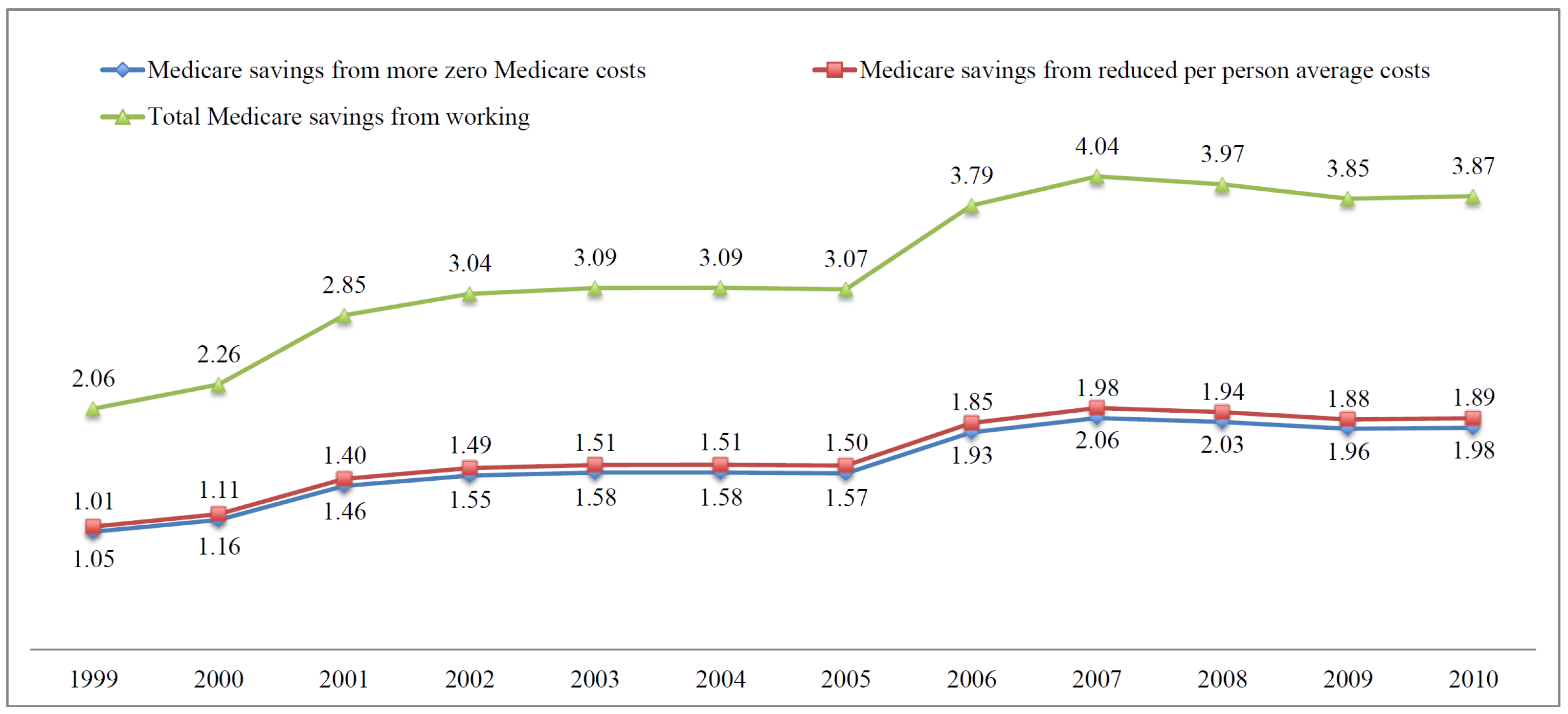
The 4.48 million workers in 2004 generate two sets of savings. First, given that we have more individuals with zero Medicare costs, the Medicare system saves $1.51 billion, which results from multiplying the average expenditure in 2004 of $7291.5 (rounded in the table) by the 4.48 million individuals, and by the 4.63 percent who change from the average to zero. Then, we have additional savings for those who have positive Medicare costs and see their average costs reduced due to the effect of working. Those savings are $1.58 billion (multiply 4.48 million by $7,291.5 per individual, by the coefficient of the indicator in Table 3, and by the 63.54 percent who have positive Medicare costs). These two effects add up to $3.09 billion in 2004. For 2010, savings are $3.87 billion. The average yearly savings amount during the 1999–2010 period is $3.25 billion, which represents savings of 0.68 percent of the total Medicare Personal Health Care expenditure in 2010.
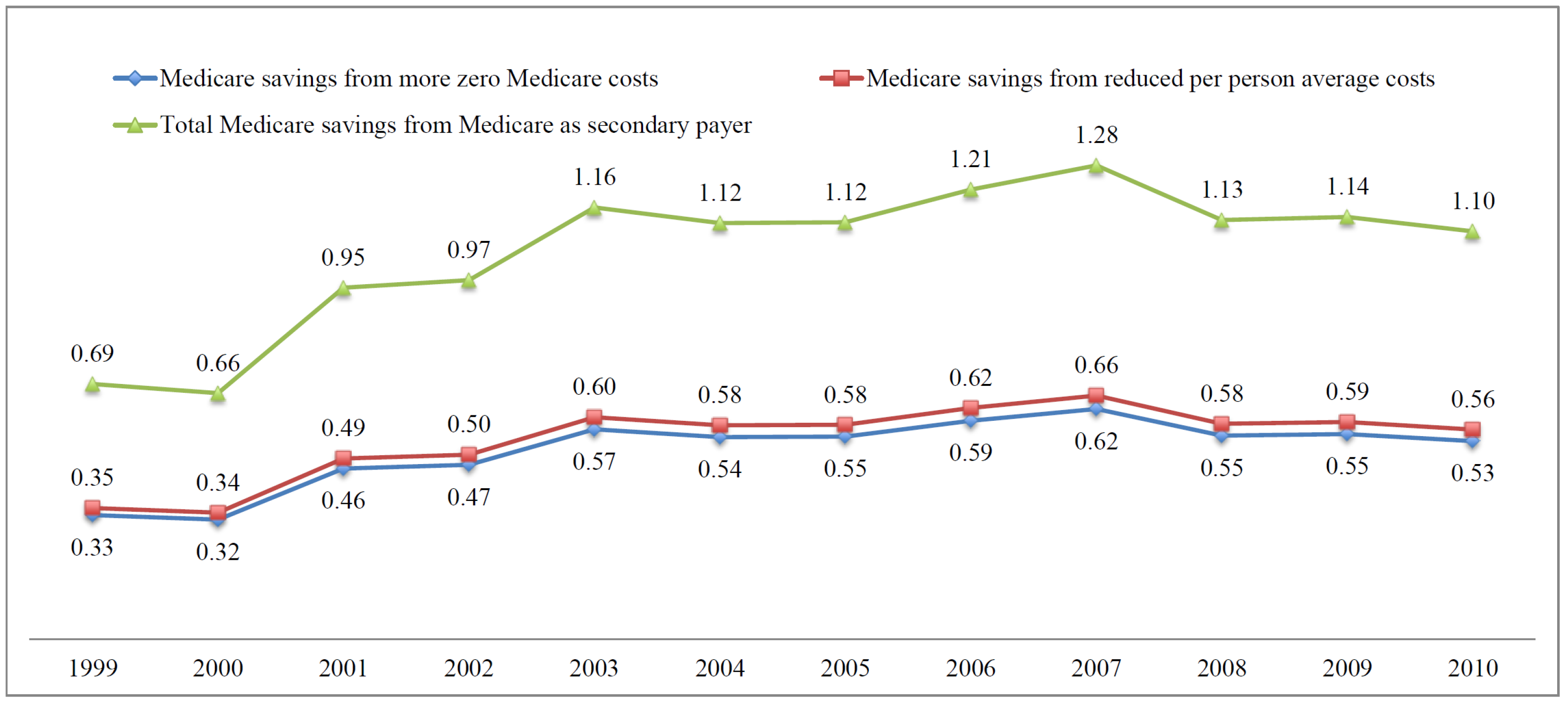
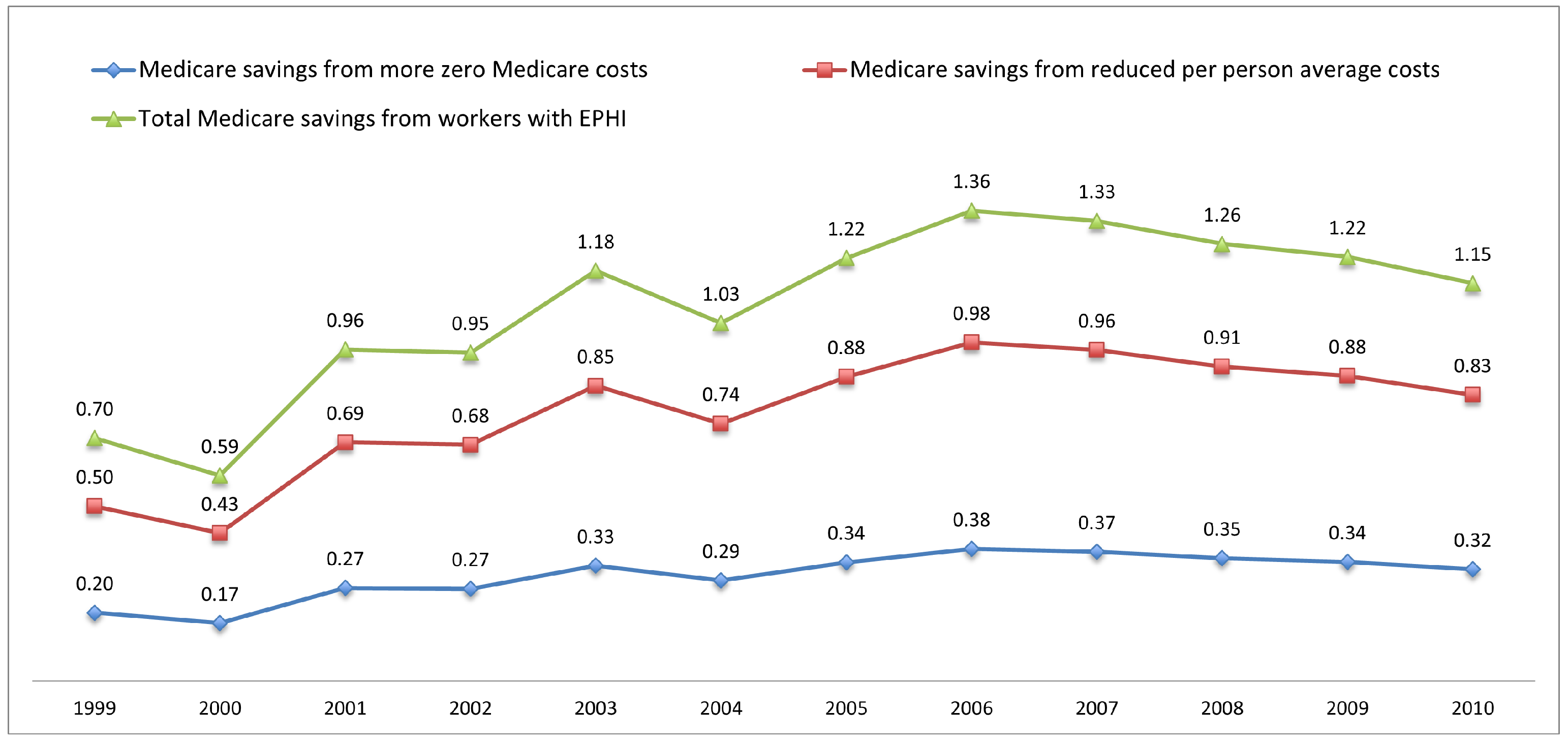
Using the same method we used to calculate the savings from working effect, we also calculate the total Medicare savings due to the fact that, for some individuals, Medicare is the secondary payer. The average annual savings amount during the 1999–2010 period is $1.04 billion. Finally, Table 8 also shows the third part of the Medicare cost savings from workers covered by EPHI, which is captured by the interaction indicator, . The average annual savings amount is about $1.08 billion. To sum up, the aggregate average annual savings amount in the 1999–2010 period related to individuals’ work, MSP, and the joint effects of these items is about $5.37 billion, which represents savings of 1.12 percent of the total Medicare Personal Health Care in 2010.18
Glied and Stabile (2001) discuss estimates of the MSP effect using the 1977 and 1987 National Medicare Expenditure Surveys, and aggregate statistics of work and insurance coverage, which move between half a percent and up to 1 percent of the Medicare expenditure. Considering the different sources of data used, the different time periods analyzed, and the fact that their calculations ignore the differential effect of work and insurance, their estimates are in the ballpark of our findings. On the other hand, Goda et al. (2007) estimate savings for the Medicare system of the MSP provision using Medicare claims data from 1989–1997, and average Medicare expenditure from 1997–2005, to be $11.6 billion for 2002 (which would be closer to 4.5 percent of the total Medicare Personal Health Care in that year, taking the nominal values reported by the authors and CMS). Goda et al. (2007) acknowledge that their calculations are an upper bound, given the type of data they use, and especially the fact that they use aggregate measures of labor supply and insurance to accompany the older expenditure data. Goda et al. (2007) share the limitations of Glied and Stabile (2001), including the fact that they ignore the issue of delays in Medicare enrollment.
Figure 2, Figure 3 and Figure 4 plot Medicare savings from working, MSP, and joint effects respectively. We see an increasing trend of savings in all figures. Working generates higher savings to the Medicare system, compared to MSP and joint effects. The aggregate savings amount from all three sources is $3.45 billion in 1999 and $6.12 billion in 2010.
We investigate whether this trend is just the product of the larger aged population, increased labor force participation, or increases in average Medicare costs. We find that most of the changes can be explained by a combination of the increase in the number of older Americans and the increase in labor force participation; in many years, this accounts for between 70 percent and 80 percent of the changes in savings.
5.2. Medicare Savings from Delayed Medicare Enrollment
In Table 4 and Table 5, indicators of Medicare current and past delayers are used to estimate the Medicare cost savings in each year. The total savings are the sum of savings from past delayers, current Part A or Part B delayers, as well as from Part B delayers covered by EPHI. Appendix A Table A7 shows the detailed breakdown of delayers from years 2004–2010. Using similar calculations to those described earlier, we compute the annual Medicare cost savings from delays in Medicare enrollment. We use the results from both the first and second stage to calculate the corresponding savings. The first stage of Table 4 and Table 5 are included in Appendix A.2. Notice that not all the coefficients on the delay dummies are negative. As a result, instead of generating Medicare cost savings, those positive coefficients generate more costs to the Medicare system. Our calculations using information in Appendix A Table A7 take that into account. The average annual Medicare savings from the number of past delayers (who have delayed both Part A and Part B before) during the 1999–2010 period are about $0.23 billion; the corresponding annual Medicare savings from current Part A delayers, current Part B delayers, as well as Part B delayers covered by EPHI, over 1999–2010, are $0.16 billion, $0.12 billion, and $0.07 billion, respectively.
Our analysis of the effect of enrollment delay has so far focused on the differential effect of having been a past delayer on the observed costs after enrollment, but has not been able to capture the savings to the government in the years in which the individual was not generating any cost to the system. Table 9 shows the retrospective counting of Medicare cost savings from delayed enrollment to approximate these savings. As discussed in Section 2.2, we retrospectively count the number of individuals who have delayed either Part A or Part B or both, in each year, starting in 1999, using all the information regarding enrollment available in the MCBS. We then multiply the number of delayers in each year by the corresponding average Medicare costs to get the numbers shown in Table 9. The details are as follows: we first count the number of individuals who have delayed Part A in 1999 and then use the cross-section sample weights to get the population corresponding to the raw counting. Finally, we multiply the population by the average Medicare Part A costs in 1999 to calculate the savings from those who have delayed Part A in 1999, which is about $2.51 billion. Per Table 9, the Medicare cost savings from retrospective counting are quite large, especially for those who have delayed Part B or both parts. The aggregate Medicare cost savings are around $11.4 billion in 1999 and about $4.98 billion in 2009. The average annual Medicare cost savings are around $9.59 billion during the 1999–2009 period. This amount is about 2 percent of the total Medicare Personal Health Care in 2010. It is important to emphasize that the lower estimated savings in recent years are an artifact of the retrospective perspective. For example, to compute those delaying in 2008, we have data on those who delayed in 2008 and enrolled in 2009 or 2010, but not on those who delayed in 2008 and continued to do so in 2009 and 2010. For earlier years, such as 2004 or 2005, our retrospective calculations are likely accurate, but the estimated savings for recent years is likely a large underestimation of the true savings due to delays in Medicare enrollment. This means that as large as the estimated effect of delay is, the true savings are likely larger, and access to future data will allow us to verify this contention.
Our findings regarding the effects of delayed enrollment in Medicare cannot be compared with similar research since delay behavior has thus far been understudied. Sloan et al. (2012) discuss delay behavior within the Medicare program, but they focus on delay in usage of Medicare Part B services among enrollees, and not on delayed enrollment into the Medicare system. We take their measure of delay into account in our analysis, in that we model that individuals can generate a zero expenditure for the Medicare system. Additionally, Sloan et al. (2012) try to understand the characteristics of individuals who delay usage of Medicare Part B services, but they do not discuss the cost consequences of this behavior for the Medicare system, or the likely connection of delay usage with the availability of EPHI. Sloan et al. (2012) do account for the role of previous health insurance status, but not current health insurance coverage other than Medicare. Notice that, in our data, the weighted percentage of current Part B delayers covered by EPHI is close to 32 percent, which suggests that, in order to understand delay behavior, it is important to account for current insurance coverage.
6. Conclusions
Changes in the U.S. Social Security System, such as increases in the FRA and the DRC and changes in the debt structure of older American households, as well as the increased longevity of Americans, have led to a considerable increase in labor supply in the last couple of decades. Given the connection between work and EPHI coverage, it has become even more important to understand how work and health insurance coverage affect Medicare costs.
In this research we use MCBS individual-level data to identify and estimate the relationship between EPHI, employment, delays in Medicare enrollment, and Medicare costs among aged Medicare beneficiaries. We then use our empirical findings to calculate the Medicare cost savings with regard to three aspects: (1) the savings resulting from the existence of the MSP provision; (2) the savings from individuals working, as an effect independent of insurance status; and (3) the savings from individuals’ delay behaviors. This endeavor is not only innovative, but also essential to understand how a number of recent developments affecting older Americans influence the Medicare system.
Our findings indicate that MSP and being employed (as well as their interaction) are associated with a lower probability of observing positive Medicare spending, and a lower level of Medicare spending. Specifically, MSP (being employed) significantly lowers the probability of Medicare costs by 5.5 (7.5) percent and the level of Medicare spending by 7.6 (10.8) percent. Our extensive sensitivity analysis suggests that our preferred specification provides conservative estimates of the effects.
Using our empirical findings, we calculate that, over the 1999–2010 period, the annual Medicare savings resulting from the fact that around 4.58 million older Americans keep working after age 65, are $3.25 billion. The annual savings amount from MSP for around 1.23 million Americans is around $1.04 billion. Finally, the annual savings from the joint effect of working and MSP for around 0.80 million Americans amount to around $1.08 billion. Most of the changes in these savings over time are linked to increases in the age-eligible Medicare population, and increases in their labor force participation.
To put this set of results in perspective, it is fair to ask whether the savings for the Medicare program resulting from MSP translate into savings for the economy as a whole in terms of health care expenditures. The MCBS does provide data on the health expenditures by individuals who are covered by private insurers if they are also enrolled in Medicare. This means that the total health expenditure measure we show throughout the paper includes those costs. In Table 1, through a simple comparison conditional on just a few characteristics, as well in Table 2 through the study of the probability of observing a positive medical expenditure, and in Table 3, Table 4 and Table 5 through the estimation of our preferred econometric specification, we study the differential effect of EPHI on total health expenditure, and the results indicate that the EPHI indicator is insignificant, which suggests that the savings that we find do not necessarily translate into savings for the whole economy. Recent research by Fronsdal et al. (2020), as well as several references therein, suggests that, for younger individuals, private insurers negotiate higher prices than public programs, but the results are much less clear, and, in many cases, in the other direction, for individuals 65+, which formed our sample. The latter results emerge from the analysis of the differences between individuals who are enrolled on Traditional Medicare versus those enrolled in Medicare Advantage (MA), which is managed by private insurance companies. Given the similarity of these two populations, these results are considered reliable in capturing the effect of the differential coverage on transactions prices. In addition, it is widely believed that private insurance companies are able to reduce usage, resulting in overall lower totals costs even if their negotiated prices are not always lower.
On the other hand, over the same period, the annual Medicare savings resulting from individuals’ delay behavior is $10.17 billion. Ninety-four percent of the savings emerge as a result of our ability to perform retrospective calculations using Medicare enrollment information available in the MCBS.
Overall, the savings we present in this research represent on average around 4 percent of the total Medicare Personal Health Care in the period of analysis, with a range between 3.25 percent and 5.04 percent, depending on the year analyzed.19
Our paper has a number of limitations. First, our savings calculations do not account for delayed enrollment due to death before enrollment in Medicare, which is a cost-saving “silver lining” for the government, nor have we tried to compute these possible savings; to do so, we would have to expand our research to compute the savings or costs linked to early death, as well as longer than expected longevity among those never enrolled and also among those who eventually enroll. A careful analysis of the effects of mortality on Medicare costs is out of the scope of this research, but part of our research agenda. Second, our empirical analysis is conditional on current delay enrollment penalties. Health evolves differently for those who delay and those who do not, since health is a function of delay enrollment decisions. In order to fully understand the consequences of the delay enrollment penalties, the delay enrollment decisions, as well as the underlying evolution of health linked to both, we would need a structural model. That analysis is, again, out of the scope of this research effort but part of our future research. Finally, an important effect of individuals working longer on Medicare finances is the Medicare tax, which would increase revenue to the Medicare system. The quantification of this latter effect is also beyond the scope of this paper but will be a part of our future research.
Owing to the links between employment, health insurance coverage, and Medicare costs presented in this research, our findings may be of interest to policy makers who should take into account the consequences of reforms on the Medicare system. On the other hand, our research is linked with the growing interest to understand the consequences of the role that private insurance companies play in the health coverage of older Americans. Either through the MSP provision, but more strikingly through the emergence of Medicare Advantage (MA), private insurers cover a growing proportion of our seniors, but the jury is still out on whether this is beneficial (in the financial or welfare enhancing sense) to the whole economy given the difficulty in properly observing prices and usage, and how to value the access to additional services offered by MA. In any case, it seems that this trend is unlikely to be reversed regardless of the ultimate answer to that question.
Author Contributions
Conceptualization, Y.D.; Methodology, Y.D. and H.B.-S.; Software, Y.D.; Validation, Y.D. and H.B.-S.; Formal Analysis, Y.D. and H.B.-S.; Investigation, Y.D. and H.B.-S.; Data Curation, Y.D.; Writing—Original Draft Preparation, Y.D. and H.B.-S.; Writing—Review & Editing, Y.D. and H.B.-S.; Visualization, Y.D.; Funding Acquisition, Y.D. and H.B.-S. All authors have read and agreed to the published version of the manuscript.
Funding
Not applicable.
Institutional Review Board Statement
Not applicable.
Informed Consent Statement
Not applicable.
Data Availability Statement
The data presented in this study are not public available. The data presented in this study are administrative data from the Centers for Medicare & Medicaid Services (CMS).
Acknowledgments
We thank Kathleen McGarry for helpful comments, as well as the anonymous referees and editors of the journal for their insightful comments and suggestions. We gratefully acknowledge the financial support from the Michigan Retirement and Disability Research Center (MRDRC) for supporting a related research project through grant [UM15-13], and the financial support from the ARC Centre of Excellence in Population Ageing Research (CEPAR)-CE17010005.
Conflicts of Interest
The authors declare no conflict of interest. The founding sponsors had no role in the design of the study; in the collection, analyses, or interpretation of data; in the writing of the manuscript, and in the decision to publish the results.
Abbreviations
The following abbreviations are used in this manuscript:
| MSP | Medicare as secondary payer |
| MCBS | Medicare Current Beneficiary Survey |
| EPHI | Employer-provided health insurance |
| OOP | Out-of-pocket |
| DRC | Delayed retirement credits |
| FRA | Full retirement age |
| CMS | Centers for Medicare & Medicaid Services |
| LFPR | Labor force participation rate |
| IEP | Initial enrollment period |
| SEP | Special enrollment period |
| OLS | Ordinary least squares |
| TPM | Two-part model |
| IV | Instrumental Variable |
| FE | Fixed-Effect |
| NHIS | National Health Interview Survey |
| HRS | Health and Retirement Study |
| CPI | Consumer Price Index |
| MA | Medicare Advantage |
Appendix A
Appendix A.1. Summary Statistics
In the MCBS, there is only one dummy variable that captures the sample person’s working status, and it takes the value one if the sample person is currently working at a job or business, and zero if they are not working. This variable first became available in 1999, and given that our goal is to link labor market attachment, health insurance coverage, and Medicare costs of elderly individuals around retirement age, the sample used in our analysis covers the 1999–2010 period of the MCBS Cost and Use Files. We restrict our estimation sample to observations linked to individuals who are still alive 6 months after being first observed.20 We further restrict our estimation sample to aged Medicare beneficiaries. Notice that, if a sample person was originally entitled to Medicare due to disability, once they turn 65, they are coded as aged. In order to solve this issue, we construct the enrollment year and enrollment month variables using information on the individual’s date of birth, as well as their Medicare entitlement date. The Medicare 7 months IEP is 3 months before an individual turns 65, the month they turn 65, and 3 months after they turn 65. Sample respondents whose Medicare entitlement age is 64 years and 9 months or older are considered enrolled in Medicare because of aging and are kept in the estimation sample.
We exclude individuals with missing information on working status, health-related variables, demographic variables, and health insurance indicators. We also exclude individuals who are not working but claimed to be covered by employer-provided health insurance through their work (maybe because they were temporarily on leave), and we also exclude individuals who had interviews in facilities.21 Finally, we exclude a small fraction of individuals who changed coverage, since their changes in Medicare costs are naturally connected with this endogenous decision. After all these exclusions, we are left with 95,545 person-year observations.
Owing to the nature of the MCBS, all individuals in the sample have Medicare coverage. In addition, individuals could have one or more types of health insurance coverage other than Medicare. Given that our interest is to look at the effects of EPHI on Medicare costs, we classify individuals into two mutually exclusive health insurance categories: those who have EPHI regardless of other health insurance coverage, and those who do not. The MCBS has a rich set of health measures and some demographic information. The health measures include self-reported health status, activities of daily living, instrumental activities of daily living, cancer, and chronic disease. Self-reported health status takes values one to five, each value corresponding to excellent, very good, good, fair, and poor accordingly. Through the MCBS Cost and Use files we have complete expenditure and source of payment data on all health care services, including those not covered by Medicare. For the purpose of our study, we focus on the following three measures of individuals’ medical expenditure: total health expenditure, Medicare costs, and OOP expenditure.
Table A1 provides some descriptive statistics by EPHI status. There are significant differences between the EPHI and no EPHI subsamples, with those covered by EPHI comparatively younger, more likely to be male and married, comparatively with higher education and in better health, and more than 50 percentage points more likely to be currently working. Age in our estimation is top-coded, meaning that observations aged 90 and over are coded as aged 90.
Table A2 shows the weighted average medical expenditure and premiums in our sample. In general, women generate higher medical costs than men. Individuals with less than 10 years of Social Security-covered employment are those paying the annual Medicare Part A premiums. The amount they pay is $3957 per year, which is more than twice the average OOP expenditure. Around 15 percent of the sample are currently working, and among those, about 17 percent are covered by EPHI. About 4 percent of the estimation sample are covered by EPHI, of which 65 percent are covered by EPHI through their own employment with the rest being covered by EPHI through their spouse’s employment.

Table A1.
Descriptive statistics of selected variables by EPHI.
| Variables | No EPHI | EPHI | All |
|---|---|---|---|
| Age | 75.55 | 70.18 | 75.33 |
| (7.088) | (4.844) | (7.089) | |
| Male | 0.416 | 0.517 | 0.420 |
| (0.493) | (0.500) | (0.494) | |
| Married | 0.554 | 0.751 | 0.562 |
| (0.497) | (0.433) | (0.496) | |
| Black | 0.076 | 0.073 | 0.076 |
| (0.264) | (0.260) | (0.264) | |
| Hispanic | 0.020 | 0.007 | 0.020 |
| (0.141) | (0.083) | (0.139) | |
| High School | 0.300 | 0.242 | 0.297 |
| (0.458) | (0.428) | (0.457) | |
| Some College | 0.252 | 0.286 | 0.254 |
| (0.434) | (0.452) | (0.435) | |
| College | 0.105 | 0.142 | 0.106 |
| (0.306) | (0.350) | (0.309) | |
| Excellent Health | 0.173 | 0.264 | 0.177 |
| (0.379) | (0.441) | (0.382) | |
| Very Good Health | 0.313 | 0.353 | 0.315 |
| (0.464) | (0.478) | (0.465) | |
| Good Health | 0.325 | 0.275 | 0.323 |
| (0.468) | (0.446) | (0.468) | |
| Fair Health | 0.144 | 0.087 | 0.142 |
| (0.352) | (0.283) | (0.349) | |
| Currently Working | 0.129 | 0.652 | 0.151 |
| (0.336) | (0.476) | (0.358) |
Note: Authors’ calculation using the pooled 1999–2010 MCBS Cost and Use files, using cross-sectional sample weights. Standard deviations are in parentheses. Number of observations varies by variable and sample.
Table A2.
Descriptive statistics of selected variables.
| Variables | Female | Male | Total |
|---|---|---|---|
| Premium–A | $3962 | $3954 | $3957 |
| (2011) | (1677) | (1817) | |
| Premium–B | $998 | $1004 | $1001 |
| (234) | (239) | (236) | |
| Medicare Costs | $6782 | $7352 | $7012 |
| (14,309) | (16,407) | (15,193) | |
| Total Health Expenditure | $10,693 | $11,056 | $10,844 |
| (17,465) | (20,026) | (18,576) | |
| OOP Expenditure | $1871 | $1766 | $1827 |
| (4213) | (3895) | (4084) | |
| Income of Respondent | $32,642 | $46,380 | $38,414 |
| (54,373) | (88,417) | (71,027) | |
| Currently Working | 0.114 | 0.202 | 0.151 |
| (0.317) | (0.401) | (0.358) | |
| EPHI among Workers | 0.173 | 0.177 | 0.175 |
| (0.378) | (0.381) | (0.380) | |
| Covered by EPHI | 0.034 | 0.050 | 0.041 |
| (0.181) | (0.218) | (0.197) | |
| Workers among EPHI | 0.583 | 0.717 | 0.652 |
| (0.493) | (0.450) | (0.476) |
Note: Authors’ calculation using data from the pooled 1999–2010 MCBS Cost and Use files, using cross-sectional sample weights. Standard deviations are in parentheses. Number of observations varies by variable and sample.
Appendix A.2. Additional Estimation Results
Here, we present additional estimates for Table 2 and Table A3, Table 3 and Table A4, Table 4 and Table A5, and Table 5 and Table A6. Notice that we include an indicator for being a in Table A3, Table A4, Table A5 and Table A6, that is, respondents who, because of when they were added to the sample, in some cases, had their health care costs imputed in some years. We find that being one of these individuals significantly reduces the probability of seeing positive Medicare costs, and reduces the Medicare costs conditional on the positive costs. It is unclear why this indicator is significant, except that the need for imputation of some of the variables seems to have been short of random in the sample of analysis.
Table A3.
Regression of probability of positive medical spending on work and EPHI.
| Variables | Medicare Costs | Total Health Exp. | Out-of-Pocket Exp. |
|---|---|---|---|
| Ghost | −0.024 | −0.006 | −0.005 |
| (0.008) | (0.003) | (0.003) | |
| Good Health | 0.019 | 0.007 | 0.010 |
| (0.003) | (0.001) | (0.002) | |
| Fair Health | 0.039 | 0.011 | 0.011 |
| (0.005) | (0.002) | (0.002) | |
| Poor Health | 0.043 | 0.004 | 0.001 |
| (0.009) | (0.005) | (0.004) | |
| Age | 0.126 | 0.008 | 0.014 |
| (0.008) | (0.003) | (0.003) | |
| Age | −0.001 | −0.000 | −0.000 |
| (0.000) | (0.000) | (0.000) | |
| Ever Smoke | −0.001 | 0.000 | 0.002 |
| (0.004) | (0.001) | (0.002) | |
| Smoker | −0.033 | −0.012 | −0.017 |
| (0.005) | (0.002) | (0.002) | |
| No Schooling | 0.021 | −0.009 | −0.022 |
| (0.018) | (0.005) | (0.005) | |
| Less than 8th | −0.019 | −0.007 | −0.012 |
| (0.006) | (0.002) | (0.002) | |
| Some High School | −0.009 | −0.004 | −0.006 |
| (0.006) | (0.002) | (0.002) | |
| Some College | 0.001 | 0.004 | 0.005 |
| (0.005) | (0.002) | (0.002) | |
| College | 0.022 | 0.008 | 0.013 |
| (0.007) | (0.003) | (0.003) | |
| Graduate School | 0.036 | 0.011 | 0.017 |
| (0.007) | (0.003) | (0.004) | |
| Widow | −0.009 | −0.005 | −0.005 |
| (0.004) | (0.002) | (0.002) | |
| Separated | −0.040 | −0.008 | −0.013 |
| (0.016) | (0.005) | (0.005) | |
| Never Married | −0.017 | −0.013 | −0.017 |
| (0.010) | (0.003) | (0.004) | |
| Black | −0.069 | −0.011 | −0.013 |
| (0.006) | (0.002) | (0.002) | |
| Hispanic | −0.056 | −0.000 | −0.023 |
| (0.011) | (0.004) | (0.004) | |
| Other Race | −0.010 | −0.006 | −0.017 |
| (0.011) | (0.003) | (0.004) | |
| Number of Kids | −0.000 | −0.000 | −0.001 |
| (0.001) | (0.000) | (0.000) | |
| Male | −0.043 | −0.013 | −0.016 |
| (0.004) | (0.001) | (0.002) | |
| Income 10 K–15 K | −0.031 | 0.006 | 0.016 |
| (0.006) | (0.002) | (0.002) | |
| Income 15 K–20 K | −0.017 | 0.010 | 0.023 |
| (0.006) | (0.002) | (0.002) | |
| Income 20 K–25 K | −0.009 | 0.012 | 0.029 |
| (0.007) | (0.002) | (0.003) | |
| Income 25 K–30 K | −0.007 | 0.014 | 0.031 |
| (0.007) | (0.002) | (0.003) | |
| Income 30 K–35 K | 0.010 | 0.021 | 0.039 |
| (0.007) | (0.003) | (0.003) | |
| Income 35 K–40 K | 0.019 | 0.020 | 0.038 |
| (0.008) | (0.003) | (0.003) | |
| Income 40 K–45 K | 0.028 | 0.024 | 0.048 |
| (0.009) | (0.003) | (0.004) | |
| Income 45 K–50 K | 0.036 | 0.025 | 0.046 |
| (0.009) | (0.003) | (0.004) | |
| Income 50 K+ | 0.030 | 0.031 | 0.052 |
| (0.007) | (0.003) | (0.003) | |
| Mid–West | 0.075 | 0.003 | 0.002 |
| (0.005) | (0.002) | (0.002) | |
| South | 0.065 | 0.000 | −0.001 |
| (0.005) | (0.002) | (0.002) | |
| West | −0.071 | −0.001 | −0.006 |
| (0.005) | (0.002) | (0.002) | |
| had_hbp | 0.045 | 0.022 | 0.029 |
| (0.004) | (0.001) | (0.002) | |
| had_diabts | 0.019 | 0.016 | 0.018 |
| (0.005) | (0.002) | (0.002) | |
| had_emphys | 0.021 | 0.012 | 0.013 |
| (0.005) | (0.002) | (0.003) | |
| had_myocar | 0.013 | 0.006 | 0.008 |
| (0.006) | (0.002) | (0.003) | |
| had_chd | 0.016 | 0.011 | 0.009 |
| (0.006) | (0.003) | (0.003) | |
| had_stroke | 0.008 | 0.008 | 0.008 |
| (0.006) | (0.003) | (0.003) | |
| had_psych | −0.009 | 0.007 | 0.002 |
| (0.007) | (0.004) | (0.004) | |
| had_alzhmr | 0.019 | 0.011 | 0.008 |
| (0.010) | (0.006) | (0.005) | |
| had_brkhip | −0.021 | −0.003 | −0.002 |
| (0.009) | (0.004) | (0.004) | |
| had_arth | 0.030 | 0.013 | 0.014 |
| (0.004) | (0.001) | (0.002) | |
| had_cancer | 0.028 | 0.014 | 0.016 |
| (0.004) | (0.002) | (0.002) | |
| had_ctarac | 0.037 | 0.009 | 0.009 |
| (0.004) | (0.002) | (0.002) | |
| had_hraid | −0.001 | 0.011 | 0.016 |
| (0.006) | (0.003) | (0.003) | |
| diff_walkblks | 0.006 | 0.002 | 0.004 |
| (0.004) | (0.002) | (0.002) | |
| diff_walkblks_nr | −0.014 | 0.016 | 0.014 |
| (0.029) | (0.012) | (0.012) | |
| diff_stoop | 0.017 | 0.002 | 0.005 |
| (0.004) | (0.001) | (0.002) | |
| diff_stoop_nr | 0.129 | 0.000 | 0.018 |
| (0.068) | (.) | (0.033) | |
| diff_reach | 0.019 | −0.000 | 0.003 |
| (0.004) | (0.002) | (0.002) | |
| diff_reach_nr | −0.100 | 0.001 | −0.004 |
| (0.051) | (0.019) | (0.020) | |
| diff_lift | 0.013 | 0.005 | 0.000 |
| (0.004) | (0.002) | (0.002) | |
| diff_lift_nr | 0.035 | −0.029 | −0.026 |
| (0.043) | (0.012) | (0.016) | |
| diff_dres | −0.006 | −0.001 | 0.000 |
| (0.012) | (0.006) | (0.006) | |
| diff_walk | −0.010 | 0.000 | 0.000 |
| (0.005) | (0.002) | (0.002) | |
| diff_bath | −0.002 | 0.001 | 0.003 |
| (0.008) | (0.004) | (0.005) | |
| diff_eat | −0.015 | 0.001 | −0.009 |
| (0.013) | (0.007) | (0.005) | |
| diff_char | −0.000 | −0.003 | −0.004 |
| (0.006) | (0.003) | (0.003) | |
| diff_toil | −0.003 | −0.004 | 0.007 |
| (0.010) | (0.005) | (0.005) | |
| diff_meal | 0.003 | 0.004 | 0.002 |
| (0.007) | (0.003) | (0.003) | |
| diff_shop | 0.002 | −0.004 | −0.007 |
| (0.009) | (0.004) | (0.004) | |
| diff_tele | −0.010 | −0.013 | −0.009 |
| (0.008) | (0.003) | (0.004) | |
| diff_bils | 0.017 | −0.002 | 0.002 |
| (0.009) | (0.004) | (0.004) | |
| help_dres | −0.007 | 0.029 | 0.006 |
| (0.016) | (0.011) | (0.007) | |
| help_walk | −0.007 | 0.004 | −0.000 |
| (0.010) | (0.006) | (0.005) | |
| help_bath | 0.018 | 0.001 | −0.002 |
| (0.012) | (0.006) | (0.006) | |
| help_eat | 0.071 | −0.020 | 0.006 |
| (0.024) | (0.010) | (0.009) | |
| help_chair | 0.013 | 0.012 | 0.004 |
| (0.013) | (0.007) | (0.007) | |
| help_toil | 0.028 | −0.012 | −0.007 |
| (0.018) | (0.008) | (0.008) | |
| help_meal | −0.001 | 0.006 | −0.006 |
| (0.010) | (0.005) | (0.005) | |
| help_shop | −0.004 | −0.002 | 0.001 |
| (0.010) | (0.005) | (0.005) | |
| help_tele | 0.013 | 0.009 | 0.006 |
| (0.012) | (0.005) | (0.005) | |
| help_bills | −0.018 | 0.004 | 0.007 |
| (0.011) | (0.006) | (0.006) | |
| drc35 | 0.075 | 0.008 | 0.011 |
| (0.007) | (0.003) | (0.003) | |
| drc40 | 0.107 | 0.008 | 0.011 |
| (0.008) | (0.003) | (0.003) | |
| drc45 | 0.155 | 0.004 | 0.015 |
| (0.008) | (0.003) | (0.004) | |
| drc50 | 0.188 | 0.009 | 0.023 |
| (0.009) | (0.003) | (0.004) | |
| drc55 | 0.227 | 0.005 | 0.022 |
| (0.009) | (0.003) | (0.004) | |
| drc60 | 0.279 | 0.007 | 0.025 |
| (0.010) | (0.004) | (0.004) | |
| drc65 | 0.314 | 0.007 | 0.025 |
| (0.012) | (0.004) | (0.005) | |
| drc65_fra2 | 0.334 | 0.005 | 0.023 |
| (0.013) | (0.004) | (0.005) | |
| drc70_fra4 | 0.345 | 0.008 | 0.029 |
| (0.013) | (0.004) | (0.005) | |
| drc70_fra6 | 0.342 | 0.011 | 0.031 |
| (0.014) | (0.005) | (0.006) | |
| drc75_fra8 | 0.394 | 0.006 | 0.030 |
| (0.015) | (0.005) | (0.006) | |
| drc75_fra10 | 0.377 | 0.008 | 0.032 |
| (0.017) | (0.006) | (0.007) | |
| drc80_fra66 | 0.361 | 0.000 | 0.021 |
| (0.013) | (0.005) | (0.006) |
Note: Authors’ calculation using data from the pooled 1999–2010 MCBS Cost and Use files. This table shows additional variables from regressions of probability of positive medical expenses on work and MSP. Robust standard errors, clustered at the individual level, are in parentheses.
Table A4.
Regression of level of medical spending on work and EPHI.
| Variables | Medicare Costs | Total Health Exp. | Out-of-Pocket Exp. |
|---|---|---|---|
| Ghost | −0.139 | −0.210 | −0.203 |
| (0.035) | (0.035) | (0.022) | |
| Good Health | 0.314 | 0.233 | 0.161 |
| (0.014) | (0.015) | (0.009) | |
| Fair Health | 0.515 | 0.396 | 0.213 |
| (0.019) | (0.021) | (0.013) | |
| Poor Health | 0.896 | 0.627 | 0.225 |
| (0.031) | (0.034) | (0.021) | |
| Age | 0.193 | 0.178 | 0.124 |
| (0.022) | (0.024) | (0.015) | |
| Age | −0.001 | −0.001 | −0.001 |
| (0.000) | (0.000) | (0.000) | |
| Ever Smoke | 0.072 | 0.046 | 0.016 |
| (0.013) | (0.014) | (0.009) | |
| Smoker | −0.211 | −0.174 | −0.145 |
| (0.022) | (0.023) | (0.015) | |
| No Schooling | −0.072 | −0.084 | −0.586 |
| (0.054) | (0.058) | (0.038) | |
| Less than 8th | −0.088 | −0.133 | −0.228 |
| (0.021) | (0.022) | (0.014) | |
| Some High School | −0.078 | −0.065 | −0.079 |
| (0.019) | (0.020) | (0.012) | |
| Some College | 0.066 | 0.043 | 0.071 |
| (0.016) | (0.017) | (0.011) | |
| College | 0.070 | 0.088 | 0.176 |
| (0.022) | (0.023) | (0.015) | |
| Graduate School | 0.086 | 0.155 | 0.219 |
| (0.025) | (0.026) | (0.017) | |
| Widow | 0.066 | 0.056 | 0.045 |
| (0.015) | (0.016) | (0.010) | |
| Divorced | 0.064 | 0.015 | −0.033 |
| (0.024) | (0.025) | (0.016) | |
| Separated | 0.145 | 0.006 | −0.188 |
| (0.070) | (0.072) | (0.047) | |
| Never Married | −0.037 | −0.023 | −0.102 |
| (0.037) | (0.040) | (0.025) | |
| Black | 0.036 | −0.096 | −0.287 |
| (0.024) | (0.024) | (0.016) | |
| Hispanic | 0.011 | −0.194 | −0.468 |
| (0.043) | (0.044) | (0.029) | |
| Other Race | 0.045 | −0.059 | −0.511 |
| (0.039) | (0.040) | (0.026) | |
| Number of Kids | 0.000 | 0.001 | −0.008 |
| (0.003) | (0.003) | (0.002) | |
| Male | 0.054 | −0.003 | −0.151 |
| (0.014) | (0.015) | (0.010) | |
| Income 10 K–15 K | −0.003 | 0.002 | 0.412 |
| (0.023) | (0.025) | (0.016) | |
| Income 15 K–20 K | 0.012 | 0.051 | 0.579 |
| (0.025) | (0.027) | (0.018) | |
| Income 20 K–25 K | −0.001 | 0.093 | 0.655 |
| (0.026) | (0.028) | (0.019) | |
| Income 25 K–30 K | 0.064 | 0.156 | 0.699 |
| (0.027) | (0.029) | (0.019) | |
| Income 30 K–35 K | 0.020 | 0.127 | 0.691 |
| (0.029) | (0.032) | (0.021) | |
| Income 35 K–40 K | 0.073 | 0.206 | 0.729 |
| (0.030) | (0.032) | (0.021) | |
| Income 40 K–45 K | 0.087 | 0.240 | 0.763 |
| (0.033) | (0.036) | (0.024) | |
| Income 45 K–50 K | 0.090 | 0.265 | 0.790 |
| (0.034) | (0.037) | (0.024) | |
| Income 50 K+ | 0.152 | 0.305 | 0.880 |
| (0.026) | (0.029) | (0.019) | |
| Mid–West | −0.204 | −0.043 | 0.080 |
| (0.019) | (0.019) | (0.012) | |
| South | −0.139 | −0.016 | 0.128 |
| (0.017) | (0.017) | (0.011) | |
| West | −0.101 | −0.217 | −0.056 |
| (0.021) | (0.020) | (0.013) | |
| had_hbp | 0.099 | 0.194 | 0.198 |
| (0.013) | (0.015) | (0.010) | |
| had_diabts | 0.293 | 0.250 | 0.214 |
| (0.015) | (0.016) | (0.010) | |
| had_emphys | 0.275 | 0.251 | 0.142 |
| (0.017) | (0.018) | (0.011) | |
| had_myocar | 0.226 | 0.214 | 0.113 |
| (0.018) | (0.019) | (0.012) | |
| had_chd | 0.260 | 0.213 | 0.135 |
| (0.018) | (0.020) | (0.013) | |
| had_stroke | 0.168 | 0.156 | 0.121 |
| (0.018) | (0.020) | (0.013) | |
| had_psych | 0.137 | 0.147 | 0.184 |
| (0.025) | (0.026) | (0.017) | |
| had_alzhmr | 0.017 | 0.072 | 0.103 |
| (0.032) | (0.035) | (0.022) | |
| had_brkhip | 0.267 | 0.184 | 0.073 |
| (0.030) | (0.032) | (0.020) | |
| had_arth | 0.130 | 0.120 | 0.088 |
| (0.013) | (0.014) | (0.009) | |
| had_cancer | 0.328 | 0.234 | 0.137 |
| (0.012) | (0.013) | (0.008) | |
| had_ctarac | 0.102 | 0.114 | 0.055 |
| (0.013) | (0.014) | (0.009) | |
| had_hraid | 0.096 | 0.174 | 0.283 |
| (0.018) | (0.020) | (0.012) | |
| diff_walkblks | 0.219 | 0.166 | 0.085 |
| (0.016) | (0.017) | (0.011) | |
| diff_walkblks_nr | −0.012 | −0.077 | 0.034 |
| (0.127) | (0.136) | (0.085) | |
| diff_stoop | 0.059 | 0.074 | 0.063 |
| (0.015) | (0.016) | (0.010) | |
| diff_stoop_nr | 0.009 | 0.115 | 0.123 |
| (0.273) | (0.299) | (0.191) | |
| diff_reach | −0.020 | 0.010 | 0.009 |
| (0.015) | (0.016) | (0.010) | |
| diff_reach_nr | 0.478 | −0.006 | −0.198 |
| (0.271) | (0.283) | (0.182) | |
| diff_lift | 0.184 | 0.138 | 0.047 |
| (0.016) | (0.017) | (0.011) | |
| diff_lift_nr | −0.060 | 0.336 | 0.090 |
| (0.177) | (0.195) | (0.124) | |
| diff_dres | −0.008 | −0.012 | −0.021 |
| (0.044) | (0.048) | (0.030) | |
| diff_walk | 0.096 | 0.082 | 0.088 |
| (0.019) | (0.021) | (0.013) | |
| diff_bath | 0.056 | 0.047 | 0.027 |
| (0.032) | (0.035) | (0.022) | |
| diff_eat | −0.035 | −0.007 | 0.062 |
| (0.051) | (0.055) | (0.035) | |
| diff_char | −0.087 | −0.049 | −0.018 |
| (0.025) | (0.027) | (0.017) | |
| diff_toil | 0.003 | 0.064 | 0.100 |
| (0.037) | (0.041) | (0.025) | |
| diff_meal | 0.133 | 0.051 | −0.006 |
| (0.026) | (0.028) | (0.018) | |
| diff_shop | 0.030 | 0.036 | −0.002 |
| (0.036) | (0.040) | (0.025) | |
| diff_tele | −0.210 | −0.101 | −0.025 |
| (0.032) | (0.034) | (0.022) | |
| diff_bils | 0.024 | 0.043 | 0.033 |
| (0.034) | (0.037) | (0.023) | |
| help_dres | 0.037 | 0.017 | 0.054 |
| (0.057) | (0.062) | (0.039) | |
| help_walk | 0.023 | −0.007 | −0.059 |
| (0.037) | (0.041) | (0.026) | |
| help_bath | 0.324 | 0.229 | 0.061 |
| (0.043) | (0.048) | (0.030) | |
| help_eat | 0.120 | 0.224 | 0.033 |
| (0.080) | (0.089) | (0.056) | |
| help_chair | −0.024 | 0.002 | 0.022 |
| (0.049) | (0.054) | (0.034) | |
| help_toil | 0.137 | 0.111 | 0.027 |
| (0.064) | (0.071) | (0.044) | |
| help_meal | 0.053 | 0.049 | −0.000 |
| (0.037) | (0.041) | (0.026) | |
| help_shop | 0.092 | 0.078 | 0.025 |
| (0.040) | (0.044) | (0.028) | |
| help_tele | −0.033 | −0.029 | 0.058 |
| (0.042) | (0.046) | (0.029) | |
| help_bills | −0.059 | −0.058 | −0.005 |
| (0.042) | (0.046) | (0.029) | |
| constant | −0.877 | 0.703 | 0.831 |
| (0.877) | (0.939) | (0.592) |
Note: Authors’ calculation using data from the pooled 1999–2010 MCBS Cost and Use files. This table shows additional variables from regressions of level of medical expenses on work and MSP. Standard errors are in parentheses.
Table A5.
Regression of probability of positive medical spending on current delayed enrollment.
| (1) With Health Controls | (2) Without Health Controls | |||||
|---|---|---|---|---|---|---|
| Medicare | Total | OOP | Medicare | Total | OOP | |
| Work | −0.030 | 0.002 | 0.001 | −0.033 | 0.001 | 0.001 |
| (0.005) | (0.002) | (0.002) | (0.005) | (0.002) | (0.002) | |
| EPHI | 0.002 | 0.001 | 0.008 | 0.002 | 0.001 | 0.008 |
| (0.014) | (0.006) | (0.008) | (0.014) | (0.006) | (0.008) | |
| wepc | −0.003 | 0.004 | 0.001 | −0.002 | 0.004 | 0.002 |
| (0.017) | (0.007) | (0.009) | (0.017) | (0.007) | (0.009) | |
| Delay–A–current | 0.112 | −0.000 | −0.047 | 0.113 | 0.000 | −0.047 |
| (0.019) | (0.006) | (0.005) | (0.019) | (0.006) | (0.005) | |
| Delay–B–current | −0.460 | −0.017 | −0.019 | −0.460 | −0.017 | −0.019 |
| (0.011) | (0.003) | (0.004) | (0.011) | (0.003) | (0.004) | |
| EPHI–B–current | −0.093 | 0.003 | −0.002 | −0.093 | 0.003 | −0.002 |
| (0.026) | (0.006) | (0.009) | (0.026) | (0.006) | (0.009) | |
| Good Health | 0.020 | 0.007 | 0.010 | |||
| (0.003) | (0.001) | (0.002) | ||||
| Fair Health | 0.037 | 0.011 | 0.011 | |||
| (0.005) | (0.002) | (0.002) | ||||
| Poor Health | 0.039 | 0.004 | 0.002 | |||
| (0.008) | (0.005) | (0.004) | ||||
| Obs. | 95,146 | 95,103 | 95,146 | 95,146 | 95,103 | 95,146 |
Note: Authors’ calculation using data from the pooled 1999–2010 MCBS Cost and Use files. This table shows the estimates from regressions of medical expenses on work, MSP, and current delayed enrollment. All regressions also contain (but are not reported in the table): ghost indicator, age, age squared, health controls, smoking indicators, number of kids, income-level dummies, race, education, marital status, and census region dummies. Robust standard errors, clustered at the individual level, are in parentheses.
Table A6.
Regression of probability of positive medical spending on current and past delayed enrollment.
Table A6.
Regression of probability of positive medical spending on current and past delayed enrollment.
| (1) With Health Controls | (2) Without Health Controls | |||||
|---|---|---|---|---|---|---|
| Medicare | Total | OOP | Medicare | Total | OOP | |
| Work | −0.031 | 0.002 | 0.001 | −0.033 | 0.002 | 0.001 |
| (0.005) | (0.002) | (0.002) | (0.005) | (0.002) | (0.002) | |
| EPHI | 0.002 | 0.001 | 0.008 | 0.002 | 0.001 | 0.008 |
| (0.014) | (0.006) | (0.008) | (0.014) | (0.006) | (0.008) | |
| wepc | −0.003 | 0.004 | 0.001 | −0.002 | 0.004 | 0.002 |
| (0.017) | (0.007) | (0.009) | (0.017) | (0.007) | (0.009) | |
| Delay–A–current | 0.114 | −0.001 | −0.048 | 0.115 | −0.000 | −0.048 |
| (0.019) | (0.006) | (0.005) | (0.019) | (0.006) | (0.005) | |
| Delay–B–current | −0.459 | −0.017 | −0.019 | −0.459 | −0.017 | −0.019 |
| (0.011) | (0.003) | (0.004) | (0.011) | (0.003) | (0.004) | |
| EPHI–B–current | −0.093 | 0.003 | −0.002 | −0.093 | 0.003 | −0.002 |
| (0.026) | (0.006) | (0.009) | (0.026) | (0.006) | (0.009) | |
| Delay–past | 0.021 | −0.003 | −0.009 | 0.021 | −0.003 | −0.009 |
| (0.011) | (0.004) | (0.004) | (0.011) | (0.004) | (0.004) | |
| Good Health | 0.019 | 0.007 | 0.010 | |||
| (0.003) | (0.001) | (0.002) | ||||
| Fair Health | 0.037 | 0.011 | 0.011 | |||
| (0.005) | (0.002) | (0.002) | ||||
| Poor Health | 0.039 | 0.004 | 0.002 | |||
| (0.008) | (0.005) | (0.004) | ||||
| Obs. | 95,146 | 95,103 | 95,146 | 95,146 | 95,103 | 95,146 |
Note: Authors’ calculation using data from the pooled 1999–2010 MCBS Cost and Use files. This table shows the estimates from regressions of medical expenses on work, MSP, current, and past delayed enrollment. All regressions also contain (but are not reported in the table): ghost indicator, age, age squared, health controls, smoking indicators, number of kids, income-level dummies, race, education, marital status, and census region dummies. Robust standard errors, clustered at the individual level, are in parentheses.
Appendix A.3. Medicare Savings
To compute the effect of work and EPHI on the probability of observing positive Medicare costs, we can take the results directly from Table 2. From the marginal effects of , and , as well as the predicted weighted average probability of having positive Medicare costs, which is 81 percent, we find that the variable decreases the average probability of observing positive Medicare costs by around 6.79 percent (5.5 percent divided by 81 percent), while the variable decreases the average probability of observing positive Medicare costs by around 9.26 percent (7.5 percent divided by 81 percent). Additionally, we have to take into account the interaction term, , which further decreases the probability of observing positive Medicare costs by around 9.88 percent (8 percent divided by 81 percent). From the results of the second stage, shown in Table 3, the coefficients of and are also negative and statistically significantly correlated with the level of Medicare costs. We find that workers spend 7.6 percent less than non-workers. Those who are covered by EPHI and, therefore, have MSP, spend on average 10.8 percent less than those with Medicare as primary payer. Finally, those who work and have EPHI further decrease the average Medicare costs by 28.1 percent.
Table A7.
Population (in millions) by delay status and year.
| Year | 2004 | 2005 | 2006 | 2007 | 2008 | 2009 | 2010 |
|---|---|---|---|---|---|---|---|
| Past Delayers | 0.85 | 0.75 | 0.78 | 0.83 | 0.77 | 0.77 | 0.81 |
| Medicare ≻ 0 | 81.4% | 79.6% | 92.2% | 95.1% | 96.8% | 98.5% | 94.5% |
| Medicare = 0 | 18.6% | 20.4% | 7.8% | 4.9% | 3.2% | 1.5% | 5.5% |
| Prob(Medicare ≻ 0) | 79.3% | 77.5% | 89.8% | 92.6% | 94.3% | 95.9% | 92% |
| Diff. of prob. | 2.11% | 2.06% | 2.39% | 2.46% | 2.51% | 2.55% | 2.45% |
| Avg. Medicare costs | $7291 | $7308 | $7159 | $7253 | $7007 | $6702 | $6673 |
| Current Part A delayers | 0.26 | 0.25 | 0.21 | 0.16 | 0.19 | 0.23 | 0.24 |
| Medicare ≻ 0 | 86.2% | 96.3% | 96.5% | 97.6% | 100% | 94.9% | 95.5% |
| Medicare = 0 | 13.8% | 3.7% | 3.5% | 2.4% | 0.0% | 5.1% | 4.5% |
| Prob(Medicare ≻ 0) | 74.3% | 83% | 83.2% | 84.1% | 86.2% | 81.8% | 82.3% |
| Diff. of prob. | 11.8% | 3.2% | 3.0% | 2.1% | 0.0% | 4.4% | 3.9% |
| Avg. Part A costs | $2873 | $2744 | $2739 | $2765 | $2573 | $2282 | $2195 |
| Current Part B delayers | 1.05 | 1.23 | 1.12 | 1.27 | 1.56 | 1.74 | 1.99 |
| Medicare ≻ 0 | 3.8% | 3.5% | 6.9% | 14.6% | 12.5% | 15.2% | 9.2% |
| Medicare = 0 | 96.2% | 96.5% | 93.1% | 85.4% | 87.5% | 84.8% | 90.8% |
| Prob(Medicare ≻ 0) | 8.7% | 8.1% | 16.0% | 33.8% | 28.9% | 35.1% | 21.3% |
| Diff. of prob. | 4.9% | 4.6% | 9.1% | 19.2% | 16.4% | 19.9% | 12.1% |
| Avg. Part B costs | $2873 | $2978 | $2949 | $2842 | $2736 | $2675 | $2773 |
| Part B delayers & EPHI | 0.37 | 0.45 | 0.37 | 0.39 | 0.50 | 0.50 | 0.76 |
| Medicare ≻ 0 | 2.9% | 0.0% | 2.2% | 11.3% | 10.9% | 10.9% | 1.9% |
| Medicare = 0 | 97.1% | 100% | 97.8% | 88.7% | 89.1% | 89.1% | 98.1% |
| Prob(Medicare ≻ 0) | 3.2% | 0.0% | 2.45% | 12.8% | 12.36% | 12.26% | 2.15% |
| Diff. of prob. | 0.4% | 0.0% | 0.3% | 1.5% | 1.4% | 1.4% | 0.25% |
| Avg. Part B costs | $2873 | $2978 | $2949 | $2842 | $2736 | $2675 | $2773 |
Note: Authors’ calculation using data from the pooled 1999–2010 MCBS Cost and Use files, using cross-sectional sample weights. This table shows the weighted population (in millions) of past delayers, current Part A delayers, current Part B delayers, and Part B delayers covered by EPHI.
| 1. | |
| 2. | The percentage of workers covered by EPHI and Medicare does not follow a particular trend, and it varies between 13 percent and 20 percent between 1999–2010. The population of employed Medicare beneficiaries covered by EPHI more than doubled from 1999 (0.53 million) to 2010 (1.14 million). |
| 3. | The aggregate statistics from the Bureau of Labor Statistics show that the labor force participation rate (LFPR) of those 65 years and older increased during the 1995–2016 period, from 12 percent to 19 percent. Furthermore, the LFPR among individuals aged 65–69 has been more than 32 percent in recent years, and even for people aged 70–74 the trend is similar. Mastrobuoni (2009) focuses on the labor supply effects of the 1983 reforms to the Social Security System and finds that older workers reacted strongly to the increase in the Normal Retirement Age by increasing their labor supply. Aísa et al. (2012) present evidence of the changes in OECD countries up to 2006, and emphasize the role of raising longevity in increases in participation. Purcell (2016) and Purcell (2020) provide an updated discussion on these increases. |
| 4. | There are a number of reasons why individuals might hold this type of dual insurance coverage. The first has to do with coverage of dependents, especially older children, who might be covered under EPHI but not under Medicare. If the insured individual were to drop their employer-provided coverage, then their dependents would lose their coverage. Second, having MSP might be of value to some individuals, depending on their health care needs, such as (limited) nursing home care or out-of-network care. Third, once an individual receives old-age retirement benefits, they are automatically enrolled in Medicare and the premiums are deducted automatically from their paycheck. While it is possible for someone to drop their Medicare coverage, this requires an active decision, and individuals might be concerned about the future implications of dropping Medicare. |
| 5. | Owing to data limitations, we focus on delay behavior into Medicare Part A and Part B. Individuals with at least 40 quarters (around 10 years) of Medicare-covered employment are eligible for premium-free Part A. People with 30 to 39 quarters (less than 30 quarters) of Medicare-covered employment pay a monthly premium of $240 ($437) in 2019. Part B is not free, and the standard Part B premium was $135.5 per month in 2019. |
| 6. | As of 1985, premium-paying individuals who do not purchase Part A coverage beyond their IEP because of age are subject to a 10 percent premium penalty for each 12 months that they are late in enrolling. The 10 percent premium penalty is limited to twice the number of years enrollment is delayed. Therefore, if enrollment were to be delayed 1 year, the penalty would be carried for 2 years. Individuals who are eligible for premium free Part A can enroll in Part A any time once their IEP starts without paying a Part A late enrollment penalty. The Part B delayed enrollment penalty is an increase of 10 percent in the standard Part B premium for each 12-month period the individual delays enrollment. The individual carries this penalty with their Medicare costs for as long as they have Medicare Part B. Effective November 1984, a Special Enrollment Period (SEP) is available for individuals aged 65 and over who did not enroll in Medicare Part A and/or Part B beyond the IEP: individuals can sign up for Part A and/or Part B any time as long as they are covered by EPHI. They also have an 8-month SEP to sign up for Part A and/or Part B without paying penalties; this period starts the month after their employment ends or the group health plan through current employment ends, whichever happens first. |
| 7. | Total Medicare expenditure for personal health care in 2010 was $493.8 billion dollars, as shown in the Medicare and Medicaid Statistical Supplement (2011). Our calculations of the savings are in real 2009 USD, so, in order to do the percentage calculations, we deflate the Medicare expenditure appropriately. |
| 8. | The COVID-19 crisis is likely to accelerate the solvency crisis of the Medicare system due to the expected drop in payroll taxes linked to the precipitous fall in employment we saw during 2020, likely reigniting, once the health crisis passes, discussions of reforms to a system intimately linked with the labor supply and insurance status of older Americans. |
| 9. | Cutler and Sheiner (1999), Fisher et al. (2003a, 2003b), and Zuckerman et al. (2010) address the existing geographical differences in Medicare spending. In order to take these differences into account, we include regional controls in our analysis, aggregating all the states into four regions. Our finding that the number of older Americans plays a key role in understanding the trend in Medicare cost savings is in line with Lubitz et al. (1995) and Miller (2001), who conclude that compared with the increase in longevity, the increase in the number of aged Medicare enrollees has a more significant effect on Medicare spending. |
| 10. | The Access to Care file contains information on Medicare beneficiaries’ access to health care, satisfaction with care, and usual source of care. |
| 11. | |
| 12. | We classify individuals as in good health if their self-reported health is better than “Poor”. |
| 13. | Among the 19 percent of individuals who have zero Medicare costs, 2.1 percent of them are not generating any expenditure in any given year because they also have zero total health expenditure. |
| 14. | There are weighted 1.99 percent observations in the estimation sample who have health insurance coverage through their spouse’s current employer: 29.18 percent of those are working and the remaining 70.82 percent are not working. |
| 15. | Following Fang et al. (2008), we include self-reported health status; current smoker; ever smoker; diagnoses of arthritis, high blood pressure, diabetes, cancer, lung disease, heart attack, chronic heart problems, stroke, psychiatric illness, Alzheimer’s disease, broken hip; and treatment of cataract surgery or a hearing aid. We also include activities of daily living and instrumental activities of daily living. |
| 16. | We also estimate a Tobit specification using the same sample and the results are very similar to the OLS estimates. In fact, the estimates are slightly larger in absolute value. |
| 17. | We also estimate a random effects panel data specification. The results show coefficients considerably larger than those from the FE estimator for the variables of interest, that is, the effect of , , and their interaction. The estimates are more in line with those from OLS. |
| 18. | If we use the “just parametrically identified” specification, rather than this preferred sample selection corrected specification, the total average yearly savings are slightly higher, at $5.77 billion. |
| 19. | Using the National Health Interview Survey (NHIS), as well as the Health and Retirement Study (HRS), in the 2006–2018 period, we tabulate the percentage of individuals aged 65 and over covered by EPHI alone, as well as those covered by both Medicare and EPHI. The former percentage is on the rise, more clearly in the NHIS and among males, while the latter is on the decline in both surveys. This suggests that the savings coming from delay behavior are likely to have become even larger, while MSP savings are probably getting smaller. |
| 20. | If we were to expand the sample, the analysis would be dominated by the determinants of the costs in those last months of life. As discussed in Hogan et al. (2001) and Riley and Lubitz (2010), expenditure in the last year of life represents more than a quarter of the total Medicare outlays in a given year, and 70 percent of the cost of the last year of life happen in the last six months of life. We will be studying those individuals separately in future research. |
| 21. | Those persons are generating high Medicare costs and deserve a separate analysis. |
References
- Aísa, Rosa, Fernando Pueyo, and Marcos Sanso. 2012. Life Expectancy and Labor Supply of the Elderly. Journal of Population Economics 25: 545–68. [Google Scholar] [CrossRef]
- Cabral, Marika, and Neale Mahoney. 2019. Externalities and taxation of supplemental insurance: A study of medicare and medigap. American Economic Journal: Applied Economics 11: 37–73. [Google Scholar] [CrossRef]
- CMS Fast Facts. 2020. Centers for Medicare and Medicaid Services. Available online: https://www.cms.gov/fastfacts/ (accessed on 14 February 2021).
- CMS Fast Facts. 2021. Centers for Medicare and Medicaid Services. Available online: https://www.cms.gov/Research-Statistics-Data-and-Systems/Statistics-Trends-and-Reports/CMS-Fast-Facts (accessed on 15 May 2021).
- Cutler, David M., and Louise Sheiner. 1999. The geography of medicare. American Economic Review 89: 228–33. [Google Scholar] [CrossRef]
- Duan, Naihua, Willard G. Manning, Carl N. Morris, and Joseph P. Newhouse. 1983. A comparison of alternative models for the demand for medical care. Journal of Business & Economic Statistics 1: 115–26. [Google Scholar]
- Ettner, Susan L. 1997. Adverse Selection and the Purchase of Medigap Insurance by the Elderly. Journal of Health Economics 16: 543–62. [Google Scholar] [CrossRef]
- Fang, Hanming, Michael P. Keane, and Dan Silverman. 2008. Sources of Advantageous Selection: Evidence from the Medigap Insurance Market. Journal of Political Economy 116: 303–50. [Google Scholar] [CrossRef] [Green Version]
- Fisher, Elliott S., David E. Wennberg, Thrse A. Stukel, Daniel J. Gottlieb, F.J. Lucas, and Etoile L. Pinder. 2003a. The implications of regional variations in medicare spending. part 1: The content, quality, and accessibility of care. Annals of Internal Medicine 138: 273–87. [Google Scholar] [CrossRef] [Green Version]
- Fisher, Elliott S., David E. Wennberg, Thrse A. Stukel, Daniel J. Gottlieb, F.J. Lucas, and Etoile L. Pinder. 2003b. The implications of regional variations in medicare spending. part 2: Health outcomes and satisfaction with care. Annals of Internal Medicine 138: 288–98. [Google Scholar] [CrossRef]
- Fronsdal, Toren L., Jay Bhattacharya, and Suzanne Tamang. 2020. Variation in Health Care Prices Across Public and Private Payers. National Bureau of Economic Research (NBER) Working Paper 27490. Cambridge: NBER. [Google Scholar]
- Glied, Sherry, and Mark Stabile. 2001. Avoiding Health Insurance Crowd-Out: Evidence from the Medicare as Secondary Payer Legislation. Journal of Health Economics 20: 239–60. [Google Scholar] [CrossRef] [Green Version]
- Goda, Gopi Shah, John B. Shoven, and Sita Nataraj Slavov. 2007. A Tax on Work for the Elderly: Medicare as a Secondary Payer. National Bureau of Economic Research (NBER) Working Paper 13383. Cambridge: NBER. [Google Scholar]
- Goda, Gopi Shah, John B. Shoven, and Sita Nataraj Slavov. 2011. Implicit Taxes on Work from Social Security and Medicare. Tax Policy and the Economy 25: 69–88. [Google Scholar] [CrossRef]
- Heckman, James J. 1979. Sample Selection Bias as a Specification Error. Econometrica 47: 153–61. [Google Scholar] [CrossRef]
- Hogan, Christopher, June Lunney, Jon Gabel, and Joanne Lynn. 2001. Medicare Beneficiaries’ Costs of Care in the Last Year of Life. Health Affairs 20: 188–95. [Google Scholar] [CrossRef] [Green Version]
- Hurd, Michael D., and Kathleen McGarry. 1997. Medical Insurance and the Use of Health Care Services by the Elderly. Journal of Health Economics 16: 129–54. [Google Scholar] [CrossRef]
- Khandker, Rezaul K., and Lauren A. McCormack. 1999. Medicare Spending by Beneficiaries with Various Types of Supplemental Insurance. Medical Care Research and Review 56: 137–55. [Google Scholar] [CrossRef]
- Lubitz, James, James Beebe, and Colin Baker. 1995. Longevity and Medicare Expenditures. New England Journal of Medicine 332: 999–1003. [Google Scholar] [CrossRef]
- Mastrobuoni, Giovanni. 2009. Labor Supply Effects of the Recent Social Security Benefit Cuts: Empirical Estimates Using Cohort Discontinuities. Journal of Public Economics 93: 1224–33. [Google Scholar] [CrossRef] [Green Version]
- Medicare and Medicaid Statistical Supplement. 2011. Centers for Medicare and Medicaid Services. Available online: https://www.cms.gov/Research-Statistics-Data-and-Systems/Statistics-Trends-and-Reports/Archives/MMSS/2011 (accessed on 14 February 2021).
- Medicare and Medicaid Statistical Supplement. 2012. Centers for Medicare and Medicaid Services. Available online: https://www.cms.gov/Research-Statistics-Data-and-Systems/Statistics-Trends-and-Reports/Archives/MMSS/2012 (accessed on 14 February 2021).
- Miller, Tim. 2001. Increasing Longevity and Medicare Expenditures. Demography 38: 215–26. [Google Scholar] [CrossRef]
- Purcell, Patrick J. 2016. Employment at Older Ages and Social Security Benefit Claiming. Social Security Bulletin 76: 1–17. [Google Scholar] [CrossRef]
- Purcell, Patrick J. 2020. Employment at Older Ages and Social Security Benefit Claiming, 1980–2018. Research and Statistics Notes 2020-01. pp. 1–19. Available online: https://www.ssa.gov/policy/docs/rsnotes/rsn2020-01.html (accessed on 5 June 2021).
- Riley, Gerald F., and James D. Lubitz. 2010. Long-Term Trends in Medicare Payments in the Last Year of Life. Health Services Research 45: 565–76. [Google Scholar] [CrossRef] [Green Version]
- Sloan, Frank A., Kofi F. Acquah, Paul P. Lee, and Devdutta G. Sangvai. 2012. Despite ‘Welcome To Medicare’ Benefit, One In Eight Enrollees Delay First Use Of Part B Services For At Least Two Years. Health Affairs 31: 1260–68. [Google Scholar] [CrossRef] [PubMed]
- Vella, Francis. 1998. Estimating Models with Sample Selection Bias: A Survey. Journal of Human Resources 33: 127–69. [Google Scholar] [CrossRef] [Green Version]
- Zuckerman, Stephen, Timothy Waidmann, Robert Berenson, and Jack Hadley. 2010. Clarifying Sources of Geographic Differences in Medicare Spending. The New England Journal of Medicine 363: 54–62. [Google Scholar] [CrossRef]
Figure 1.
Proportion of individuals who delay Medicare in a given year. This figure shows the evolution of the proportion of Medicare enrollees who delay Medicare Part A or Medicare Part B from 1999–2010, broken down by gender. Authors’ calculation using data from the pooled 1999–2010 MCBS Cost and Use files, using cross-sectional sample weights.
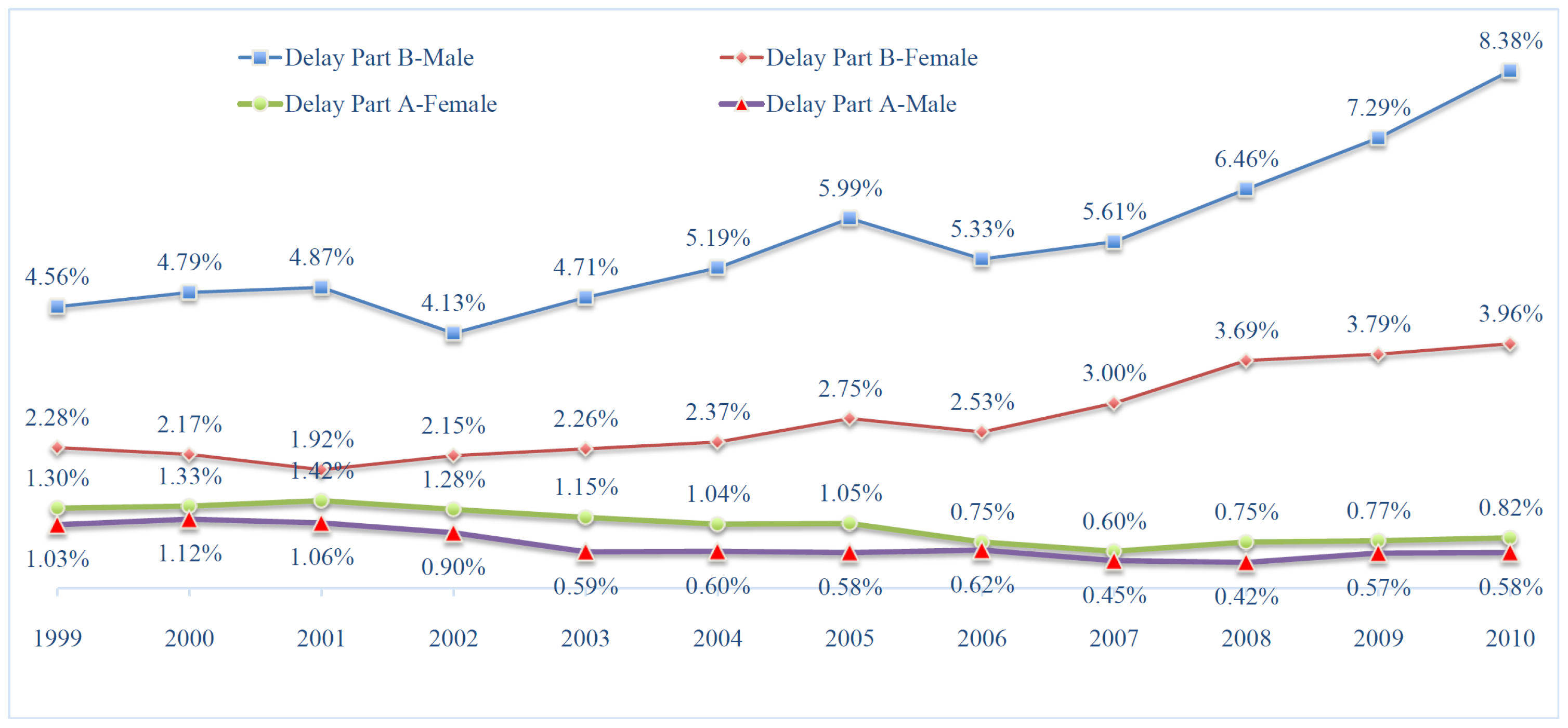
Figure 2.
Annual Medicare cost savings from working. This figure shows the annual Medicare cost savings from working, in billions of dollars, from 1999–2010. The green line (total Medicare savings from working) is the sum of the blue (Medicare savings from more zero Medicare costs) and red (Medicare savings from reduced per person average costs) lines. Authors’ calculation using the estimation results shown in Table 2 and Table 3, and statistics from Table 8.

Figure 3.
Annual Medicare cost savings from MSP. The figure shows the annual Medicare cost savings from MSP, in billions of dollars, from 1999–2010. The green line (total Medicare savings from Medicare as secondary payer) is the sum of the blue (Medicare savings from more zero Medicare costs) and red (Medicare savings from reduced per person average costs) lines. Authors’ calculation using the estimation results shown in Table 2 and Table 3, and statistics from Table 8.

Figure 4.
Annual Medicare cost savings from workers with EPHI. This figure shows the annual Medicare cost savings from workers covered by EPHI, in billions of dollars, from 1999–2010. The green line (total Medicare savings from workers with EPHI) is the sum of the blue (Medicare savings from more zero Medicare costs) and red (Medicare savings from reduced per person average costs) lines. Authors’ calculation using the estimation results shown in Table 2 and Table 3, and statistics from Table 8.

Table 1.
Medical expenditure, by EPHI and working status.
| Not Working | Working | ||||
|---|---|---|---|---|---|
| No EPHI | EPHI | No EPHI | EPHI | ||
| Age = 65∼69, Good Health | |||||
| Medicare Costs | Mean | $3555 | $3245 | $3102 | $1404 |
| S.D. | $8766 | $10,481 | $6943 | $3258 | |
| Total Health Expenditure | Mean | $6444 | $6206 | $5285 | $5503 |
| S.D. | $11,551 | $11,925 | $8367 | $9722 | |
| OOP Expenditure | Mean | $1425 | $1157 | $1285 | $1412 |
| S.D. | $3127 | $2049 | $2079 | $2094 | |
| Age = 65∼69, Bad Health | |||||
| Medicare Costs | Mean | $12,504 | $6250 | $8778 | $2598 |
| S.D. | $27,167 | $11,820 | $19,570 | $3240 | |
| Total Health Expenditure | Mean | $17,095 | $12,481 | $11,236 | $12,976 |
| S.D. | $37,580 | $19,018 | $21,540 | $36,894 | |
| OOP Expenditure | Mean | $1939 | $1806 | $2224 | $3048 |
| S.D. | $2987 | $2739 | $5672 | $11,051 | |
Note: Authors’ calculation using data from the pooled 1999–2010 MCBS Cost and Use files, using cross-sectional sample weights.
Table 2.
Regressions of probability of positive medical spending on work and EPHI.
| Variables | Medicare Costs | Total Health Expenditure | OOP Expenditure |
|---|---|---|---|
| (1) | (2) | (3) | |
| Work | −0.055 | 0.001 | 0.000 |
| (0.005) | (0.002) | (0.002) | |
| EPHI | −0.075 | −0.001 | 0.004 |
| (0.014) | (0.005) | (0.007) | |
| wepc | −0.080 | 0.001 | −0.002 |
| (0.017) | (0.007) | (0.009) | |
| Pseudo R | 0.146 | 0.243 | 0.212 |
| Obs. | 95,146 | 95,103 | 95,146 |
Note: Authors’ calculation using data from the pooled 1999–2010 MCBS Cost and Use files. Each column displays the results from a separate regression. All regressions also contain: ghost indicator, age, age squared, health controls, gender, smoking indicators, number of kids, income-level dummies, race, education, marital status, census region dummies, and DRC dummies (see Appendix A Table A3). Robust standard errors, clustered at the individual level, are in parentheses.
Table 3.
Regressions of level of medical spending on work and EPHI.
| Variables | Medicare Costs | Total Health Expenditure | OOP Expenditure |
|---|---|---|---|
| (1) | (2) | (3) | |
| Work | −0.076 | −0.116 | 0.046 |
| (0.021) | (0.021) | (0.013) | |
| EPHI | −0.108 | 0.074 | 0.006 |
| (0.055) | (0.057) | (0.036) | |
| wepc | −0.281 | 0.006 | −0.024 |
| (0.076) | (0.074) | (0.046) | |
| Lambda | −0.806 | −1.871 | −0.364 |
| (0.058) | (0.134) | (0.084) | |
| Wald | 11,934 | 6548 | 7662 |
| p value | 0.000 | 0.000 | 0.000 |
| Obs. | 78,827 | 93,499 | 92,417 |
Note: Authors’ calculation using data from the pooled 1999–2010 MCBS Cost and Use files. Each column displays the results from a separate regression. All regressions also contain: ghost indicator, age, age squared, health controls, gender, smoking indicators, number of kids, income-level dummies, race, education, marital status, and census region dummies (see Appendix A Table A4). Standard errors are in parentheses.
Table 4.
Regressions of level of medical spending on current delayed enrollment.
| (1) With Health Controls | (2) Without Health Controls | |||||
|---|---|---|---|---|---|---|
| Medicare | Total | OOP | Medicare | Total | OOP | |
| Work | −0.102 | −0.106 | 0.051 | −0.146 | −0.135 | 0.035 |
| (0.020) | (0.021) | (0.013) | (0.021) | (0.021) | (0.013) | |
| EPHI | −0.194 | 0.089 | 0.017 | −0.191 | 0.086 | 0.014 |
| (0.055) | (0.056) | (0.036) | (0.055) | (0.059) | (0.036) | |
| wepc | −0.415 | 0.036 | −0.007 | −0.396 | 0.054 | 0.004 |
| (0.076) | (0.073) | (0.047) | (0.076) | (0.077) | (0.047) | |
| Delay–A–current | −0.238 | −0.135 | −1.071 | −0.193 | −0.114 | −1.058 |
| (0.061) | (0.066) | (0.049) | (0.062) | (0.069) | (0.049) | |
| Delay–B–current | 1.144 | −0.369 | −0.285 | 1.108 | −0.366 | −0.286 |
| (0.119) | (0.045) | (0.030) | (0.121) | (0.047) | (0.030) | |
| EPHI–B–current | −0.399 | 0.144 | 0.127 | −0.431 | 0.145 | 0.129 |
| (0.274) | (0.090) | (0.059) | (0.279) | (0.095) | (0.059) | |
| Lambda | −0.722 | −1.813 | −0.378 | −0.664 | −1.895 | −0.378 |
| (0.054) | (0.127) | (0.081) | (0.055) | (0.136) | (0.082) | |
| Wald | 14,235 | 7073 | 8028 | 12,986 | 5966 | 7692 |
| p value | 0.000 | 0.000 | 0.000 | 0.000 | 0.000 | 0.000 |
| Obs. | 78,827 | 93,499 | 92,417 | 78,827 | 93,499 | 92,417 |
Note: Authors’ calculation using data from the pooled 1999–2010 MCBS Cost and Use files. Each column displays the results from a separate regression. All regressions shown also contain (but are not reported in the table): ghost indicator, age, age squared, health controls, smoking indicators, number of kids, income-level dummies, race, education, marital status, and census region dummies. Standard errors are in parentheses.
Table 5.
Regressions of level of medical spending on current and past delayed enrollment.
| (1) With Health Controls | (2) Without Health Controls | |||||
|---|---|---|---|---|---|---|
| Medicare | Total | OOP | Medicare | Total | OOP | |
| Work | −0.102 | −0.106 | 0.057 | −0.146 | −0.135 | 0.042 |
| (0.020) | (0.020) | (0.015) | (0.021) | (0.021) | (0.015) | |
| EPHI | −0.194 | 0.089 | 0.068 | −0.191 | 0.086 | 0.065 |
| (0.055) | (0.056) | (0.041) | (0.055) | (0.059) | (0.042) | |
| wepc | −0.415 | 0.036 | −0.036 | −0.396 | 0.054 | −0.026 |
| (0.076) | (0.073) | (0.054) | (0.076) | (0.077) | (0.054) | |
| Delay–A–current | −0.236 | −0.132 | −1.760 | −0.190 | −0.111 | −1.748 |
| (0.061) | (0.066) | (0.049) | (0.062) | (0.069) | (0.049) | |
| Delay–B–current | 1.145 | −0.368 | −0.218 | 1.110 | −0.365 | −0.215 |
| (0.119) | (0.045) | (0.034) | (0.121) | (0.047) | (0.034) | |
| EPHI–B–current | −0.399 | 0.143 | 0.062 | −0.432 | 0.144 | 0.062 |
| (0.274) | (0.090) | (0.067) | (0.279) | (0.094) | (0.068) | |
| Delay–past | 0.025 | 0.035 | −0.201 | 0.027 | 0.036 | −0.196 |
| (0.036) | (0.039) | (0.029) | (0.037) | (0.040) | (0.029) | |
| Lambda | −0.722 | −1.811 | −1.176 | −0.664 | −1.894 | −1.221 |
| (0.054) | (0.127) | (0.096) | (0.055) | (0.136) | (0.098) | |
| Wald | 14,235 | 7099 | 12,482 | 12,986 | 5981 | 12,064 |
| p value | 0.000 | 0.000 | 0.000 | 0.000 | 0.000 | 0.000 |
| Obs. | 78,827 | 93,499 | 93,499 | 78,827 | 93,499 | 93,499 |
Note: Authors’ calculation using data from the pooled 1999–2010 MCBS Cost and Use files. Each column displays the results from a separate regression. All regressions shown also contain (but are not reported in the table): ghost indicator, age, age squared, health controls, smoking indicators, number of kids, income-level dummies, race, education, marital status, and census region dummies. Standard errors are in parentheses.
Table 6.
Results from multiple model specifications on Medicare costs.
| OLS | FE | TPM | Sample Selection | |
|---|---|---|---|---|
| (1) | (2) | (3) | (4) | |
| Work | −0.539 | −0.244 | −0.133 | −0.076 |
| (0.046) | (0.047) | (0.023) | (0.021) | |
| EPHI | −0.735 | −0.176 | −0.189 | −0.108 |
| (0.131) | (0.096) | (0.067) | (0.055) | |
| wepc | −1.153 | 0.081 | −0.419 | −0.281 |
| (0.168) | (0.141) | (0.093) | (0.076) | |
| Lambda | −0.806 | |||
| (0.058) | ||||
| R | 0.217 | 0.061 | 0.195 | |
| Wald | 7662 | |||
| p value | 0.000 | |||
| Obs. | 95,146 | 80,995 | 78,827 | 78,827 |
Note: Authors’ calculation using data from the pooled 1999–2010 MCBS Cost and Use files. The DRC dummies are only included in the OLS specification (they drop from the FE specification), since they are exclusion restrictions in the first stage of the TPM, and the Heckman’s sample selection specifications. All regressions also contain (though they are not reported in the table): age, age squared, gender, smoking indicators, number of kids, income dummies, health controls, race, education, marital status, and census region dummies. Robust standard errors, clustered at the individual level, are in parentheses (expect for sample selection model shown in column (4)).
Table 7.
Results from multiple IV specifications on Medicare costs.
| IV_1 | IV_2 | IV_3 | IV_4 | IV_5 | |
|---|---|---|---|---|---|
| (1) | (2) | (3) | (4) | (5) | |
| Work | −1.208 | −1.403 | −1.394 | −0.817 | −0.906 |
| (0.625) | (0.638) | (0.656) | (0.649) | (0.382) | |
| EPHI | −0.905 | −0.819 | −0.786 | −1.034 | 1.579 |
| (0.280) | (0.285) | (0.292) | (0.289) | (2.860) | |
| F Stat. | 126.979 | 123.102 | 119.706 | 120.686 | 22.920 |
| J test | 0.652 | 3.659 | 1.250 | 55.996 | 0.818 |
| p value_J test | 0.419 | 0.055 | 0.264 | 0.000 | 0.366 |
| Hausman test | 1.189 | 1.892 | 1.772 | 0.201 | 1.004 |
| p value_Hausman test | 0.276 | 0.168 | 0.183 | 0.654 | 0.316 |
| Centered R | 0.195 | 0.194 | 0.171 | 0.177 | 0.178 |
| Obs. | 95,146 | 95,146 | 95,146 | 95,146 | 95,146 |
Note: Authors’ calculation using data from the pooled 1999–2010 MCBS Cost and Use files. The first stage of the IV specifications also includes the exclusion restrictions discussed in the text: whether an individual is married and whether an individual acquired some college education in IV_1, whether an individual is married and number of kids in IV_2, whether an individual is married and DRC35 indicator in IV_3, whether an individual is married and DRC65 indicator in IV_4, and whether an individual is married and whether an individual acquired some college education in IV_5. All regressions also contain (though not reported in the table): age, age squared, gender, smoking indicators, income dummies, health controls, race, and census region dummies. Robust standard errors, clustered at the individual level, are in parentheses.
Table 8.
Weighted population (in millions) of workers and those with EPHI coverage.
| Year | 2004 | 2006 | 2007 | 2008 | 2009 | 2010 |
|---|---|---|---|---|---|---|
| Workers | 4.48 | 4.67 | 4.82 | 5.03 | 5.22 | 5.61 |
| Medicare ≻ 0 | 63.54% | 76.13% | 77.65% | 75.67% | 73.96% | 69.47% |
| Medicare = 0 | 36.46% | 23.87% | 22.35% | 24.33% | 26.04% | 30.53% |
| Prob(Medicare ≻ 0) | 68.17% | 81.67% | 83.31% | 81.18% | 79.34% | 74.53% |
| Diff of Prob. | 4.63% | 5.55% | 5.66% | 5.51% | 5.39% | 5.06% |
| EPHI | 1.22 | 1.29 | 1.37 | 1.27 | 1.30 | 1.64 |
| Medicare ≻ 0 | 60.06% | 62.26% | 60.95% | 60.51% | 62.00% | 47.85% |
| Medicare = 0 | 39.94% | 37.74% | 39.05% | 39.49% | 38.00% | 52.15% |
| Prob(Medicare ≻ 0) | 66.19% | 68.61% | 67.17% | 66.69% | 68.33% | 52.73% |
| Diff of Prob. | 6.13% | 6.35% | 6.22% | 6.18% | 6.33% | 4.88% |
| Workers with EPHI | 0.79 | 0.87 | 0.91 | 0.89 | 0.88 | 1.14 |
| Medicare ≻ 0 | 46.14% | 55.83% | 51.41% | 51.91% | 52.92% | 38.59% |
| Medicare = 0 | 53.86% | 44.17% | 48.59% | 48.09% | 47.08% | 61.41% |
| Prob(Medicare ≻ 0) | 51.20% | 61.95% | 57.04% | 57.60% | 58.72% | 42.82% |
| Diff of Prob. | 5.06% | 6.12% | 5.64% | 5.69% | 5.80% | 4.23% |
| Avg. Medicare Costs | $7291 | $7159 | $7253 | $7007 | $6702 | $6673 |
| Medicare Beneficiaries | 29.70 | 30.14 | 30.87 | 31.93 | 32.81 | 33.90 |
Note: Authors’ calculation using data from the pooled 1999–2010 MCBS Cost and Use files, using cross-sectional sample weights. This table shows the weighted population (in millions) of workers, the weighted population of people covered by EPHI, and the weighted population of workers covered by EPHI in selected years. Average Medicare costs are over the estimation sample in which has positive Medicare costs in a given year.
Table 9.
Annual Medicare cost savings from delay enrollment: retrospective counting.
| Year | Part A | Part B | Part A + B | Total |
|---|---|---|---|---|
| 1999 | 2,508,887,296 | 4,243,138,048 | 4,660,755,456 | 11,412,780,800 |
| 2000 | 2,313,744,384 | 4,583,156,736 | 4,340,261,888 | 11,237,163,008 |
| 2001 | 2,538,497,280 | 4,899,589,120 | 4,858,211,840 | 12,296,298,240 |
| 2002 | 2,320,211,200 | 5,201,255,936 | 4,854,670,848 | 12,376,137,984 |
| 2003 | 1,979,582,976 | 5,410,360,320 | 3,875,293,696 | 11,265,236,992 |
| 2004 | 1,730,988,416 | 5,908,411,392 | 2,985,637,376 | 10,625,037,184 |
| 2005 | 1,316,721,792 | 5,755,548,160 | 1,963,387,648 | 9,035,657,600 |
| 2006 | 1,126,692,480 | 5,247,505,920 | 1,758,030,592 | 8,132,228,992 |
| 2007 | 995,435,840 | 5,421,378,560 | 1,044,982,144 | 7,461,796,544 |
| 2008 | 806,216,000 | 5,601,479,680 | 371,533,472 | 6,779,229,152 |
| 2009 | 488,684,576 | 4,304,261,120 | 184,595,936 | 4,977,541,632 |
Publisher’s Note: MDPI stays neutral with regard to jurisdictional claims in published maps and institutional affiliations. |
© 2021 by the authors. Licensee MDPI, Basel, Switzerland. This article is an open access article distributed under the terms and conditions of the Creative Commons Attribution (CC BY) license (https://creativecommons.org/licenses/by/4.0/).
Share and Cite
MDPI and ACS Style
Deng, Y.; Benítez-Silva, H. An Empirical Model of Medicare Costs: The Role of Health Insurance, Employment, and Delays in Medicare Enrollment. Econometrics 2021, 9, 25. https://0-doi-org.brum.beds.ac.uk/10.3390/econometrics9020025
AMA Style
Deng Y, Benítez-Silva H. An Empirical Model of Medicare Costs: The Role of Health Insurance, Employment, and Delays in Medicare Enrollment. Econometrics. 2021; 9(2):25. https://0-doi-org.brum.beds.ac.uk/10.3390/econometrics9020025
Chicago/Turabian StyleDeng, Yuanyuan, and Hugo Benítez-Silva. 2021. "An Empirical Model of Medicare Costs: The Role of Health Insurance, Employment, and Delays in Medicare Enrollment" Econometrics 9, no. 2: 25. https://0-doi-org.brum.beds.ac.uk/10.3390/econometrics9020025
Note that from the first issue of 2016, this journal uses article numbers instead of page numbers. See further details here.