Climate Finance: Mapping Air Pollution and Finance Market in Time Series

Abstract

Climate finance is growing popular in addressing challenges of climate change because it controls the funding and resources to emission entities and promotes green manufacturing. In this study, we determined that PM${}_{2.5}$, PM${}_{10}$, SO${}_2$, NO${}_2$, CO, and O${}_3$ are the target pollutant in the atmosphere and we use a deep neural network to enhance the regression analysis in order to investigate the relationship between air pollution and stock prices of the targeted manufacturer. We also conduct time series analysis based on air pollution and heavy industry manufacturing in China, as the country is facing serious air pollution problems. Our study uses Convolutional-Long Short Term Memory in 2 Dimension (ConvLSTM2D) to extract the features from air pollution and enhance the time series regression in the financial market. The main contribution in our paper is discovering a feature term that impacts the stock price in the financial market, particularly for the companies that are highly impacted by the local environment. We offer a higher accurate model than the traditional time series in the stock price prediction by considering the environmental factor. The experimental results suggest that there is a negative linear relationship between air pollution and the stock market, which demonstrates that air pollution has a negative effect on the financial market. It promotes the manufacturer’s improving their emission recycling and encourages them to invest in green manufacture—otherwise, the drop in stock price will impact the company funding process.

1. Introduction

Growing industrialization bring serious air pollution in emerging economic entities such as China and India. Paris Climate Accords were signed by 196 parties around the world in order to control the rapid exacerbation of climate change. The concentration of carbon dioxide in Earth’s atmosphere is rapidly rising and is more than 420 parts per million (ppm) according to NASA data. This requires significant action to contain the atmospheric carbon dioxide, which benefits humanity as a whole. Climate finance is a popular topic in recent years, particularly after Paris Climate Accord was signed Bodansky (2016). By utilizing the flexibility of the financial market, resources can be re-allocated to promote the green industry and also offer more funding to traditional manufacturers to improve emission recycling Buchner et al. (2019); Hong et al. (2020). Air pollution plays an important role in the area of climate finance because it determines the concentration of carbon dioxide in the Earth’s atmosphere; carbon dioxide and other pollutants block off the interaction between ultraviolet rays and photosynthesis, which exacerbate global warming Kelp et al. (2018). Emerging economic entities such as China and India are experiencing rapid industrialization, but polluted air is the price they pay for the fast economic growth Anwar et al. (2021). Containing global warming and decreasing air pollution are the responsibility of those countries and of all human beings Lelieveld et al. (2015).

There are a limited number of research studies in modeling the stock prices by climate condition today, and few research outputs are mapping the relationship between the climate condition and financial market today. Air pollution seems far away from the stock market today, but it will have a closer relationship in the near future, as responsible investors are more concerned about long-term returns in their investment, so discovering the relationship between air pollution and the financial market is becoming more and more popular over time Banga (2019). Traditionally, stock prices in the financial market usually depend on the economic condition, revenues of the specific firms, dividend policy Banerjee et al. (2007), and the prospect of the industry Mehtab (2020). Air pollution or the climate condition is less significant as evidence of the hypothesis for the regression analysis. In the meantime, investors or academic researchers are analyzing the time-series pattern of stock prices using lagged value or past volatility by using mathematicak tools such as Stochastic calculus Grigoriu (2013), random processes, ARIMA time series regression Adebiyi et al. (2014), and GARCH volatility model Alberg et al. (2008). However, with the increase in communication efficiency in the market and globalization, the value of financial assets is impacted by various elements, which increasingly depend on factors in both finance and non-finance areas. This means the traditional model is not adequte to analyze all of these features. With the development of computer technology and deep neural networks Pang et al. (2020), people tend to use a more complex model to capture the information that affects the volatility of stock price; long short-term memory (LSTM) is one of the popular deep neural networks used to capture the time series pattern, and the model remembers more long-term information than the recent value Hochreiter and Schmidhuber (1997). On the other hand, convolutional neural networks (CNNs) are widely used in image analysis because they are able to extract the features in the image and capture local dependencies Albawi et al. (2017). Machine learning helps market investors to predict the stock price more accurately than the traditional model and have better forecasting on the future market volatility. There is also a combination deep neural network model that includes CNN and LSTM together, called ConvLSTM2D Sari et al. (2020), which has been widely used in video classification because the convolutional layers are able to capture the information in each picture of video and LSTM provides the long term memory, the model can remember information in the past few seconds in the video.

The price of financial assets will be more reliant on the climate condition particularly after the Paris Climate Agreement, and large globalized organizations are pushing for decarbonization. In this paper, we propose a novel structure in regression and neural network technique to model the stock price and environmental factor in order to provide a more accurate time series model in stock price and offer a sustainability view to investors in targeted companies. We modeling the stock price based on the traditional time series model and the deep neural network ConvLSTM2D and use it to enhance the time series regression in predicting the stock price. Our model includes the autoregressive model (AR) and the feature term we call $A{P}_1$, which contains the information extracted by the ConvLSTM2D from the air pollution data. The experiments use the air pollution data from the four major industrialized cities in China, which are Beijing, Taiyuan, Changchun, and Shijiazhuang. We take the sample of the concentration of PM${}_{2.5}$, PM${}_{10}$, SO${}_2$, NO${}_2$, CO, and O${}_3$ in the atmosphere to indicate the air pollution from 1 January 2015 to 31 October 2021. The initial value of $A{P}_1$ is the mean of scaled air pollution data, which uses back-propagation and gradient descent to update the value of $A{P}_1$ in the regression model and then re-trained by the deep neural network model again.. By utilizing the advantage of ConvLSTM2D, the local dependencies and long-term dependencies in air pollution will be measured and captured by the model, and updating the regression in stock price models all this information together. The aim of our paper is to provide an accurate model to capture information from air pollution and time-series patterns, which demonstrates the relationship between the stock price and climate conditions. The samples of the stock price taken in this paper are several top capitalization manufacturers in China, and those companies have large size of factories located in those selected cities, which include Shougang Group, Shenhua Group, Sany Group from Beijing. Datong Coal Mining, Shanxi Coal International, and Sanxi Coking Co from Taiyuan, as well as Hbis Group and Maanshan Iron & Steel from Shijiazhuang. FAW Jiefang and FAWAY from Changchun.

The rest of this paper is organized as follows. Section 2 demonstrates the related background of the traditional time series model and the model selection techniques. Section 3 introduces the background of ConvLSTM2D and outlines the methodology of this paper by combining the traditional model with the deep neural network. Section 4 describes an experimental study to demonstrate the relationship between air pollution and stock price. Section 5 concludes the findings and demonstrates the future development of climate finance and green manufacturing.

2. Time Series Modeling

This section introduces the related background of time series analysis based on Box–Jenkins’s theory Box et al. (2015, 1976).

2.1. Box–Jenkins’s Method

The autoregressive integrated moving average (ARIMA) model is widely used in the current time series modeling, and it takes the lag value of the timestamp in time series and regression error, which is a linear combination of error terms. ARIMA is a general form of Autoregressive-Moving Average (ARMA) that adds the differencing order for the value of each timestamp. The ARIMA model takes the parameters of $(p,d,q)$, represented as the lag order of p in the Autoregressive (AR) model, the lag order of q in the Moving Average (MA) model, and the $dth$ differencing order Box et al. (2015, 1976). The formula of ARMA$(p,q)$ model is:

$$X_t=c+\sum _{i=1}^p{\varphi }_i{X}_{t-i}+{ϵ}_t+\sum _{i=1}^q{\theta }_i{ϵ}_{t-i}$$

(1)

where $\left\{{ϵ}_t\right\}\sim WN(0,{\sigma }^2).$

The particular case of ARMA with integer order of differencing usually used to process the time series value to be stationery, using B to represent the backshift operator Box et al. (2016) and then the ARIMA$(p,d,q)$ can be rewritten as:

$$(1-\sum _{i=1}^p{\varphi }_i{B}^i){(1-B)}^d{X}_t=(1+\sum _{i=1}^q{\theta }_i{B}^i){ϵ}_t$$

(2)

The ARIMA model gives the user flexibility to decide the parameters; if setting $q=0,d=0$, the ARIMA modeling is the same as that of the autoregressive model. In the experiment part of this paper, we use the autoregressive model with a linear combination of lag values of current timestamp and feature term $A{P}_1$, given as:

$$X_t=c+\sum _{i=1}^p{\varphi }_i{X}_{t-i}+A{P}_1$$

(3)

The likelihood function for the autoregressive model assuming the data generated from a mean zero $\mu =0$ stationary AR$\left(p\right)$ with Gaussian error. Suppose there is a sample of N observation $y=(y_1,\dots ,y_n)$ with $c=0$ and denote the parameter vector $\beta =({\varphi }_1,\dots ,{\varphi }_p,{\sigma }^2)$ Fang et al. (2021a, 2021b), the corresponding unconditional log-likelihood function is given as:

$$L\left(y\beta \right)=-\frac{N}{2}log\left(2\pi {\sigma }^2\right)-\frac{1}{2}log\Sigma -\frac{1}{2{\sigma }^2}{y}^T{\Sigma }^{-1}y$$

(4)

where $\Sigma$ is the determinant of $\Sigma$ and ${\sigma }^2\Sigma$ is the $N\times N$ theoretical autocovariance matrix of $y.$

2.2. Model Selection

Model selection techniques are used to determine the parameter for the model; there are popular model selections from information-theoretic studies, such as Akaike’s Information Criterion (AIC) Akaike (1974); Sakamoto et al. (1986), Bayesian Information Criterion (BIC) Neath and Cavanaugh (2012), and Hannan–Quinn (HQ) Bierens (2004), given as:

• AIC = $log\left(L\right)+\frac{2(p+k+1)}{N}$.
• BIC = $log\left(L\right)+\frac{(p+k+1)log\left(L\right)}{N}$
• HQ = $log\left(L\right)+\frac{2(p+k+1)loglogN}{N}$

where $k=1$ if intercept $c\ne 0$ and $k=0$ if intercept $c=0$, N is the number of observations for a given time series, and L is likelihood of the data.

In this paper, we use the new Bayesian information criteria for selecting the parameters in AR$\left(p\right)$, which is Minimum Message Length (MML). It has been proven to work well in the time series analysis including AR Fitzgibbon et al. (2004), MA Sak et al. (2005), and ARMA model Fang et al. (2021b), MML was introduced by Wallace and Freeman. MML is based on coding theory and assumes the sender transmits the message to the receiver; its methodology is to encode a two-part message, where the first part is the time series model and the second part is data in the given model. The receiver decodes the message by using Bayesian prior. MML thus gives a quantitative information-theoretic trade-off between model complexity (length of the first part of the message) and goodness of fit (length of the second part of the message) and selects the parameter with a minimum value of MML.

The formula of MML is

$$MessLen(\beta ,y)=-log\left(\frac{\pi \left(\beta \right)f(y_1,\dots ,y_n\beta ){ϵ}^n}{\sqrt{F\left(\beta \right)}}\right)+\frac{k}{2}(1+log{\kappa }_k)-logh\left(k\right)$$

(5)

where $\pi \left(\beta \right)$ is the Bayesian prior distribution over the parameter set and $f(y_1,\dots ,y_n\beta )$ is likelihood function from equation from (4). ${ϵ}^n$ is an indication of accuracy of data, $F\left(\beta \right)$ is the Fisher Information matrix of the parameter vector $\beta$, which plays an essential role in MML. $h\left(k\right)$ is the prior on parameter p. ${\kappa }_k$ is the lattice constant where k is number of free parameters; it is bounded above by $\frac{1}{12}$ and bounded below by $\frac{1}{2\pi e}$, accounting for the expected error in log-likelihood function autoregressive model given in Equation (4). According to the papers Fang et al. (2021a, 2021b), MML works well in the traditional time series modeling and hybrid model with the neural network.

3. Methodology and Data

3.1. Methodology

ConvLSTM2D maps the convolutional neural network (CNN) with the LSTM model, as the ConvLSTM2D treats the convolutional layer as the value in each timestamp and utilizes LSTM in the time series analysis. Liu et al. (2017) demonstrated that Conv-LSTM is a highly accurate deep learning model in short-term forecasting through the se of traffic data, and outperforms the traditional ARIMA model or LSTM. By utilizing the advantages of LSTM and CNN, ConvLSTM2D is able to memory the long=term information for the convolutional layer, and Xu also show that the ConvLSTM structure works well in air pollution prediction Xu and Lv (2019). Retta and Kethavath (2021) previously showed that CNN-RNN works well in air pollution forecasting, particularly for PM${}_{2.5}$. CNN is widely used in image classification as it extracts pixel information by the kernel or filter with the proper level of strides; kernels usually have three channels for colorful images (RGB). By setting the appropriate size of the kernel, CNN maps the pixel into the next convolution layer after the matrix multiplication, so the information in the image is projected to the next layer and carried forward Albawi et al. (2017). There is usually more than one kernel used to scan the images and extract different information. The activation function of ReLU (6) Agarap (2018) and Sigmoid (7) Yonaba et al. (2010) are popularly used in the classification task. The ConvLSTM2D inputs the two-dimensional matrix values in the convolutional neural network and continues to train with the LSTM model by flattening the CNN output, and the final step uses a fully connected dense layer to conduct the classification or regression tasks.

$$ReLU=max(0,x)$$

(6)

$$Sigmoid=\sigma \left(x\right)=\frac{1}{1+e^{-x}}$$

(7)

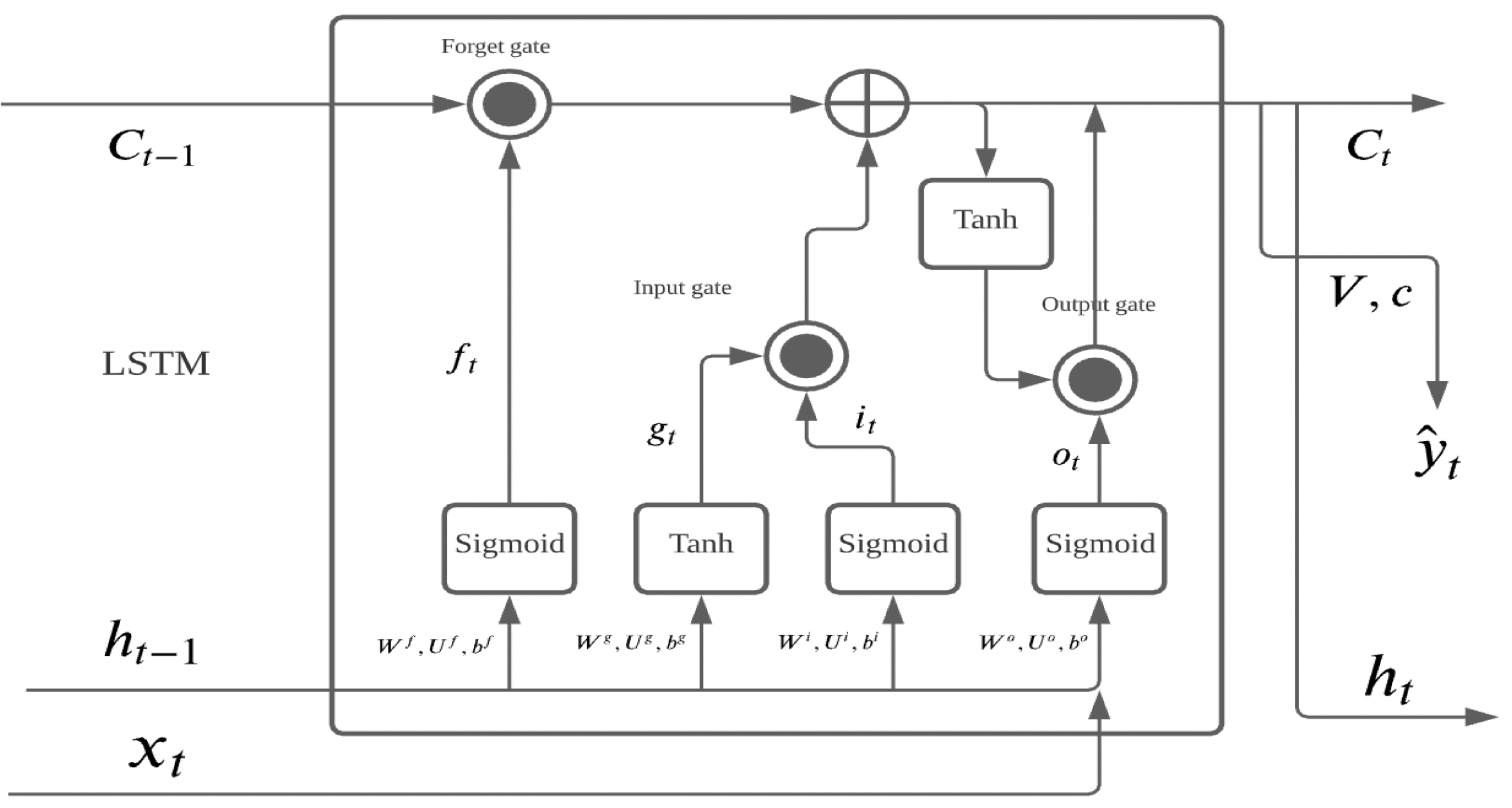
Figure 1 shows the architecture of the LSTM, as it maintains an information highway from $C_{t-1}$ to $C_t$ to allow the model to use memory from past information Hochreiter and Schmidhuber (1997). The LSTM uses a gate mechanism, including input gate, forget gate, and output gate, to determine how much information should be carried forward from this layer to the next layer by using the element-wise operation from the sigmoid activation function of the input. If the output from the sigmoid activation function is closer to 0, it indicates the large proportion of information should be forgotten; otherwise, the current layer will carry more information into the next layer and the model will be trained by back-propagation.

The LSTM employ the following operation:

• $g_t$ = $tanh(W^g{h}_{t-1}+U^g{x}_t+b^g)$
• Forget gate: $f_t=\sigma (U^f{x}_t+W^f{h}_{t-1}+b^f)$
• Input gate: $i_t=\sigma (U^i{x}_t+W^i{h}_{t-1}+b^i)$
• Long-term state: $c_t=f_t\odot c_{t-1}+g_t\odot i_t$
• Output gate: $o_t=\sigma (U^o{x}_t+W^o{h}_{t-1}+b^o)$
• Short-term state: $h_t=o_t\odot tanh\left(c_t\right)$
• Output: ${\widehat{y}}_t=V{h}_t+c$

where W and U are parameters for the information from the previous hidden state and current hidden state, b is the bias term, and V is the parameter of output.

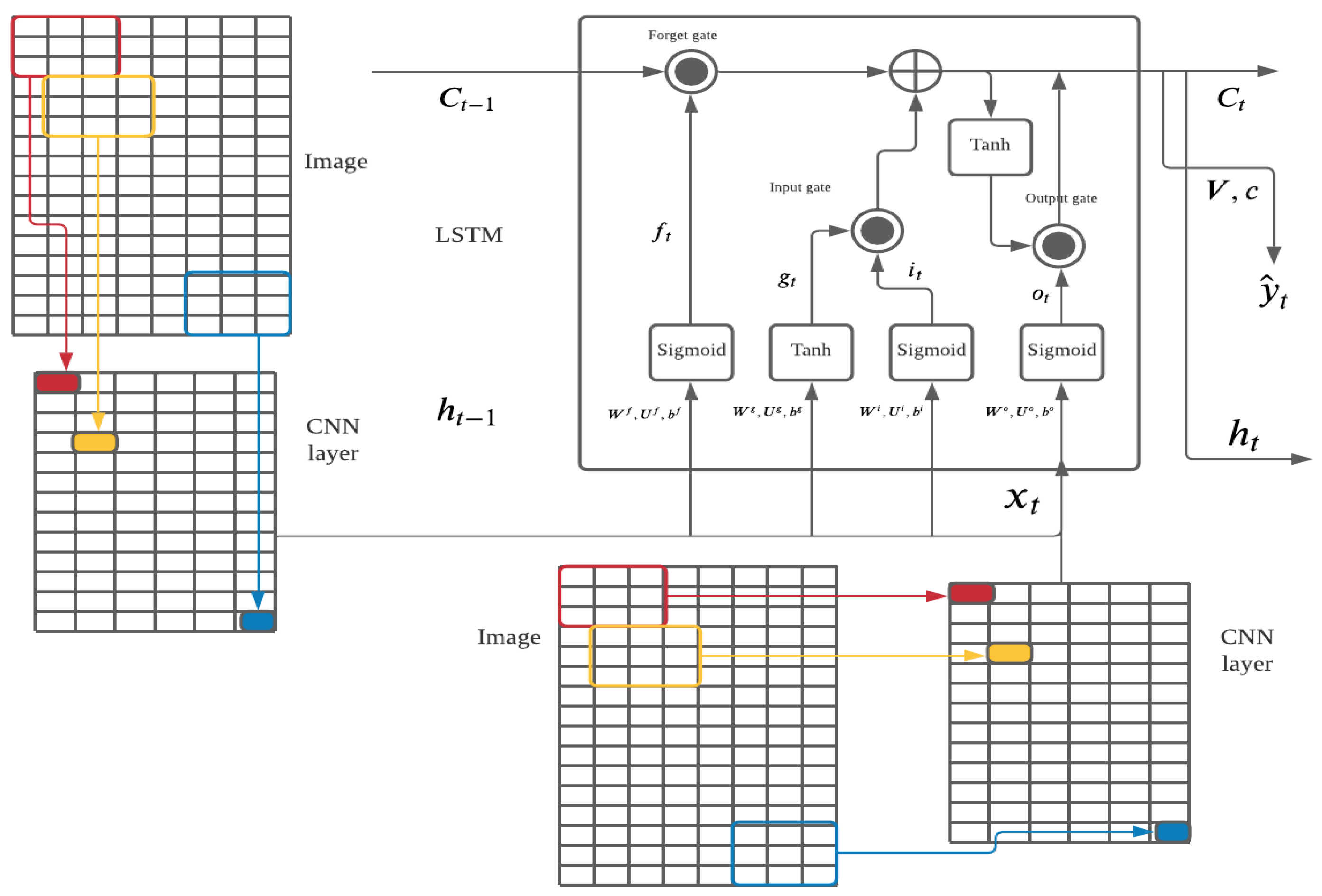
The $X_t$ is the input vector for the time series value in LSTM; however, the $X_t$ will take the convolutional layer as input in the ConvLSTM2D model, the architecture of ConvLSTM2D shown in Figure 2. The ConvLSTM structure has been suggested to work well in the stock market prediction because of extracting the local dependencies with the time series pattern based on Kelotra’s paper Kelotra and Pandey (2020).

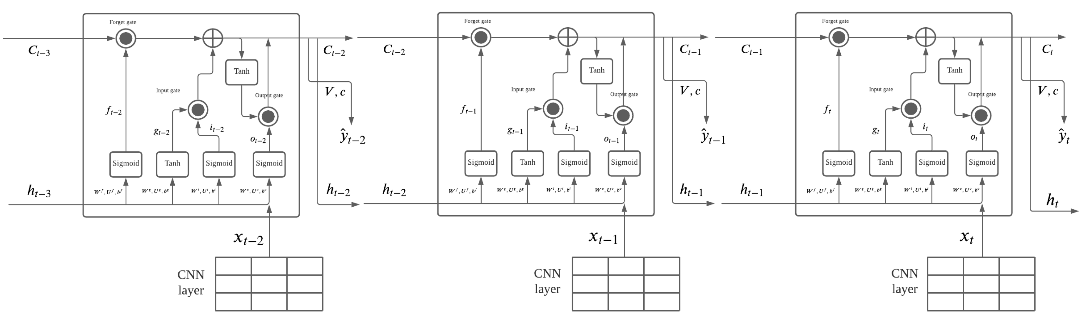
Overlapping each LSTM layer together to form the whole architecture of ConvLSTM2D, it provides the convolutional layers with a time series characteristic and creates a model that captures long-term and short-term dependencies, as shown in Figure 3.

We use ConvLSTM2D to capture air pollution information. There are local dependencies between the air pollutants PM${}_{2.5}$, PM${}_{10}$, SO${}_2$, NO${}_2$, CO, and O${}_3$, because the manufacturer usually emits continuous emissions with the admixture of different pollutants. In the meantime, the pollutants will not disperse in the atmosphere in a short amount of time and will stay to impact air quality in the coming days. Using the convolutional neural network will enable capturing the local dependencies in those pollutants each day, and treating them as the input of LSTM to capture the long-term and short-term patterns in time series. To address the challenge of modeling the relationship between air pollution condition and stock price, we initialize the feature term $A{P}_1$ as the scaled mean of different pollutants in the length of days prior to the current stock price $X_t$ as given below:

$$X_t=c+\sum _{i=1}^p{\varphi }_i{X}_{t-i}+A{P}_1$$

(8)

The parameter of p is determined by the Minimum Message Length (MML) from Equation (5) in Section 2.2 and uses the ordinary least squares (OLS) from linear regression to model the stock price of $X_t$. In the meantime, the initial value of $A{P}_1$ will be updated by gradient descent in pre-set number of epochs, and back-propagation will enhance the linear relationship between the stock prices and feature term $A{P}_1$. The hybrid model of ConvLSTM2D and Autoregressive provides the time series regression from the lagged value of stock price and feature extracted from the air pollution, and the relationship is expressed by the linear regression. The algorithm and model construction processes shown in the Algorithm 1.

Algorithm 1 Algorithm with ConvLSTM2D Model

Require: number of epochs $=20$ while i ≤ epochs do     model.add(ConvLSTM2D(filters=64, kernel size=(3, 3), input shape=(batch size, number of frames, height, width, channels), padding= “same”, return sequences=True, activation=“relu”))     model.add(BatchNormalization())     model.add(ConvLSTM2D(filters=64, kernel size=(3, 3), padding=“same”, return sequences=True, activation=“relu"))     model.add(Flatten())     model.add(Dense(256, activation=‘relu’))     model.add(Dense(1)) end while

We use the 64 different kernel with size of 2 dimension 3 × 3 and default stride of one and zero padding. The deep neural network ConvLSTM2D is trained by open-source software Tensorflow and Keras that uses the mean squared error (MSE) as the loss function and the optimizer of adam, and the model can learn the best feature term related to the targeted stock price.

Linear regression provides double training for the results from the ConvLSTM2D shown in the Algorithm 2. The hyper-parameter of the learning rate $\eta =0.1$, and the number of epochs $=10$, the loss function used is:

$$J\left(\theta \right)=\frac{1}{2}{(y-\widehat{y})}^2$$

(9)

the gradient regarding with the feature term $A{P}_1$ calculated by chain rule is given as:

$$\frac{\partial J\left(\theta \right)}{\partial A{P}_1}=\frac{\partial J\left(\theta \right)}{\partial \widehat{y}}\frac{\partial \widehat{y}}{\partial A{P}_1}=(y-\widehat{y})\ast W_{A{P}_1}$$

where $W_{A{P}_1}$ is the coefficient for the feature term $A{P}_1$.

Algorithm 2 Algorithm with updating feature term $A{P}_1$ by using gradient descent

Require: number of epochs $=10$  while i ≤ epochs do    1. Predicting the value of feature term $A{P}_1$ from trained ConvLSTM2D model    2. Modeling the linear regression by ordinary least squares    3. Using gradient descent and hyperparameter of learning rate.to update the feature term $A{P}_1$    4. Train ConvLSTM2D model by new feature term $A{P}_1$  end while

3.2. Data

This section demonstrates experimental studies for modeling the air pollution data and stock prices. We select four major industrialized cities in China, namely Beijing, Taiyuan, Changchun, and Shijiazhuang, and also include ten leading heavy manufacturers in China with a high amount of capital. The air pollution data were collected from the Ministry of Ecology And Environment in China, and stock prices were collected from Yahoo Finance. The selected manufacturers have headquarters or main factories located in those cities, so they interact with local environment governments and are impacted by the local air pollution. The selected manufacturers are Shougang Group, Shenhua Group, and Sany Group from Beijing; Datong Coal Mining, Shanxi Coal International, and Sanxi Coking Co from Taiyuan; Hbis Group and Maanshan Iron & Steel from Shijiazhuang; and FAW Jiefang and FAWAY from Changchun. We believe that taking air pollution data into account would increase the performance of predicting the stock prices for the heavy manufacturers.

4. Experiment

To evaluate the performance, we first divided the dataset such that 95% was in the sample and the remaining 5% as out of sample estimation, which included a 54-ahead forecast window, and we conducted a rolling forecast. We compared our model results with ARIMA, which was implemented using the auto.arima() function of the forecast package for R Hyndman et al. (2020) and this function outputs the best ARIMA model by information criteria of AIC and parameters of maximum p and q. Fang previously showed the MML selects the ARIMA model with lower prediction errors than AIC and BIC, and MML also outperforms in selecting the lower RMSE in the hybrid ARIMA-LSTM model Fang et al. (2021a, 2021b).

Table 1. Parameters of p in AR$\left(p\right)$ selected by MML for different stock and learning rate $\eta$ used in different stock.

Parameters of p in AR$\left(\mathit{p}\right)$ Selected by MML for Different Stock and Learning Rate $\mathit{\eta }$ Used in Different Stock
	Beijing			Taiyuan			Shijiazhuang		Changchun
	Shougang	Shenhua	Sany	Datong Coal	Shanxi Coal	Sanxi Coking	Hbis	Maanshan Iron & Steel	FAW Jiefang	FAWAY
p	2	2	2	2	2	3	2	2	3	5
$\eta$	0.001	0.001	0.001	0.1	0.1	0.1	0.01	0.01	0.1	0.1

shows parameters p in our model are selected by MML and learning rate $\eta$ used in ConvLSTM2D. Secondly, we compared the model with the historical mean model of stock price itself. Finally, we conducted a hypothesis test regarding the feature term $A{P}_1$ extracted from prior 30 days of air pollution data to the targeted variable. The initial value of $A{P}_1$ uses a scalar of minimum and maximum values in the range of 0 to 1 and then uses back-propagation to update this value to record the linear dependencies between stock price and air pollution.

4.1. Beijing

We evaluated model performance according to MAE (10), RMSE (11), and SSE (12) Chen et al. (2013); Zhao et al. (2018).

$$MAE=\frac{1}{n}\sum _{i=1}^n{e}_t$$

(10)

$$RMSE=\sqrt{\frac{1}{n}\sum _{i=1}^n{e}_t^2}$$

(11)

$$SSE=\sum _{i=1}^n{e}_t^2$$

(12)

Table 2. Air pollution model comparison for the stock prices predictions of three selected heavy manufacturers in Beijing.

Model Comparison for the Stock Prices of Heavy Manufacturers in Beijing
		MAE	1.667209		MAE	3.225985		MAE	2.147781
Our model	Shougang	RMSE	1.886901	Shenhua	RMSE	3.877564	Sany	RMSE	2.54785
		SSE	192.2613		SSE	811.9173		SSE	350.5432
		MAE	1.910572		MAE	2.660931		MAE	2.502593
ARIMA	Shougang	RMSE	2.137925	Shenhua	RMSE	3.16369	Sany	RMSE	2.967872
		SSE	246.819		SSE	540.4825		SSE	475.6462
		MAE	2.678831		MAE	6.436293		MAE	14.61221
Historical mean	Shougang	RMSE	2.853079	Shenhua	RMSE	6.844118	Sany	RMSE	14.79293
		SSE	439.5633		SSE	2529.466		SSE	11816.86

shows the performance comparison between different models in three selected stock prices for manufacturers located in Beijing; the results suggest that there is a regression relationship between the air pollution of prior 30 days and the current stock prices in the heavy manufacturing industry. Table 2 suggests that our model has lower prediction errors in terms of MAE, RMSE, and SSE for the selected manufacturers of Shougang and Sany. The linear model combining the feature term $A{P}_1$ better explains the long-term dependencies for the stock price, as it has lower errors, through combining with the short term dependencies of the autoregressive model, which more accurately predicts the stock price.

We tested the hypothesis regarding the significance of the population linear relationship between the feature term $A{P}_1$ and $X_t$. The null hypothesis tests if the population slope is equal to 0, whereas the alternative hypothesis is that the population slope is not equal to 0, based on the econometrics theory of Wooldridge (2015).

$$H_0:W_{A{P}_1}=0$$

$$H_1:W_{A{P}_1}\ne 0$$

According to

Table 3. Linear regression information for the stock prices of heavy manufacturers in Beijing.

Linear Regression Information
		Coefficients	Std. Error	t value	Pr(>t)
	Intercept	0.01068	0.03091	0.345	0.7298
Shougang	$A{P}_1$	0.52152	0.24484	2.130	0.0333
	$la{g}_2$	0.45570	0.02264	20.131	<2$\times {10}^{-16}$
	$la{g}_1$	0.53029	0.02267	23.395	<2$\times {10}^{-16}$
		Coefficients	Std. Error	t value	Pr(>t)
	Intercept	0.29036	0.08952	3.244	0.00121
Shenhua	$A{P}_1$	−1.34605	0.52752	−2.552	0.01082
	$la{g}_2$	0.12063	0.02525	4.777	1.95$\times {10}^{-16}$
	$la{g}_1$	0.86798	0.02526	34.367	<2$\times {10}^{-16}$
		Coefficients	Std. Error	t value	Pr(>t)
	Intercept	0.37402	0.07062	5.296	1.35$\times {10}^{-7}$
Sany	$A{P}_1$	−3.37391	0.63969	−5.274	1.52$\times {10}^{-7}$
	$la{g}_2$	0.02706	0.02532	1.069	0.285
	$la{g}_1$	0.96849	0.02535	38.208	<2$\times {10}^{-16}$

, the p-values for the feature term $A{P}_1$ in the manufacturers Shougang, Shenhua, and Sany are less than 0.05 significance level, where the lower p-value indicates the lower probability of null hypothesis $H_0$ holding true; this also suggests that the alternative hypothesis $H_1$ holds true Biau et al. (2010). We can conclude that the variable feature term $A{P}_1$ is significant in this model and has a relationship with the stock price. Thus, we conclude that there is statistically significant evidence that the independent variables of feature term $A{P}_1$ and dependent variable stock price $X_t$ are linearly related Emmert-Streib and Dehmer (2019). As we can see that the coefficients of feature term $A{P}_1$ are negative in the company of Shenhua and Sany, which indicates the negative linear relationship with the stock price, demonstrating that air pollution has a negative effect on the financial market. This encourages the manufacturer to improve their emission recycling and encourage them to invest in green manufacture to prevent the drop in stock price from impacting the company funding process.

4.2. Taiyuan

Table 4. Comparison of air pollution models for the stock prices predictions of three selected heavy manufacturers in Taiyuan.

Model Comparison for the Stock Prices of Heavy Manufacturers in Taiyuan
		MAE	3.870204		MAE	3.09871		MAE	2.432536
Our model	Datong	RMSE	4.493543	Shanxi	RMSE	3.737073	Sanxi	RMSE	2.984308
		SSE	1090.364		SSE	754.1486		SSE	480.9291
		MAE	3.341736		MAE	2.864032		MAE	2.467751
ARIMA	Datong	RMSE	3.941559	Shanxi	RMSE	3.501327	Sanxi	RMSE	3.004132
		SSE	838.9378		SSE	662.0017		SSE	487.3397
		MAE	5.834804		MAE	5.004533		MAE	3.369719
Historical mean	Datong	RMSE	6.262535	Shanxi	RMSE	5.529563	Sanxi	RMSE	3.838642
		SSE	2117.845		SSE	1651.108		SSE	795.6992

demonstrates the different models’ performance in the manufacturers of Datong Coal Mining, Shanxi Coal International, and Sanxi Coking Co from the city of Taiyuan. The selected companies are the largest coal mining producers in China, which determines the economic growth in the Shanxi province Li et al. (2017).

The results from Table 4 suggest that our model outperforms for the companies of Sanxi in terms of lower forecasting error than ARIMA or historical mean models, and the feature terms $A{P}_1$ have a significant relationship with the stock price. The coal producers are obviously correlated with the air pollution because of the huge amount of PM${}_{2.5}$, PM${}_{10}$, and CO emission into the atmosphere during the mining processes Li and Hu (2017). Taiyuan is the capital city of Shanxi province and the leading producer of coal in China. This province stores one-third of China’s coal deposits Li and Hu (2017). The stock price of coal mining producers and feature term $A{P}_1$ from air pollution show a positive relationship with the large coefficient shown in

Table 5. Linear regression information for the stock prices of heavy manufacturers in Beijing.

Linear Regression Information
		Coefficients	Std. Error	t value	Pr(>t)
	Intercept	−0.21564	0.03424	−6.298	3.92$\times {10}^{-10}$
Datong	$A{P}_1$	1.98953	0.16299	12.207	<2$\times {10}^{-16}$
	$la{g}_5$	−0.08842	0.02430	−3.638	0.00283
	$la{g}_4$	0.11288	0.03054	3.696	0.000227
	$la{g}_3$	0.01822	0.03084	0.591	0.554809
	$la{g}_2$	0.17709	0.03053	5.800	8.03 $\times {10}^{-09}$
	$la{g}_1$	0.75360	0.02432	30.992	<2$\times {10}^{-16}$
		Coefficients	Std. Error	t value	Pr(>t)
	Intercept	−0.96186	0.02383	−40.362	<2$\times {10}^{-16}$
Shanxi	$A{P}_1$	4.93618	0.10239	48.209	<2$\times {10}^{-16}$
	$la{g}_2$	0.16002	0.01605	9.971	<2$\times {10}^{-16}$
	$la{g}_1$	0.83104	0.01605	51.778	<2$\times {10}^{-16}$
		Coefficients	Std. Error	t value	Pr(>t)
	Intercept	−0.41074	0.03359	−12.228	<2$\times {10}^{-16}$
Sanxi	$A{P}_1$	3.42941	0.15495	22.133	<2$\times {10}^{-16}$
	$la{g}_3$	0.12370	0.02206	5.609	2.41$\times {10}^{-08}$
	$la{g}_2$	0.25412	0.02522	10.078	<2$\times {10}^{-16}$
	$la{g}_1$	0.57790	0.02210	26.155	<2$\times {10}^{-16}$

; it is reasonable as coal mining promotes the stock price and increases air pollution at the same time.

4.3. Shijiazhuang

Shijiazhuang is one of the main industrialized cities in north China and has suffered from air pollution in the last decade.

Table 6. Air pollution model comparison for the stock prices predictions of three selected heavy manufacturers in Shijiazhuang.

Model Comparison for the Stock Prices of Heavy Manufacturers in Shijiazhuang
		MAE	0.476300		MAE	1.330529
Our model	Hbis	RMSE	0.532923	Maanshan	RMSE	1.495913
		SSE	15.33638		SSE	120.8388
		MAE	0.516722		MAE	1.596509
ARIMA	Hbis	RMSE	0.571172	Maanshan	RMSE	1.742506
		SSE	17.61684		SSE	163.9617
		MAE	0.225341		MAE	2.35427
Historical mean	Hbis	RMSE	0.257499	Maanshan	RMSE	2.462239
		SSE	3.580536		SSE	327.3815

shows a comparison of models for accuracy in different stock price predictions. It experiment shows that our model outperforms ARIMA and the historical mean model in forecasting. The results suggest that our model has lower MAE, RMSE, and SSE because it maps the air pollution feature projected into regression analysis. The results also indicate long-term dependencies of time series in the manufacturers of heavy industry with respect air, quality as

Table 7. Linear regression information for the stock prices of heavy manufacturers in Shijiazhuang.

Linear Regression Information
		Coefficients	Std. Error	t value	Pr(>t)
	Intercept	0.002514	0.018013	0.140	0.8890
Hbis	$A{P}_1$	0.192569	0.093631	2.057	0.0399
	$la{g}_2$	0.257325	0.024587	10.466	<2$\times {10}^{-16}$
	$la{g}_1$	0.731314	0.024607	29.720	<2$\times {10}^{-16}$
		Coefficients	Std. Error	t value	Pr(>t)
	Intercept	0.023264	0.016088	1.446	0.148
Maanshan	$A{P}_1$	−0.062328	0.538827	2.198	0.0325
	$la{g}_2$	0.004165	0.025510	0.163	0.870
	$la{g}_1$	0.985218	0.025493	38.647	<2$\times {10}^{-16}$

justifies the significance of linear regression between feature term $A{P}_1$ and the targeted variable of stock price because of a lower p-value than the benchmark of 0.05 in the hypothesis test.

4.4. Changchun

The results from

Table 8. Air pollution model comparison for the stock prices predictions of three selected heavy manufacturers in Changchun.

Model Comparison for the Stock Prices of Heavy Manufacturers in Changchun
		MAE	2.107585		MAE	1.227716
Our model	FAW Jiefang	RMSE	2.266491	FAWAY	RMSE	1.426226
		SSE	277.3969		SSE	109.8424
		MAE	5.223868		MAE	0.592963
ARIMA	FAW Jiefang	RMSE	5.270225	FAWAY	RMSE	0.632561
		SSE	1499.864		SSE	21.6072
		MAE	5.746878		MAE	0.738691
Historical mean	FAW Jiefang	RMSE	5.78802	FAWAY	RMSE	0.79334
		SSE	1809.064		SSE	33.987

and

Table 9. Linear regression information for the stock prices of heavy manufacturers in Changchun.

Linear Regression Information
		Coefficients	Std. Error	t value	Pr(>t)
	Intercept	−0.31293	0.03808	−8.218	4.33 $\times {10}^{-15}$
FAW Jiefang	$A{P}_1$	3.81093	0.19918	19.134	<2$\times {10}^{-16}$
	$la{g}_2$	−0.08317	0.02279	−3.649	0.00272
	$la{g}_1$	1.05703	0.02283	46.296	<2$\times {10}^{-16}$
		Coefficients	Std. Error	t value	Pr(>t)
	Intercept	−0.013665	0.038441	−0.355	0.7223
	$A{P}_1$	0.556075	0.111146	5.003	6.29$\times {10}^{-01}$
	$la{g}_5$	0.004234	0.025303	0.167	0.8671
FAWAY	$la{g}_4$	−0.030430	0.036429	−0.835	0.4037
	$la{g}_3$	0.058581	0.036462	1.607	0.1083
	$la{g}_2$	−0.078380	0.036433	−2.151	0.0316
	$la{g}_1$	1.036221	0.025285	40.981	<2$\times {10}^{-16}$

indicate that the automobile manufacturer FAW Jiefang shows a significant linear relationship between air pollution and its stock price, it is one of the largest automobile producers in China. The companies with a larger amount of capitalization have a closer tie with the air quality, and our model generates a lower error in the 54 steps of ahead forecasting than others. Because the larger-sized companies are more often engaged with carbon emission trading, and are highly impacted by the quoted price of carbon emission Jiang et al. (2014), the linear regression with the financial market is more significant. The positive coefficient in feature term $A{P}_1$ suggests that heavy manufacturers have a significant relationship with the exacerbation of air pollution in China, and the business growth for those manufacturers highly relies on the carbon emission.

5. Conclusions and Future Work

In this paper, ConvLSTM2D was suggested for mapping the relationship between air pollution and the stock market since it yielded accurate results in the rolling forecast in most cases, better than the time series model without feature term $A{P}_1$ from air pollution data, which indicates the nonlinear relationship between air pollution and stock price. The experiment suggests that time series models with environmental factors have lower mean squared error and other evaluation metrics. The experiment also provides hypothesis tests to suggest a significant relationship between the stock price and the environment feature term. The local dependencies in changes of recent conditions of air pollution are captured by the convolutional neural network and flattened to the LSTM in order to extract the time series pattern. Gradient descent and back-propagation in feature term $A{P}_1$ successfully made our model fit the data of air pollution and stock price. The results from the experiment suggest that business manufacturer activity in heavy industry impacts the air quality of selected cities, as reflected in the stock price. This provides a novel modeling technique in discovering the relationship between emissions and the financial market. We believe that this model can be used for promoting green investment in the stock market and control air pollution. In the future, the climate factor will have a tighter connection with the finance market; this will be a mechanism of how the financial market will increasingly rely on environmental conditions, as most globalized companies are working towards decarbonization. Modeling the environmental condition and financial markets such as carbon trading will provide more insights into the investors on the long-run benefits of targeted companies and portfolio risk management regarding how the environment needs more attention in academic research.

References

- Adebiyi, Ayodele Ariyo, Aderemi Oluyinka Adewumi, and Charles Korede Ayo. 2014. Comparison of ARIMA and artificial neural networks models for stock price prediction. Journal of Applied Mathematics 2014: 137–45. [Google Scholar] [CrossRef] [Green Version]
- Agarap, Abien Fred. 2018. Deep learning using rectified linear units (relu). arXiv arXiv:1803.08375. [Google Scholar]
- Akaike, Hirotugu. 1974. A new look at the statistical model identification. IEEE Transactions on Automatic Control 19: 716–23. [Google Scholar] [CrossRef]
- Albawi, Saad, Tareq Abed Mohammed, and Saad Al-Zawi. 2017. Understanding of a convolutional neural network. Paper presented at 2017 International Conference on Engineering and Technology (ICET), Antalya, Turkey, August 21–23; pp. 1–6. [Google Scholar]
- Alberg, Dima, Haim Shalit, and Rami Yosef. 2008. Estimating stock market volatility using asymmetric GARCH models. Applied Financial Economics 18: 1201–8. [Google Scholar] [CrossRef] [Green Version]
- Anwar, Muhammad Naveed, Muneeba Shabbir, Eza Tahir, Mahnoor Iftikhar, Hira Saif, Ajwa Tahir, Malik Ashir Murtaza, Muhammad Fahim Khokhar, Mohammad Rehan, Mortaza Aghbashlo, and et al. 2021. Emerging challenges of air pollution and particulate matter in China, India, and Pakistan and mitigating solutions. Journal of Hazardous Materials 416: 125851. [Google Scholar] [CrossRef] [PubMed]
- Banerjee, Suman, Vladimir A. Gatchev, and Paul A. Spindt. 2007. Stock market liquidity and firm dividend policy. Journal of Financial and Quantitative Analysis 42: 369–97. [Google Scholar] [CrossRef]
- Banga, Josué. 2019. The green bond market: A potential source of climate finance for developing countries. Journal of Sustainable Finance and Investment 9: 17–32. [Google Scholar] [CrossRef]
- Biau, David Jean, Brigitte M. Jolles, and Raphaël Porcher. 2010. P value and the theory of hypothesis testing: An explanation for new researchers. Clinical Orthopaedics and Related Research® 468: 885–92. [Google Scholar] [CrossRef] [Green Version]
- Bierens, H. J. 2004. Information Criteria and Model Selection. University Park: Penn State University. [Google Scholar]
- Bodansky, Daniel. 2016. The Paris climate change agreement: A new hope? American Journal of International Law 110: 288–319. [Google Scholar] [CrossRef] [Green Version]
- Box, George E. P., Gwilym M. Jenkins, and Gregory C. Reinsel. 1976. Time Series Analysis Prediction and Control. Hoboken: Wiley. [Google Scholar]
- Box, George E. P., Gwilym M. Jenkins, Gregory C. Reinsel, and Greta M. Ljung. 2015. Time Series Analysis, Control, and Forecasting. Hoboken: John Wiley & Sons. [Google Scholar]
- Box, George E. P., Gwilym M. Jenkins, Gregory C. Reinsel, and Greta M. Ljung. 2016. Time Series Analysis: Forecasting and Control. Hoboken: John Willey and Sons. [Google Scholar]
- Buchner, Barbara, Alex Clark, Angela Falconer, Rob Macquarie, Chavi Meattle, and Cooper Wetherbee. 2019. Global Landscape of Climate Finance. San Francisco: Climate Policy Initiative. [Google Scholar]
- Chen, Niya, Zheng Qian, Ian T. Nabney, and Xiaofeng Meng. 2013. Wind power forecasts using Gaussian processes and numerical weather prediction. IEEE Transactions on Power Systems 29: 656–65. [Google Scholar] [CrossRef] [Green Version]
- Emmert-Streib, Frank, and Matthias Dehmer. 2019. Understanding statistical hypothesis testing: The logic of statistical inference. Machine Learning and Knowledge Extraction 1: 945–61. [Google Scholar] [CrossRef] [Green Version]
- Fang, Zheng, David L. Dowe, Shelton Peiris, and Dedi Rosadi. 2021a. Minimum Message Length in Hybrid ARMA and LSTM Model Forecasting. Entropy 23: 1601. [Google Scholar] [CrossRef]
- Fang, Zheng, David L. Dowe, Shelton Peiris, and Dedi Rosadi. 2021b. Minimum Message Length Autoregressive Moving Average Model Order Selection. arXiv arXiv:2110.03250. [Google Scholar]
- Fitzgibbon, Leigh J., David L. Dowe, and Farshid Vahid. 2004. Minimum message length autoregressive model order selection. Paper presented at International Conference on Intelligent Sensing and Information Processing, Chennai, India, January 4–7; pp. 439–44. [Google Scholar]
- Grigoriu, Mircea. 2013. Stochastic Calculus: Applications in Science and Engineering. Berlin/Heidelberg: Springer Science and Business Media. [Google Scholar]
- Hochreiter, Sepp, and Jürgen Schmidhuber. 1997. Long short-term memory. Neural Computation 9: 1735–80. [Google Scholar] [CrossRef]
- Hong, Harrison, G. Andrew Karolyi, and José A. Scheinkman. 2020. Climate finance. The Review of Financial Studies 33: 1011–23. [Google Scholar] [CrossRef]
- Hyndman, R. J., G. Athanasopoulos, C. Bergmeir, G. Caceres, L. Chhay, M. O’Hara-Wild, Fotios Petropoulos, Slava Razbash, and E. Wang. 2020. Package ‘Forecast’. Available online: https://cran.r-project.org/web/packages/forecast/forecast.pdf (accessed on 3 November 2021).
- Jiang, Jing Jing, Bin Ye, and Xiao Ming Ma. 2014. The construction of Shenzhen carbon emission trading scheme. Energy Policy 75: 17–21. [Google Scholar] [CrossRef]
- Kelotra, Amit, and Prateek Pandey. 2020. Stock market prediction using optimized deep-convlstm model. Big Data 8: 5–24. [Google Scholar] [CrossRef] [Green Version]
- Kelp, Makoto M., Andrew P. Grieshop, Conor CO Reynolds, Jill Baumgartner, Grishma Jain, Karthik Sethuraman, and Julian D. Marshall. 2018. Real-time indoor measurement of health and climate-relevant air pollution concentrations during a carbon-finance-approved cookstove intervention in rural India. Development Engineering 3: 125–32. [Google Scholar] [CrossRef]
- Lelieveld, Jos, John S. Evans, Mohammed Fnais, Despina Giannadaki, and Andrea Pozzer. 2015. The contribution of outdoor air pollution sources to premature mortality on a global scale. Nature 525: 367–71. [Google Scholar] [CrossRef]
- Li, Jin, and Shanying Hu. 2017. History and future of the coal and coal chemical industry in China. Resources, Conservation and Recycling 124: 13–24. [Google Scholar] [CrossRef]
- Li, Li, Yalin Lei, Qun Xu, Sanmang Wu, Dan Yan, and Jiabin Chen. 2017. Crowding-out effect of coal industry investment in coal mining area: Taking Shanxi province in China as a case. Environmental Science and Pollution Research 24: 23290–98. [Google Scholar] [CrossRef] [PubMed]
- Liu, Yipeng, Haifeng Zheng, Xinxin Feng, and Zhonghui Chen. 2017. Short-term traffic flow prediction with Conv-LSTM. Paper presented at 2017 9th International Conference on Wireless Communications and Signal Processing (WCSP), Nanjing, China, October 11–13; pp. 1–6. [Google Scholar]
- Mehtab, Sidra, and Jaydip Sen. 2020. A time series analysis-based stock price prediction using machine learning and deep learning models. International Journal of Business Forecasting and Marketing Intelligence 6: 272–335. [Google Scholar] [CrossRef]
- Neath, Andrew A., and Joseph E. Cavanaugh. 2012. The Bayesian information criterion: Background, derivation, and applications. Wiley Interdisciplinary Reviews: Computational Statistics 4: 199–203. [Google Scholar] [CrossRef]
- Pang, Xiongwen, Yanqiang Zhou, Pan Wang, Weiwei Lin, and Victor Chang. 2020. An innovative neural network approach for stock market prediction. The Journal of Supercomputing 76: 2098–118. [Google Scholar] [CrossRef]
- Retta, Sivaji, Pavan Yarramsetti, and Sivalal Kethavath. 2021. Comprehensive Analysis of Deep Learning Approaches for PM2.5 Forecasting. In Proceedings of International Conference on Computational Intelligence and Data Engineering. Singapore: Springer, pp. 311–22. [Google Scholar]
- Sari, Anggraini Puspita, Hiroshi Suzuki, Takahiro Kitajima, Takashi Yasuno, Dwi Arman Prasetya, and Abd Rabi. 2020. Prediction of wind speed and direction using encoding-forecasting network with convolutional long short-term memory. Paper presented at 2020 59th Annual Conference of the Society of Instrument and Control Engineers of Japan (SICE), Chiang Mai, Thailand, September 23–26; pp. 958–63. [Google Scholar]
- Sakamoto, Yosiyuki, Makio Ishiguro, and Genshiro Kitagawa. 1986. Akaike Information Criterion Statistics. Dordrecht: D. Reidel, vol. 81, p. 26853. [Google Scholar]
- Sak, Mony, David L. Dowe, and Sid Ray. 2005. Minimum message length moving average time series data mining. Paper presented at 2005 ICSC Congress on Computational Intelligence Methods and Applications, Istanbul, Turkey, December 15–17; p. 6. [Google Scholar]
- Wooldridge, Jeffrey M. 2015. Introductory Econometrics: A Modern Approach. Boston: Cengage Learning. [Google Scholar]
- Xu, Z., and Y. Lv. 2019. Att-ConvLSTM: PM2.5 Prediction Model and Application. In Proceedings of International Conference on Natural Computation, Fuzzy Systems and Knowledge Discovery. Cham: Springer, pp. 30–40. [Google Scholar]
- Yonaba, H., F. Anctil, and V. Fortin. 2010. Comparing sigmoid transfer functions for neural network multistep ahead streamflow forecasting. Journal of Hydrologic Engineering 15: 275–83. [Google Scholar] [CrossRef]
- Zhao, Yongning, Lin Ye, Pierre Pinson, Yong Tang, and Peng Lu. 2018. Correlation-constrained and sparsity-controlled vector autoregressive model for spatio-temporal wind power forecasting. IEEE Transactions on Power Systems 33: 5029–40. [Google Scholar] [CrossRef] [Green Version]
Figure 1.
Architecture of long short-term memory.
Figure 2.
Architecture of ConvLSTM2D in one layer.
Figure 3.
Entire architecture of ConvLSTM2D.