Interdependency Pattern Recognition in Econometrics: A Penalized Regularization Antidote

Abstract

When it comes to variable interpretation, multicollinearity is among the biggest issues that must be surmounted, especially in this new era of Big Data Analytics. Since even moderate size multicollinearity can prevent proper interpretation, special diagnostics must be recommended and implemented for identification purposes. Nonetheless, in the areas of econometrics and statistics, among other fields, these diagnostics are controversial concerning their “successfulness”. It has been remarked that they frequently fail to do proper model assessment due to information complexity, resulting in model misspecification. This work proposes and investigates a robust and easily interpretable methodology, termed Elastic Information Criterion, capable of capturing multicollinearity rather accurately and effectively and thus providing a proper model assessment. The performance is investigated via simulated and real data.

1. Introduction

Multicollinearity is the high linear association between two or more variables. The coexistence of these cohort variables in a regression analysis can result in inconclusive or even incorrect interpretation, and it may affect the forecasting process (Bayer (2018); Silvey (1969)). Even though relatively small multicollinearity may cause no harm, moderate and severe ones can abate the statistical power of the regression and lead to overfitting due to variables redundancy. That phenomenon is very common primarily in econometrics where most variables are at a significant extent collinear due to economic interrelationships that lurk, which can result in misleading model measures and inaccuracy in parameter estimation. Extreme multicollinearity usually exists in big multivariate complex datasets, where variables may be quantified in dissimilar sized measures which can enhance the significance of insignificant variables and potentially conceal the statistically significant ones (Ueki and Kawasaki (2013); Yue et al. (2019)). Additionally, insufficient data may guide the deceitful existence of multicollinearity (Ntotsis and Karagrigoriou (2021)).

Several partially robust criteria and indices for multicollinearity have been proposed over the years, which are based either on the coefficient of determination and similar measures or in the eigenvalue–eigenvector analysis. Theil’s indicator (Theil (1971)), Klein’s rule (Klein (1962)), Tolerance Limit (TOL), and Variance Inflation Factor (VIF) (Gujarati and Porter (2008)) fall into the first category while the Farrar–Glauber test Farrar and Glauber (1967), the sum of reciprocal eigenvalues, Red indicator (Kovács et al. (2005)), Condition Index (Belsley (1991); Hair et al. (2010)) and eigensystem analysis are some of the most frequently used measures that fall into the second (for a thorough analysis see Halkos and Tsilika (2018); Imdadullah et al. (2016)). All these measures commonly use some sort of rule of thumb to rule about the existence of multicollinearity. For each measure, at least 2 or even 3 different thresholds can be used; for instance, in the case of VIF 5, 10, and 20 are considered proper thresholds (see Gujarati and Porter (2008); Wooldridge (2014), and Greene (2002) respectively). The question remains though: at which point of extreme multicollinearity is actually extreme? All these methods usually fail to recognize patterns among variables due to weak or absent coefficients’ penalization that results in variable over-elimination. So, how can someone properly address multicollinearity without risking increasing a models’ bias that the omitted over-eliminated variables might cause? There is always a thin line between the worthiness of variable reduction, on one hand, and the robustness and validity of the results on the other. For a thorough discussion see Lindner et al. (2020).

To resolve the issue, regularization techniques are used that are considered optimal for parsimonious model creation when an immense number of variables is involved. These techniques are based on beta coefficients penalization and aim to reform the coefficients as more unbiased as they can be by assigning weights (“of significance”) that punish the insignificant or the less significant variables while simultaneously rewarding the statistically significant ones. Ridge (Tikhonov 1943, 1963), Lasso (Tibshirani (1996)), and their aggregation, Elastic Net (Hastie et al. (2001); Zou and Hastie (2005)) are the most frequently used regularization approaches for addressing this issue. The disadvantage of these methods is that they can be computationally time-consuming.

In this work, a criterion is proposed based on the combination of penalized coefficients; more precisely we propose the generation of a criterion that combines penalized beta coefficients with a penalized coefficient of determination, both emerging from the naive Elastic Net and aims to enhance the generalizability of a learned model. The proposed criterion, namely Elastic Information Criterion (EIC), can be considered as a non-time or space-consuming algorithmic procedure, which is more accurate than standard measures when it comes to pattern recognition among multicollinear variables. Another distinct characteristic of EIC is that it evaluates the existence and the magnitude of multicollinearity based on a unique data-driven threshold which is reckoned based on data peculiarities and not some approximate rule of thumb that typical measures rely on. The proposed criterion is expected to play the role of a supplementary tool in the hands of the researcher to be used in conjunction with their judgment, experience, and knowledge, together with any special characteristic associated with the problem/dataset at hand.

A Motivating Example

In this subsection, an example based on three random variables $X_1$, $X_2$ and $X_3$ is used as a motivation for the proposed methodology. $X_1$ and $X_3$ are random samples of size $n=100$ from the standard normal distribution, while $X_2$ is calculated as a function of $X_1$ through the expression  

$$X_2=u\times X_1+\sigma \times ϵ$$

(1)

where u is either 2 or 5, $ϵ\sim \mathcal{N}(0,1)$ and $\sigma$ a constant that controls the variability of errors. For $\sigma$ we use values in the set [0.2, 0.5, 1, 2, 5]. At the same time, u has been chosen to provide an additional, more general, interdependence structure between the variables involved. The example involves 10 datasets, each containing a unique combination of values for $\mathit{u}$ and $\sigma$. This example seeks to see the efficiency rate of EIC and VIF, meaning how many times each measure manages to do proper variable selection, i.e., to select $X_3$ and either $X_1$ or $X_2$ variable. Note that in all cases $X_3$, due to its congenital randomness, never exhibits multicollinearity despite the measure chosen, and hence its interpretation is omitted, without indicating its ejection from the procedure.

Table 1. EIC and VIF efficiency rates comparison for the motivating example for all u and $\sigma$ combinations.

	Measure	EIC	VIF	Correlation Range
[u,$\mathit{\sigma }$]
[2,0.2]		45%	0%	[0.98, 1]
[2,0.5]		40%	0%	[0.94, 0.98]
[2,1]		24%	1%	[0.78, 0.94]
[2,2]		16%	-	[0.46, 0.83]
[2,5]		7%	-	[−0.1, 0.59]
[5,0.2]		50%	0%	[0.99, 1]
[5,0.5]		67%	0%	[0.98, 1]
[5,1]		72%	0%	[0.96, 0.99]
[5,2]		70%	0.1%	[0.86, 0.96]
[5,5]		35%	-	[0.45, 0.83]

provides the results of 1000 replications of the above experiment.

In Table 1, it can be observed that the efficiency rate of VIF (based on a threshold value equal to 5) is excessively inadequate. More specifically, it does not make a proper variable selection in at least 99 percent of cases. Additionally, there were cases of [u,$\sigma$] ([2,2],[2,5],[5,5]) that multicollinearity was not detected by VIF. Given the prior knowledge that $X_2$ is indeed a figment of $X_1$, one can conclude that multicollinearity is lurking behind the generated randomness. Moreover, if the methodology to be proposed and presented in the sequel is applied in the motivating example, the results appear to be remarkable. Indeed, the efficiency rate of EIC is as high as 72% and, in any case, clearly prevails over VIF regarding variable over-elimination. Note that the corresponding rates for VIF were almost 0% or non-existent, meaning that in all replications both $X_1$ and $X_2$ appeared as multicollinear. The correlation range indicates the minimum and the maximum correlation between $X_1$ and $X_2$ of each dataset. More precisely, for each [u,$\sigma$] combination, the experiment was replicated 100 times and the minimum and maximum correlation values between the variables were registered. Among all experiments and all [u,$\sigma$] combinations, the overall minimum and the overall maximum correlation values were used to provide the correlation range. The aim was to evaluate the performance of each measure under different degrees of correlation. Even though high correlations were detected in most cases (implying the possible existence of multicollinearity), VIF failed either to recognize it or detect it without being able to identify the predetermined pattern between $X_1$ and $X_2$. The example reveals a weakness of the VIF associated with its failure to identify patterns exhibited by the variables involved. The development of EIC came out of a necessity to fill this gap in the literature; i.e., to provide a measure capable not only of recognizing multicollinearity patterns that lurk behind variables but also of working simultaneously as a variable selection criterion.

The remainder of the article is structured into four sections. Section 2 provides the literature review concerning the aforementioned measures that detect and eliminate the issue of multicollinearity. Section 3 comments on the theory surrounding the regularization methods that can be used to eradicate multicollinearity and then extensively analyses the proposed criterion and the corresponding threshold used for ruling. Section 4 focuses on the implementation of EIC both in simulated and real data case studies and its comparison with other measures. Section 5 thoroughly documents, examines, and discusses the findings and the advantages of the proposed method as compared with other measures.

2. Literature Review

2.1. Review of Multicollinearity Measures

To detect the multicollinear variables in a dataset and eliminate them, assorted criteria have been developed over time. Some of these are briefly presented in this section. Dissimilar results about the coefficients between F and T-tests and significant R-squared shifts when variables are inserted/removed can imply the existence of severe multicollinearity (Geary and Leser (1968)). Collinearity diagnostics such as eigensystem analysis and Conditional Index (CI) (Belsley (1991)) can highlight the issue. Correlation matrix-based eigenvalues near zero presuppose multicollinearity among the variables (Hair et al. (2010); Kendall (1957)), while if the CI of Equation (2) is greater than 10, empirically, one can say that it leads to the same conclusion (Belsley (1991); Hair et al. (2010)).

$$C{I}_j=\sqrt{\frac{{\lambda }_{max}^{ev}}{{\lambda }_j^{ev}}},$$

(2)

where ${\lambda }_j^{ev}$ is the eigenvalue emerged from original variables correlation matrix, ${\lambda }_{max}^{ev}$ is the maximum eigenvalue, $j=1,2,\cdots ,k$ is the number of variables and ${\lambda }_1^{ev}\ge {\lambda }_2^{ev}\ge \cdots \ge {\lambda }_k^{ev}$.

Besides, Kovács et al. (2005) used eigensystem analysis to compose the Red indicator, presented in Equation (3), for proper detection. When the indicator approaching zero, then multicollinearity is low while when approaches 1, then can be considered high.

$$Red=\frac{\frac{\sqrt{{\sum }_{j=1}^k{({\lambda }_j^{ev}-1)}^2}}{k}}{\sqrt{k-1}}.$$

(3)

The Farrar–Glauber test (Farrar and Glauber (1967)) approaches the issue with the comprised of a three-test procedure that examines the presence of multicollinearity, the existence of collinear regressors, and the form of their affiliation. They also proposed the use of a measure based on the ratio of explained to unexplained variance (Farrar and Glauber (1967)), the large values of which indicate multicollinearity.

$$w_j=(r^{jj}-1)\times \left(\frac{n-k}{k-1}\right),$$

(4)

where $r^{jj}=\frac{1}{1-R_j^2}$ and $R_j^2$ is the R-squared of the auxiliary regression of each j variable against all the others.

Klein (1962) and Theil (1971) independently proposed rules based on $R_j^2$, and its impact on the overall R-squared. Klein states that if $R_j^2$ surpasses the overall $R^2$, then multicollinearity can be worrisome. On the other hand, Theil’s rule asserts that if the resulting m from Equation (5) is 0 then multicollinearity is absent, while if it is approximately equal to 1 then it can be considered troublesome.

$$m=R^2-\sum _{j=1}^k(R^2-R_{-j}^2).$$

(5)

Leamer (Greene (2002)) suggested a method based on the variance of the estimated coefficients:

$$C_j={\left(\frac{{\left({\sum }_{j=1}^k{(X_{ij}-{\overline{X}}_j)}^2\right)}^{-1}}{{\left(X^{\prime }X\right)}_{jj}^{-1}}\right)}^{\frac{1}{2}}.$$

(6)

Equation (6) is used for ruling and takes values in [0,1]. When $C_j$ approaches the left end then multicollinearity exists; while, when it approaches the right end then it can be considered non-existent. Although all the above are well established and frequently used techniques for multicollinearity detection, the criterion that is the most frequently used in various fields is the Variance Inflation Factor (VIF) (Gujarati and Porter (2008)) which uses the coefficient of determination for detection purposes and is formulated as follows:

$$VI{F}_j=\frac{1}{1-R_j^2}=\frac{1}{\mathrm{Tolerance}\mathrm{Limit}}$$

(7)

VIF indicates how magnified is the variance of an estimator in the presence of multicollinearity. When no multicollinearity among variables exists, then $VI{F}_j$ = 1 and when $R_j^2$ approaches 1 then $VI{F}_j$ approaches infinity. If $VI{F}_j$ is greater than 5, then the $j^{th}$ variable is considered multicollinear and is proposed for extraction for a better result interpretation (Gujarati and Porter (2008)). However, the acceptance range is subject to requirements and constraints, with most suggesting the acceptance threshold to be equal to 5 or 10. Disregarding its regular usage, VIF lags behind in some cases. More specifically, as Gujarati and Porter state, (Gujarati and Porter (2008), p. 340) “high VIF is neither necessary nor sufficient to get high variances and high standard errors. Therefore, high multicollinearity, as measured by a high VIF, may not necessarily cause high standard errors”. Tolerance Limit (TOL) is also a detection measure, closely related to VIF as it is its denominator. Weisburd and Britt (2013) state that a value under 0.2 indicates severe multicollinearity. Lastly, the IND1 indicator proposed by Ullah et al. (2019) can be used for detection purposes. Its corresponding formula is

$$IND{1}_j=(R_j^2-1)\times \left(\frac{1-k}{n-k}\right),$$

(8)

and when $IND{1}_j$ ≤ 0.02, then multicollinearity exists.

When multicollinearity is high, then VIF and all the above-mentioned measures usually fail to recognize patterns among variables. This occurs as a consequence of coefficient penalization absence and can be resolved, to some extent, by regularization methods discussed in the next subsection. Finally, it should be noted that for specialized business and econometric computations for detecting and evaluating collinearity based on methods such as the ones presented above, one may refer to Xcas, a free programming algebra system (Halkos and Tsilika (2018)).

3. Elastic Information Criterion

3.1. Review of the Regularization Methods

In statistics, econometrics, and machine learning, among other fields, regularization methods are considered optimal for parsimonious model creation when an immense number of variables are involved. The use of such methods addresses the problem of model over-fitting by imposing low predictor coefficient value when it is sparse—and by expansion can be exploited as variable selection criteria—and secondly can sustain the significant estimates in the presence of multicollinearity.

In this work, a criterion is proposed based on the Elastic Net Regularization (ENR) penalty to enhance the generalizability of a learned model. ENR linearly combines two $L^p$ metrics and, more precisely, the Manhattan and Euclidean distances—$L^1$ and $L^2$ penalties respectively, of the Lasso and Ridge methods (Zou and Hastie (2005)).

Ridge, Lasso, and their aggregation, Elastic Net, are regularly used regression methods based on norms and are particularly useful tools to mitigate the issue of multicollinearity. For the use of these methods, two tuning parameters are computed. Firstly, the mixing parameter $\alpha \in [0,1]$, which combats over-fitting by constraining the size of the weights. Secondly, the non-negative regularization parameter $\lambda$, which minimizes the prediction error (MSE) by controlling the model’s regularization magnitude.

Ridge, which was developed by Tikhonov (1943, 1963), manages to shrink the model’s complexity while preserving all variables involved by minimizing the coefficients of the insignificant variables (see also Perez-Melo and Kibria (2020)). When in Ridge, $\alpha ={\alpha }_r=0,\lambda ={\lambda }_r$ and the penalty function for the ${\beta }_j$ coefficient of the $j_{th}$ variable can be expressed:

$$p_{{\alpha }_r,{\lambda }_r}\left(\right|{\beta }_j\left|\right)={\lambda }_r\times {\beta }_j^2.$$

(9)

On the contrary, Lasso, initially introduced in geophysics but popularized in statistics by Tibshirani (1996), manages to shrink the model’s complexity by setting equal to zero all the insignificant coefficients and by dropping the corresponding variables. Therefore, it can also enact a variable selection technique that makes the model more interpretable. When in Lasso, $\alpha ={\alpha }_l=1,\lambda ={\lambda }_l$, and the penalty function for the ${\beta }_j$ coefficient can be expressed:

$$p_{{\alpha }_l,{\lambda }_l}\left(\right|{\beta }_j\left|\right)={\lambda }_l\times \left|{\beta }_j\right|.$$

(10)

Ridge regression tends to shrink the high collinear coefficients towards each other, while Lasso picks one over the other. To manage both simultaneously, Elastic Net was developed as a compromise between the two, in an attempt to shrink and do a sparse selection simultaneously by mixing Lasso’s and Ridge’s penalties (Hastie et al. (2001)). This capability allows tuning both $\alpha$ and $\lambda$ parameters at the same time (Zou and Hastie (2005)). Tuning parameter $\alpha ={\alpha }_{en}\in [0,1]$ and when in ranges’ endpoints, then Ridge and Lasso regularizations arise respectively. In the case of Elastic Net tuning parameter $\lambda$ is denoted as ${\lambda }_{en}$, while the corresponding penalty function for the ${\beta }_j$ coefficient can be expressed as:

$$p_{{\alpha }_{en},{\lambda }_{en}}\left(\right|{\beta }_j\left|\right)={\lambda }_{en}\times \left(\frac{1-{\alpha }_{en}}{2}{\beta }_j^2+{\alpha }_{en}\left|{\beta }_j\right|\right).$$

(11)

The disadvantage of this method is that it can be computationally time-consuming due to all the possible ${\alpha }_{en}$ values (Liu and Li (2017)) that need to be considered, especially when the case requires the procedure to be repeated as many times as the number of variables involved. In order to resolve this issue along with the ones arising from standard measures of multicollinearity, a new robust criterion will be proposed as a specialized advanced regularization method in the following section.

3.2. The Penalized Regularization Antidote

In this section, the Elastic Information Criterion (hereafter EIC) is proposed. EIC can be considered an extension of the Elastic Net procedure and result in a (computational) time and space non-consuming algorithmic procedure that has also proven to be more accurate than typically used measures regarding pattern recognition among multicollinear variables. The Elastic Net was selected as the optimal regularization due to its capability to examine the impact of different ${\alpha }_{en}$ and ${\lambda }_{en}$ combinations on the model through a cross-validation procedure. EIC was initiated out of necessity for accurate and effective multicollinearity capture without having variable over-elimination. Its aim is to detect patterns among the multicollinear variables and more precisely, which one enacts as a function of the other(s), and remove them, leaving the one(s) that originated from them intact. The EIC’s results emanate from the Elastic Net cross-validation procedure, and its formula is given in the following form:

$$EI{C}_j={\alpha }_{j,en}\times \frac{{\displaystyle \sum _{\begin{array}{c}p=1\\ p\ne j\end{array}}^k}{\left|{\beta }_{p,en}^j\right|}^{1+{\alpha }_{j,en}}}{1-R_{j,en}^2}\ge 0,j=1,2,\cdots ,k$$

(12)

and

$$X_j={\beta }_{0,en}^j+{\displaystyle \sum _{\begin{array}{c}p=1\\ p\ne j\end{array}}^k}{\beta }_{p,en}^j{X}_p$$

(13)

where

• k is the total number of regressors (explanatory variables),
• ${\alpha }_{j,en}$ is the optimal alpha emerging from the Elastic Net procedure and corresponds to the modelling of the $X_j$ variable,
• ${\beta }_{0,en}^j$ is the intercept term in Equation (13),
• ${\beta }_{p,en}^j$ is the penalized coefficient of the $p^{th}$ regressor in Equation (13),
• $R_{j,en}^2$ is the $R^2$ of the $j^{th}$ variable as predictor regressed against all other regressors.

EIC integrates two aspects of collinearity detection. The primary one, based on a tolerant method alteration, aims to reduce the sensitivity of coefficients throughout the penalty function. The number of ${\beta }_{p,en}^j$ coefficients diversifies from zero to k since when ${\alpha }_{j,en}$= 1, then the variable’s coefficient reduces to zero. The summation of this function aggregates all the resulting ${\beta }_{p,en}^j$ coefficients emerging through Elastic Net regression. On the other aspect, the goodness of fit in the linear model is used as a penalty for multicollinearity disclosure. Lastly, the tuning parameter ${\alpha }_{j,en}$ is utilized for penalization smoothing purposes. EIC tends to perform more precisely for ${\alpha }_{j,en}$ at or close to the end-point of the [0,1] range. Thus, in order to limit—in terms of time—the computational burden for ${\alpha }_{j,en}$ selection, the values examined range from 0 to 0.1 with step 0.01, the middle point of the ${\alpha }_{j,en}$ range (0.5), and from 0.9 to 1 with step 0.01. Note that otherwise the ${\alpha }_{j,en}$ specification, the same cross-validation procedure as in the naive Elastic Net is followed (see Algorithm 1).

Algorithm 1 Pseudocode for EIC implementation in R.

Input: A $n\times k$ matrix, namely A, containing the dataset with each $X_j$ column representing a variable. Output: A $1\times k$ data frame containing the EIC value for each $X_j$ variable indicating the level of multicollinearity. Procedure: Compute $a_{j,en}$, ${\beta }_{p,en}^j$, and $R_{j,en}^2$ parameters of Equation (12) for each $X_j$ variable Step 1: Set the vector of the considered values alpha (${\alpha }_{j,en}$), namely alpha.sample <- c(seq(0, 0.1, by = 0.01), 0.5, seq(0.9, 1, by = 0.01)). Step 2: Perform cva.glmnet function, which is a part of glmnetUtils package, by setting the following arguments: x = A[, −1], y = A[, 1]) and alpha = alpha.sample. Step 3: The resulting arguments are as follows: alpha is the $a_{1,en}$, lambda is the ${\lambda }_{1,en}$, and ${\beta }_{p,en}^j$ are the penalized coefficients of the explanatory variables of the model considered. Step 4: Compute the absolute value of each of the resulting ${\beta }_{p,en}^j$ coefficients raised to the power of $1+{\alpha }_{1,en}$. Step 5: Sum all the values resulted through Step 4 in order to calculate the numerator of Equation (12). Step 6: Compute the $R_1^2$ of the $X_1$ variable regressed against every other variable in the dataset which corresponds to the $R_{1,en}^2$ of Equation (12), based on the coefficients as resulted through Step 3. Step 7: Replace the result of Step 3–5 on Equation (12) and then calculate the $EI{C}_1$ value, which corresponds to the multicollinearity level of the $X_1$ variable. Step 8: Repeat Steps 1–6 for the remaining k variables.

3.3. Data-Driven Threshold

To verify the presence of multicollinear variables with EIC, the following threshold determined by the collection or analysis of data has been proposed (see Algorithm 2).

$$threshold={\overline{\lambda }}_{en}+3\times s.e.\left({\overline{\lambda }}_{en}\right)$$

(14)

where ${\overline{\lambda }}_{en}=\frac{{\sum }_{j=1}^k{\lambda }_{j,en}}{k}$ and $s.e.$ stands for the standard error (of the sample mean ${\overline{\lambda }}_{en}$). Adding three standard errors to the threshold, which is a typical quality control bound, reduces the possibility of wrongfully variable rulings.

Given a dataset of k variables and based on Equations (12) and (14), one can conclude that a variable does not display multicollinearity for values of EIC lower than the threshold:

$$0\le {\alpha }_{j,en}\times \frac{{\displaystyle \sum _{\begin{array}{c}p=1\\ p\ne j\end{array}}^k}{\left|{\beta }_{p,en}^j\right|}^{1+{\alpha }_{j,en}}}{1-R_{j,en}^2}\le {\overline{\lambda }}_{en}+3\times s.e.\left({\overline{\lambda }}_{en}\right)$$

(15)

Algorithm 2 Pseudocode for the threshold of EIC in R.

Input: A $n\times k$ matrix, namely A, containing the dataset with each $X_j$ column representing a variable. Output: A single number which serves as $threshold$ for ruling about the existence of multicollinearity. Procedure Compute Equation (14) for the input dataset Step 1: The implementation of Steps 1 and 2 of Algorithm 1 will result in the ${\lambda }_{1,en}$ which corresponds to the $X_1$ variable. Step 2: The completion of Algorithm 1 will produce the values of ${\lambda }_{1,en}$, ${\lambda }_{2,en}$, ⋯, ${\lambda }_{k,en}$ parameters. Calculate their arithmetic mean. Step 3: Find the standard error of the mean via the function std.error and triple the result. Step 4: Sum the values resulted from Step 2 and 3 to form the threshold value of Equation (14).

Remark 1.

The proposed criterion resolves a defect in classical diagnostic measures, like VIF, by being capable of detecting patterns among variables. In that sense, it provides a powerful and supportive tool in econometric analysis, which is expected to complement effectively all other aspects (purpose of the study, researcher’s judgment, etc.) of the decision-making process.

4. Numerical Applications

There are continuous and recurrent discussions in econometrics, regarding the way to effectively address the issue of multicollinearity. It is believed that, to some extent, this is due to the absence of simulated studies and the fact that in real cases, available data are simple and direct, which prevents an in-depth understanding of the issue, when in fact econometric research is considered particularly complex. In this research area, variables tend to be interdependent, while sample sizes are relatively limited. Therefore, due to the nature of the problem, it is difficult to have an interpretable application in real data. In order to investigate the validity of EIC, a real case scenario based on a dataset on the economic growth of a country’s prosperity is presented below, followed by a simulated case study. In both experiments, a comparison concerning the proper variables’ prediction rate, between EIC and various other measures has been implemented for evaluating the effectiveness of the proposed methodology.

4.1. Real Case Study

For validation purposes on real data, the following experiment was conducted. For evaluating a country’s prosperity and having a better understanding of where its economy is headed, several economic growth indicators have developed throughout the decades. Some main closely monitored and widely applied indicators include the Balance of Trade to GDP (BoT), the Government Debt to GDP (GovDebt), the Gross Domestic Product Growth Rate (GDP${}_{GR}$), the Inflation Rate (Inf${}_R$), the Interest Rate (Int${}_R$) and the Unemployment Rate (Unem${}_R$) (Organisation for Economic Co-operation and Development (2021); Trading Economics (2021); World Bank Open Data (2021)). A dataset consisting of these six variables with annual observations covering the time period 2000 to 2020 for Greece was formulated for illustrating the performance ability of the proposal EIC criterion as compared with traditional diagnostic measures. Data originated from the World Bank Open Data (2021) and the Organisation for Economic Co-operation and Development database (Organisation for Economic Co-operation and Development (2021)). Based on the dataset, a direct interdependency pattern between GDP${}_{GR}$ and both GovDebt and BoT exists, since the latter two appear as percentages of the former. According to the relevant bibliography (see e.g., Dumitrescu et al. (2009); Oner (2020); Fried and Howitt (1983); Ntotsis et al. (2020)), correlations are observed between the variables involved in the dataset. The aim is (a) to observe whether the measures mentioned in Section 2.1 can identify the aforementioned interdependency pattern among the variables, and (b) to observe how EIC corresponds to the same situation.

In

Table 2. Detection of existence (1) or not (0) of multicollinearity by diagnostic measures.

Individual Multicollinearity Diagnostic Measures
	EIC	VIF	TOL	CI	F-G wj	Leamer	IND1
BoT	0	1	1	0	1	1	0
GovDebt	0	0	0	0	1	0	0
GDP${}_{GR}$	1	0	0	0	1	0	0
Inf${}_R$	0	1	1	1	1	0	0
Int${}_R$	0	0	0	1	1	0	0
Unem${}_R$	0	1	1	1	1	1	1

for each variable, the existence (1) or not (0) of multicollinearity was detected by various diagnostic measures. Except for EIC, the other measures, including VIF, identify as multicollinear some of the variables BoT, Inf${}_R$, Int${}_R$, and Unem${}_R$. However, EIC restricts the multicollinearity issue solely to GDP${}_{GR}$ and identifies it as the “root” of multicollinearity in the dataset. It must be noted that the selection of this variable is of great importance due to its linkage to all others, and because this connection goes undetected by all other measures. On the other hand, the results clearly show that classic diagnostic measures, like VIF, fail to recognize the underlying pattern among the variables involved. On the other hand, the proposed EIC criterion not only exposes the pattern but also identifies its root and recommends, correctly, its removal from the dataset.

This example clearly shows that EIC succeeds in identifying interdependency patterns when all other diagnostics measures fail. If such patterns are non-existent, all measures are expected to behave equally well. The superiority of the proposed criterion lies in the fact that it offers a powerful tool for pattern identification, which could be useful for researchers.

4.2. Simulation Case Study

This study is based on data generated from a standardized normal distribution with different scenarios, sample sizes, and number of variables. The number of variables ranged from 5 to 15, while the number of observations was 10, 50, and 100. Each scenario was replicated for validation purposes, providing similar results in all cases. Based on the similarity of the results, the decision to present the results for the same number of variables (10) and the same size of observations (100) throughout the study was made for comparability purposes.

The study focuses on three datasets with different degrees of correlation among variables, 20%, 45%, and 75% for datasets “low”, “medium”, and “high”, respectively. For each dataset, a sized $100\times 10$ data frame was created and replicated 5000 times, with each $X_j$, $j=1,2,\cdots ,k$, column representing a variable. For each dataset, several variables have been selected to be altered and involved in the analysis as linear operators of $X_1$ with the subsequent formula:

$$X_j=u\times X_1+\sigma \times ϵ,X_j\ne X_1,$$

(16)

where u is a random integer number in [1, 5], $ϵ\sim \mathcal{N}(0,1)$ and $\sigma$ is a constant that controls the variability of errors. For $\sigma$ we use values in the set [0.2, 0.5, 1, 2, 5]. As in the case of the motivating example (Section 1), u has been chosen to provide an additional, more general, interdependence between the variables involved. Equation (16) was formulated out of necessity for implementing a more general interdependency pattern among the variables involved. Simultaneously, there was a need to explore the capabilities of the proposed methodology under a more challenging underlying mechanism (as opposed to the case of a fixed value for the u coefficient) for the building of the model in Equation (16). The selected linear transformations of $X_1$ are: $X_2$ for the low, $X_2$, $X_3$, $X_4$, $X_6$, and $X_8$ for the medium, and all $X_j$ except $X_8$ and $X_{10}$ for the high correlation-based category.

Note that the EIC was chosen to be compared only with the VIF, which is considered the most widely used diagnostic measure. A random sampling between the replications was held and the detection process with all measures was implemented, which did not display noteworthy results and verified the above-claimed decision.

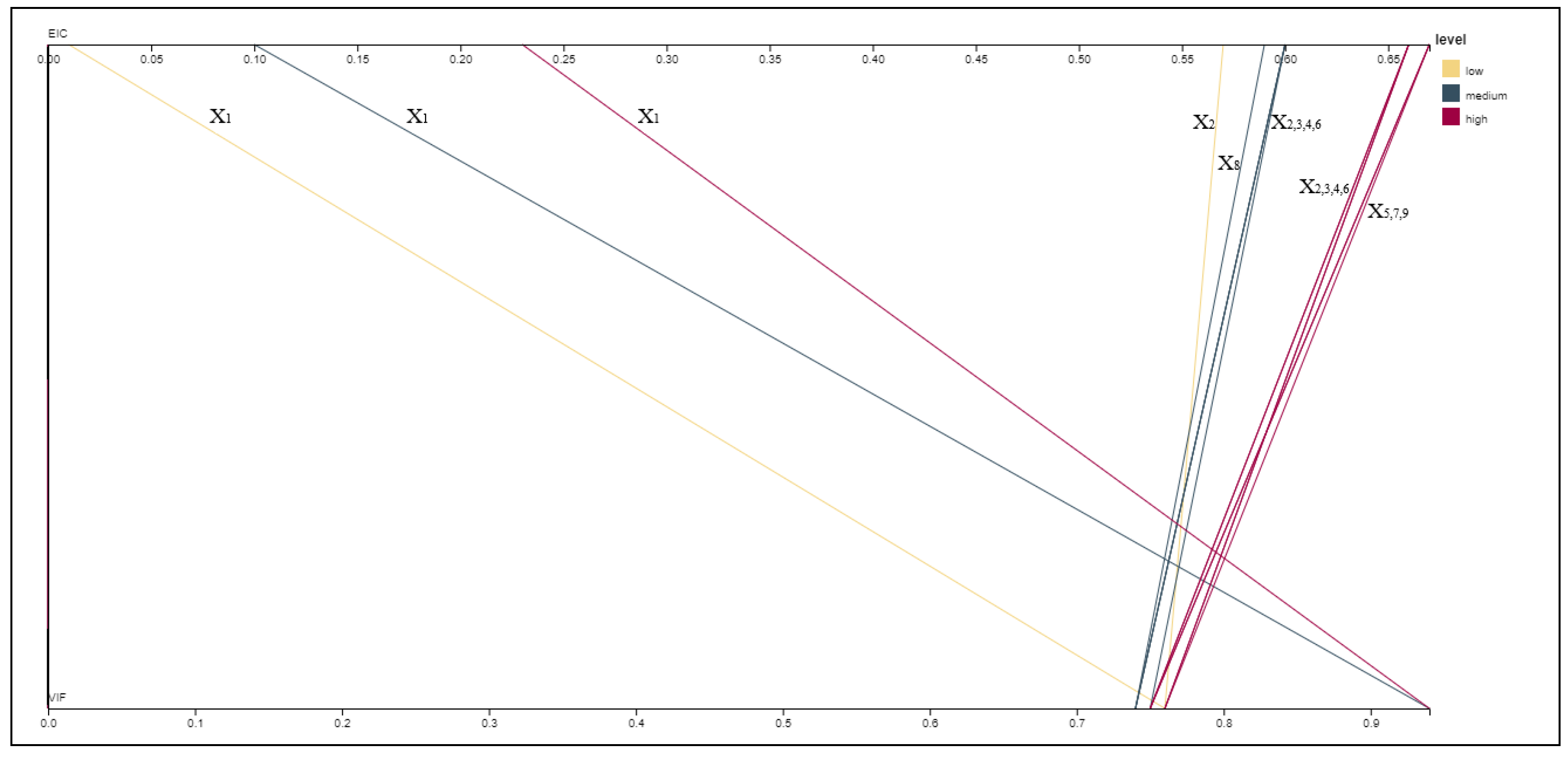
The Parallel Coordinates Graph (Figure 1), which was carried out in RAWGraphs (Mauri et al. (2017)), provides the percentage of times each $X_j$ variable appears as multicollinear based on EIC (upper line) and based on VIF (lower line) with yellow lines corresponding to low, green to the medium and red to the high correlation-based dataset. High values (close to 1, i.e., 100%) indicate extreme multicollinearity, while low values (close to 0, i.e., 0%) indicate weak (or absence of) multicollinearity. As an example, consider the yellow line (low correlation dataset) associated with the variable $X_1$ (which has been taken to be non-multicollinear). The EIC correctly identifies the non-multicollinearity of $X_1$ since the upper line is crossed at a value less than 0.05 (the actual value is 0.01). Meanwhile, VIF fails to identify the same. Indeed, although the yellow line should have been vertical (crossing the lower line at about the same value as the upper line) the crossing is observed far to the right, at a value between 70% and 80% (the actual value is 0.76) indicating that VIF characterizes, incorrectly, $X_1$ as multicollinear.

Based on the above observations according to Figure 1, we can conclude that only EIC succeeds in correctly identifying the level of multicollinearity of all variables involved with $X_1$ appearing on the left corner (of the upper line of Figure 1) and all others on the right corner. We also observe that as correlation increases (from yellow to red), VIF is deceived and fails to recognize the unaltered variable ($X_1$) but instead, it signifies it, falsely, as the most multicollinear variable, which may result in variable over-elimination and improper model selection.

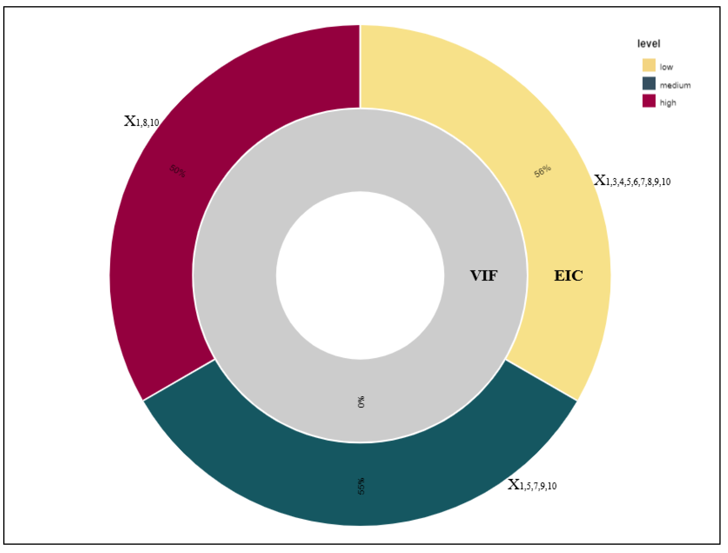
In the sunburst diagram (Mauri et al. (2017)) of Figure 2, one can see the percentage rate at which each measure (VIF in the inner circle and EIC in the outer circle) managed to properly do correct variable selection in each of the three categories. In Figure 2, VIF tends to do variable over-elimination and by expansion model misspecification. When the proper variables have been selected (all $X_j$ except $X_2$ for low, $X_1$, $X_5$, $X_7$, $X_9$, and $X_{10}$ for medium, $X_1$, $X_8$, and $X_{10}$ for high), then all the other (improper) variables have been selected too. Thus, one can state that the accuracy rate of proper variable selection based on VIF is 0%. On the contrary, the equivalent rate based on EIC surpasses 50% in all cases.

5. Conclusions

Conclusively, the suggested Elastic Information Criterion procedure results in a robust and easily interpretable methodology for handling multicollinearity along with the appropriate data-driven threshold. The criterion constitutes a novel shrinkage and selection method since it is based on both the coefficient of determination and beta coefficients penalization, emerging in virtue of a biased (towards the endpoints of the mixing parameter $\alpha$) Elastic Net, while the threshold has been established based on ${\lambda }_{j,en}$ tuning parameter of the same procedure. Thus, EIC is governed by the same or similar properties as those of Elastic Net. Additionally, it demonstrates a sufficiently sparse representative model with an adequate proper variable prediction rate, while firmly encouraging a grouping effect even when the significance of a variable is relatively limited.

The results of the real and simulated data analysis strongly suggest implementing EIC not only for econometric modeling and forecasting but also for classification purposes due to its high efficiency rate (Wooldridge (2014)). EIC does not commonly fail with highly correlated data as opposed to typically used measures for multicollinearity detection, while its high prediction accuracy is due to the restricted values of the parameter $\alpha$. Furthermore, EIC tends to perform better when the Elastic Net procedure is implemented at or near the ${\alpha }_{j,en}$ edges while it appears to have a robust variable selection accuracy rate over both real and simulated case studies. The pivotal characteristic of reduction or ejection of the insignificant coefficients that Elastic Net attains manages to enhance its efficiency rate. In comparison to other multicollinearity detection measures, it is evident that EIC prevails in terms of proper variable selection accuracy. An additional finding of this work is that the implementation of EIC can be vital in the field of econometrics, where interrelationships among variables frequently occur. Its capability to identify where (in which variable(s)) the troublesome multicollinearity lurks and penalize it accordingly minimizes a models’ bias without resulting in variable under or over-elimination.

EIC, as a criterion for implementing the Elastic Net mechanism, is particularly effective in tackling multicollinearity that lurks behind variables (Hastie et al. (2001); Zou and Hastie (2005)). Indeed, as displayed above in all levels and as compared with the most widely used measures, EIC (a) identifies the existence of patterns among variables, (b) is capable of recognizing and “selecting” the altered variables, leaving the unaltered ones intact, and (c) achieves extreme values in the presence of perfect multicollinearity and also in the total absence of it. Based on these characteristics and properties we can say that the effectiveness of EIC can place it high in the list of measures that can be used to address the multicollinearity issue and in that sense it can be considered as a useful and effective tool in the hands of the researcher to be used in conjunction with their judgment, experience, and knowledge together with any special features associated with the problem/dataset at hand.

In addition to the contributions of the proposed criterion to the multicollinearity literature, another advantage of EIC is that it operates as a variable/model selection criterion and consequently it can be exploited as a dimension reduction technique and thus, an alternative competitor to Principal Components Analysis and Linear Discriminant Analysis. It should be reminded that these classical dimension reduction techniques suffer from the fact that each generated component is a combination of different proportions of the original variables; thus it is often difficult to interpret the results (Zou et al. (2006)). On the other hand, the proposed EIC criterion manages to preserve the interpretability of the original variables because it relies simultaneously on shrinkage and sparse selection.

References

- Bayer, Sebastian. 2018. Combining Value-at-Risk Forecasts using Penalized Quantile Regressions. Econometrics and Statistics 8: 56–77. [Google Scholar] [CrossRef]
- Belsley, David A. 1991. A Guide to Using the Collinearity Diagnostics. Computer Science in Economics and Management 4: 33–50. [Google Scholar]
- Dumitrescu, Bogdan Andrei, Dedu Vasile, and Enciu Adrian. 2009. The Correlation Between Unemployment and Real GDP Growth. A Study Case on Romania. Annals of Faculty of Economics 2: 317–22. [Google Scholar]
- Farrar, Donald, and Robert Glauber. 1967. Multicollinearity in Regression Analysis: The Problem Revisited. The Review of Economics and Statistics 49: 92–107. [Google Scholar] [CrossRef]
- Fried, Joel, and Peter Howitt. 1983. The Effects of Inflation on Real Interest Rates. The American Economic Review 73: 968–80. [Google Scholar]
- Geary, Robert Charles, and Conrad Emanuel Victor Leser. 1968. Significance Tests in Multiple Regression. The American Statistician 22: 20–21. [Google Scholar]
- Greene, William H. 2002. Econometric Analysis, 5th ed. Hoboken: Prentice Hall. [Google Scholar]
- Gujarati, Damodar N., and Dawn C. Porter. 2008. Basic Econometrics, 5th ed. New York: Mc-Graw Hill. [Google Scholar]
- Hair, Joseph F., William C. Black, Barry J. Babin, and Rolph E. Anderson. 2010. Advanced Diagnostics for Multiple Regression: A Supplement to Multivariate Data Analysis, 7th ed. Upper Saddle River: Pearson Education. [Google Scholar]
- Halkos, George, and Kyriaki Tsilika. 2018. Programming Correlation Criteria with free CAS Software. Computational Economics 52: 299–311. [Google Scholar] [CrossRef]
- Hastie, Trevor, Robert Tibshirani, and Jerome H. Friedman. 2001. The Elements of Statistical Learning: Data Mining, Inference, and Prediction. New York: Springer. [Google Scholar]
- Imdadullah, Muhammad, Muhammad Aslam, and Saima Altaf. 2016. mctest: An R Package for Detection of Collinearity among Regressors. The R Journal 8: 495–505. [Google Scholar] [CrossRef]
- Kendall, Maurice G. 1957. A Course in Multivariate Analysis. New York: Hafner Pub. [Google Scholar]
- Klein, Lawrence R. 1962. An Introduction to Econometrics. Englewood Cliffs: Prentice Hall. [Google Scholar]
- Kovács, Péter, Tibor Petres, and László Tóth. 2005. A New Measure of Multicollinearity in Linear Regression Models. International Statistical Review/Revue Internationale de Statistique 73: 405–12. [Google Scholar] [CrossRef]
- Lindner, Thomas, Jonas Puck, and Alain Verbeke. 2020. Misconceptions about Multicollinearity in International Business Research: Identification, Consequences, and Remedies. Journal of International Business Studies 51: 283–98. [Google Scholar] [CrossRef] [Green Version]
- Liu, Wenya, and Qi Li. 2017. An Efficient Elastic Net with Regression Coefficients Method for Variable Selection of Spectrum Data. PLOS ONE 12: e0171122. [Google Scholar] [CrossRef] [PubMed]
- Mauri, Michele, Tommaso Elli, Giorgio Caviglia, Giorgio Uboldi, and Matteo Azzi. 2017. RAWGraphs: A Visualisation Platform to Create Open Outputs. In Proceedings of the 12th Biannual Conference on Italian SIGCHI Chapter. Association for Computing Machinery. New York: Association for Computing Machinery. [Google Scholar]
- Ntotsis, Kimon, and Alex Karagrigoriou. 2021. The Impact of Multicollinearity on Big Data Multivariate Analysis Modeling. In Applied Modeling Techniques and Data Analysis. London: iSTE Ltd., pp. 187–202. [Google Scholar]
- Ntotsis, Kimon, Emmanouil N. Kalligeris, and Alex Karagrigoriou. 2020. A Comparative Study of Multivariate Analysis Techniques for Highly Correlated Variable Identification and Management. International Journal of Mathematical, Engineering and Management Sciences 5: 45–55. [Google Scholar] [CrossRef]
- Oner, Ceyda. 2020. Unemployment: The Curse of Joblessness. International Monetary Fund. Available online: www.imf.org/external/pubs/ft/fandd/basics/unemploy.htm (accessed on 29 November 2021).
- Organisation for Economic Co-operation and Development. 2021. OECD Main Economic Indicators (MEI). Available online: https://www.oecd.org/sdd/oecdmaineconomicindicatorsmei.htm (accessed on 10 August 2021).
- Perez-Melo, Sergio, and B. M. Golam Kibria. 2020. On Some Test Statistics for Testing the Regression Coefficients in Presence of Multicollinearity: A Simulation Study. Stats 3: 40–55. [Google Scholar] [CrossRef] [Green Version]
- Silvey, Samuel D. 1969. Multicollinearity and Imprecise Estimation. Journal of the Royal Statistical Society. Series B 31: 539–52. [Google Scholar] [CrossRef]
- Theil, Henri. 1971. Principles of Econometrics. New York: John Wiley & Sons. [Google Scholar]
- Tibshirani, Robert. 1996. Regression Shrinkage and Selection via the Lasso. Journal of the Royal Statistical Society. Series B 58: 267–88. [Google Scholar] [CrossRef]
- Tikhonov, Andrei Nikolajevits. 1943. On the Stability of Inverse Problems. Doklady Akademii Nauk SSSR 39: 195–98. [Google Scholar]
- Tikhonov, Andrei Nikolajevits. 1963. Solution of Incorrectly Formulated Problems and the Regularization Method. Soviet Mathematics 4: 1035–38. [Google Scholar]
- Trading Economics. 2021. Main Indicators. Available online: https://tradingeconomics.com/indicators (accessed on 7 November 2021).
- Ueki, Masao, and Yoshinori Kawasaki. 2013. Multiple Choice from Competing Regression Models under Multicollinearity based on Standardized Update. Computational Statistics and Data Analysis 63: 31–41. [Google Scholar] [CrossRef]
- Ullah, Muhammad, Muhammad Aslam, Saima Altaf, and Munir Ahmed. 2019. Some New Diagnostics of Multicollinearity in Linear Regression Model. Sains Malaysiana 48: 2051–60. [Google Scholar] [CrossRef]
- Weisburd, David, and Chester Britt. 2013. Statistics in Criminal Justice. Berlin/Heidelberg: Springer Science and Business Media. [Google Scholar]
- Wooldridge, Jeffrey M. 2014. Introduction to econometrics: Europe, Middle East and Africa Edition. Boston: Cengage Learning. [Google Scholar]
- World Bank Open Data. 2021. Available online: data.worldbank.org (accessed on 15 August 2021).
- Yue, Lili, Gaorong Li, Heng Lian, and Xiang Wan. 2019. Regression Adjustment for Treatment Effect with Multicollinearity in High Dimensions. Computational Statistics and Data Analysis 134: 17–35. [Google Scholar] [CrossRef]
- Zou, Hui, and Trevor Hastie. 2005. Regularization and Variable Selection via the Elastic Net. Journal of the Royal Statistical Society, Series B 67: 301–20. [Google Scholar] [CrossRef] [Green Version]
- Zou, Hui, Trevor Hastie, and Robert Tibshirani. 2006. Sparse Principal Component Analysis. Journal of Computational and Graphical Statistics 15: 265–86. [Google Scholar] [CrossRef] [Green Version]
Figure 1.
The Parallel Coordinates Graph—the proportion of times each variable appears as multicollinear based on VIF (lower line) and EIC (upper line) in three (low/yellow—medium/green—high/red) correlation categories. Only variables with non-zero proportions are displayed.
Figure 2.
Proper model selection based on EIC and VIF for all three correlation-based categories.