1. Introduction
Floods constitute a real and continuing threat to lives, infrastructure and environment throughout much of the world. In recent years the intensity and frequency of flood has been increasing arguably as a result of climate change. The UK is no exception to this. The recent major floods including the catastrophic 2007 summer floods have triggered widespread concern of flood risk and the need for a sustainable approach to flood risk management [
1].
Identification and assessment of flood risk requires modelling of floodplain inundation that allows land owners and river basin managers to make informed decisions on how to manage the risk. Spatially explicit hydrodynamic flood models can play an important role in producing such inundation maps. A key element of these models that make them suitable for flood risk assessment is the ability to provide time-series inundation information about the onset, duration and passing of a flood event [
2]. Such information is critical for strategic planning of flood defence measures and effective flood risk management.
Advanced deterministic methods of floodplain inundation generally consist of construction of a physically-based fully 2D hydrodynamic model, calibration of the model using historical flood data, use of the best-fit model to simulate synthetic design flood events and interpretation of the model results to generate flood-hazard maps in a Geographical Information System (GIS) environment [
3,
4,
5]. Performance of deterministic models depends on many factors such as cross-section configuration, mesh resolution, representation of river bathymetry and modelling approach [
6].
The lack of empirical and real world data to parameterize and validate the output of the models is one of the limitations of the distributed hydrodynamic modelling approach [
7]. However, the recent increased availability of distributed remote sensing data has helped to address this issue and also allowed considerable progress in the field-scale application and testing of a wide variety of 2D flood inundation models [
8,
9]. Light Detection and Ranging (LiDAR) data, for example, provide a wealth of topographic information that is widely used in floodplain mapping [
4,
7,
10]. Such data can be used to create Digital Terrain Models (DTMs) required for producing flood inundation maps using 2D hydrodynamic models. LiDAR can also be used to precisely locate water courses and define a suitable height contour that is useful for defining the extent of the model domain [
10].
Despite the availability of detailed topographic data, there is a lack of long-term observational data especially on river flow discharge in many parts of the rural catchments in Scotland. This may result in the extreme flow events being inaccurately estimated. However, shot-term data, if available, can also be utilized to provide estimates of flow discharge to model flood inundation from larger and less frequent events using data sets from “hydrologically” similar gauged catchments. Application of such techniques in 2D hydrodynamic modelling for ungauged rural river catchments is limited. This paper describes a modelling approach to floodplain mapping where only short-term data set is available on rainfall and flow discharge and there is limited information available on observed flood events. In this study, a fully 2D hydrodynamic model has been applied to develop catchment-scale flood inundation maps from a set of storm events of varying return periods. Furthermore, the model is tested to simulate a past storm event in terms of flood inundation at a local scale.
2. Study Area
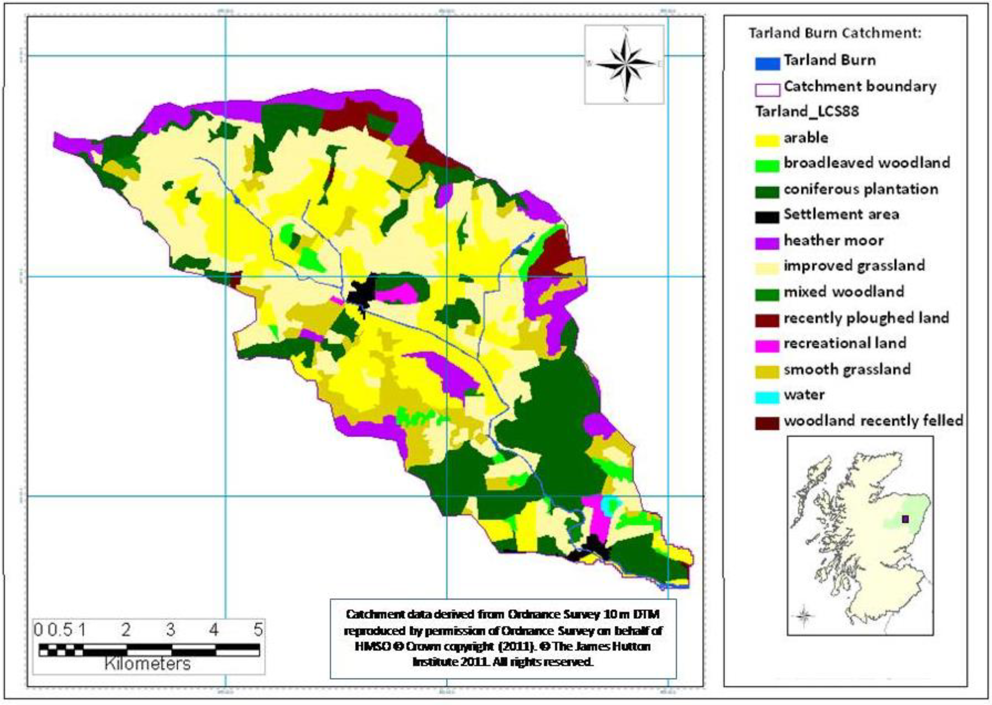
The Tarland Burn (74 km
2), a sub-catchment of the River Dee catchment (2,105 km
2) is located in Aberdeenshire, north-east Scotland (
Figure 1). The Tarland Burn catchment land use is typical for many agricultural regions of Northeast Scotland, in which the major land uses are arable (25%), plantation forestry (19%), improved and unimproved grassland (36% and 10% respectively), heather moorland (8%) and mixed/broadleaved woodland (2%) [
11]. The two main settlements in the catchment are Tarland and Aboyne.
Figure 1.
The study area of Tarland Burn catchment (derived from Ordnance Survey 10 m Digital Terrain Model (DTM), reproduced by permission of Ordnance Survey.
Figure 1.
The study area of Tarland Burn catchment (derived from Ordnance Survey 10 m Digital Terrain Model (DTM), reproduced by permission of Ordnance Survey.
The Tarland Burn and its tributaries have been extensively deepened and straightened to drain the surrounding floodplain and wetlands for the benefit of agriculture [
12]. The isolation of the natural floodplain and removal of wetland “storage” zones that used to dominate the lower valley bottom may have led to an increase in flood risk on several areas including Tarland and Aboyne. The area has witnessed several flood events in the recent past. Aberdeenshire Council’s Biennial Reports on flooding indicated that flooding incidents occurred in April 2000, October 2002, December 2005, March 2006 and most recently in July 2009 and May 2010. The flooding of April 2000 damaged many private dwellings and public roads in Tarland and Aboyne. Also some commercial premises were flooded in Aboyne.
This study was undertaken on a 7 km reach of the Tarland Burn (
Figure 1). The Coull Bridge gauging station operated by the James Hutton Institute is located within the middle reaches of the catchment. The catchment area at the gauge is approximately 51 km
2. Installed in 1999, the gauging station records water level every 30 s and the values are averaged and stored every 15 min and every hour using a sonic ranging sensor (SR50).
3. Methodology
3.1. Flood Frequency Analysis
A statistical tool called “WINFAP-FEH” (Version 3) has been used to undertake flood frequency analysis based upon the Flood Estimation Handbook (FEH) method which is recognized as the best practice method for estimating peak flood discharge especially from ungauged catchment. The method essentially involves estimation of the index flood which is the median annual maximum flood (QMED), defining a polling group for the catchment of interest involving hydrologically “similar” catchments, development of a flood growth curve using the pooling group data and derivation of flood frequency curve as the product of QMED and the flood growth curve for a give return period. The QMED represents a typical magnitude of flood which has a return period of two years and is estimated using the following equation based on the use of a set of catchment descriptors essentially for rural catchments [
13]:
where AREA is the catchment area (km
2), SAAR is the standard average annual rainfall(mm) based on measurements from 1961–1990, FARL is an index of flood attenuation due to reservoirs and lakes and BFIHOST is the base flow index derived from HOST soil data. All of these parameters are readily available and are obtained from the Flood Estimation Handbook (FEH) CD ROM.
As estimating QMED using two years’ flow data generally provides a better estimate than the catchment descriptors method [
14], QMED has also been estimated using the flow gauge data and compared with the QMED estimated using Equation (1).
where,
Qt is peak flow in m
3/s, QMED is median annual maximum flood, m
3/s and
ZT is flood growth curve. A flood growth curve is constructed by fitting a probability distribution to the observed annual maxima (AM) data series. The Generalised Logistic (GL) distribution has been recommended for fitting values of extremes for the UK flood data series [
15] and therefore has been used in this study.
Flood frequency analysis is generally undertaken in two ways. The method of single site analysis is based upon the observed peak flow data series at the target catchment alone and thus not applicable to ungauged catchments. The pooled analysis, on the other hand, is applied to an ungauged catchment based on a set of catchment characteristics to identify a number of gauged catchments (often called donor catchments) which can be considered hydrologically similar to the target catchment. The observed flow data for the donor catchments are then used to estimate peak flows at the ungauged target catchment. For a given distribution, a growth curve for the subject site is estimated as a weighted average of the single-site growth curves for the catchments in the pooling groups and the weightings are a function of the record length and similarity to the subject site [
13]. In this study both single site and pooling group methods have been considered. In the pooled analysis, the limited flow gauge data of the study area (subject site) have been included in the initial pooling group which gives a greater weighting factor reflecting the importance of the on-site data. Details about the procedure are given in [
15].
3.2. Estimation of Design Flow Events
As the site has a limited rainfall and flow records, design events are estimated using the FEH statistical rainfall runoff method based on a set of catchment descriptors parameters [
15]. For this, a software package called ISIS (Version 3.4) was used where the FEH rainfall runoff method is available as a model boundary unit (FEHBDY) (
http://www.halcrow.com-/isis/). It is acknowledged that the design flow hydrographs developed using this method can be inaccurate if the parameter estimation is based solely on catchment descriptors. Hence, in order to address the uncertainty issues to some degrees, some representative observed rainfall-runoff events were selected and used for the calibration of the model. Adjusted parameters are the time base and the peak flow of the unit hydrograph to match the observed and modelled flow hydrographs for each selected storm event. Estimation of design flow hydrographs is based on the average of the adjusted unit hydrograph parameters for a given return period. The base flow component of the model has been estimated based on the catchment descriptors as no reliable records are available. Following equations are used for estimating unit hydrograph parameters based on catchment descriptors:
where T
p (0) is the time to peak of the instantaneous unit hydrograph (hours), Tp (t) is the time to peak of t-hour unit hydrograph (hours), Q
p is peak flow of the t-hour unit hydrograph (m
3/s), CAREA is the catchment area (km
2), t is data interval (hours) and TB is the time base of the unit hydrograph (hours). Similarly, DPSBAR is mean drainage path slope (m/km), PROPWET is proportion of time when the soil moisture deficit (SMD) was equal to or below 6 mm during 1961–1990, DPLBAR is mean drainage path length (km) and URBEXT is extent of urban and suburban land cover and these parameters are usually obtained from the FEH CD-ROM. The design storm duration is estimated using the following equation:
Development of Model
The 2D model (TUFLOW, BMT WBM, Build 2011) was applied to the study reach. TUFLOW is a computational hydrodynamic model used to simulate the flow of water along channels and across surfaces. Full details about the model can be found at
http://www.tuflow.com. Essentially the model solves the shallow water equations to model 2D flows e.g. [
16].
The approach adopted in this study includes modelling of the channel as a 1D network nested within the 2D domain representing the floodplain. For this the catchment was divided into a network of small grids and cells. A cell is the smallest unit of model computation. A 5m cell was considered appropriate considering the size of the channel and computational time required to run the model. A ground Digital Elevation Model (DEM) was then developed using the LiDAR data of 1m resolution by transferring elevations to the centre of each cell. This was done by using Vertical Mapper tools available in Map Info (PitneyBowes, Professional Version 10.5.2). The extents of the 2D domain were defined based on the general land topography which mostly included the low-lying floodplain areas that are likely to be flooded. The purpose of defining the 2D domain was to save computational time by excluding permanently dry areas such as hillslopes that would not be flooded. The channel cross sections were taken from ground surveys undertaken between March 2007 and January 2009 and used to define the hydraulic geometry of the main channel. Where the survey data were not available, cross sections were generated from the LiDAR DEM.
The channel roughness or bed resistance values (e.g., Manning’s n) were assigned based on the current land use as suggested in the literatures [
17]. The roughness coefficient for the main channel was estimated by undertaking modelling analysis of a past flood event where some records on the inundation area were available. The roughness coefficients considered for the floodplain were: arable land-0.06, road-0.025, ponds and water bodies-0.030, buildings including rear gardens-2.00, vegetative creek-0.08 and riparian vegetation-0.200. Sensitivity tests were carried out to see how these assumed values will affect the model output. An important aspect of the modelling approach is to define the topographic boundary condition based on the existing embankment levels. This is done by using 1D/2D linkages where there is flow interchange between the 1D and 2D components of the model. These links are essentially located along the top of the banks on each side of the channel. This component is of extreme importance as the lines define where flow will interact between the 1D channel and the 2D floodplain. Attempts were made to define the bank top lines as precisely as possible with the help of the LiDAR DEM and field checks were undertaken where they were not clearly visible on the DEM. The model upstream boundary was represented as a flow-time boundary and the downstream as a flow-head boundary, both estimated using the FEH techniques. A range of hydrological events with different return periods were considered and flow hydrographs were derived.
The time series output (such as flow depth and velocity) from the model were processed using the Surface-Water Modelling System (SMS Aquaveo, Version 10.1) software to develop flood inundation maps. The model output can also be imported and viewed in any GIS platform.
4. Results
4.1. Flood Frequency Estimation
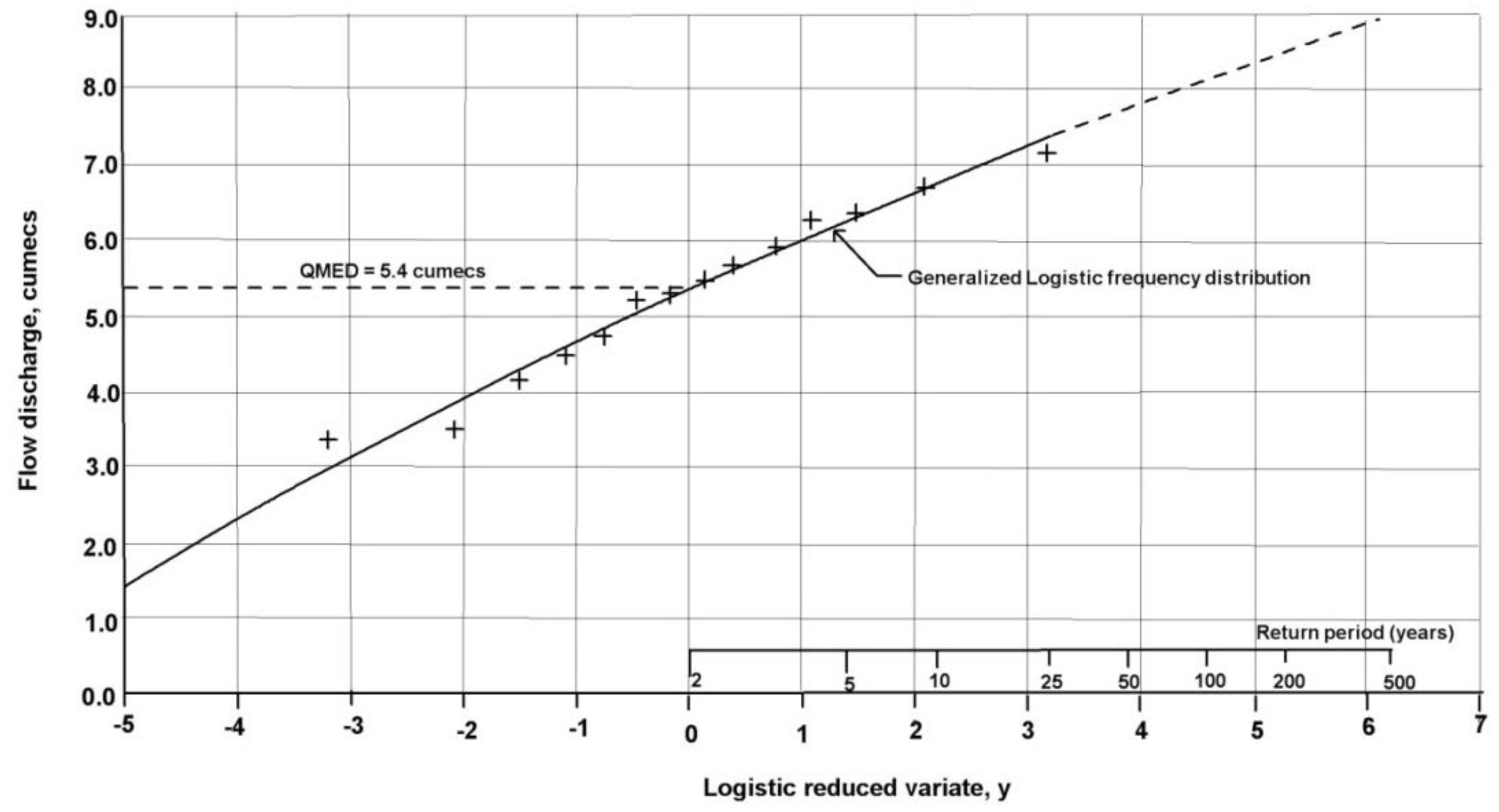
The flood frequency curve derived by using the single site analysis based on the Generalised Logistic (GL) frequency distribution (
Figure 2).
Figure 2 shows that the highest recorded flow event of 7.2 m
3/s corresponds to a return period of 1 in 25 years. The extended fitting curve indicates a peak flow discharge of 8.2 m
3/s and 8.5 m
3/s that correspond to approximately 1 in 100 years and 1 in 200 years respectively. There was a good agreement between the observed and FEH catchment descriptors derived estimates of QMED (5.40 m
3/s and 5.27 m
3/s respectively). The data transfer ratio of 1.024 (
i.e., ratio of QMED observed and QMED FEH derived) was used to estimate the flood frequency of the subject site.
Figure 2.
Flood frequency curve at Coull, Tarland derived using single site method.
Figure 2.
Flood frequency curve at Coull, Tarland derived using single site method.
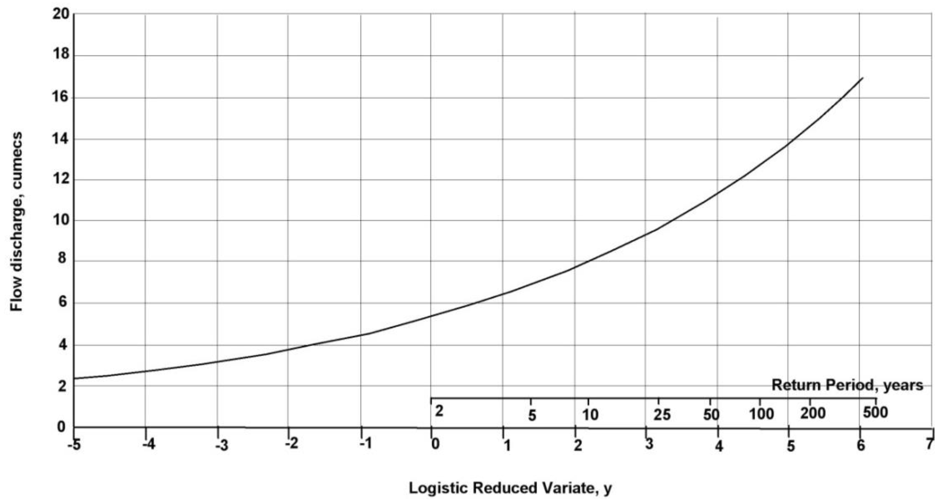
In the pooling group method, a total of 9 gauging stations (donor catchments) were selected which provided a total of 306 years of flow data. Some stations with data not suitable for either pooling or estimation of QMED were discarded from the pooling group. The flood frequency analysis is based on the GL frequency distribution (
Figure 3). The estimated flood discharges for a range of return period are summarized in
Table 1.
Table 1 indicates that there is no significant difference between the flow estimates provided by each of the methods for smaller and more frequent events, mostly up to 1 in 5 years. Comparing these against the higher and rarer events, it can be seen that the flow estimates derived from the pooling method appear to be over-estimated by 55% and 72% for the 1 in 100 year and 1 in 200 year events respectively. As the pooling method is based on the larger data set of observed events and is particularly important for the rare events, the flow estimates derived from this method are taken forward for the estimation of design flows required to develop inflow hydrographs for the model.
4.2. Estimation of Design Flows
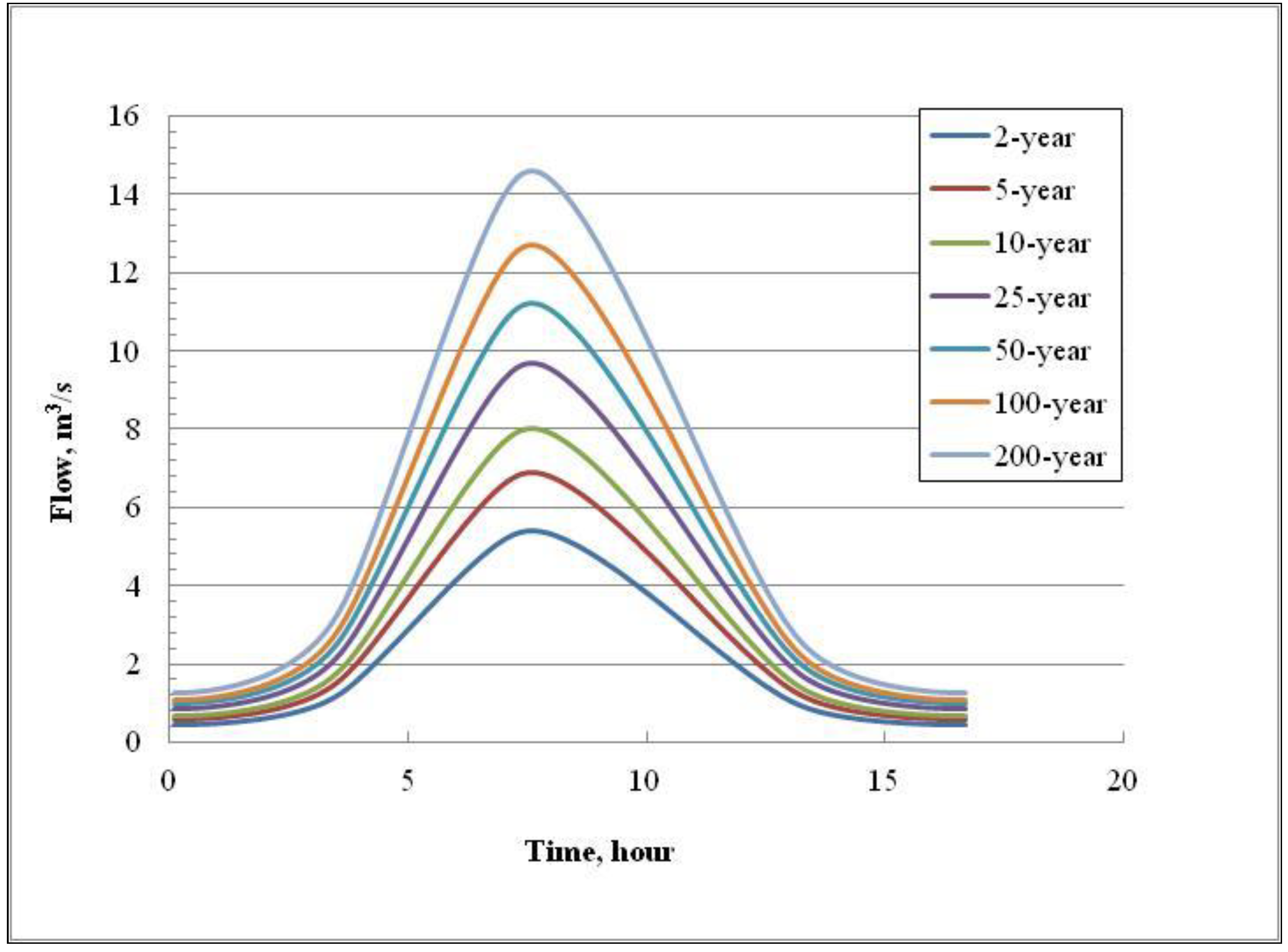
The design flow events of a range of return periods estimated based on a set of catchment descriptor parameters are shown in
Figure 4. The estimated unit hydrograph time to peak is approximately 8 h and the estimated design storm duration is 16 h. The design flow hydrographs at Coull gauging station were scaled up based on the drainage area to estimate design flow hydrographs upstream of Tarland village. Here, it is assumed that the land use, topography and other characteristics of the sub-catchment between the Tarland village and Coull are similar to that of entire catchment upstream of Tarland.
Figure 3.
Flood frequency curve at Coull, Tarland derived using the pooled method.
Figure 3.
Flood frequency curve at Coull, Tarland derived using the pooled method.
Table 1.
Flood discharge estimates for different return periods.
Table 1.
Flood discharge estimates for different return periods.
| Methods | 1 in 2 years | 1 in 5 years | 1 in 10 years | 1 in 25 years | 1 in 50 years | 1 in 100 years | 1 in 200 years |
|---|
| Single site (m3/s) | 5.4 | 6.3 | 6.8 | 7.4 | 7.8 | 8.2 | 8.5 |
| Pooling (m3/s) | 5.4 | 6.9 | 8.0 | 9.7 | 11.2 | 12.7 | 14.6 |
Figure 4.
Design flow hydrographs.
Figure 4.
Design flow hydrographs.
4.3. Development of Flood Inundation Map
4.3.1. Modelling of a Past Storm Event
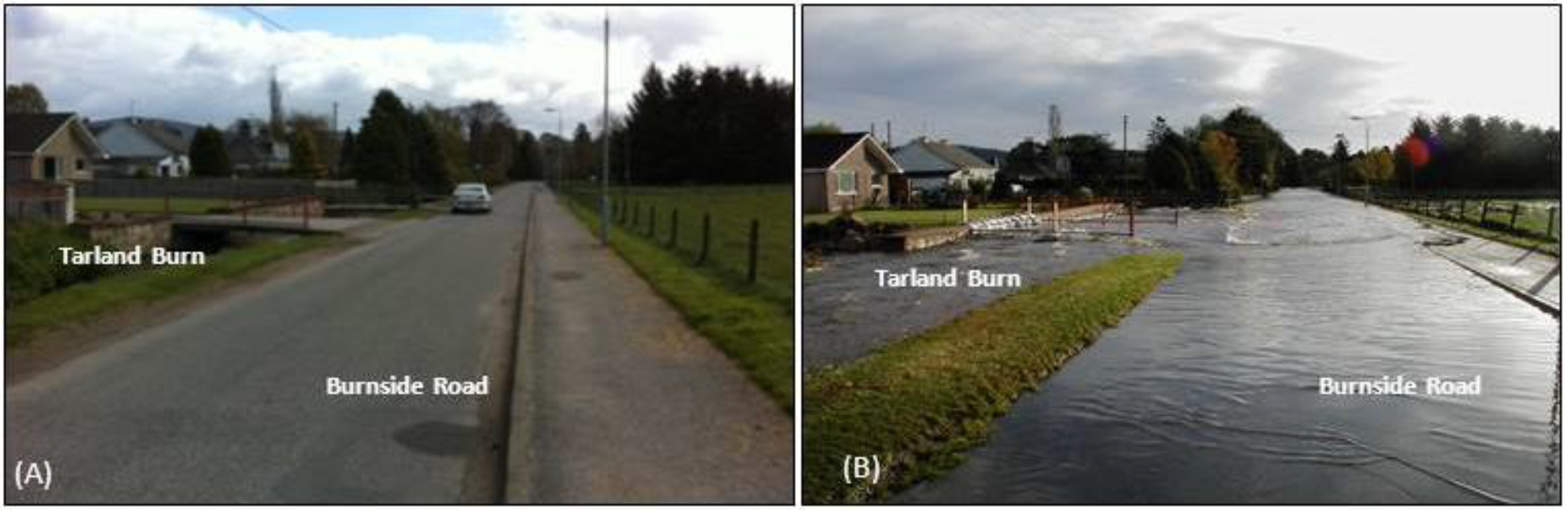
Around the southern outskirts of Tarland village the channel overtopped its banks as a result of a storm event in October 2002 affecting many residential properties along the Burnside Road (
Figure 5). This event was analysed and modelled using the flow data from the Coull Bridge gauging station. The flood discharge data of Coull was downscaled based on the ratio of catchment area to estimate flood discharge at the upstream of Tarland, which was then utilized as direct inflow at the model upstream boundary. The flow hydrograph indicates a maximum instantaneous discharge of 5 m
3/s, which is approximately equivalent to the index flood;
i.e., 1 in 2 year probability of occurrence (
Figure 2).
Figure 5.
The Burnside Road of Tarland village (A) During the normal condition (B) During the flood of October 2002 looking downstream.
Figure 5.
The Burnside Road of Tarland village (A) During the normal condition (B) During the flood of October 2002 looking downstream.
The channel roughness coefficient was found to be the key model parameter. This parameter was adjusted in a bid to match the observed and modelled flood extents around the Burnside Road. It is important to note that the comparison between the observed and modelled flood extents was undertaken by visual examination and judgment as the observed flood extent was very small and localized within a very short stretch of the channel. Hence, no statistical assessment has been undertaken to compare the flood extents. A lumped roughness coefficient of 0.040 resulted in a best fit of the model output with the observed flood event (
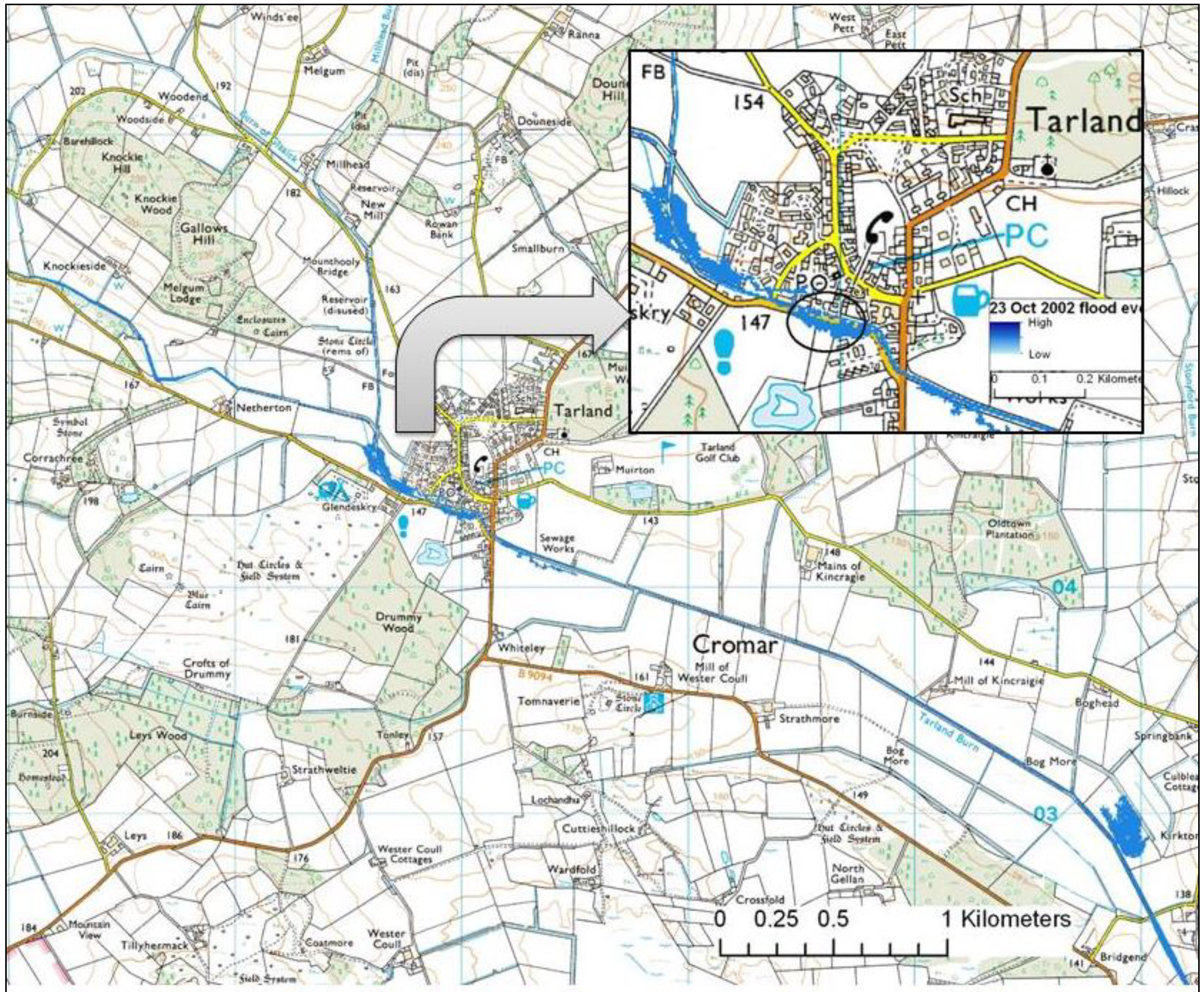
Figure 5) and was considered appropriate to represent the overall channel condition. The flood inundation map for this event is shown in
Figure 6. The inundation map indicates that the channel overtopped its right bank that led to the Burnside Road being completely inundated as evident from the photograph taken at the time of the event (
Figure 5B). This suggests that the model was able to simulate this particular flood event reasonably well.
4.3.2. Catchment-Scale Flood Inundation Modeling
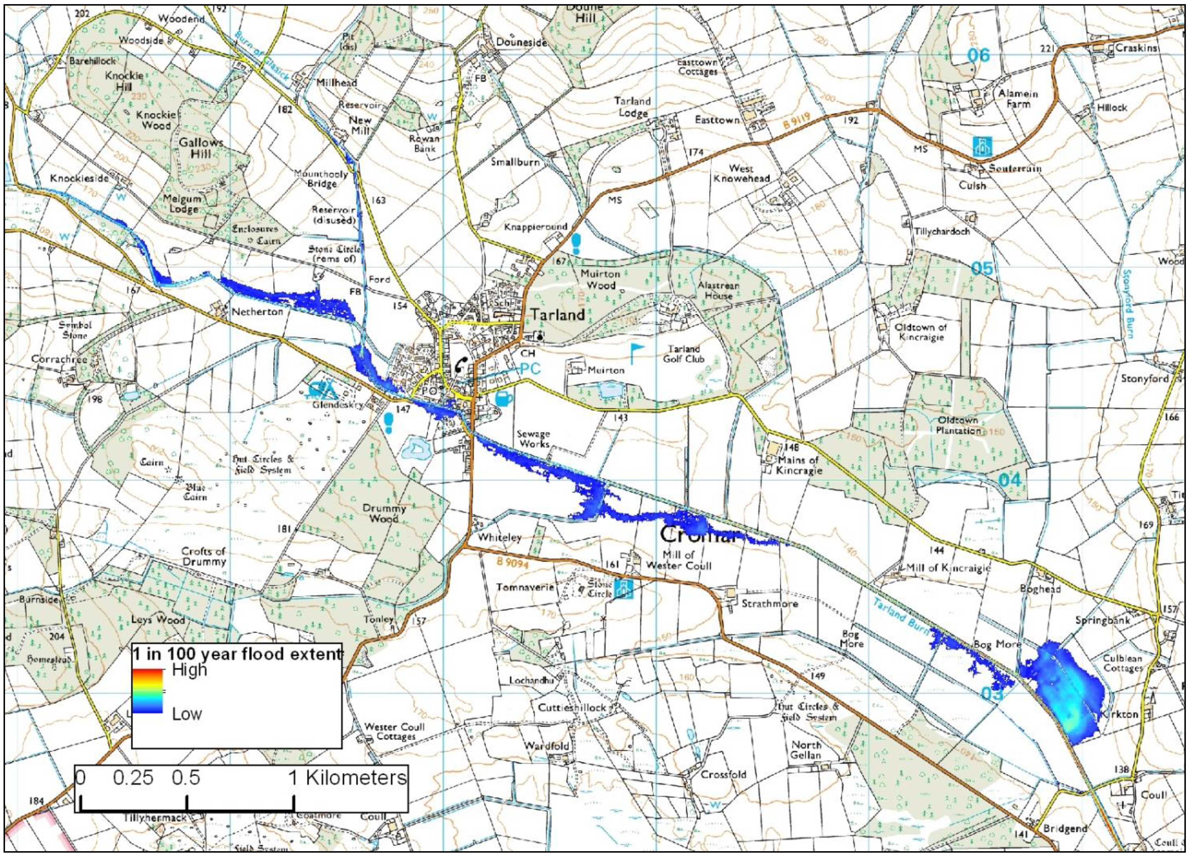
At the catchment scale, flood inundation analysis was undertaken using a set of estimated design events of different return period. An example of the flood inundation map developed for an extreme event with a 1 in 100 year probability of occurrence is shown in
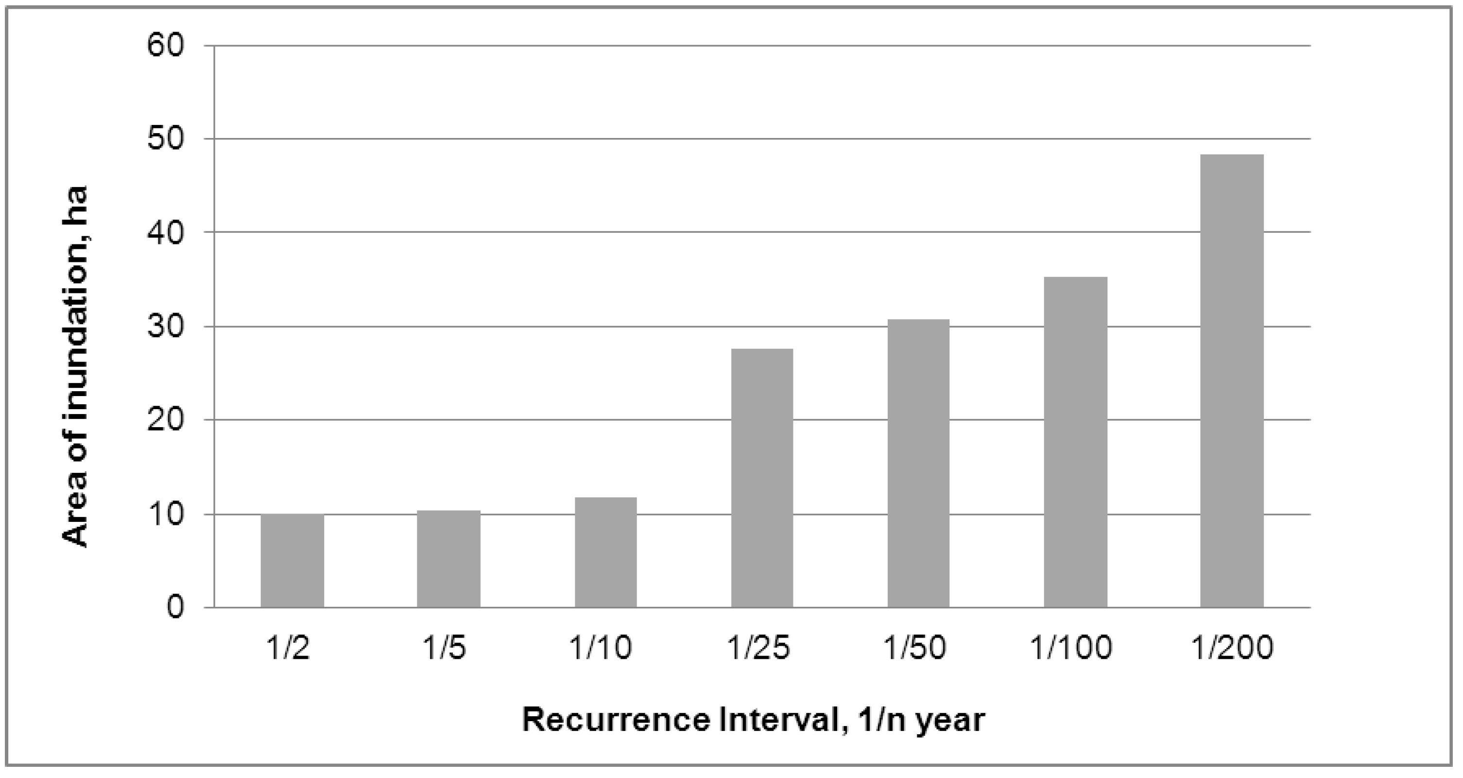
Figure 7 which indicates that many residential houses of Tarland village and agricultural fields located adjacent to the main channel will be flooded. The map also indicates the spatial distribution of the flood depth which varies from a few centimetres to as high as 0.80 m. Inundated area against a set of storm events is shown in
Figure 8. It indicates that relatively small magnitude and more frequent storm events (up to 1 in 10 years) result in approximately 10 ha of land being flooded. Approximately 35 ha of land will be flooded by an extreme storm of 1 in 100 year. The inundated land will increase to approximately 50 ha for an extreme event of 1 in 200 year.
Figure 6.
Flood inundation map for the October 2002 flood event. At the centre of the circle is the flood inundation around the Burnside Road.
Figure 6.
Flood inundation map for the October 2002 flood event. At the centre of the circle is the flood inundation around the Burnside Road.
Figure 7.
1 in 100 year extreme flood inundation of Tarland.
Figure 7.
1 in 100 year extreme flood inundation of Tarland.
Figure 8.
Flood inundation area under different recurrence interval storm events.
Figure 8.
Flood inundation area under different recurrence interval storm events.
5. Discussion
Given the limited range of record lengths at the study site, extrapolation of properties of flow regimes across the homogeneous regions through the regionalization technique can be a source of uncertainty. The UK Flood Estimation Handbook (FEH) recommends that estimating flood event magnitudes from catchment properties and regional climatology should be based on the transfer of analogous data from sites (
i.e., donor sites) that are hydrologically similar in terms of rainfall, catchment area and soil types. However, in practice it is difficult to establish an appropriate set of donor sites. Furthermore, there might be uncertainty as a result of classification of different sites into similar grouping. There may be fundamental difference between sites that would result in the transfer of inappropriate information and the production of inaccurate flood estimates [
18].
The FEH involves the use of an index flood procedure to derive the flood frequency curve at ungauged sites. This procedure is based on the assumption that donor sites have the same flood frequency distribution but differ in terms of the index flood. The index flood is thus taken as a scaling factor for the growth curve which is estimated from catchment characteristics. Flood magnitudes estimated from catchment descriptors are less accurate than flood peak data [
19]. It is therefore important to check and verify the estimates both from the catchment descriptors and peak flow data if available. In the present study, there was a good match between the index flood estimates derived from the two methods. However, as the estimates of the index flood is based on the flood peak data of very limited period, care must be taken when up-scaling index flood especially for higher return period events which are typically longer than the record period.
The model simulates flow series representative of the time horizon considered. The flood regime of a catchment is often described through a flood frequency curve. It considers only on a selection of the highest flows which assumes that the flow regime is stationary and the data that have been sampled to construct the flood frequency curves are drawn from a distribution which is not changing. In the absence of reliable climate models, the assumption of stationarity around the time horizon of interest is useful for assessing impacts of future climate on flood risks [
20]. Standard probability techniques remain valid under this assumption and thus resulting flood frequency curves are considered representative of the flood regime of the considered time horizon.
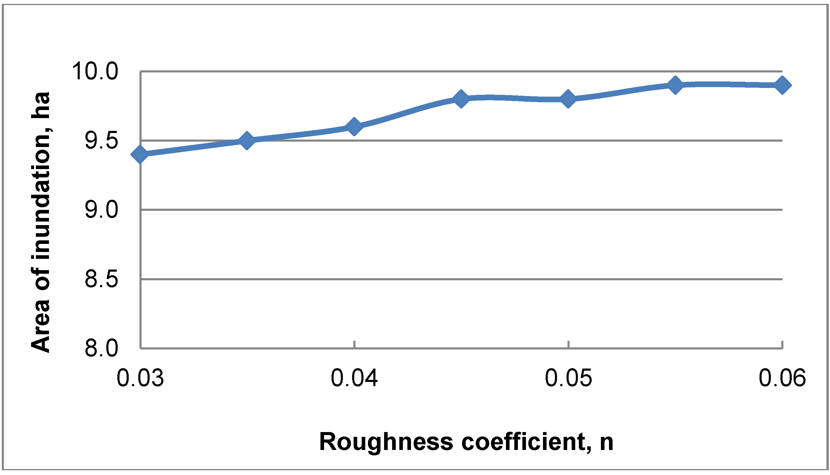
A range of sensitivity tests were performed in order to ascertain how uncertainties in model parameters impact on the robustness of the model output. The key parameters considered in this study were 1D and 2D roughness coefficients. In the case of 1D roughness coefficient, it was determined that a value of 0.040 will adequately represent the roughness condition of the channel mostly covered by small shrubs and vegetation. The inundated areas for a range of roughness coefficients are shown in
Figure 9. When the roughness decreases from 0.040 to 0.030, the inundated area will decrease from 9.6 ha to 9.4 ha. Similarly, when the roughness increases from 0.04 to 0.045, the inundated area increases from 9.6 ha to 9.8 ha and for further increase to 0.06 will lead to an inundated area which is approximately 10 ha. This shows that the 1D roughness parameter is not very sensitive in terms of the inundated area. Similarly, sensitivity test for the roughness of the agricultural land which was the dominant land use within the floodplain, indicated that the model sensitivity to the change in floodplain roughness was not very significant.
Figure 9.
Sensitivity analysis of 1D channel roughness coefficient.
Figure 9.
Sensitivity analysis of 1D channel roughness coefficient.
The capability of 2D hydraulic models depends on how well the channel flow conveyance and the channel form and bed topography are represented within the model domain. High resolution digital elevation models (DEMs) acquired by airborne laser altimetry (LiDAR) enable the raster-based 2D models to incorporate channel form, bed topography and floodplain geometry more accurately [
4], however, the use of LiDAR has also some important limitations. The bed topography of relatively narrow and deep channels cannot be well represented by LiDAR. Furthermore, vegetation can hinder the accuracy of LiDAR. In the present study, LiDAR generated channel bed topography was compared with the one obtained from field survey. The comparison shows a marked difference in the channel bed topography obtained from these two sources. The difference is significant typically within the channel bed and side slopes with a maximum difference of 15 cm. In contrast, LiDAR represent the floodplain topography very well as evident from the close match between the LiDAR and field survey levels around the bank tops on each side.
Model parameterization and validation is a typical problem of most distributed hydraulic models given due to the paucity of detailed data on flow discharge, channel form and bed topography [
8]. In this study, the key model parameter
i.e., bed roughness coefficient is optimized based on a single flood event for which evidence of flood inundation was available. Uncertainty in the model parameters will increase as a result of a combination of various hydrological processes at different spatial-temporal scales. Furthermore, accurate measurement of extreme flow events may not be possible when water levels exceed gauging limits and start to flow into the floodplain. These all sources of uncertainty should be considered for making a more reliable and accurate estimates of extreme flows.
6. Conclusions
Modelling of flood inundation from extreme rainfall events is a challenge, particularly in many parts of rural catchments of Scotland where there is a lack of long-term observational data, especially on river flow discharge. The study presents the findings from the application of a 2D hydraulic modelling approach to floodplain inundation in a Scottish rural catchment where only limited observation data on flow discharge is available. The FEH flood frequency estimation technique was applied to provide estimates of flow discharge from the extreme events of different probability of occurrences. It was found that there was a good match in the estimates of flow discharge using the single site and the FEH’s pooling group method for the events up to 1 in 5 year return period. For higher and rare events, flow estimates were made using the data set from hydrologically similar gauged catchments applying the techniques of the pooling group method, as it is based on the larger data set of observed events.
The flood inundation modeling using Tuflow indicated that channel roughness is the important model parameter; however, a sensitivity test showed that it is not very sensitive in terms of its impact on the extent of flow inundation. The model was tested using a historical flood event which had a return period of 1 in 2 years. There was a good match between the modelled and the observed flood extents. Nevertheless, there are several sources of uncertainty in the model output. In order to address the uncertainty issues, calibration of the model parameters is required particularly when the long-term gauging records are not available or they are not sufficient to capture the extreme flood events. In such circumstances, modeling of the past events is a useful way to ensure reliability and robustness of the model outcomes.
The model has made use of fine-scale LiDAR data to represent floodplain topography which is increasingly available in the UK. However, the model is tested only for a single observed event. It is recommended that the model should also be tested and evaluated particularly for higher and more intense storm events to enhance the reliability in the model outputs. For this, efforts are being made in the study catchment to capture the extreme events using web-cams which will be useful for validating the model in the future.
Acknowledgments
The author is grateful to the Aberdeenshire Council, Scotland for providing survey data and other information relevant to the study area.
Conflicts of Interest
The author declares no conflict of interest.
References
- Environment Agency. Review of 2007 Summer Floods; Environment Agency Report: Bristol, UK, 2007.
- Zerger, A.; Wealands, S. Beyond modelling: Linking models with GIS for flood risk management. Nat. Hazards 2004, 33, 191–208. [Google Scholar] [CrossRef]
- Paiva, R.C.D.; Collischonn, W.; Tucci, C.E.M. Large scale hydrologic and hydrodynamic modelling using limited data and a GIS based approach. J. Hydrol. 2011, 406, 170–181. [Google Scholar] [CrossRef]
- Di Baldassarre, G.D.; Schumann, G.; Bates, P.D.; Freer, J.E.; Beven, K.J. Flood-plain mapping: A critical discussion of deterministic and probabilistic approaches. Hydrol. Sci. J. 2010, 55, 364–376. [Google Scholar] [CrossRef]
- Merwade, V.; Cook, A.; Coonrod, J. GIS techniques for creating river terrain models for hydrodynamic modeling and flood inundation mapping. Environ. Model. Softw. 2008, 23, 1300–1311. [Google Scholar] [CrossRef]
- Cook, A.; Merwade, V. Effect of topographic data, geometric configuration and modeling approach on flood inundation mapping. J. Hydrol. 2009, 377, 131–142. [Google Scholar] [CrossRef]
- Bates, P.D. Remote sensing and flood inundation modelling. Hydrol. Process. 2004, 18, 2593–2597. [Google Scholar] [CrossRef]
- Horritt, M.S.; Bates, P.D. Evaluation of 1D and 2D numerical models for predicting river flood inundation. J. Hydrol. 2002, 268, 87–99. [Google Scholar] [CrossRef]
- Siddique-E-Akbor, A.H.M.; Hossain, F.; Lee, H.; Shum, C.K. Inter-comparison study of water level estimates derived from hydrodynamic-hydrologic model and satellite altimetry for a complex deltaic environment. Remote Sens. Environ. 2011, 115, 1522–1533. [Google Scholar] [CrossRef]
- Cobby, D.M.; Mason, D.C.; Davenport, I.J. Image processing of airborne scanning laser altimetry data for improved river flood modelling. ISPRS J. Photogramm. Remote Sens. 2001, 56, 121–138. [Google Scholar] [CrossRef]
- Bergfur, J.; Demars, B.O.L.; Stutter, M.I.; Langan, S.J.; Friberg, N. The Tarland Catchment Initiative and its effect on stream water quality and macroinvertebrate indices. J. Environ. Qual. 2012, 41, 314–321. [Google Scholar] [CrossRef]
- Aberdeenshire Council. Tarland Burn Catchment Flood Relief Scheme, Aberdeenshire, Initial Environmental Assessment Report; Aberdeenshire Council: Aberdeen, Scotland, UK, 2007.
- Kjeldsen, T.; Jones, D.; Bayliss, A.; Spencer, P.; Surendran, S.; Laeger, S.; Webster, P. ; MacDonald, D. Improving the FEH Statistical Method. In Presented at Defra conference on Flood & Coastal Management, University of Manchester, Manchester , UK, 1–3 July 2008.
- WHS. WINFAP-FEH 3 Design Flood Modelling Software, User Guide; Wallingford HydroSolutions Ltd.: Oxfordshire, UK, 2009. [Google Scholar]
- Institute of Hydrology. Flood Estimation Handbook; Centre for Ecology & Hydrology: Oxfordshire, UK, 2009. [Google Scholar]
- Zhou, J.G.; Causon, D.M.; Mingham, C.G.; Ingram, D.M. The surface gradient method for the treatment of source terms in the Shallow-Water Equations. J. Comput. Phys. 2001, 168, 1–25. [Google Scholar] [CrossRef]
- Chow, V.T. Open-Channel Hydraulics; McGraw-Hill Book Co.: New York, NY, USA, 1959. [Google Scholar]
- Dawson, C.W.; Abrahart, R.J.; Shamseldin, A.Y.; Wilby, R.L. Flood estimation at ungauged sites using artificial neural networks. J. Hydrol. 2006, 319, 391–409. [Google Scholar] [CrossRef]
- Robson, A.J.; Reed, D.W. Flood Estimation Handbook Vol. 3: Statistical Procedures for Flood Frequency Estimation; Institute of Hydrology: Wallingford, Oxfordshire, UK, 1999. [Google Scholar]
- Prudhomme, C.; Jakob, D.; Svensson, C. Uncertainty and climate change impact on the flood regime of small UK catchments. J. Hydrol. 2003, 277, 2–23. [Google Scholar]
© 2013 by the authors; licensee MDPI, Basel, Switzerland. This article is an open access article distributed under the terms and conditions of the Creative Commons Attribution license (http://creativecommons.org/licenses/by/3.0/).


