Article

Modeling the Contribution of Aerosols to Fog Evolution through Their Influence on Solar Radiation

CEREA, Ecole des Ponts ParisTech, EDF R&D, 6 Quai Watier, CEDEX, 78400 Chatou, France
*
Author to whom correspondence should be addressed.
Submission received: 5 April 2022 / Revised: 19 April 2022 / Accepted: 22 April 2022 / Published: 24 April 2022

Abstract

:
Aerosols and in particular their black carbon (BC) content influence the atmospheric heating rate and fog dissipation. Substantial improvements have been introduced to the solar scheme of the computational fluid dynamic model code_saturne to estimate fluxes and heating rates in the atmosphere. This solar scheme is applied to a well-documented case of a fog that evolves into a low stratus cloud. Different sensitivity tests are conducted. They show that aerosols have a major effect with an overestimation of the direct solar fluxes by 150 W m 2 when aerosols are not considered and a reduction of the heating of the layers. Aerosols lead to an increase of the heating rate by as much as 55% in the solar infrared (SIR) band and 100% in the Ultra-Violet visible (UV-vis) band. Taking into account the fraction of BC in cloud droplets also accentuates the heating in the layers at the top of the fog layer where water liquid content is maximum. When the BC fraction in cloud droplets is equal to 8.6 × 10 6 , there is an increase of approximately 7.3 °C/day in the layers. Increasing the BC fraction leads to an increase of this heating in the layer, especially in the UV-vis band.

1. Introduction

Aerosols play a major role in the atmosphere, both for air quality and meteorology. They have multiple interactions with atmospheric processes, mostly through the formation of clouds and their impact on solar irradiance.
Cloud droplets are formed by heterogeneous nucleation where aerosols serve as cloud condensation nuclei (CCN). The size distribution, the chemical composition and the number of particles have a large influence on CCN activation and consequently on chemical composition, size distribution and number of cloud droplets. Those affect the cloud optical properties and the radiation balance (aerosol indirect effect) [1,2]. Consequently, the parameterization of CCN activation is a very active field of research (e.g., [3,4,5,6]). In clear-sky conditions, aerosols interact directly with solar irradiation through irradiance absorption and scattering, depending on aerosols properties (aerosol direct effect). The interactions of aerosols with solar irradiance are largely studied because of their importance in climate change [7] and climate engineering [8]. In addition, the accurate estimation of solar irradiance at the earth surface is essential for estimating the photovoltaic production [9,10].
In numerical weather models (NWPs), the impact of aerosols on solar irradiance is not always accurately modeled [11]. Aerosols are often parametrized in a simple way, for example, by assuming constant optical properties in space and time [12] or using measured or climatological values as in the Weather Research Forecast Solar model [13]. Aerosol optical properties can also be provided by an off-line Chemical Transport Model [14] or directly estimated by NWP models, including more simple aerosol modeling [15]. In previous works, using the solar radiation scheme of the open-source Computational Fluid Dynamic (CFD) model code_saturne (https://www.code-saturne.org/cms/web, accessed on 5 April 2022), the influence of aerosols on irradiance at the ground was represented by vertically integrating the optical properties of aerosols [2,16]. However, aerosols also influence the downward and upward radiative fluxes of the different vertical layers of the atmosphere, leading to local heating [17], which affects the formation of fog and clouds. This influence of aerosols on solar radiation can be modeled by their optical properties (optical depth, single scattering albedo and asymmetry factor), which depend on their size distribution and chemical composition [18]. For example, black carbon (BC) strongly contributes to the atmospheric heating rate [19]. Cloud droplet nucleation depends on the composition of aerosols and their hygroscopicity [20]. In particular, the presence of black carbon (BC) in cloud droplets modifies the single scattering albedos of clouds, leading to an increase of solar heating in the cloud layers [21,22,23,24].
Because NWP and CFD models do not describe the full complexity of clouds, their effects on solar radiation are difficult to model and linked to uncertainties [13,16]. Since the atmosphere is discretized (in time but also spatially with a model mesh size), partial cloudiness has to be introduced to the modeling of solar radiation. Partial cloudiness is usually treated by mainly two hypotheses that consider either maximum or random overlapping of the clouds in the different vertical layers. A mix of these two hypotheses is often used in global climate models [25,26,27]. From the analysis of a synoptic chart of cloud coverage (tridimensional nephanalysis), ref. [28] shows that the maximum overlap assumption is more justified if there is no clear interstice between adjacent cloud layers. Random overlap is a better approximation in the other cases when different types of cloud co-exist in the vertical with no correlation between their horizontal structures.
To illustrate the influence of aerosols on solar radiation and their interactions with clouds, the solar radiative scheme of code_saturne is improved to include aerosols. A detailed description of their optical properties in the vertical layers of the atmosphere is now taken into account. This solar radiation scheme has been used in one-dimensional (vertical) simulation of a well-documented case of a fog that evolves into a low stratus cloud [29] during the campaign ParisFog [30] at Palaiseau in the south of Paris area. Because the constraints of computational cost are predominant for both climate and CFD modeling at very fine scales, a simple solar radiative scheme is used: it is based on the two-stream method using two spectral bands ([31] (LH74)). This scheme represents well the direct and global irradiances at the ground during clear-sky days when aerosol optical properties are well modeled [2,16]. It is now extended, similarly to [29], to describe scattering and absorption processes in the vertical atmospheric layers to calculate the heating and the downward radiation fluxes at the soil–atmosphere interface. The scattering and absorption by particles (aerosols and cloud droplets) and gases are explicitly described in the vertical.
This paper presents the improvements made in the solar radiative scheme of code_saturne, to be used at atmospheric fine scales, notably for Large Eddy Simulation (1–10 m). It is applied to a case of fog evolution during the campaign ParisFog to understand the role of BC in cloud droplets in fog dissipation and the influence of the modeled cloud fraction. This paper is organized as follows:
1.
In Section 2, the solar radiative model is briefly presented and equations are given in the appendices.
2.
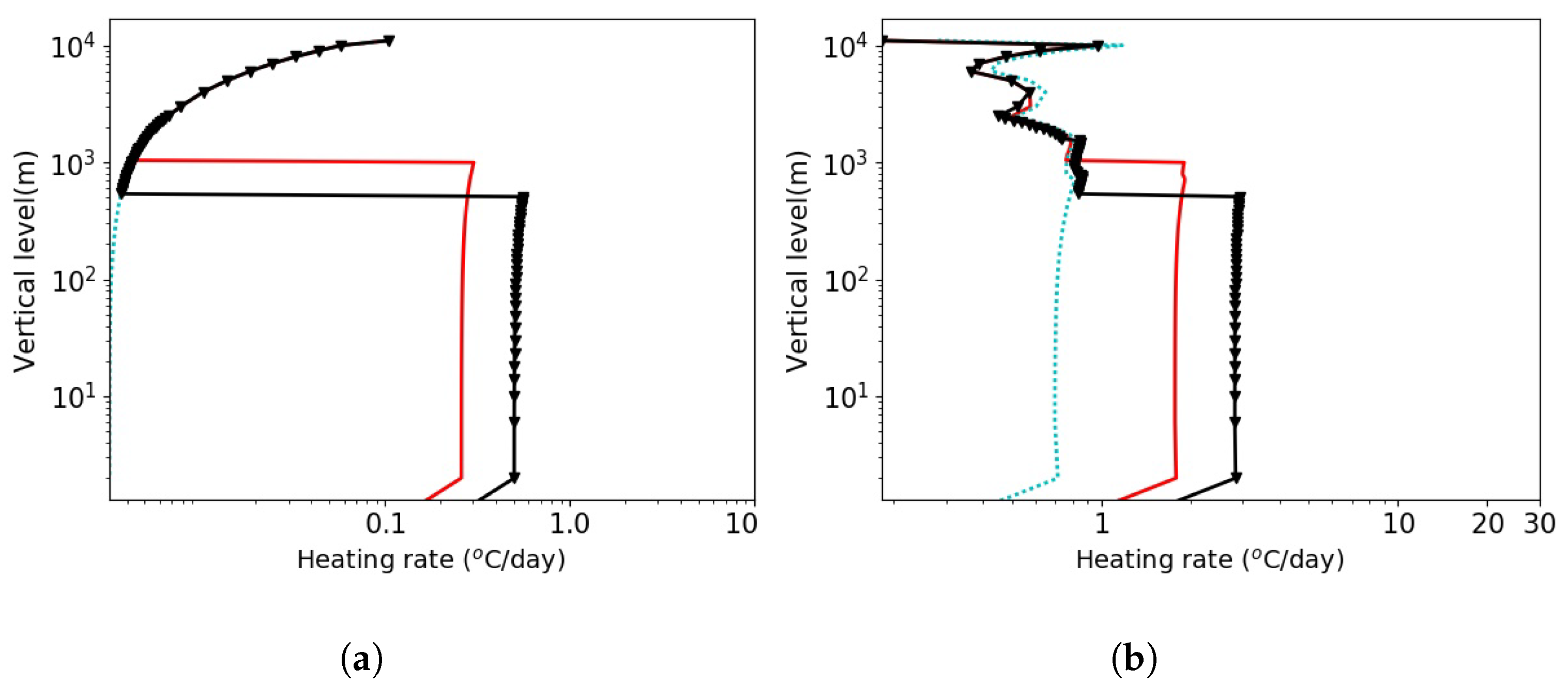
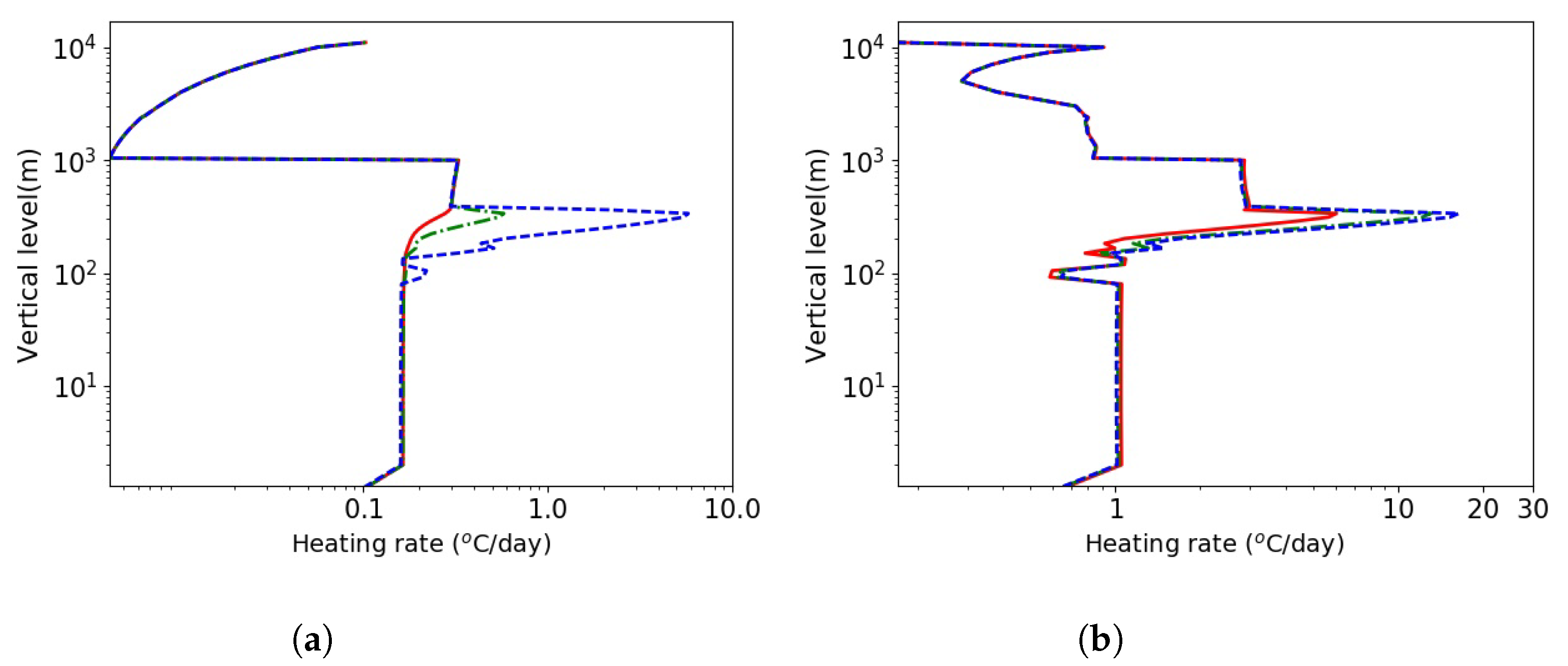
In Section 3, the solar scheme is used and compared to the LH74 scheme for a one-dimensional simulation of a fog event during the ParisFog campaign at SIRTA. The role of aerosols on the heating of atmospheric layers is investigated for clear sky and foggy sky.
3.
In Section 4, sensitivity tests are conducted in order to evaluate the impact of different parametrizations including the presence of aerosols before fog formation, BC in cloud droplets and cloud fraction during and after fog development.

2. The Layer-Dependent Scheme for Solar Radiation in Code_Saturne

The solar radiation scheme proposed by LH74 has been largely used in numerical weather prediction (NWP) for climate modeling and in limited area models (weather research forecast (WRF), [2,16,29,32]) because of its efficiency and its low computer cost. The solar spectrum is divided into two bands: the UltraViolet-visible (UV-vis) band (0.2–0.7 µm) where absorption by ozone occurs in the upper layers of the atmosphere, and the Solar Infrared (SIR) domain (0.7–5 µm) where absorption by water is dominant in the lower part of the atmosphere. The solar radiation scheme of code_saturne is inspired by the LH74 scheme; it has been modified by [2,16] to accurately consider aerosols and cloud fraction in the simulation of direct and global solar radiation at the ground. The major differences between [2,16] are explained in detail in [16]. They concern mainly the calculation of direct irradiance where, in [2], the parameterization of [33] is used while [16] uses a formula for direct radiation derived from LH74 (refer to Section 3.4.5). It has also been used by [29] (XZ14) to model the solar radiation for the different vertical layers of the atmosphere, using a previous version of the solar radiation scheme and making the approximation that aerosols are purely scattering particles.
Here, the solar radiation scheme of code_saturne is modified to model the solar radiation for the different vertical layers of the atmosphere, taking into account the absorbing and scattering properties of particles. They are characterized by their optical properties: aerosol optical depth (AOD), single scattering albedo (SSA) and asymmetry factor. Furthermore, compared to XZ14, maximum and random overlap parameterizations for cloud fraction have been introduced, the adding method for scattering has been added in the UV-vis band, and, following [16], other improvements have been made: the optical air mass, the absorption by minor gases, the Rayleigh diffusion, the choice of the δ two-stream approximation and the estimation of direct radiation that could be important for photovoltaic applications.
The equations are detailed in the appendix (Appendix A for the cloud and aerosol optical properties and Appendix B for the calculation of irradiance fluxes).
At the earth surface, this solar radiative model (part of code_saturneV7.0) has been validated in [16] when considering the atmosphere as being made of one single homogeneous layer, by comparison with irradiance measurements at SIRTA during the year 2014. The results were satisfactory and reported in Table 1.
In order to evaluate the heating of atmospheric layers by solar radiation, a simulation of a fog event is performed in this study using the CFD software code_saturne V7.0 (which includes this solar radiative scheme) during one of the Intensive Observation Periods (IOP) of the ParisFog campaign [30].

3. The ParisFog Experiment

3.1. Observations and Simulation Conditions

Data and simulations used in this study are those of the (IOP)13 of the campaign ParisFog which took place at SIRTA observatory (Palaiseau, France) the 18 and 19 February 2007.
During this IOP, different instruments have been deployed:
  • Vertical profiles of wind, temperature and humidity by radiosondes at 12, 21 (UTC) on the 18 of February and 0000, 0300, 0600, 1000 (UTC) on the 19 of February.
  • Near surface measurements on a 30 m mast of: temperature, humidity, wind and turbulence by sonic anemometers, long wave and solar radiative fluxes.
  • Surface measurements at 2 m of: temperature, humidity, visibility, and radiative fluxes.
  • Fog droplet number with an optical particle counter (OPC) Pallas Wallas 2000.
  • Ceilometer measurements to estimate the fog/stratus layer depth/elevation.
  • Aerosols size distribution with a Scanning Mobility Particle Size (SMPS), an optical particle counter (OPC Grimm 1.109), and filter sampling to determine their chemical composition.
The fog event is simulated here with the one-dimensional atmospheric module of code_saturne described in the previous section, using the same configuration as XZ14. In code_saturne, the prognostic variables evolving in time and on the vertical are: the liquid potential temperature, the horizontal wind components, the total water content (liquid and vapour) and the cloud droplet number concentration. The surface temperature and humidity are imposed at the earth surface. They are computed by an extrapolation method based on the Monin Obukhov similarity theory, where surface temperature and humidity are estimated from their measurements at 2 m and 10 m [34]. The size distribution of fog droplets is described by a log-normal law, and the nucleation scheme of [20] is used. The liquid water content and the partial cloudiness are estimated by using a sub-grid condensation scheme, depending on the sub-grid distribution law for total water content and liquid potential temperature fluctuations [35].
There are several differences compared to the simulations performed by XZ14. First, we use here a more recent version (V7.0) of code_saturne, in which some improvements have been made concerning the turbulent closure of the code. The first-order turbulence closure using a mixing length depending on Richardson number [36] is replaced by the k- ϵ model of version 7.0 [37]. Second, the solar scheme described in the previous section is used, and the influence on the fog evolution of different options related to solar radiations is studied. In XZ14, the optical properties of aerosol are treated as cloud droplets for aerosol optical depth (AOD) but with different climatic values for single scattering albedo and asymmetry factor. The aerosol concentration was considered in the whole atmosphere with a constant value adjusted to minimize the difference between observed and simulated global irradiance at the earth surface. In this study, the total AOD and asymmetry factor are now computed in both the UV-vis and SIR bands using the AERONET data (Data v2.0, level 2.0 at Palaiseau station on 18/02/2007). In fact, the integration over frequency is made following [2] with measurement at 500, 700 and 1400 nm by means of the Angström coefficient due to a lack of experimental knowledge. Aerosols are distributed homogeneously on the vertical into two layers: a first layer of 1000 m depth where 90% of the total AOD is considered and a second layer between 1000 and 3000 m for residual AOD (10% of the total AOD). These altitudes have been chosen in regard to the evolution of the height of the boundary layer during the IOP13 deduced from the vertical profiles of humidity and temperature. The aerosol assymetry factor and single scattering albedo are integrated on the vertical and considered to be constant in time for the duration of the simulation; they are respectively equal to 0.6638 and 0.963 in the UV-vis band and to 0.6486 and 0.964 in the SIR band.
The nucleation scheme of [20], which is used in XZ14, assumes that the aerosol size distribution is made of three lognormal modes, and it takes into account the aerosol chemical composition including the BC fraction. The parameters of these log-normal modes have been deduced from SMPS and OPC measurements by [38] and are used in XZ14. They are shown in Table 2. The chemical composition inferred the critical supersaturation for each mode through an hygroscopicity parameter, which depends on the osmotic coefficient, the fraction of soluble substance, the number of ions produced by dissociation of a salt molecule in water and the molecular weight of the aerosol material. BC is considered as insoluble with an osmotic coefficient of 1. Knowing that cloud condensation nuclei are essentially formed by the accumulation mode (mode 3—Table 2), it is possible to estimate the volume fraction ν d of BC in cloud droplets. As BC in aerosols is determined by filter sampling and chemical analysis, it is necessary to determine the mean wet diameter of mode 3. By using the simple formulation of [39] for the ratio d w e t / d d r y and with a humidity of 95%, we obtain a BC volume fraction of ν d of 8.6 × 10 6 for a concentration of BC of 16% (XZ14) of the dry-aerosol mass in mode 3. This percentage is considered to be constant for the three modes. Then, the maximum possible value is obtained by considering d w e t / d d r y = 1, which leads to ν d = 1.6 × 10 4 .
In the XZ14 simulations using the LH74 scheme, the single scattering albedo and the asymmetry factor for clouds were constant in time and on the vertical. They are now dependent on the equivalent radius of fog droplet, which is variable in time and on the vertical and different in the UV-vis and SIR bands.
In Section 3.2, the fog evolution is simulated with these new conditions with surface temperature and humidity deduced from observation, with random overlap for partial cloudiness and without taking into account BC in cloud droplets (simulation referred to as the ‘base case’ or control simulation).

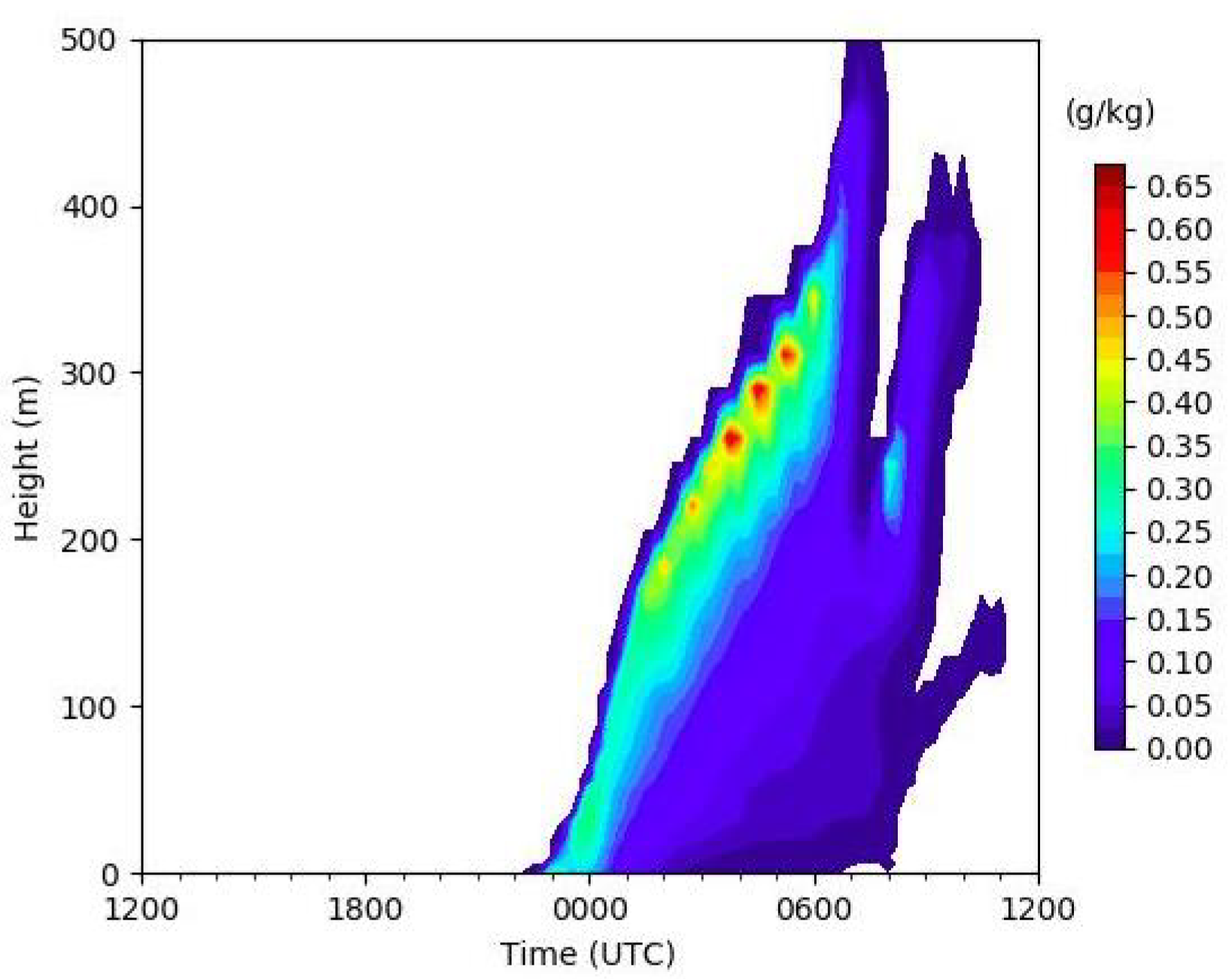
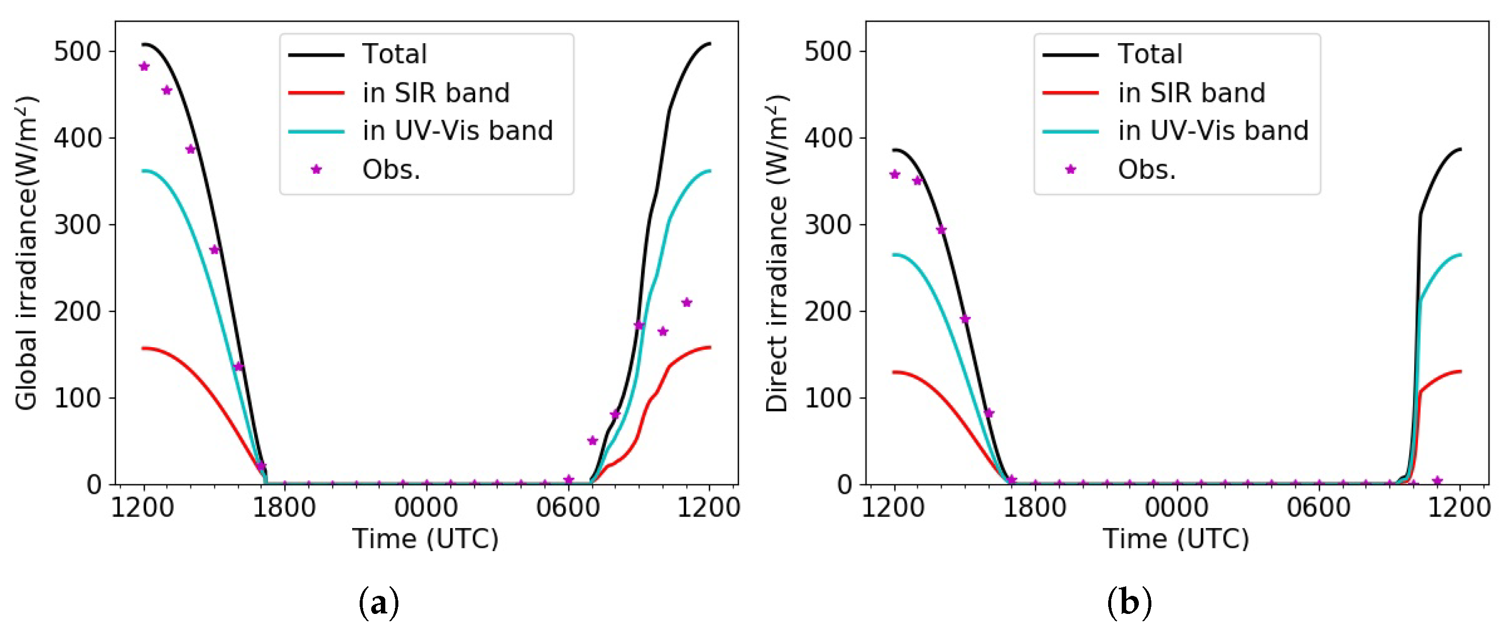
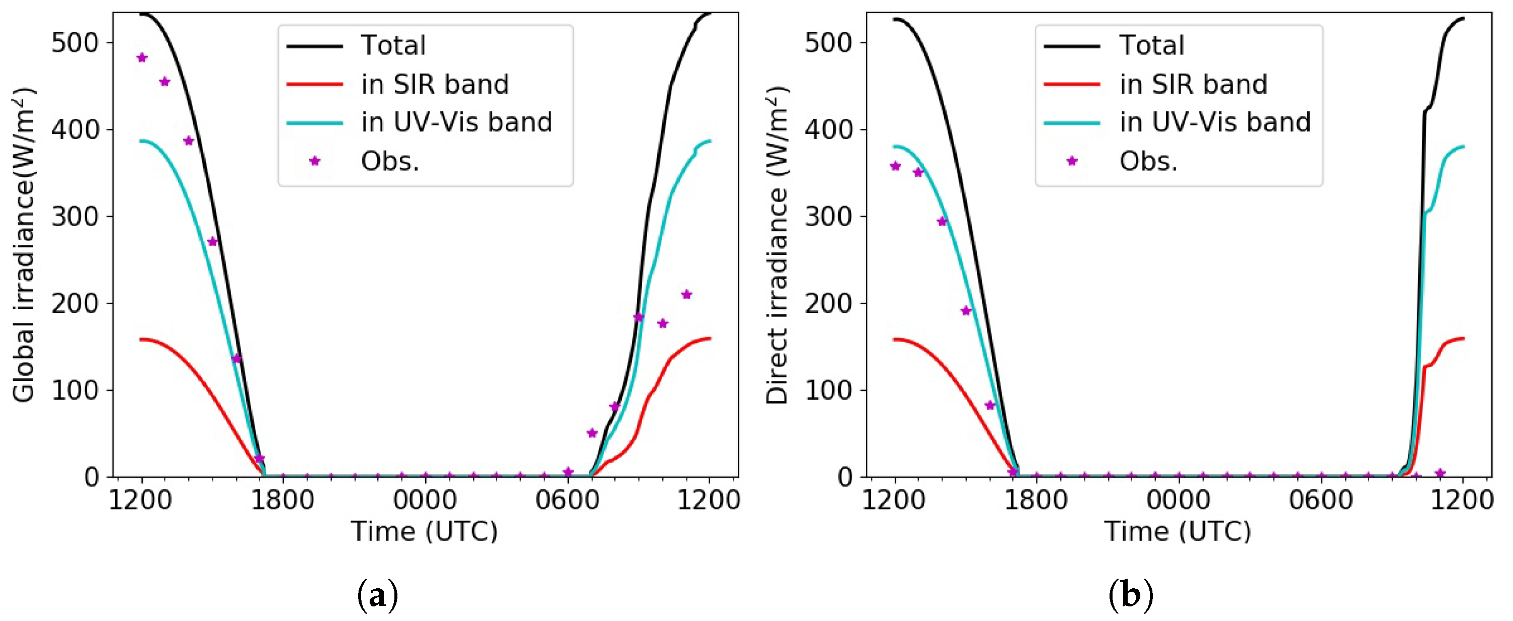
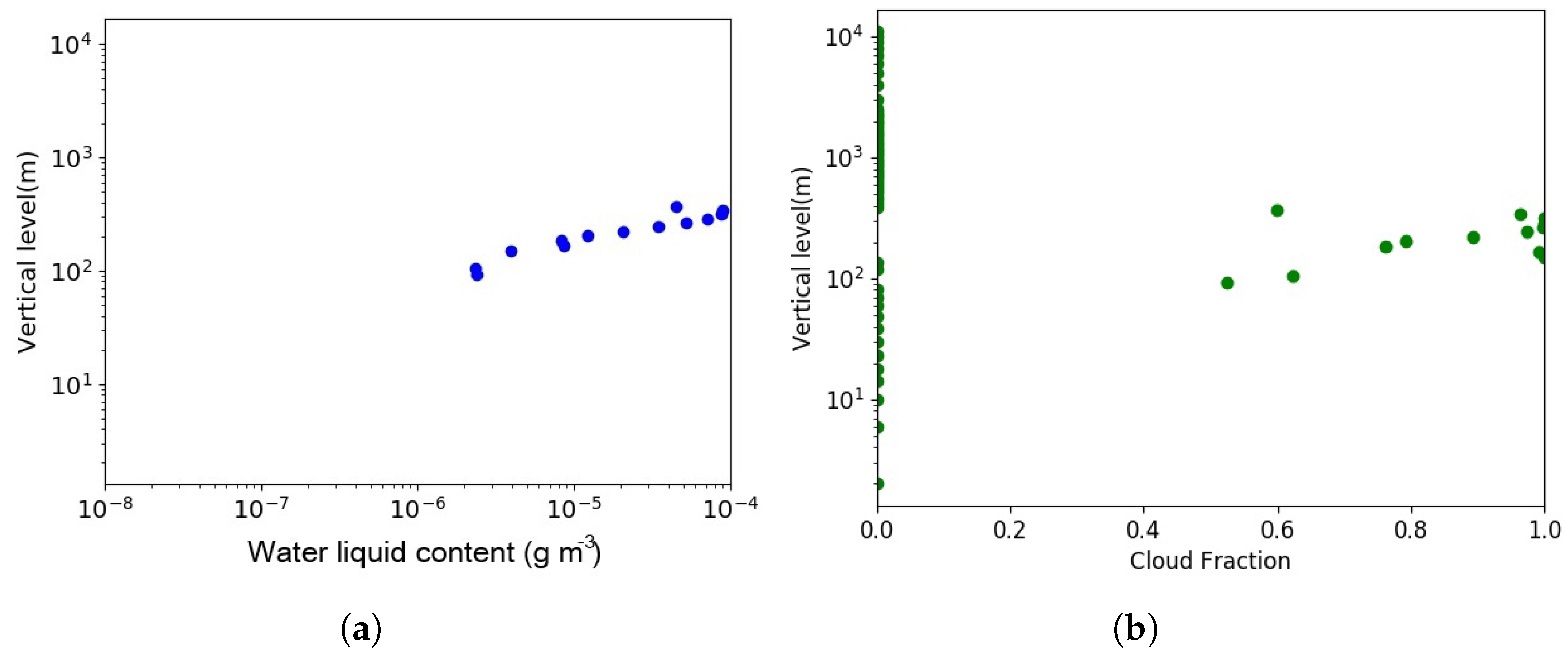
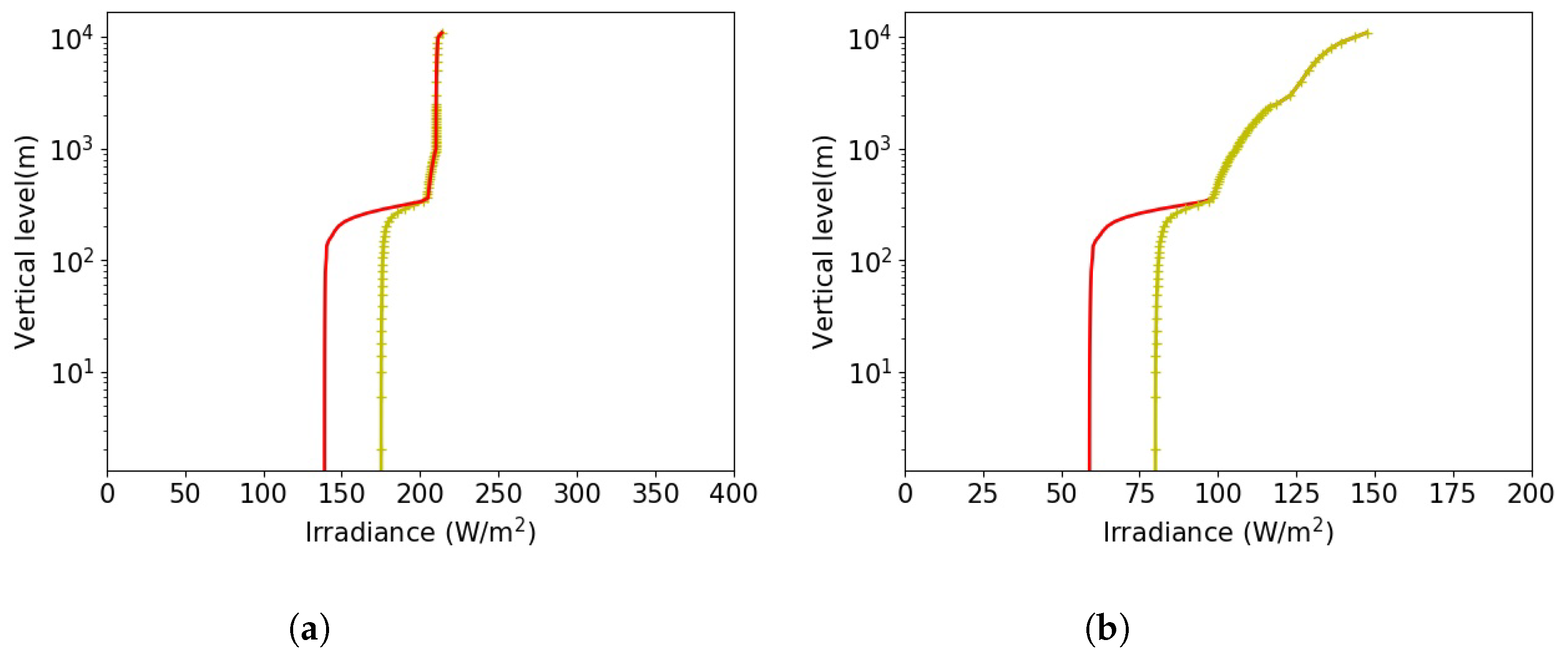
3.2. Fog-Event Simulation

During the IOP13, the fog appears on the 18 of February at 2230 (UTC) after a clear-sky afternoon and dissipates in a low stratus in the morning of the 19 of February at sunrise around 0700 (UTC). This is well represented in the simulation (as seen in Figure 1). Further details about the conditions of this IOP are given in XZ14. Here, we essentially focus on solar radiation effects during the clear-sky phase and the dissipation phase.
On the 18th at 1200 (UTC), the sky is slightly covered with high clouds and becomes more clear in the afternoon. As high clouds are not simulated in the model, the simulated direct solar irradiance is overestimated at 1200 (UTC) compared to observation (Figure 2b). The global and direct irradiances are well estimated by simulation during the afternoon preceding the fog appearance.
Although the influence of aerosols on downward and upward fluxes is taken into account for both UV-vis and SIR bands, the heating rate in clear sky is largely dominated by the SIR band (Figure 3).
During the dissipation phase in the morning of the 19 February, the simulated global irradiance at the surface (Figure 2) compares well to observations between 0600 (UTC) and 0900 (UTC). The stratus disappearance is too fast in the simulation, leading to a large overestimation of both the direct and global irradiances between 1000 (UTC) and 1200 (UTC). Note that during the elevation phase (0600–0900 (UTC)), the stratus is sufficiently deep to totally extinct the observed direct radiation.

3.3. Sensitivity Tests on Aerosols

The fog evolution is impacted by aerosols in different ways: first, aerosols directly impact the irradiance fluxes and the heating rates, but also, they impact the nucleation into cloud droplets and the chemical composition of the droplets. Here, their influence on the fog evolution through the irradiance fluxes is studied by performing a simulation without taking into account aerosols in the modeling of the irradiance fluxes. This impact is presented in Figure 4 for the irradiance fluxes at the earth surface and in Figure 3 for the vertical distribution of the heating in the atmospheric layers at 1500 (UTC). The temporal evolution of the simulated liquid water content is similar to the one of the base case (Figure 1). Therefore, the dissipation of the fog is not much affected by considering aerosols in the modeling of solar radiation fluxes here. In fact, as surface temperature and humidity are forced observations in all the simulations of this paper, the contribution of aerosols is only taken into account in the heating rate of the atmospheric layers, which is insufficient to significantly modify the evolution of the fog layer in the dissipation phase. Nevertheless, the surface solar irradiances (Figure 4), as expected, are largely overestimated if aerosols are not considered. The gap at 1200 (UTC) is around 30 W m 2 for the global and 150 W m 2 for the direct. The larger overestimation of the direct component is linked to the scattering of aerosols, which transform direct irradiation to diffuse irradiation. Note the very weak differences between global and direct irradiances for the simulation without aerosols. This is due to Rayleigh diffusion, which is only parameterized in the UV-vis band by means of the factor 1/(1 − R a ¯ R g ) as in LH74 ( R a ¯ and R g are defined in Appendix B). Compared to the control simulation, the heating in the layers is very low in the UV-vis band (corresponding to ozone absorption) if aerosols are not considered in the modeling of the irradiances; in the SIR band, it decreases approximately 0.9 °C/day.
Because the exact distribution of aerosols on the vertical is unknown due to the time variability of the boundary layer height during the IOP13, it is interesting to estimate the effect of a more concentrated aerosol layer in the lower part of the atmosphere which is equivalent to a lower boundary layer height. This could represent a pollution event as it often appears during winter anticyclones, which are favorable to radiation fogs. The heating rate for a simulation with a depth of 500 m for the first aerosol layer close to the ground instead of 1000 m is presented in Figure 3. The heating rates increase strongly from 1.8 to 2.8 °C/day in the SIR band and from 0.25 to 0.5 °C/day in the UV-vis band. In that case, the contribution of UV-vis band to heating rate is not negligible compared to that of the SIR band.
Note that aerosol properties are estimated from AERONET data. The role of BC concentration in aerosol particle as studied in [19] is not investigated in this paper, which rather focuses on the influence of the fraction of BC in cloud droplets on the fog evolution.

3.4. Sensitivity Tests on the Fog Evolution

Sensitivity tests are conducted in order to evaluate the impact of a better description of cloud optical properties in the solar irradiance scheme. Here, we are specifically interested in the solar heating in the cloud layers. In this paragraph, the results are presented at 0900 (UTC) before the disappearance of the stratus and when solar heating is significant. The vertical profile of liquid water content and cloud fraction are presented in Figure 5 for the base case. Firstly, each sensitivity simulation is performed by modifying a particular variable, such as the cloud optical depth. The same vertical profiles of liquid water content and cloud fraction as in the base case are used. They are shown in Figure 5. This set of sensitivity simulations are referred to as the ‘stationary’ tests. Then, the impact of the modification of the variable on the simulated fog is evaluated by letting the liquid water path and cloud fraction evolve accordingly to this change. This set of sensitivity simulations are referred to as the ‘evolving’ tests. The ‘evolving’ tests help understand the impact of the modified variables on the liquid water field and how it affects the results of simulations and the dissipation of the fog.

3.4.1. Sensitivity to Interstitial Aerosols

Interstitial aerosol particles are particles that are too small to be activated to cloud droplets. However, for rigorous calculations, they should be considered during cloudy-sky situations. This is done by adding the AOD to the COD during cloudy-sky situations in Equations (A6)–(A8) and in the estimation of the direct irradiance for the base case. However, not taking into account interstitial aerosols in the cloud layer of our simulation has a very low impact both on the heating rate and fluxes. For the ‘stationary’ test, the heating rate at the top of the cloud layer decreases by less than 0.3 °C/day in the UV-vis band and 0.2 °C/day in the SIR band. Similarly, the downward global and direct surface irradiances are slightly impacted, with an increase lower than 1.4 W m 2 in the UV-vis band and 0.35 W m 2 in the SIR band. Interstitial aerosols do not impact the evolution of the cloud layer during its dissipation phase.

3.4.2. Sensitivity to Effective Radius of Cloud Droplet

The effective radius of cloud droplets is used for the calculation of the SSA and asymmetry factor (equations in Appendix A). It is variable in time and space, and the average radius is equal to 2.7 μ m (the average has been calculated for all cloudy layers, in time and on the vertical). Taking the constant value of 2.7 μ m in the model has a very low impact both on the heating rate (less than 0.5 °C/day) and irradiance fluxes (less than 1 W m 2 ). However, a constant effective radius of 10 μ m, often used as a climatological value for low clouds, increases both the global and direct irradiances. Compared to the base case in the stationary case at 0900 (UTC), the heating rate is mainly impacted in the SIR band with an increase of 1.9 °C/day. The downward surface irradiance is strongly impacted, it is higher by approximately 36 W m 2 in the UV-vis band and 22 W m 2 in the SIR band (Figure 6). An overestimation of the droplet radius reduces the value of the cloud optical depth, which increases the downward fluxes under the cloud. In the UV-vis band, the scattering to space is now lower; in the SIR band, the absorption in the cloud layer is lower. As the impact on the heating rate is relatively low and as the earth surface temperature is forced to observation in our simulations, the dissipation of the fog is not impacted by these variations of the effective radius of cloud droplets.

3.4.3. Sensitivity to BC Concentration

In the base case, the influence of the BC concentration in the cloud droplet on the heating rate is not considered. However, BC absorbs solar irradiation and increases the heating rate in the atmospheric layers. The BC concentration can be taken into account in the calculation of the SSA of clouds following [22] (refer to Appendix A for equations). We do not have direct measurements of the BC fraction in the fog droplet and large uncertainty on aerosol wet diameter; therefore, we consider two possible BC fractions in cloud droplets: V f B C = 8.6 × 10 6 and the maximum value of V f B C = 1.6 × 10 4 , as detailed in Section 3.1.
The introduction of BC with V f B C = 8.6 × 10 6 in cloud droplets impacts the heating rate (Figure 7) and fluxes at the ground. In the ‘stationary’ test, as expected, the heating rate is accentuated at the top of the cloud layer where the liquid water content is maximum. There is an increase of the heating rate of approximately 7 °C/day in the SIR band and 0.3 °C/day in the UV-vis band at 0900 (UTC). In that case, the contribution of the UV-vis band to the heating rate becomes significant. As absorption of irradiance is more important in the cloud layers, the global and direct irradiances at the earth’s surface are directly impacted by taking into account BC concentration in the cloud droplet. However, this impact is weak: at 0900 (UTC), compared to the base case, the global irradiance is lower than −1.45 W m 2 in the SIR band and −0.22 W m 2 in the UV-vis band. In the ‘evolving’ test, the total heating rate is higher (by 3.2 °C/day) when the BC fraction in cloud droplets is taken into account, and the global irradiances at the earth’s surface increase by 9.2 W m 2 in the SIR band and 18.4 W m 2 in the UV-vis band at 0900(UTC) compared to the base case (figures not presented here).
When V f B C is equal to 1.6 × 10 4 , as expected, the heating in the layers increases even more: compared to the base case, there is an increase of approximately 5.5 °C/day in the UV-vis band and 10.3 °C/day in the SIR band for the ‘stationary case’ (Figure 7). That leads to a decrease of the global irradiance at the earth’s surface of −2 W m 2 in the SIR band and −4 W m 2 in UV-vis band compared to the base case. For the ‘evolving’ test, the water liquid content is impacted and is reduced (by around 0.05 g/kg) during and after the dissipation of the fog compared to the base case. The fog elevates from the ground earlier (around 0600 (UTC) instead of 0700 (UTC)), and the stratus cloud dissipates faster (the stratus now is completely dissipated around 0930 (UTC) instead of 1100 (UTC)). That corresponds to a significant increase of the surface irradiances, at 0900 (UTC) for global irradiance (+6.0 W m 2 in the SIR band, +28.8 W m 2 in the UV-vis band) and at 1000 (UTC) for direct irradiance (+39.4 W m 2 in the SIR band, +77.4 W m 2 in the UV-vis band).

3.4.4. Sensitivity to the Treatment of Partial Cloudiness

In this study, the evolution of a fog layer that elevates in a stratus at the end of the morning is simulated. For these conditions, as mentioned by Tian and Curry (1989), it seems more appropriate to assume maximum overlapping instead of random overlapping for the partial cloudiness. Even though the heating rate does not change significantly when assuming random overlapping (+1.1 °C/day in the SIR band), the upward and downward fluxes are impacted both in the UV-vis and SIR bands, leading to a slight decrease of solar irradiances at the earth’s surface (−3.3 W m 2 in the SIR band, −5.6 W m 2 in the UV-vis band). The evolution of the fog layer is not modified, the cloud fraction being equal to 1 in the cloud layer from 0600 (UTC) to 0800 (UTC). The cloud fraction only differs from 1 in the dissipation phase after 0900 (UTC) when the liquid water content in the cloud layer is very low.

3.4.5. Simplified Parametrization

As shown in the sensitivity study, the solar heating in the lower part of the atmosphere is low in the UV-vis band compared to the SIR band. In fact, ozone absorption is only efficient in the upper layer of the atmosphere, and overlap correction between gas and particles can be neglected in the troposphere. In addition, the spatial and time variability of effective radius is not very important if a correct averaged value is used for the cloud droplet. Here, a simpler parameterization of solar heating in the UV-vis band is designed in order to save computer cost. In addition, for many applications, only the global and direct solar fluxes at the earth’s surface are necessary, and the vertical distribution of fluxes is not useful. Considering the integral cloud and aerosol optical properties, as in [2,16], the downward fluxes at the ground surface in the UV-vis band can be written as:
F g U V - v i s , n c = μ 0 F ( 0.647 A o 3 ( x ) R r ¯ ( μ 0 ) ) T m g T a / ( 1 R a R g )
F g U V - v i s , c = μ 0 F ( 0.647 A o 3 ( x ) R r ¯ ( μ 0 ) ) T m g T c / ( 1 R c R g )
F d U V - v i s , n c = μ 0 F ( 0.647 A o 3 ( x ) R r ¯ ( μ 0 ) ) T m g e m τ a t o t
F d U V - v i s , c = μ 0 F ( 0.647 A o 3 ( x ) R r ¯ ( μ 0 ) ) T m g e m τ c t o t
With x = mu O 3 (, 0), T a , R a , T c , and R c are calculated as Equations (A12) and (A13) but for the total optical depth of cloud τ c t o t and aerosol τ a t o t , the different variables are defined in Appendix B.
The heating rate in the layers is computed as in LH74 with Equations (A33)–(A35) and (A43). The simplification of the parameterization consists in neglecting absorption in the aerosol and cloud layers that are considered as purely scattering in the UV-vis band. In the stationary test at 0900 (UTC), the difference with the base case is low, 0.22 °C/day in the SIR band and −0.32 °C/day in the UV-vis band where there is no heating rate due to aerosols. The results of this simpler parameterization for the surface irradiances at 0900 (UTC) for the UV-vis band (compared to the base case, the difference for the global: 1.3 W m 2 ; direct: 0.07 W m 2 ) and SIR band (compared to the base case, the difference for the global: −0.19 W m 2 ; direct 0 W m 2 ) are quite similar to the base case. For the ‘evolving’ test, as the total heating rate (sum of UV-vis band and SIR band contributions) is very close to that of the base case, the liquid water content in the fog/stratus layer is similar and the differences for surface irradiances are low: for example, at 0900 (UTC), in the UV-vis band, the actual version differs for the base case by +1.23 W m 2 for the surface global irradiance and by +0.05 W m 2 for the surface direct irradiance; in the SIR band, the differences are equal to +0.4 W m 2 for surface global irradiance and 0 W m 2 for surface direct irradiance. The dissipation of the fog is not affected. Calculations are simpler, which shows the advantage of using such a method that is a good first approximation. Note that if the corrections of Joseph et al. (1976) are omitted when using this simplified method, code_saturne results are not impacted for this specific case.

4. Conclusions

A simple solar radiation scheme has been developed in order to introduce the aerosols in the two-stream parameterization of Lacis and Hansen, (1974). Two spectral bands are considered: the UV-vis band (0.2–0.7 μ m) where ozone absorption is predominant in the stratosphere and the SIR band (0.7–5 μ m) where absorption and diffusion by water vapor, clouds, aerosols and Rayleigh scattering are the major processes in the troposphere.
Substantial improvements have been introduced to the original version.
The optical properties of clouds (optical depth, single scattering albedo and asymmetry factor) are now taken into account in both spectral bands, and they are estimated as functions of the effective radius of the cloud droplet. The optical properties of aerosols are also differentiated for each band. In order to include clouds and aerosols effects in the UV-vis band, the adding method is introduced to calculate transmission and reflection functions for clouds and aerosols layers as for the SIR band but by neglecting the overlapping with ozone in the lower atmosphere. The two-stream method has been modified to take into account highly forward scattering due to cloud droplets and aerosols following Joseph et al. (1976) for both quadrature and standard Eddington approximations with a re-actualized optical air mass formulation. The cloud fraction has been introduced in the solar scheme, giving us the possibility to use random or maximum overlapping for the different cloud layers. For photovoltaic application, the downward direct solar irradiance is now computed and absorption by minor atmospheric gases such as CO 2 , CO, N 2 O, CH 4 , and O 2 has been added in the global and direct vertical fluxes. This solar scheme has been used to simulate a case of fog event during the ParisFog campaign. The effect of the main improvements has been illustrated. Note that this study of processes is applicable to the 2007 ParisFog experiment conditions/parameters. However, in a more recent case study, the results may change based on climatological changes in the past decade. The main conclusions are:
As expected, before the fog formation (clear-sky conditions), aerosols play a major role in the estimation of radiation and heating rates. When they are not considered, the fluxes at the surface are highly overestimated (especially, the direct flux that increases of 150 W m 2 ), and the heating in the layers is strongly underestimated both in the UV-vis and SIR bands (decrease of 0.9 °C/day in the SIR band) compared to the base case in which a 1000 m deep aerosol layer is introduced. For the lower aerosol boundary layer (higher concentration of aerosols in the low atmosphere), as a representation of a pollution event in winter time, the heating in this layer increases, especially in the UV-vis band: it increases by 55% in the SIR band and 100% in the UV-Vis band. The aerosol absorption becomes significant compared to the SIR band: the heating rate in the UV-vis band is now approximately 30% of the heating rate in the SIR band.
During the fog dissipation, considering the BC concentration in the cloud droplets modifies sensitively the distribution of heating rate in the vertical. The total heating rate increases at the top of the cloud layer by 7.3 °C/day for BC volume fraction in cloud droplets of 8.6 × 10 6 and by 15.8 °C/day for a BC volume fraction in cloud droplets of 1.6 × 10 4 . Even if this effect is rather low with a BC concentration fraction in cloud droplets of 8.6 × 10 6 , it might be major for more persistent clouds or fog in low atmosphere. Concerning the impact of the cloud microphysics on solar heating, it seems that a constant value for the effective radii of the cloud droplet is a good approximation if the mean value retained is well adapted for the type of cloud simulated. In our simulations, we assume that the maximum overlapping instead of the random overlapping has a very low impact on the cloud fraction and that the cloud fraction is close to 1 when the fog/stratus water content is significant. In that case, the random overlapping assumption has the advantage of being more economic in computer cost. Lastly, in order to save computational cost in solar radiation calculations, neglecting the solar heating in the UV-vis band in the lower part of the atmosphere is indeed a good first approximation as underlined by the work of LH74 if aerosols and clouds are correctly considered in the estimation of downward solar fluxes at the ground surface.

Author Contributions

Conceptualization, L.M.-G. and L.A.A.; methodology, L.M.-G.; software, M.F.; validation, E.D., K.S., L.M.-G. and M.F.; formal analysis, L.A.A. and L.M.-G.; investigation, L.A.A.; writing—original draft preparation, L.M.-G. and L.A.A.; writing—review and editing, E.D., K.S. and M.F.; supervision, E.D. and K.S. All authors have read and agreed to the published version of the manuscript.

Funding

The work of A.-A.L. was supported by CEREA, a member of the Pierre-Simon Laplace Institute (IPSL) and by ANRT through an EDF-CIFRE contract (Grant number: 2018/1415).

Institutional Review Board Statement

Not applicable.

Informed Consent Statement

Not applicable.

Acknowledgments

The authors would like to acknowledge SIRTA for providing the data used in this study.

Conflicts of Interest

The authors declare no conflict of interest.

Appendix A. Optical Characteristics of Aerosols and Clouds

Both cloud droplets and aerosols induce scattering. They are characterized by their optical properties, their optical thicknesses τ c and τ a , their SSA ω c and ω a and their asymmetry factor g c and g a .
For clouds, the optical parameters τ c , ω c , g c depend on the equivalent cloud droplet’s radius r e (in μ m) following [40]:
τ c = 3 2 L w c r e
where L w c is the liquid water content in g m 2 .
Following [41], the expressions of ω c and g c are wavelength dependent. They are defined for the SIR band and for the UV-vis band separately. The integration over wavelengths for the UV-vis and SIR bands is done by weighting each wavelength band Δ λ i with the radiance energy E ( Δ λ i ) in the band following [16,42,43]:
ω c = i = 1 α ω Δ λ i E ( Δ λ i ) i = 1 α E ( Δ λ i )
g c = i = 1 α ω Δ λ i g Δ λ i E ( Δ λ i ) i = 1 α ω Δ λ i E ( Δ λ i )
where Δ λ represents the wavelength difference of each spectral band of the UV-vis or the SIR domain. The UV-vis domain is divided into α = 2 spectral bands: 250–440 nm; 440–690 nm (represented by the indicator ‘i’). The near SIR domain is also divided into α = 2 spectral bands: 690–1190 nm; 1190–2380 nm (represented by the indicator ‘i’).
The SSA ω c as calculated above is used in the case where BC concentration is neglected in the cloud droplet (volume fraction of BC in cloud droplet is lower than 1 × 10 8 ). In the other case, BC concentration is taken into account following [22]. They developed a parametrization to calculate the SSA in function of the mean cloud droplet diameter and the volume fraction of BC in the cloud droplet. It is defined for different spectral bands by the following expression:
ω ¯ ( ν d , d o ) = ω c ¯ + β 1 ( 1 e β 3 ( ν d ν o ) ) + β 2 ( 1 e β 4 ( ν d ν o ) )
For a cloud droplet diameter d o = 20 μ m, the droplet volume BC fraction ν d is ν o = 10 8 and ω ¯ c = 1 − ω c , the single scattering co-albedo without BC. β i coefficients and ω ¯ c are given in [22] for different spectral bands. The dependence on droplet diameter d is approximated by:
ω ¯ ( ν d , d ) = d d o ω ¯ ( ν d , d o ) 1 + 1.8 ω ¯ ( ν d , d o ) ( d d o 1 )
The integration over both UV-vis and SIR bands is made by weighting the resulting SSA with the radiance energy contained in each band.
For aerosols, the AOD, SSA and asymmetry factors given at a specific wavelength are integrated over the UV-vis and SIR bands. For this specific case, they are constant in time and taken from the AERONET database.

Appendix B. Estimation of Solar Radiation

Appendix B.1. Solar Radiation in the SIR Band

For water droplets, the multiple diffusion processes are directly modeled using the adding method with a k-distribution method for overlapping between liquid and vapour water absorption (LH74).
For each cloud layer l in the frequency interval n, the optical thickness τ l , n , the single scattering albedo ω l , n and the asymmetry factor g are:
τ l , n = τ c + τ a + k n u w v
ω l , n = ( ω c τ c + ω a τ a ) / τ l , n
g = ( ω c τ c g c + ω a τ a g a ) / ( ω l , n τ l , n )
where u w v ( z , z ) = z z ρ h 2 o ( z ) ( P ( z ) P 0 T 0 T ( z ) ) m d z with m = 1 as suggested by LH74.
Ref. [44] corrections are used in order to describe highly forward scattering for cloud droplets and aerosols.
That gives with f = g 2 [40]:
τ l , n = τ l , n ( 1 f ω l , n )
ω l , n = ω l , n ( 1 f ) / ( 1 f ω l , n )
g = ( g f ) / ( 1 f )
The transmission and reflection functions used in the adding method for the two-stream approximation for the solar global radiation are described by [45].
R l = γ 2 ( e k τ e k τ ) ( k + γ 1 ) e k τ + ( k γ 1 ) e k τ
T l = 2 k ( k + γ 1 ) e k τ + ( k γ 1 ) e k τ
with τ = τ l , n and k = ( γ 1 2 γ 2 2 ) 1 / 2 . The values γ 1 and γ 2 depend on the two-stream approximation used:
Standard Eddington approximation (SEA [45,46])
γ 1 = 1 / 4 ( 7 ω l , n ( 4 + 3 g ) )
γ 2 = 1 / 4 ( 1 ω l , n ( 4 3 g ) )
Two-stream quadrature approximation [17,45]
γ 1 = 3 1 / 2 ( 1 ω l , n ( 1 + g ) / 2 )
γ 2 = 3 1 / 2 ω l , n ( 1 g ) / 2 )
With the corrections of [44], these approximations are often called δ two-stream or δ -Eddington [17]. The transmission function for direct solar radiation is T l = e x p ( m ( τ a + k n u w v ) ) for the clear-sky layers and for the cloudy layers, T l = e x p ( m ( τ a + τ c + k n u w v ) ) where m is the optical air mass following [47]:
m = 1 / ( μ 0 + 0.50572 ( 96.07995 ( 180 / π ) × a c o s ( μ 0 ) 1.6364 )
where μ 0 is the azimuth angle. When the random overlapping assumption is considered for cloudiness, the reflection and transmission functions are weighted by cloud fraction C f l , as suggested by [48]: T l = C f l T l c + ( 1 C f l ) T l n c and R l = C f l R l c + ( 1 C f l ) R l n c .
To determine absorption in each vertical layer, the adding method is applied as described in LH74 and summarized below. It considers a discrete probability distribution of water vapor absorption coefficients, as described in Table A1.
Table A1. Discrete probability distribution of water vapor absorption coefficients for n = 1, 8 (LH74).
k n , n ∈ [1, 8]4 × 10 6 2 × 10 6 0.00350.03770.1950.944.4619
p(k n )0.64700.06980.14430.05840.03350.02250.01580.0087
These coefficients are determined in order to have:
A w v ( y ) = 0.29 ( 1 + 14.15 y ) 0.635 + 0.5925 y
for y = u w v in kg m 2 .
The layer transmission and reflection functions going down and going up are added.The upward and downward global fluxes boundary between the layers 1, l and l, L + 1 are determined by (the level L corresponds to the ground level):
For global radiation:
U l = T 1 , l R L + 1 , l 1 R 1 , l R L + 1 , l + 1 ; D l = T 1 , l 1 R 1 , l R L + 1 , l + 1
for direct radiation:
U l d = 0 ; D l d = T 1 , l
with T 1 , 1 = e x p ( m u w v ( 11 , 000 , ) and R 1 , 1 = 0 as an upper boundary condition for both global and direct radiations in order to take into account the absorption by water vapor above 11,000 m and R L + 1 = R g and T L + 1 = 0 at the ground surface where R g is the ground albedo. The fraction of the total incident flux absorbed in the upper composite layer is:
A 1 , l ( n ) = p ( k n ) [ ( 1 R 1 , L + 1 ( n ) ) + U l ( n ) D l ( n ) ]
and the total absorption in each layer l is found by differencing:
A l ( n ) = A 1 , l ( n ) A 1 , l 1 ( n )
The total absorption F a b s S I R and the fluxes F g S I R (global downward), F g S I R (global upward), and direct downward F d S I R in each layer l are found by summing over the values of n:
F a b s S I R = μ 0 F n = 2 n = 8 A l ( n ) ,
F g S I R = μ 0 F n = 2 n = 8 D l ( n ) p ( k n ) ,
F g S I R = μ 0 F n = 2 n = 8 U l ( n ) p ( k n ) ,
F d S I R = μ 0 F n = 2 n = 8 D l d ( n ) p ( k n )
Note that in this adding method, for a homogeneous cloud or aerosol layer: R l = R l and T l = T l where the asterisk indicates illumination from below.
In the case where cloud fraction is taken into account with maximum overlapping, the adding method has to be done for cloudy atmosphere (c) and for atmosphere without clouds (nc) but with aerosols (in that case τ c = 0). The fluxes and the heating rate are weighted by the maximum of the cloud fraction C f m a x encountered between and the ground level L.

Appendix B.2. Solar Radiation in the UV-Vis Band

The multiple diffusion processes are directly modeled with the adding method but without the k-distribution method for ozone absorption, as it is relevant only in the upper layers of the atmosphere. Nevertheless, ozone absorption is taken into account after the adding method computation by adding its contribution to heating rate. The same adding method procedure as water vapor is applied but by keeping only cloud and aerosol optical depth in the transmission and reflection functions. In that case, the boundary conditions at the top of the aerosol/cloud layer are: T 1 , 1 = 1; R 1 , 1 = 0 and at the ground T L + 1 = 0; R L + 1 = R g .
The total absorption only due to aerosols and clouds in each layer l is found as for water vapor by:
F a b s U V v i s = μ 0 F ( 0.647 A O 3 ( x ) R r ( μ 0 ) ) ( A 1 , l A 1 , l 1 )
The downward flux for global and direct radiation and the upward diffuse flux at the ground surface as described in [16] are:
F g U V v i s = μ 0 F ( 0.647 A O 3 ( x ) R r ( μ 0 ) ) D l
F d U V v i s = μ 0 F ( 0.647 A O 3 ( x ) R r ( μ 0 ) ) D l d
F g U V v i s = μ 0 F ( 0.647 A O 3 ( x ) R r ( μ 0 ) ) U l
where A o 3 is the ozone absorption and R r ( μ 0 ) = 0.28 / ( 1 + 6.43 μ 0 ) is the Rayleigh atmospheric albedo. A o 3 is parameterized as LH74 for both Chappuis and ultraviolet bands:
A O 3 = 0.02118 x 1 + 0.042 x + 0.000323 x 2 + 1.082 x ( 1 + 138.6 x ) 0.805 + 0.0658 x 1 + ( 103.6 x ) 3
where x = u o 3 ( z ) is the ozone amount in cm STP above the altitude z given by the well-known analytical function of Green (1964) u o 3 = a ( 1 + e x p ( b / c ) / ( 1 + e x p ( ( z b ) / c ) with a = 0.4 cm STP, b = 20 km and c = 5 km.
In the clear sky layers above the aerosol/cloud layers, the irradiances are computed as LH74, making the hypothesis of a pure absorbing layer on the top of a reflecting region. With this approximation, the solar heating rate due to ozone in the layer ( l , l + 1 ) is (LH74).
Above the aerosol layer when there is no cloud (nc)
F a b s U V v i s , n c = μ 0 F [ A o 3 ( x l + 1 A o 3 ( x l R a n c ¯ A o 3 ( x l + 1 A o 3 ( x l ) ) ]
with x = m u O 3 (, z), x = m u O 3 (, 0) + m ¯ ( u O 3 (, 0) − u O 3 (, z)) where m ¯ = 1.9 is the optical air mass for diffuse irradiance.
R a n c is the composite albedo including aerosol diffusion effect and ground reflectivity,
R a n c = R a ¯ + T a ¯ R g T a ¯ / ( 1 R a ¯ R g )
where T a ¯ and R a ¯ are calculated with Equations (A13) and (A12) for the total optical aerosol depth τ a t o t .
Above the aerosol/cloud layer in cloudy conditions (c):
F a b s U V v i s , c = μ 0 F [ A o 3 ( x l + 1 A o 3 ( x l R c c ¯ A o 3 ( x l + 1 A o 3 ( x l ) ) ]
R c c is determined as R c n c with Equations (A13) and (A12) but for the total optical cloud depth τ c t o t
R c c = R c ¯ + T c ¯ R g T c ¯ / ( 1 R c ¯ R g )
The global and direct downward irradiances are equal for both cloud and no cloud situations:
F g U V - v i s = F u U V v i s = μ 0 F ( 0.647 A o 3 ( x ) R r ( μ 0 ) )
The upward irradiance:
F g U V - v i s , n c = μ 0 F ( 0.647 A o 3 ( x ) R r ( μ 0 ) ) ( R a ¯ + U t o p )
F g U V - v i s , c = μ 0 F ( 0.647 A o 3 ( x ) R r ( μ 0 ) ) ( R c ¯ + U t o p )
where U t o p is the fraction of the upward flux at the top of the aerosol/cloud layer coming from the reflection by the earth surface through the aerosol/cloud layers. When a maximum overlapping assumption is made for cloud fraction, as for the SIR band, the fluxes and the heating rate are weighted by the maximum of the cloud fraction C f m a x .
F g U V - v i s = C f m a x F c g U V - v i s + ( 1 C f m a x ) F n c g U V - v i s
F d U V - v i s = C f m a x F c d U V - v i s + ( 1 C f m a x ) F n c d U V - v i s
F g U V - v i s = C f m a x F c g U V - v i s + ( 1 C f m a x ) F n c g U V - v i s
F a b s U V - v i s = C f m a x F a b s U V - v i s , c + ( 1 C f m a x ) F a b s U V - v i s , n c

Appendix B.3. Total Solar Radiation

The fluxes for global and direct radiations are the sum of the contribution of both UV-vis and SIR bands but multiplied by T m g in order to consider the absorption by minor gases. The general transmittance function, T i , for five minor atmospheric gases (CO 2 , CO, N 2 O, CH 4 and O 2 ) is expressed by the following equation [12]:
T i = 1 a m u i / ( ( 1 + b m u i ) c + d m u i )
where m is the optical air mass, and a , b , c , d are numerical coefficients that are given in the table given by [12].
The broadband transmittance function due to the total absorption by the uniformly mixed gases is then calculated by:
T m g = T C O 2 T C O T N 2 O T C H 4 T O 2
The downward fluxes are equal to:
Global radiation
F g = T m g ( F g U V - v i s + F g S I R )
Direct radiation
F d = T m g ( F d U V - v i s + F d S I R )

References

  1. Rap, A.; Scott, C.E.; Spracklen, D.V.; Bellouin, N.; Forster, P.M.; Carslaw, K.S.; Schmidt, A.; Mann, G. Natural aerosol direct and indirect radiative effects. Geophys. Res. Lett. 2013, 40, 3297–3301. [Google Scholar] [CrossRef] [Green Version]
  2. Sartelet, K.; Legorgeu, C.; Lugon, L.; Maanane, Y.; Musson-Genon, L. Representation of aerosol optical properties using a chemistry transport model to improve solar irradiance modelling. Sol. Energy 2018, 176, 439–452. [Google Scholar] [CrossRef]
  3. Cohard, J.; Pinty, J.; Bedos, C. Extending Twomey’s Analytical Estimate of Nucleated Cloud Droplet Concentrations from CCN Spectra. J. Atmos. Sci. 1998, 55, 3348–3357. [Google Scholar] [CrossRef]
  4. Nenes, A.; Seinfeld, J. Parameterization of cloud droplet formation in global climate models. J. Geophys. Res. Atmos. 2003, 108, 259. [Google Scholar] [CrossRef] [Green Version]
  5. Cheng, C.T.; Wang, W.C.; Chen, J.P. A modeling study of aerosol impacts on cloud microphysics and radiative properties. Quart. J. Roy. Meteor. Soc. 2007, 133, 283–297. [Google Scholar] [CrossRef]
  6. Abdul-Razzak, H.; Ghan, S.; Rivera-Carpio, C. A parameterization of aerosol activation: 1. Single aerosol type. J. Geophys. Res. 1998, 103, 6123–6131. [Google Scholar] [CrossRef] [Green Version]
  7. Kasahara, M.; Hôller, R.; Tohno, S.; Onishi, Y.; Ma, C. Application of PIXE technique to studies on global warming/cooling effect on atmospheric aerosol. Nucl. Instrum. Methods Phys. Res. Sect. B. Beam Interact. Mater. Atmos. 2002, 189, 204–208. [Google Scholar] [CrossRef]
  8. Ming, T.; Richter, R.; Liu, W.; Caillol, S. Fighting global warming by climate engineering: Is the Earth radiation management and the solar radiation management any option for fighting climate change? Renew. Syst. Energy Rev. 2014, 31, 792–834. [Google Scholar] [CrossRef]
  9. Wang, F.; Zhen, Z.; Mi, Z.; Sun, H.; Yang, G. Solar irradiance feature extraction and support vector machines based weather status pattern recognition model for short time photovoltaic power forecasting. Energy Build. 2015, 86, 427–438. [Google Scholar] [CrossRef]
  10. Kambezidis, H.; Psiloglou, B.; Karagiannis, D.; Dumka, U.; Kaskaoutis, D. Recent improvements of the meteorological radiation model for solar irradiance estimates under all-sky conditions. Renew. Energy 2016, 93, 142–158. [Google Scholar]
  11. Gueymard, C.A.; Ruiz-Arias, J.A. Validation of direct normal irradiance predictions under arid conditions: A review of radiative models and their turbidity-dependent performance. Renew. Syst. Energy Rev. 2015, 45, 379–396. [Google Scholar] [CrossRef]
  12. Psiloglou, B.E.; Santamouris, M.; Asimakopoulos, D.N. Atmospheric Broadband Model for Computation of Solar Radiation at the Earth’s Surface. Application to Mediterranean Climate. Pure Appl. Geophys. 2000, 157, 829–860. [Google Scholar] [CrossRef]
  13. Jimenez, P.A.; Hacker, J.P.; Dudhia, J.; Haupt, S.E.; Ruiz-Arias, J.A.; Gueymard, C.A.; Thompson, G.; Eidhammer, T.; Deng, A. WRF-Solar: Description and Clear-Sky Assessment of an Augmented NWP Model for Solar Power Prediction. Bull. Am. Meteor. Soc. 2015, 97, 1249–1264. [Google Scholar] [CrossRef]
  14. Sartelet, K.; Debry, E.; Fahey, K.; Roustan, Y.; Tombette, M.; Sportisse, B. Simulation of aerosols and gas-phase species over Europe with the Polyphemus system: Part I—Model-to-data comparison for 2001. Atmos. Environ. 2007, 41, 6116–6131. [Google Scholar] [CrossRef] [Green Version]
  15. Morcrette, J.J.; Boucher, O.; Jones, L.; Bechtold, D.S.P.; Beljaars, A.; Benedetti, A.; Bonet, A.; Kaiser, J.W.; Razinger, M.; Schulz, M.; et al. Aerosol analysis and forecast in the European Centre for Medium-Range Weather Forecasts Integrated Forecast System:Forward modeling. J. Geophys. Res. 2009, 114. [Google Scholar] [CrossRef]
  16. Al Asmar, L.; Musson Genon, L.; Eric, D.; Dupont, J.C.; Sartelet, K. Improvement of solar irradiance modelling during cloudy sky days using measurements. Sol. Energy 2021, 230, 1175–1188. [Google Scholar] [CrossRef]
  17. Liou, K. An Introduction to Atmospheric Radiation, 2nd ed.; Academic Press: Millbrae, CA, USA, 2002; Volume 84. [Google Scholar]
  18. Hess, M.; Koepke, P.; Schult, T. Optical Properties of Aerosols and Clouds: The Software Package OPAC. Bull. Am. Meteor. Soc. 1998, 79, 831–844. [Google Scholar] [CrossRef]
  19. Lu, Q.; Liu, C.; Zhao, D.; Zeng, C.; Li, J.; Lu, C.; Wang, J.; Zhu, B. Atmospheric heating rate due to black carbon aerosols: Uncertainties and impact factors. Atmos. Res. 2020, 240, 104891. [Google Scholar] [CrossRef]
  20. Abdul-Razzak, H.; Ghan, S. A parameterization of aerosol activation: 2. Multiple aerosol types. J. Geophys. Res. 2000, 105, 6837–6844. [Google Scholar] [CrossRef]
  21. Chýlek, P.; Lesins, G.B.; Videen, G.; Wong, J.G.D.; Pinnick, R.G.; Ngo, D.; Klett, J.D. Black carbon and absorption of solar radiation by clouds. J. Geophys. Res. Atmos. 1996, 105, 6837–6844. [Google Scholar] [CrossRef]
  22. Chuang, C.C.; Penner, J.E.; Prospero, J.M.; Grant, K.E.; Rau, G.H.; Kawamoto, K. Cloud susceptibility and the first aerosol indirect forcing: Sensitivity to black carbon and aerosol concentrations. J. Geophys. Res. Atmos. 2002, 107, AAC 10-1–AAC 10-23. [Google Scholar] [CrossRef]
  23. Sandu, I.; Tulet, P.; Brenguier, J.L. Parameterization of the cloud droplet single scattering albedo based on aerosol chemical composition for LES modelling of boundary layer clouds. Geophys. Res. Lett. 2005, 32, 5. [Google Scholar] [CrossRef]
  24. Motos, G.; Schmale, J.; Corbin, J.C.; Zanatta, M.; Baltensperger, U.; Gysel-Beer, M. Droplet activation behaviour of atmospheric black carbon particles in fog as a function of their size and mixing state. Atmos. Chem. Phys. 2019, 19, 2183–2207. [Google Scholar] [CrossRef] [Green Version]
  25. Morcrette, J.J.; Jakob, C. The Response of the ECMWF Model to Changes in the Cloud Overlap Assumption. Mon. Wea. Rev. 2000, 128, 1707–1732. [Google Scholar] [CrossRef] [Green Version]
  26. Ritter, B.; Geleyn, J.F. A Comprehensive Radiation Scheme for Numerical Weather Prediction Models with Potential Applications in Climate Simulations. Mon. Wea. Rev. 1992, 120, 303. [Google Scholar] [CrossRef] [Green Version]
  27. Hogan, R.; Bozzo, A. ECRAD: A New Radiation Scheme for the IFS; Technical Memorandum; ECMWF: Reading, UK, 2016. [Google Scholar] [CrossRef]
  28. Tian, L.; Curry, J. Cloud overlap statistics. J. Geophys. Res. Atmos. 1989, 94, 9925–9935. [Google Scholar] [CrossRef]
  29. Zhang, X.; Musson-Genon, L.; Dupont, E.; Milliez, M.; Carissimo, B. On the Influence of a Simple Microphysics Parametrization on Radiation Fog Modelling: A Case Study During ParisFog. Bound.-Layer Meteorol. 2014, 151, 293–315. [Google Scholar] [CrossRef]
  30. Haeffelin, M.; Bergot, T.; Elias, T.; Tardif, R.; Carrer, D.; Chazette, P.; Colomb, M.; Drobinski, P.; Dupont, E.; Dupont, J.C.; et al. PARISFOG: Shedding New Light on Fog Physical Processes. Bull. Am. Meteor. Soc. 2010, 91, 767–783. [Google Scholar] [CrossRef] [Green Version]
  31. Lacis, A.A.; Hansen, J. A Parameterization for the Absorption of Solar Radiation in the Earth’s Atmosphere. J. Atmos. Sci. 1974, 31, 118–133. [Google Scholar] [CrossRef]
  32. Skamarock, W.; Klemp, J.; Dudhia, J.; Gill, D.; Barker, D.; Wang, W.; Huang, X.Y.; Duda, M. A Description of the Advanced Research WRF Version 3; Technical Report; University Corporation for Atmospheric Research: Boulder, CO, USA, 2008; p. 1002 KB. [Google Scholar] [CrossRef]
  33. Psiloglou, B.E.; Kambezidis, H.D. Performance of the meteorological radiation model during the solar eclipse of 29 March 2006. Atmos. Chem. Phys. 2007, 7, 6047–6059. [Google Scholar] [CrossRef] [Green Version]
  34. Musson-Genon, L.; Dupont, E.; Wendum, D. Reconstruction of the surface-layer vertical structure from measurements of wind, temperature and humidity at two levels. Bound.-Layer Meteorol. 2007, 124, 235–250. [Google Scholar] [CrossRef]
  35. Bouzereau, E.; Musson-Genon, L.; Carissimo, B. On the Definition of the Cloud Water Content Fluctuations and Its Effects on the Computation of a Second-Order Liquid Water Correlation. J. Atmos. Sci. 2007, 64, 665–669. [Google Scholar] [CrossRef]
  36. Musson-Genon, L. Comparison of Different Simple Turbulence Closures with a One-Dimensional Boundary Layer Model. Mon. Wea. Rev. 1995, 123, 163–180. [Google Scholar] [CrossRef] [Green Version]
  37. Guimet, V.; Laurence, D. A Linearised Turbulent Production in the K-ε Model for Engineering Applications; Elsevier Science Ltd.: Oxford, UK, 2002; pp. 157–166. [Google Scholar] [CrossRef]
  38. Rangognio, J. Impact des Aérosols Sur le Cycle de vie du Brouillard: De L’observation à la Modélisation. Thesis. 2009. Available online: https://www.umr-cnrm.fr/IMG/pdf/these_jerome.pdf (accessed on 5 April 2022).
  39. Zieger, P.; Fierz-Schmidhauser, R.; Gysel, M.; Ström, J.; Henne, S.; Yttri, K.E.; Baltensperger, U.; Weingartner, E. Effects of relative humidity on aerosol light scattering in the Arctic. Atmos. Chem. Phys. 2010, 10, 3875–3890. [Google Scholar] [CrossRef] [Green Version]
  40. Stephens, G.L. The Parameterization of Radiation for Numerical Weather Prediction and Climate Models. Mon. Wea. Rev. 1984, 112, 826–867. [Google Scholar] [CrossRef] [Green Version]
  41. Nielsen, K.P.; Gleeson, E.; Rontu, L. Radiation sensitivity tests of the HARMONIE 37h1 NWP model. Geosci. Model Dev. 2014, 7, 1433–1449. [Google Scholar] [CrossRef] [Green Version]
  42. Tsay, S.C.; Stamnes, K.; Jayaweera, K. Radiative Energy Budget in the Cloudy and Hazy Arctic. J. Atmos. Sci. 1989, 46, 1002–1018. [Google Scholar] [CrossRef] [Green Version]
  43. Chou, M.D. A Solar Radiation Model for Use in Climate Studies. J. Atmos. Sci. 1992, 49, 762–772. [Google Scholar] [CrossRef]
  44. Joseph, J.; Wiscombe, W. The Delta-Eddington Approximation for Radiative Flux Transfer. J. Atmos. Sci. 1976, 33, 2452–2459. [Google Scholar] [CrossRef]
  45. Meador, W.E.; Weaver, W.R. Two-Stream Approximations to Radiative Transfer in Planetary Atmospheres: A Unified Description of Existing Methods and a New Improvement. J. Atmos. Sci. 1980, 37, 630–643. [Google Scholar] [CrossRef] [Green Version]
  46. Eddington, A.S. On the radiative equilibrium of the stars. Mon. Not. R. Astron. Soc. 1916, 77, 16–35. [Google Scholar] [CrossRef] [Green Version]
  47. Kasten, F.; Young, A.T. Revised optical air mass tables and approximation formula. Appl. Opt. 1989, 28, 4735–4738. [Google Scholar] [CrossRef] [PubMed]
  48. Morcrette, J.J.; Fouquart, Y. The Overlapping of Cloud Layers in Shortwave Radiation Parameterizations. J. Atmos. Sci. 1986, 43, 321–328. [Google Scholar] [CrossRef] [Green Version]
Figure 1. Temporal evolution of the simulated liquid water content in g kg 1 with the solar scheme when surface parameters are deduced from observations.
Climate 10 00061 g001
Figure 2. Comparisons, at the earth surface, between observations and simulation of global solar (a) and direct solar (b) irradiances for the SIR, UV-Vis and total (SIR+UV-Vis) bands.
Climate 10 00061 g002
Figure 3. Heating rate in the atmospheric layers on 18 February 2007 at 1500 (UTC) for the UV-vis band (a) and for the SIR band (b) (in °C/day) base case; - - - no aerosols in the modeling of irradiance fluxes; -v- aerosol boundary layer of 500 m.
Climate 10 00061 g003
Figure 4. Same as Figure 2: global solar (a) and direct solar (b) irradiances for the SIR, UV-Vis and total (SIR+UV-Vis) bands, but for a simulation without aerosols in the modeling of irradiance fluxes.
Climate 10 00061 g004
Figure 5. Vertical profile of the liquid water content (in g m 3 ) (a) and cloud fraction (b) at 0900 (UTC) on the 19 February for the base case.
Climate 10 00061 g005
Figure 6. Downward global fluxes in the atmospheric layers at 0900 (UTC) on the 19 of February for UV-vis band (a) and for SIR band (b) (base case; -+- constant cloud droplet’s effective radius of 10 μ m).
Climate 10 00061 g006
Figure 7. Heating rate in the atmospheric layers at 0900 (UTC) on the 19 of February for UV-vis band (a) and for SIR band (b) (for ‘stationary case’) ( base case, i.e., without BC; -.- V f B C = 8.6 × 10 6 ; - - - V f B C = 1.6 × 10 4 ).
Climate 10 00061 g007
Table 1. Root Mean Square Error (RMSE) (in W m 2 ) and Mean Bias Error (MBE) (in W m 2 ) between simulated and observed global and direct irradiance obtained using [16].
Clear Sky Cloudy Sky
RMSEMBERMSEMBE
Global1955917
Direct21−750−18
Table 2. Aerosol size distribution characteristics at 2100 (UTC) during IOP 13 used in the control simulation. N a is the number of particles, R a is their dry radius and σ a is the standard deviation of the log-normal distribution.
Mode 1Mode 2Mode 3
N a (cm 3 )870083001000
R a ( μ m)0.01650.0550.4
σ a 1.571.591.3
Publisher’s Note: MDPI stays neutral with regard to jurisdictional claims in published maps and institutional affiliations.

