
Assessing Role of Drought Indices in Anticipating Pine Decline in the Sierra Nevada, CA


1
Department of Statistics, The Ohio State University, Columbus, OH 43210, USA
2
Pacific Northwest Research Station, US Department of Agriculture, Forest Service, Corvallis, OR 97331, USA
3
Tijuana River National Estuarine Research Reserve, San Diego, CA 91932, USA
*
Author to whom correspondence should be addressed.
Climate 2022, 10(5), 72; https://0-doi-org.brum.beds.ac.uk/10.3390/cli10050072
Submission received: 2 April 2022
/
Revised: 7 May 2022
/
Accepted: 16 May 2022
/
Published: 19 May 2022
/
Corrected: 22 June 2022
(This article belongs to the Section Weather, Events and Impacts)
Abstract
:Tree mortality in Sierra Nevada’s 2012–2015 drought was unexpectedly excessive: ~152 million trees died. The relative performance of five drought indices (DIs: SPEI, AI, PDSI, scPDSI, and PHDI) was evaluated in the complex, upland terrain which supports the forest and supplies 60% of Californian water use. We tested the relative performance of DIs parameterized with on-site and modeled (PRISM) meteorology using streamflow (linear correlation), and modeled forest stand NDVI and tree basal area increment (BAI) with current and lagged year DI. For BAI, additional co-variates that could modify tree response to the environment were included (crown vigor, point-in-time rate of bole growth, and tree to tree competition). On-site and modeled parameterizations of DIs were strongly correlated (0.9), but modeled parameterizations overestimated water availability. Current year DIs were well correlated (0.7–0.9) with streamflow, with physics-based DIs performing better than pedologically-based DIs. DIs were poorly correlated (0.2–0.3) to forest stand NDVI in these variable-density, pine-dominated forests. Current and prior year DIs were significant covariates in the model for BAI but accounted for little of the variation in the model. In this ecosystem where trees shift seasonally between near-surface to regolithic water, DIs were poorly suited for anticipating the observed tree decline.
1. Introduction
Over the last two decades, droughts have been more extreme, extended, and hotter in the Pacific and Southwestern U.S. [1,2,3,4,5], challenging our current understanding of drought and its effects on forests and humans alike. Massive tree die-offs in the Sierra Nevada of California [6,7] and surprise at its magnitude [8,9] have drawn world-wide attention. Linking the level, duration, and scale of drought to impacts on hydrological and biological resources is a critical step in anticipating future forest resource response and loss [10].
Water availability is a demonstrably vulnerable source of water for these forested ecosystems, which rely on, buffer, and supply water for human use. The Sierra Nevada provides ~60% of Californian water resources utilized by humans [11]. Water resources are evaluated via drought indices (DIs), and these are used to assign the level of drought severity and help communicate and allocate near-term water resources for direct human consumption, agriculture, and industrial uses. Accurate estimates of water resources and their effects on biological responses are also needed (ecological drought) [12]. Modeled meteorological data (PRISM, or Parameter-elevation Relationships on Independent Slopes Model) [13,14] are broadly used for a range of applications, and in particular to calculate DIs. The performance of PRISM in the foothills of the Appalachian Mountains was tested and the model performed well [15]. On the eastern slope of the Sierra Nevada, PRISM temperature was greater than that measured on-site and there were seasonal differences in error [16,17]. Here, we tested point- (on-site) vs. pixel-based (4 km2) meteorological parameterizations of commonly used DIs in complex, mid-elevation terrain (~2100 m) on the western slope of the Sierra Nevada. The indices chosen were SPEI (Standardized Precipitation and Evaporation Index) [18], AI (Aridity Index) [19,20], PDSI and PHDI (Palmer Drought Severity Index, Palmer Hydrological Drought Index) [21], and scPDSI (self-calibrating PDSI) [22].
DIs rely on a combination of meteorological (precipitation and temperature), locational (slope, aspect, elevation, and latitude as a proxy for radiatively-driven evapotranspiration (ET)), and pedological measures (ET, soil runoff, soil moisture loss, and recharge). Although PDSI and derivatives provide default values for soil available water content (AWC), both this and depth to water table are unknown and possibly unknowable for much of the mid- to high-elevation forests on the western slope of the southern Sierra Nevada. In terms of vegetation in this ecosystem, Jeffrey pine (Pinus jeffreyi Grev. & Balf.) rely on moisture and nutrients in patches of soil and or pockets of soil in bedrock interstices [23,24,25] that are either large enough to support that tree or fed by ephemeral, surficial, or underground seeps.
DIs have been tested against hydrological [26,27] and biological metrics, including NDVI (Normalized Difference Vegetation Index) [28,29,30,31] and wood production [32], but few studies tested more than one validation metric concurrently [33,34]. In this study on the western slope of the southern Sierra Nevada, we asked how closely aligned point- and pixel-based parameterizations were within a DI, and among the DIs, within the same parameterization using the strength of the correlation coefficients. Did the DIs with on-site or modeled parameterizations predict short term (7 yr) local streamflow, or stand NDVI (20 yr) equally well? How effective were DIs in predicting wood production (here basal area increment, BAI) of Jeffrey pine, as a decline in BAI can lead to tree mortality [35]? To test the degree to which DIs could be used to anticipate tree decline in multi-year hydrologic droughts, we developed a model to predict BAI using current year and temporally lagged DIs as the primary drivers [36,37], with statistically selected biological covariates expected to modify (amplify or degrade) tree response to the environmental drivers, here crown vigor, tree bole growth rates at a mid-point in the analysis [38,39], and tree to tree competition of the target tree [40].
2. Materials and Methods
2.1. Study Site Description
In 1998, a project was initiated at the sites used in the study reported here to test whether nitrogen amendment mitigated symptoms of ozone stress in mature Jeffrey pine on the western slope of the southern Sierra Nevada. Nitrogen-amended trees were not evaluated in the current study. The vegetation type was pine-dominated, Sierran mixed conifer forest [41], and three sites were chosen in woodland to open forested areas dominated by Jeffrey pine, with occasional white fir (Abies concolor (G&G) Lindl.), California black oak (Quercus kelloggii Newb.), and willow (Salix, spp.) along streams and seeps.
Two sites were located in Sequoia National Park (‘MF,’ 28 ha; 36.6027, −188.7342, 2077 m; ‘HM,’ 29 ha; 36.5525, −118.7525, 2043 m) and one in Sequoia National Monument (‘SC,’ 18 ha; 36.6707, −118.8312, 1983 m) (Figure 1). In MF, mature Jeffrey pine in mesic (MFm; 141 ± 18 mature trees per hectare (TPH)) and xeric (MFx; 27 ± 4 TPH) microsites were distributed across a south-facing slope. At HM and SC, trees were selected only in mesic microsites (45 ± 5 TPH; 64 ± 15 TPH, respectively). Trees at MF were identified as mesic or xeric by their topographical position in the landscape. Riparian trees (mesic) were all in one topographic position, but seep (mesic) and rocky outcrop (xeric) trees were sometimes intermingled across the slope. Mesic microsite trees were acclimated to reliable (or sufficient) water sources trapped in bedrock interstices [23,24] or provided by springs, streams, or rivers. Xeric microsite trees presumably experienced less-reliable underground seeps, pockets of water trapped in bedrock interstices, or stored in rock [42,43]. Overall, the Jeffrey pine investigated here averaged 32 ± 7 cm in bole diameter at DBH (1.37 m), 104 ± 36 yr old at DBH, and 17 ± 5 m in height. At each site (and subsite at MF), the initial number of trees selected was 32 in 1998; about 10% of the trees were lost over time to successful bark beetle attack and/or drought. The level of physiological drought stress for each tree at MFm and MFx was well-characterized in 1999 [44], 2007 (Grulke, unpubl. data), and in 2013 from thermal imagery [45]. All trees used in this analysis were alive in September 2017 at MF and HM, and in September 2019 at SC.
2.2. Work Flow
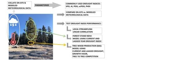
The procedure of this work was as follows. Monthly on-site meteorological data were compiled from different sources and missing data were imputed by rule-based methods. Monthly on-site and modeled (PRISM) meteorological data were compared and modeled data were examined for discrepancies at each site. Five commonly used DIs were parameterized with on-site and PRISM meteorological data. For PDSI-based DIs requiring unknown pedological values, both suggested default values were tested (152 mm and 100 mm). For each site and DI, sources of meteorological data were compared using linear correlation coefficients. We tested the relative performance of DIs parameterized with on-site and modeled meteorology using streamflow (linear correlation), and modeled forest stand NDVI and tree basal area increment (BAI) with current- and lagged-year DI. For predicting BAI, current and lagged DIs were placed within the context of tree vigor and competition metrics using a random effects model. The role of DI’s in predicting BAI was evaluated using the fitted models.
2.3. Collating Meteological Data
Meteorological data were extracted from existing records of daily precipitation, and minimum and maximum air temperature extracted from October 1933 to September 2020 for HM and MF and from October 1939 to September 2020 for SC. The data were obtained from the National Oceanic Atmospheric Administration National Center for Environmental Information Database (NOAA NCEI, [46]), Sequoia National Park archives (obtained from E. Meyer, Research Division, Sequoia-Kings Canyon National Parks), the Western Regional Climate Center (WRCC, [47]), and the National Atmospheric Deposition Program (NADP, [48]). The meteorological data (monthly precipitation sum, average mean air temperature), sources, rule-based methods for accommodating missing data, and metadata have been published [49]. Calculations of potential evapotranspiration (PET, [50]) and parameterizations of the five drought indices (see next section) at the three sites are also contained in posted data. Data were drawn from three meteorological stations: just west of Sunset Rock in Giant Forest, Sequoia National Park (36.5595, −118.7762; 1926 m), 2.03 km W of HM site in a similar topographic position, and 5.76 km SSW of MF site; Lodgepole Village (36.6025, −118.7293, 2043 m), 0.5 km E of the midpoint of the MF site; and Grant Grove Village, Kings Canyon National Park (36.338, −188.9582; 2010 m), 5.5 km WNW of SC.
The following 4 km2 pixels were used to extract modeled meteorological data (PRISM, [14]) for HM (36.5961, −118.7435, 2136 m), MF (36.6203, −118.7488, 2376 m), and SC (36.6673, −118.8325, 2109 m). The mean and range in elevation for each pixel was 2136 m for HM (1775–2650 m); 2109 m for MF (2075–2750 m); and 2275 m for SC (2500–2850 m). PRISM meteorological data was summarized as for the on-site data in [49]. The 800 m pixel data was not available for these sites.
2.4. Parameterization of Drought Indices
All DIs were parameterized with on-site and PRISM meteorological data and reported on an annual (“12”) and hydrologic year (“h,” 10/1 prior yr to 9/30 reported yr) basis, hence “SPEI12h.” All five of the DIs evaluated required calculation of PET. We used the Thornthwaite [50] equation here because it requires only temperature and latitude. The Penman-Monteith calculation is preferred in more moist environments [51,52]. For each of the three sites, the two parameterizations of DIs were tested through the strength of the correlation coefficient. The five DIs were similarly tested among themselves using on-site and then PRISM parameterization.
SPEI was parameterized with summed monthly precipitation, averaged monthly mean air temperature, and location on Earth (latitude as a constraint on radiant energy driving evaporation) to calculate potential evapotranspiration (PET). PET was subtracted from precipitation to quantify deficits and expressed as a distribution-based computation for the convenience of all positive numbers when modeling (log)BAI. Aridity Index (AI) used the same data to calculate the ratio between summed precipitation and mean air temperature [20].
PDSI was developed to quantify drought intensities for crop production and thus considered not only gain and loss of water, but also moisture stored in the soil [21], which SPEI and AI do not. PHDI is a modified version of PDSI and accounts for both development of and recovery from drought [53], with the primary modification of assessing drought termination. PHDI captures the impact of long-term droughts on hydrological balance. While the end of drought is marked by the ratio of PET to precipitation exceeding 0% for PDSI, this ratio is set to 100% in PHDI. scPDSI is another variant of PDSI introduced to improve consistency across regions [22]. For PDSI and derivatives (scPDSI, PHDI; [21,22]), we calculated a monthly drought measurement, the Palmer Z index, which was then summed annually. Because soil available water content (AWC) was not available for our sites, we used the two recommended default values for each PDSI and its derivations, 100 mm and 152 mm. The R package ‘scPDSI’ was used for these calculations [54].
2.5. Independent Tests of DI Effectiveness
2.5.1. Streamflow
The relative performance of current- or prior-year DIs was assessed with the strength of the correlation coefficient, parameterized with on-site or PRISM meteorological data, with a 7 yr hydrologic record (2014 through 2020) of the second-order portion of the Marble Fork Kaweah River. This was the only gauged river immediately associated with our sites, located 0.5 km upstream from the midpoint of the MF site. Streamflow data was recorded every 5 min, extracted from the United States Geological Survey (USGS), National Water Information System [55], and summed monthly.
2.5.2. NDVI
Normalized Difference Vegetation Index (NDVI) is a measure of vegetation response to environmental and meteorological conditions, (NIR−RED)/(NIR + RED), where NIR is near-infrared wavelengths and RED is visible red wavelengths. NDVI was extracted from 18 February 2000 to 29 September 2020 from the NASA Moderate Resolution Imaging Spectroradiometer (MODIS aboard Terra and Aqua satellites). The MOD13Q1 product was corrected for atmospheric and illumination effects and was produced using 16 d composite periods. NDVI values during snowy and cloudy conditions were removed, and the response was smoothed using the cloud computing platform Google Earth Engine [56]. For each site, the maximum number of 250 m × 250 m MODIS pixels (HM, n = 3; MFm, 5; MFx, 3; SC, 5) contained within the polygon of the site were extracted and averaged for the two sample dates in August reflecting the maximum effect of drought on vegetation or summed over the growing season at each site. The growing season length was defined by start-of-season mean air temperature >7 °C to end-of-season mean air temperature <0 °C, resulting in site-specific and sub-site (MFm and MFx) annual values (temperature choices influenced by [57,58,59]. Similar to the approach taken for streamflow, the relative performance of current or prior year DIs was assessed with the fitted linear model R2, parameterized with on-site and PRISM meteorological data, with mean August, or summed NDVI over the growing season.
2.5.3. BAI
Based on a previous analysis of a closely related species (Pinus ponderosa Dougl. ex Laws) also evaluated in dry pine-dominated woodlands to forests, an approach to modeling annual BAI was developed [60] testing current yr and up to 3 yrs prior, and 2 through 4 yr running averages of the DI chosen, as well as a number of crown vigor attributes (see below), insect and disease incidence, and tree-to-tree competition metrics. In the current analysis, we retested current, lagged, and running averages of DIs and biological co-variates for significant explanatories that explained the greatest proportion of the variance in predicting BAI of Jeffrey pine. HM trees were last cored in 2006, and a number of trees had heart rot or resinous centers, so a shorter evaluation period was available (1980–2005). Trees at HM were analyzed separately from the other sites (1980–2005). We modeled BAI of 15 trees at HM using a 25 yr BAI record. MF (MFm, MFx) and SC trees were last cored in 2017 and the BAI chronology was evaluated from 1955 to 2016. We modeled BAI of MFm (n = 17), MFx (n = 16), and SC (n = 20) using a 61 yr BAI record. Because SPEI and AI are highly correlated, and the PDSI variants are highly correlated, we chose only SPEI12h and PDSI12h152 for this analysis. Significance of SPEI or PDSI metrics and the proportion of variance explained in the full model were used to evaluate the two DIs parameterized with on-site and PRISM parameterizations.
Ring width in a cross section of a tree bole is a precise measurement, from which BAI was calculated [61]. Cores were taken within 10 cm of diameter at breast height (DBH, 1.37 m) above the average soil surface to tree center in early to late October, avoiding irregular bark or bole imperfections. Cores were mounted on blocks and sanded to 400 grit. Annual ring widths (early + late wood) were measured to 0.001 mm (Velmex, Inc., Bloomfield, NY, USA) using program J2x, Voor Tech Consulting (2008) and checked for missing rings [62] based on cross-correlation with a regional chronology (Merschel, unpubl. data). Dating accuracy was evaluated using the software program COFECHA (version 6.06P; [63,64]. Potential dating errors identified were visually checked, re-dated, re-measured, or re-collected as necessary. For cores that did not intersect the pith, we estimated the number of rings to the pith geometrically [65] for not more than 4 yrs. BAI for tree i was calculated from radial growth expressed on bole area in the year t minus bole area in year t − 1:
where rt is bole radius at time t.
Tree vigor can affect the capacity of the tree to respond to the environment. ‘RANK’ is a qualitative metric, comprised of several qualitative and quantitative measures (visual assessment of needle color, length, and retention (number of needle ages; retention within a needle age class), branchlet length and diameter), and tree crown structure described and developed for ponderosa pine [38] and applied to Jeffrey pine previously in MFm and MFx [66]. DBH/tree age, here referred to as ‘bole vigor:’ [barkless tree diameter in 1980]/[tree age in 1980 at DBH], a point-in-time measure, roughly a mid-point of this analysis. Competitive zone density (CZD) is a measure of the tree-to-tree competition of each target tree. In each of the four aspects (NE, SE, SW, and NW) to 20 m around the target tree, the DBH of the nearest conspecific tree (>10 cm DBH) divided by the distance from target to neighbor, center to center was measured, and the four measures (DBH/distance) were averaged [40]. This metric was superior to all others tested (variable radius plots; resilience capacity; trees per ha; basal area per ha; and number of trees per cluster [60]) in assessing individual tree response to conspecific competition in its immediate neighborhood.
3. Results
3.1. On-Site vs. PRISM Meteorology
The correlation coefficient between on-site and PRISM precipitation and temperature was 0.98–0.99, respectively, for all three sites. The comparisons are given for MF in Figure 2, and those for HM and SC given in Appendix A and Appendix B. Although monthly PRISM precipitation and temperature data appeared to be well matched to on-site data, seasonal discrepancies were apparent. PRISM temperature data was higher than on-site measurements early in the hydrologic year (November to January) and lower from April to June. An extreme cold event was not predicted by PRISM. There was greater than a 6 °C discrepancy between modeled and on-site temperature during the third week of December 1992 and the first and second weeks of January 1993, which decreased these monthly averages of mean daily air temperature [67].
The discrepancy between on-site and PRISM precipitation was greatest during the period of greatest precipitation, December through April (Figure 2c), when 80% of the annual precipitation is received. Extreme precipitation events (1/1969, 1/1980, 2/1986, and 1/2017) were well outside of the 5% error, and PRISM averaged total annual precipitation for HM, MF, and SC was greater (113 cm, 119 cm, and 115 cm, respectively) than that of on-site data (110 cm, 114 cm, and 106 cm, respectively).
3.2. On-Site vs. PRISM Parameterization of Drought Indices
All DIs generally tracked known high and low precipitation years (MF: Figure 3, HM, SC: Appendix C and Appendix D). Linear correlation coefficients between on-site vs. PRISM meteorological parameterizations of DIs were very high for those evaluated, ranging from 0.87 to 0.99 (Table 1). Although PET and precipitation are components of the DIs investigated, SPEI12h and AI12h were dependent on precipitation to a greater extent than PDSI and its derivatives. SPEI12h had the highest correlation coefficients, and scPDSI had the lowest with 100 mm AWC was slightly lower than that at 152 mm. PDSI and derivatives require additional calculations above those needed for SPEI and AI. We suggest that scPDSI may have the lowest correlation coefficient because it is the most modified from the underlying meteorology (precipitation and temperature) and may be less suited to the hydrology of these sites. Despite strong correlations between the two parameterizations of DIs, PRISM parameterizations reflected the November through June temporal discordance in precipitation (Figure 3). The findings for precipitation at MF also held for HM and SC (Appendix C and Appendix D).
3.3. Correlation among Drought Indices
Linear correlation coefficients between paired DIs within a parameterization (on-site or PRISM) are summarized in Table 2. The correlation coefficients were high and ranged from 0.7 to nearly 1.0. SPEI12h, and AI12h had high correlation coefficients in both on-site and PRISM parameterizations (0.98). Each of the Palmer indices had small differences in correlation coefficients when comparing the two AWC default values. The correlation coefficients were higher between PDSI derivatives at the same AWC level (PDSI152, scPDSI152) and between DIs parameterized with PRISM meteorology, except for PHDI12h where the highest coefficient was obtained with the 100 mm AWC default value (0.989).
3.4. Drought Index Performance Relative to Short-Term Streamflow
The relative performance of the DIs was tested using the strength of the correlation coefficients between current year SPEI at MF and current year streamflow of the Marble Fork Kaweah River over a 7 yr period. SPEI12h and AI2h had the highest correlation coefficients (R > 0.98), using on-site parameterization (Table 3). PDSI and derivatives performed better with PRISM than on-site meteorology perhaps because of a similar spatial scale. Among the PDSI derivatives, PDSI12h performed the best, with slightly improved correlation coefficients using the default AWC of 152 mm. Temporally lagged streamflow (1 yr) was not significantly correlated with precipitation (R = 0.30).
3.5. Drought Index Performance Predicting Site NDVI
Using a model to predict NDVI, the relative performance of the DIs was tested, parameterized with either on-site or PRISM meteorology. A given DI is denoted by Dt with the specified parameterization in year t. We compared the mean August NDVI at HM, SC, and the sub-site MFx against the reference site, MFm. Letting Ys,t be the average August NDVI at site s in year t, we fit the linear model:
Here, centered at zero as independent and identically distributed (i.i.d), Gaussian error terms. is the 0–1 indicator that the observation was at site S. Each DI was standardized (each variable was centered with unit standard deviation) which permitted comparison of coefficients across indices. We also standardized the year variable. Figure 4 shows the data together with the predicted average August NDVI as a function of SPEI, holding all other variables in Equation (2) at their mean values 0.
The estimates and t-tests of the coefficients in Equation (2), fit with DIs parameterized with both on-site and PRISM meteorology, are shown in Table 4. The significance of the DI coefficients varied among the fitted models, and the 1 yr lagged DI was significant for SPEI and AI but not for PDSI152 or PDSI100. Across the DIs and AWC levels tested, and the source of the meteorological data, the model could not differentiate MFm- or MFx-dominated subsites, the latter with quantified differences in tree physiological drought stress between them [44,45]. Only SPEI and AI with on-site parameterizations differentiated SC from MFm. HM was not statistically distinguished from MFm in any of the models. Nonetheless, the overall fit of the model among the indices is similar. The R2 of the models ranged from 0.22 to 0.32. All models designed to predict NDVI with drought indices were similar to one another and of low predictive effectiveness. There was no predictive capacity of the DIs and site-specific, average August, or summed growing season NDVI.
3.6. Drought Index Performance Predicting Site BAI
3.6.1. Predicting BAI at HM
To accommodate one tree with no measurable ring width in one year, 0.01 was added to enable a non-zero log transformation of BAI (log(BAI)) shown in Figure 5. Most HM trees were linearly increasing in BAI early in the chronology shown. Four trees had a different growth pattern from the others, with a peak between 1994 and 1997, suggesting reliance on a water source different from the others at the site. Of the four trees, two were growing out of a rock outcrop and two were in a swale, in deep soil. Adjacent trees in these two settings did not have the same growth pattern. Current year and temporally lagged DI were included in the model and were denoted by Dt, D(t−1), D(t−2), D(t−3) in (3) below. Through a preliminary and exploratory leave-one-out multiple regression, we identified additional factors that modified tree response to the DIs: RANK (with variable R, and the coefficient βR), DBH/AGE (H, βH), and CZD (C, βC). Temporal change in BAI that was not attributable to the above variables was incorporated in a linear term, YEAR. This variable was scaled to avoid computational issues. A tree random effect was also included to model tree to tree variability. Our model for tree i in year t was:
where B0,i and B1,i are i.i.d. centered Gaussian variables. Thus, there was a per-tree random effect accounting for between-tree variability of size and its growth trend. We fit a linear mixed model to the data at HM using SPEI then PDSI, in onsite and PRISM parameterizations. There was no difference in overall fit between the two indices with the same parameterization, and within a DI, the two parameterizations; the marginal R2’s were the same: 0.24.
To assess the role of DI in the model, we compared the full model (3) to one omitting the 4 terms consisting of the DI and its time lags:
The likelihood ratio test comparing Equation (4) to Equation (3) for the two DIs and two parameterizations suggested that there was insufficient evidence to reject the model omitting the DI variables (Table 5). Moreover, the reduced model omitting all DI variables had smaller AIC and BIC in all cases, suggesting the DI variables did not enhance predictions in Equation (4) using only tree attributes. Removing the four trees with different patterns of growth did not change the statistics appreciably, nor our interpretation. Perhaps because different trees may have been relying on different water sources, including the pixel-based meteorological parameterization (PRISM) created a more effective model.
Finally, we evaluated model performance using just DI and temporal lags to predict BAI. We fit the following simple mixed linear model:
The marginal R2 for this model (Equation (5)) suggested little difference between indices (SPEI and PDSI on-site, marginal R2 = 0.03, 0.05, respectively; and SPEI and PDSI PRISM, marginal R2 = 0.04 for both) and demonstrated that the indices alone were inadequate for predicting BAI at HM.
3.6.2. Predicting BAI at MF and SC:
On average, MFm trees had slightly higher BAI (log(BAI)) than MFx; MFx and SC BAI were similar (Figure 6). For many trees at SC, BAI appeared to be independent of known years of limited precipitation. The following years had <80% of long-term average precipitation: 1959–1961, 1964, 1966, 1968, 1970–1972, 1976–1977, 1981, 1987–1992, 1994, 1999, 2004, 2007, and 2012–2015. At SC, two trees had markedly different BAI growth patterns, one within the annual flood plain of Stoney Creek, and the other on a convex, dry slope. When these trees were removed from the model, there was little change in significance or in our interpretation of the model. The response of log(BAI + 0.01) graphed against SPEI12h or PDSI12h was similar (Figure 6).
In the model below, we concurrently predicted BAI of MF and SC, including a factor for site and MF subsites. Let j(i) denote the site of tree i. The model for tree i at time t was:
The terms IA are dummy variables with the value of 1 or 0 corresponding to whether or not condition A was met. The smoothing terms sMFx(t), sMFm(t), and sSC(t) are functions of (t), and B0,i and B1,i are tree-dependent, centered, random Gaussian terms. Each DI was standardized to have mean 0 and unit standard deviation, enabling comparison of coefficients between indices.
Fitted models with site-specific parameterization for each DI are presented in Table 6. Current and 1 yr lagged DI were significant predictors for the on-site parameterizations, although the effect size was very low. Plots of the predicted log(BAI) as a function of SPEI and PDSI, fixing all other variables to their mean values are presented in Figure 7. Over the dynamic range of SPEI and PDSI, predicted log(BAI) did not increase substantially. For example, considering the PDSI at SC (Figure 7, lower right), the expected log (BAI) increased from a minimum of ~2.75 to a maximum of ~2.9 while holding all other variables at their mean values. Tree-to-tree competition was significant for both DIs and parameterizations. Due to the variation among trees, differences among sites and subsites were not significant. All models had similar fits; the marginal R2 for both DIs and parameterizations had the same value: 0.62. Thus, both SPEI and PDSI, parameterized with either on-site or PRISM meteorology performed similarly, and moderately well in predicting BAI at MF and SC. Leaving out ‘bole vigor’ from the otherwise full model reduced the predictive capacity of the model (marginal R2 = 0.23).
To assess the effectiveness of SPEI and PDSI152 alone in predicting BAI with on-site or PRISM parameterization without additional biological covariates, we fit an additional model:
This model exhibited poor performance, with the marginal R2 low (0.14) for both DIs and parameterizations. For the on-site parameterization of SPEI, the estimate of the standard deviation of the random effect (B0,i) was 0.73. This was large relative to the residual error, which had an estimated standard deviation of 0.50. Other indices and parameterizations had similar estimated standard deviations.
4. Discussion
Two types of DIs were evaluated, one based on meteorological and physics-based inputs (SPEI and AI), and the other on meteorological-, physics-, and pedogenic-based inputs (PDSI and derivatives scPDSI and PHDI) in mid-elevation, complex terrain. Relatively few comparisons have been made between on-site and modeled meteorology in these landscapes. While on-site and PRISM monthly mean temperature and summed precipitation were highly correlated, periodic discrepancies in temperature were identified at our sites on the western slope of the Sierra Nevada. PRISM mean temperature was higher than that observed from November to January, and lower for April, May, and June. Higher temperatures in the winter increase ET but would have a low impact on vegetation. Lower temperatures in late spring would decrease calculated DIs and underestimate the level of drought severity when it occurs. In another study across a mid- to high elevation basin on the eastern slope of the Sierra Nevada [16], PRISM maximum temperatures were lower relative to on-site values in early spring (March, April), and mid-summer (July, August). Of interest is that there was an overlap but not an identical match of underestimated monthly temperature between the western (this study) and eastern slopes [16] of the Sierra Nevada, and that the impact of the temperature discrepency would be greater in the latter study as water deficits increase through the summer. During the period of highest precipitation, from November to March, the estimated error variance of PRISM precipitation was high in our study. Extremes, both higher and lower than received, in on-site precipitation exceeded 5% of that estimated by PRISM. Overall, the annual precipitation estimated by PRISM was 3% to 8% greater than received across the three sites. The temperature and precipitation discrepancies of PRISM relative to on-site meteorology both contribute to an underestimation of DI severity during the growing season.
An extreme cold event was not predicted by PRISM (>5 °C discrepancy between modeled and on-site temperature) in December 1992 and January 1993 [67]. Extremely low temperatures on the western slope of the Sierra Nevada are rare but can occur with strong equatorial warming and broadening and deepening of the now permanent year-round lobe of the “winter” arctic jet stream. In December 1992, ‘frigid’ arctic air was reported as far south as southern California, as were exceptionally low minimum temperatures for the first and second weeks of January 1993 [67]. One of the effects of variability in the winter jet stream is that aberrant storm tracks are driven further south along the Pacific coastline [68]. The arctic air mass could have come in over the top of the lower elevation marine air, moving the cold air further up the mountain, as the adjacent, lower elevation Central Valley just east of Visalia had typical daily minimum air temperatures during those events around 0 °C (PRISM daily data for 36.3815, −119.0839, 132 m; explanation suggested by R. Neilson, pers. comm.). An approach to better predicting extreme atmospheric conditions has been proposed [69].
The Marble Fork Kaweah River record was short but included years of low precipitation (<60% of the long-term average) and two of the highest precipitation years of the 90 yr record (>150% of average). Current year DIs were significantly correlated to streamflow. The physics-based DIs, SPEI, and AI, had the highest correlation coefficients (>0.98). PDSI and derived indices had moderate correlation coefficients (0.72 to 0.87), with default AWC values of 152 mm performing better than 100 mm. Prior year DI, regardless of parameterization or type, was not correlated to current year streamflow perhaps because of the short distance between the headwaters and the measurement location, reducing residence and response time [70]. In this environment with highly pulsed precipitation (90% of the annual precipitation is received between November and April) and unknown residence time, forecasts of annual streamflow can be expected to be elusive, although advances in seasonal forecasting have been made [71].
We developed a simple model using current and 1 yr lagged DIs to test their performance in predicting NDVI in the three sites. NDVI is commonly used as a proxy for vegetation productivity, a sensitive indicator of hydrologic drought [72], and an indicator of vegetative degradation from other sources of disturbance [73,74]. NDVI may be particularly applicable to sites dominated by a single species, as investigated here. MODIS-derived NDVI was available for 20 yrs and, except for the 1977 drought year, contained the lowest and all but the highest precipitation year (1969) in the 86 yr precipitation record constructed [49]. In our study, current and lagged year SPEI and PDSI152 were significant explanatories (p ≤ 0.01) of site NDVI, but the linear models had low R2, whether NDVI was represented as a monthly average during period of greatest drawn-down of site water availability (August), or as an integration of site-specific, summed growing season NDVI. All indices and parameterizations performed similarly in tests of predicting NDVI (e.g., low R2). Precipitation five months prior to the growing season (January, coinciding with the period of highest Sierra Nevada precipitation) was significantly correlated with NDVI (also MODIS-derived) [75]. The authors suggested that a long growing season and greater carbon gain in the prior year could have also influenced gross net primary production. In another study, NDVI of individual tree crowns from a fixed-wing platform was one of a number of significant metrics in differentiating low vigor from ‘not low’ vigor crowns in a closely related pine [76]. However, the standard deviation of crown NDVI explained more of the variation than mean crown NDVI (1st vs. 7th most important variable; Random Forest; [76]).
Jeffrey pine in mesic (MFm) and xeric microsites (MFx) could not be differentiated with MODIS-derived NDVI. Morphological crown response to drought (~30% loss of needles mid-crown in the 2007 drought; Grulke, unpubl. data at MF), physiological drought stress [44], elevated foliar oxidative stress [66], and as detected with thermal aerial imagery in 2013 ([45]) clearly differentiated trees in the two subsites at MF. NDVI has been successfully used to validate the use of DIs in vastly different ecosystems (agricultural [77]; chaparral, [78]; forest [79]; and the African continent [80], but in the Californian mixed conifer zone with discontinuous woodlands and forest cover, neither mean August NDVI nor site-specific NDVI summed over the growing season could be used as a validation metric for DI parameterization (however, see [77]).
We then evaluated the role of DIs and the source of their parameterizations in predicting Jeffrey pine BAI. The HM site had a shorter tree ring chronology than MF and SC and was analyzed separately. At HM, none of the five DIs, with either parameterization, at either of the AWC default values, were significant explanatories of BAI. The HM site was downslope (<0.5 km) from Crescent Meadow, which may have acted as a reservoir to buffer annual precipitation inputs, or lack thereof. It is possible that the 1987–1992 drought may not have been long or extreme enough, nor was the single drought year 2002 extreme enough, to reduce the putative supply from the meadow that might have been reflected in BAI. Proximity (distance) to a meadow accounted for 8% of the total variability in canopy water content (using Random Forest, [81]) of giant sequoia (Sequoiadendron giganteum Lind. & Buch.), a species that occurs adjacent to the HM site. In the same area, the underlying geology, and proximity to a stream were significant predictors of crown water content of both giant sequoia and Jeffrey pine in 2015 and 2016 [82]. However, based on isotopic analysis [83], several deciduous desert tree species did not appear to utilize water from an adjacent stream. The trees sampled and presented here were all alive in 2019, 14 yrs after end of the tree ring record analyzed at this site. Patterns of tree BAI at HM were variable, but not more variable than at the other two sites. BAI of four HM trees had a different growth pattern suggesting reliance on a different water source than others in the stand.
A more complex model was developed for MF and SC to predict BAI from current and temporally lagged DIs (SPEI and PDSI152) and biological co-variates (tree crown vigor, bole growth vigor, and tree-to-tree competition). The co-variates tested for Jeffrey pine were selected from an exhaustive analysis of a closely related species, ponderosa pine [60], and were all re-tested in this analysis of Jeffrey pine. Four of the five explanatories were significant using either DI, and the model R2 was moderate (0.62). The fifth explanatory, tree crown vigor, was not significant with either DI or parameterization source, possibly explaining why although DIs were significantly correlated to NDVI, they explained little of the variation. Temporal lags in precipitation were also found to be significant explanatories in a model forecasting the likelihood of tree mortality due to drought and insects (bark beetle, wood borers) in the Sierra Nevada province [84], as well as for temporally lagged SPEI for pine ring width in another summer-dry forest (for Scots pine, (Pinus sylvestris L.), and black pine (Pinus nigra Arn.), in Spain; [85]). Black pine was sensitive to short term drought, but at higher elevation was less so [86]. Jeffrey pine is known to be more drought tolerant than closely related ponderosa pine [87], and perhaps is less sensitive to short term drought as in stone pine (Pinus cembra L.) in the same study [86]. Despite the possibility of long vs. short term drought sensitivities, within-growing season drought significantly affected ring width (index) in black pine. Wood properties, rather than the ring width analyzed in this study, have also been shown to be more responsive than ring widths to climate signals [88], applicable to non-treeline locations.
The hydrology of mid-elevation sites on the western slope of the Sierra Nevada is complex. Jeffrey pine accesses moisture in shallow soil in the spring, but when near-surface horizons dry out, it likely relies on soil pockets in bedrock interstices, trapped moisture under cobbles and boulders, bedrock itself [42,43], surficial and underground seeps, streams, and rivers (however, see [83]). Uphill meadows may also provide a water supply that buffers the impact of droughts [81], as may be the case at our HM site. Individual trees in the same stand may access different water sources, which may vary with residence time, flow or percolation rates, and as well as a possibly unknowable amount of storage in soils and regolith (Cr) [25]. Adjacent trees did not necessarily have the same pattern of growth. The converse was also true: trees in very different microsites (swales with deep soils vs. trees emerging from exposed, cracked bedrock) exhibited similar patterns of BAI. In the central Sierra Nevada, no relationship between Jeffrey pine basal area and soil thickness (A + C, nor Cr) was found [88]. These observations suggest that trees access different sources of water and or there are temporal lags in tree response to similar sources of water.
Considering the complex hydrology and largely unknown or unknowable pedology of these sites suggests that SPEI or AI would be more appropriate indices. However, for predicting BAI in our sites, there was no detectable difference between SPEI and PDSI152 as they exhibited the same correlation coefficient with BAI. In this study, DIs alone (e.g., no biological co-variates), whether parameterized with on-site or modeled meteorological data, were not effective in predicting BAI (R2 = 0.14), and thus in anticipating tree mortality. Surprisingly, despite the different scales of source meteorological data (microsite, point to landscape, and pixel), there was little to no statistical difference in model performance [89].
The Sierra Nevada and Eastern Nevada Province [84] had very high tree mortality in the 2012–2015 drought, an ‘unprecedented drought’ [90]. Although giant sequoia grows in moist sites with deeper soils [82,91], and Jeffrey (and ponderosa) pine grows in thin soils overlying weathered bedrock [24], not all trees sampled of either species responded to the drought [81]. In giant sequoia, lower canopy water content occurred on the margins of groves, at lower elevations further from streams, or in areas of high stand density [81]. Scots pine was more susceptible to drought-induced decline and mortality on forest edges [92]. In our study, we observed high within-site variability BAI in the investigated sites. Adjacent trees in apparently similar microsites had differing BAI patterns, and trees with similar BAI growth patterns occurred in disparate microsites (streamside, dry convex slope). Similar to giant sequoia, some Jeffrey pine were not responsive to drought and others exhibited increased growth regardless of calculated drought severity (e.g., resilience to drought; [93]). In this study, SPEI and PDSI152 with on-site or modeled meteorological parameterizations, performed similarly (R2 = 0.62, MF/SC combined) in predicting BAI only when biological covariates were included in the model. Point-in-time bole growth rates and tree-to-tree competition were significant covariates. Point-in-time bole growth rate, here barkless DBH as a function of tree age at a mid-point in the analysis, was a significant co-variate. In a much larger analysis, larger trees had a disproportionate competitive advantage in mixed age conifer forests [39], and trees with higher bole growth rates were less likely to respond to drought defined by PDSI. The important role of stand- and tree-level competition in bole growth rates has long been established [94,95], and ‘neighborhood’ competition (CZD) was also a significant co-variate in our model.
Trees may succumb quickly or at length to a physical or biological assault. Manion’s [35] ‘death spiral’ suggests mortality in 5 to 8 yrs with multiple insults in long-lived trees. In south central Oregon, ponderosa pine was found to take 40 yrs to succumb after an inciting drought, based on steadily declining BAI to nil (Grulke and Mershel, unpubl. data). Jeffrey pines died in the same year on the eastern edge of the Transverse Range in 1999, the first year of a multi-year drought (1999–2002) (Grulke, pers. obs.). In that range, 25% to 75% tree mortality occurred in stands with greater than 50% tree cover [96]. In the Sierra Nevada, the ‘background’ tree mortality from 2010 to 2014 was 2.7 million trees annually, preceded by a decade of already lower precipitation and higher temperatures than long term records. The 2013, 2014, and 2015 mortality rates were 29, 62, and 27 million trees, respectively, dropping to 19 million trees in 2018 [6], and still elevated 3 to 6 yrs after prolonged ‘hot’ drought as ground water deficits lag precipitation deficits [36].
We can monitor declining canopy water content [97] and pre-emptively anticipate physiological tree drought stress by gaging within-crown thermal differences [45] or oxidative stress (PRI, xanthophyll cycle [98]), but the analysis presented here suggests that biological co-variates, bole growth vigor and tree-to-tree competition, aid in predicting declining BAI. Only the latter co-variate can be assessed remotely. Continuity of mature tree canopies (e.g., greater cover) may be assessed with LiDAR, which is increasingly monitored and available over forested regions. At the California state-wide level [79], a change metric was successfully identified using NDVI that was associated with increased tree mortality 6 to 19 months later [99]. Crown vigor was correlated to ‘bole vigor’ in an analysis of ponderosa pine [60] but was not a significant variant in our model predicting BAI, whether or not bole vigor was also included. The predictive capacity of our model dropped from moderate to poor when bole vigor was not concurrently considered.
Anticipating the meteorological conditions that will lead to extensive tree die-offs in mid- to upper elevations is needed, as loss of vegetation cover will lead to lower on-site water retention and ‘flashier’ downslope flows. DIs alone do not appear to be particularly effective in predicting tree bole growth, an attribute that declines as trees succumb. Conditions and thresholds have been defined that lead to hydraulic failure in trees [100], but the approach may not be scalable in mid to upper elevation forests that rely on regolithic water in the last third to half of the growing season. Estimating the rate of decline, year over year in NDVI [79,100], oxidative stress [99], and or crown or sub-crown thermal imagery [45] could be used as a harbinger of tree decline and mortality, and perhaps with sufficient lead time, for mitigation. We can anticipate loss of water resources with DIs, but at present we only monitor the degradation of mid elevation, open forest Sierran ecosystems with lower water availability and higher temperatures.
5. Conclusions
An 86 yr meteorological record was constructed for mid-elevation sites in the Sierra Nevada, useful for hydrologists, meteorologists, and biologists in future investigations. Correlations between on-site and modeled environmental data within a single DI were high, suggesting that modeled data, ubiquitously used today, can be reliably and interchangeably utilized in research applications in complex terrain. However, periodic discrepancies were discovered in the monthly mean temperature, and the estimated error variance of monthly summed PRISM precipitation exhibited heterogeneity. A similar study on the eastern slope of the Sierra Nevada also observed discrepancies in monthly temperatures, but for different time periods. Correlations among meteorological- and physics-based drought indices (SPEI and AI) and meteorological-, physics-, and pedologically-based drought indices (PDSI and derivatives) were high, suggesting that a similar outcome could be expected from the use of any one of these indices. Correlations of these indices with local streamflow were high, with the highest correlation provided by SPEI and AI. All current year DIs evaluated in this study were unable to predict NDVI in three sites with variable tree densities across this landscape. Drought indices (SPEI or PDSI) accompanied by biological covariates (bole growth vigor, tree-to-tree competition) were moderately predictive of BAI. Although DIs were significant, their effect sizes were low. DIs alone were poor predictors of BAI. This conclusion is robust without regard to which index or parameterization was used. A threshold of some level of meteorological- and physics-based DI such as SPEI or AI may aid predicting biological responses to multiple years of extreme drought but may not permit time for management to mitigate its effects at scale. Rates of change of remotely-detectable tree drought stress, crown vigor, and stand density (canopy continuity) may be a means of identifying high risk locations as well as providing lead time for management.
Author Contributions
Conceptualization, N.E.G.; methodology, Y.K., N.E.G., A.G.M. and K.A.U.; software, Y.K.; validation, Y.K. and A.G.M.; formal analysis, Y.K.; investigation, Y.K., N.E.G., A.G.M. and K.A.U.; resources, N.E.G.; data curation, Y.K. and N.E.G.; writing—original draft preparation, Y.K.; writing—review and editing, N.E.G., A.G.M. and K.A.U.; visualization, Y.K.; supervision, N.E.G.; project administration, N.E.G.; funding acquisition, N.E.G. All authors have read and agreed to the published version of the manuscript.
Funding
This research was funded by the U.S. Department of Agriculture, Forest Service with internal funds. Y.K. was supported by the Forest Service through an National Science Foundation Mathematical Science Graduate Internship Program, and the Oak ridge Institute for Science and Education. This project was supported in part by DISPRO (PMIS No. 119202), a joint U.S. Environmental Protection Agency and National Park Service funding from 1998 to 2002, and NIFA 2007–35101-18144 from 2007–2009. From 2011–2017, funding was provided by the Western Wildlands Environmental Treats Assessment Center, of the US Department of Agriculture, Forest Service. Andrew Merschel was supported by internal funds, from the USFS Pacific Northwest Research Station for measuring and evaluating tree cores.
Institutional Review Board Statement
Not applicable.
Informed Consent Statement
Not applicable.
Data Availability Statement
Data for this analysis is open source and has been archived: Y.K. and N.E.G. (2022). 80-yr meteorological records and drought indices for Sequoia National Park and Sequoia National Monument, CA. U.S. Department of Agriculture, Fort Collins, CO: Forest Service Research Data Archive. RDS-2022-0029. https://0-doi-org.brum.beds.ac.uk/10.2737/RDS-2022-0029 (accessed on 31 March 2022).
Acknowledgments
In memory of Annie Esperanza, who supported this long-term project and data base in many ways, and in memory to Bill Hogsett, for his support for the project from 1998 to 2001 and related projects 2002–2008 that continued to support this research. Special thanks to Erik Meyer for extra effort in finding archived meteorological data for Giant Forest and Lodgepole. Liz Ballenger cored, evaluated, and helped select trees in this study. Thanks to Mac Goelst and Lisa Balduman who extracted tree cores in 2017 and 2018. All evaluations expressed in this paper are the authors’ and do not necessarily reflect the policies and view of the supporting agencies.
Conflicts of Interest
The authors declare no conflict of interest. The project was funded internally by appropriated federal dollars.
Appendix A. On-Site and PRISM Precipitation and Temperature for the HM Site

Appendix B. On-Site and PRISM Precipitation and Temperature for the SC Site

Appendix C. Comparison of On-Site and PRISM Parameterization of PET and the Five Drought Indices at HM

Appendix D. Comparison of On-Site and PRISM Parameterization of PET and the Five Drought Indices at SC

References
- Szejner, P.; Belmecheri, S.; Babst, F.; Wright, W.E.; Frank, D.C.; Hu, J.; Monson, R.K. Stable isotopes of tree rings reveal seasonal-to-decadal patterns during the emergence of a megadrought in the Southwestern US. Oecologia 2021, 197, 1079–1094. [Google Scholar] [CrossRef] [PubMed]
- Ficklin, D.L.; Maxwell, J.T.; Letsinger, S.L.; Gholizadeh, H. A climatic deconstruction of recent drought trends in the United States. Environ. Res. Lett. 2015, 10, 44009. [Google Scholar] [CrossRef]
- Diffenbaugh, N.S.; Swain, D.L.; Touma, D. Anthropogenic warming has increased drought risk in California. Proc. Natl. Acad. Sci. USA 2015, 112, 3931–3936. [Google Scholar] [CrossRef] [PubMed] [Green Version]
- Griffin, D.; Anchukaitis, K.J. How unusual is the 2012–2014 California drought? Geophys. Res. Lett. 2014, 41, 9017–9023. [Google Scholar] [CrossRef] [Green Version]
- Allen, C.R.; Fontaine, J.J.; Pope, K.L.; Garmestani, A.S. Adaptive management for a turbulent future. J. Environ. Manag. 2011, 92, 1339–1345. [Google Scholar] [CrossRef] [PubMed] [Green Version]
- Aerial Detection Survey. 2019. Available online: https://www.fs.usda.gov/Internet/FSE_DOCUMENTS/fseprd700811.pdf (accessed on 31 March 2022).
- Millar, C.I.; Stephenson, N.L. Temperate forest health in an era of emerging megadisturbance. Science 2015, 349, 823–826. [Google Scholar] [CrossRef]
- Allen, C.D.; Breshears, D.D.; McDowell, N.G. On underestimation of global vulnerability to tree mortality and forest die-off from hotter drought in the Anthropocene. Ecosphere 2015, 6, 1–55. [Google Scholar] [CrossRef]
- Adams, H.D.; Guardiola-Claramonte, M.; Barron-Gafford, G.A.; Villegas, J.C.; Breshears, D.D.; Zou, C.B.; Troch, P.A.; Huxman, T.E. Temperature sensitivity of drought-induced tree mortality portends increased regional die-off under global-change-type drought. Proc. Natl. Acad. Sci. USA 2009, 106, 7063–7066. [Google Scholar] [CrossRef] [Green Version]
- McDowell, N.G.; Williams, A.P.; Xu, C.; Pockman, W.T.; Dickman, L.T.; Sevanto, S.; Pangle, R.E.; Limousin, J.M.; Plaut, J.J.; Mackay, D.S.; et al. Multi-scale predictions of massive conifer mortality due to chronic temperature rise. Nat. Clim. Change 2016, 6, 295–300. [Google Scholar] [CrossRef]
- Timmer, K.; Suarez-Brand, M.; Cohen, J.; Clayburgh, J. State of Sierra Waters: A Sierra Nevada Watersheds Index; Sierra Nevada Alliance: Lake Tahoe: Tahoe City, CA, USA, 2006; Available online: https://sierranevadaalliance.org/wpcontent/uploads/sos.pdf (accessed on 15 May 2022).
- Crausbay, S.; Ramirez, A.R.; Carter, S.L.; Cross, M.S.; Hall, K.R.; Bathke, D.J.; Betancourt, J.L.; Colt, S.; Cravens, A.E.; Dalton, M.S.; et al. Defining ecological drought for the twenty-first century. Bull. Am. Meteor. Soc. 2017, 98, 2543–2550. [Google Scholar] [CrossRef]
- Daly, C.; Neilson, R.P.; Phillips, D.L. A statistical-topographic model for mapping climatological precipitation over mountainous terrain. J. Appl. Meteor. Clim. 1994, 33, 140–158. [Google Scholar] [CrossRef] [Green Version]
- PRISM Climate Data. Parameter-elevation Regressions on Independent Slopes Model (PRISM). 2021. Available online: https://prism.oregonstate.edu (accessed on 28 January 2022).
- Daly, C.; Slater, M.E.; Roberti, J.A.; Laseter, S.H.; Swift, L.W., Jr. High-resolution precipitation mapping in a mountainous watershed: Ground truth for evaluating uncertainty in a national precipitation dataset. Int. J. Clim. 2017, 37 (Suppl. S1), 124–137. [Google Scholar] [CrossRef] [Green Version]
- Strachan, S.; Daly, C. Testing the daily PRISM air temperature model on semiarid mountain slopes. J. Geophys. Res. Atmos. 2017, 122, 5697–5715. [Google Scholar] [CrossRef]
- Daly, C.; Conklin, D.R.; Unsworth, M.H. Local atmospheric decoupling in complex topography alters climate change impacts. Int. J. Clim. 2010, 30, 1857–1864. [Google Scholar] [CrossRef]
- Vicente-Serrano, S.M.; Beguería, S.; López-Moreno, J.I. A multi-scalar drought index sensitive to global warming: The Standardized Precipitation Evapotranspiration Index. J. Clim. 2010, 23, 1696–1718. [Google Scholar] [CrossRef] [Green Version]
- Baltas, E. Spatial distribution of climatic indices in northern Greece. Meteor. Appl. 2007, 14, 69–78. [Google Scholar] [CrossRef]
- Budyko, M.E. Climate and Life; Academic Press: New York, NY, USA, 1974; 508p, ISBN 9780080954530. [Google Scholar]
- Palmer, W.C. Meteorological Drought; Research Paper No. 45; U.S. Department of Commerce, Weather Bureau: Washington, DC, USA, 1965; 58p. Available online: http://www.ncdc.noaa.gov/temp-and-precip/drought/docs/palmer.pdf (accessed on 15 May 2022).
- Wells, N.; Goddard, S.; Hayes, M.J. A Self-Calibrating Palmer Drought Severity Index. J. Clim. 2004, 17, 2335–2351. [Google Scholar] [CrossRef]
- Hubbert, K.R.; Beyers, J.L.; Graham, R.C. Roles of weathered bedrock and soil in seasonal water relations of Pinus Jeffreyi and Arctostaphylos patula. Can. J. For. Res. 2001, 31, 1947–1957. [Google Scholar] [CrossRef]
- Rose, K.; Graham, R.C.; Parker, D. Water source utilization by Pinus jeffreyi and Arctostaphylos patula on thin soils over bedrock. Oecologia 2003, 134, 46–54. [Google Scholar] [CrossRef]
- Grulke, N.E. Physiological responses of ponderosa pine to gradients of environmental stressors. In Oxidant Air Pollution Impacts in the Montane Forests of Southern California: A Case Study of the San Bernardino Mountains; Ecological Studies; Miller, P.R., McBride, J.R., Eds.; Springer: New York, NY, USA, 1999; Volume 134, pp. 126–163. [Google Scholar] [CrossRef]
- Beyaztas, U.; Yaseen, Z.M. Drought interval simulation using functional data analysis. J. Hydrol. 2019, 579, 124141. [Google Scholar] [CrossRef]
- Abatzoglou, J.T.; Barbero, R.; Wolf, J.W.; Holden, Z.A. Tracking interannual streamflow variability with drought indices in the U.S. Pacific Northwest. J. Hydrometeorol. 2014, 15, 1900–1912. [Google Scholar] [CrossRef]
- Quemada, C.; Pérez-Escudero, J.M.; Gonzalo, R.; Ederra, I.; Santesteban, L.G.; Torres, N.; Iriarte, J.C. Remote sensing for plant water content monitoring: A review. Remote Sens. 2021, 13, 2088. [Google Scholar] [CrossRef]
- Berner, L.T.; Law, B.E.; Hudiburg, T.W. Water availability limits tree productivity, carbon stocks, and carbon residence time in mature forests across the western US. Biogeosciences 2017, 14, 365–378. [Google Scholar] [CrossRef] [Green Version]
- Li, Z.; Zhou, T.; Zhao, X.; Huang, K.; Gao, S.; Wu, H.; Luo, H. Assessments of drought impacts on vegetation in China with the optimal time scales of the Climatic Drought Index. Int. J. Environ. Res. Public Health 2015, 12, 7615–7634. [Google Scholar] [CrossRef] [Green Version]
- Vincente-Serrano, S.M.; Gouveia, C.; Camarero, J.J.; Begueria, S.; Sanchez-Lorenzo, A. Response of vegetation to drought time-scales across global land biomes. Proc. Natl. Acad. Sci. USA 2021, 110, 52–57. [Google Scholar] [CrossRef] [Green Version]
- Drew, D.M.; Allen, K.; Downes, G.M.; Evans, R.; Battaglia, M.; Baker, P. Wood properties in a long-lived conifer reveal strong climate signals where ring-width series do not. Tree Physiol. 2012, 33, 37–47. [Google Scholar] [CrossRef] [Green Version]
- Pompa-García, M.; Camarero, J.J.; Colangelo, M.; González-Cásares, M. Inter- and intra-annual links between climate, tree growth and NDVI: Improving the resolution of drought proxies in conifer forests. Int. J. Biometeorol. 2021, 65, 2111–2121. [Google Scholar] [CrossRef]
- Pasho, E.; Alla, A.Q. Climate impacts on radial growth and vegetation activity of two co-existing Mediterranean pine species. Can. J. For. Res. 2015, 45, 1748–1756. [Google Scholar] [CrossRef] [Green Version]
- Manion, P.D. Tree Disease Concept, 2nd ed.; Prentice Hall: Hoboken, NJ, USA, 1981; 399p, ISBN 978013930701037. [Google Scholar]
- Su, L.; Cao, Q.; Xiao, M.; Mocko, D.M.; Barlage, M.; Li, D.; Peters-Lidard, C.D.; Lettenmaier, D.P. Drought variability over the conterminous United States for the past century. J. Hydrometeorol. 2021, 22, 1153–1168. [Google Scholar] [CrossRef]
- Preisler, H.K.; Grulke, N.E.; Heath, Z.; Smith, S.L. Analysis and out-year forecast of beetle, borer, and drought-induced tree mortality in California. For. Ecol. Manag. 2017, 399, 166–178. [Google Scholar] [CrossRef]
- Grulke, N.E.; Bienz, C.; Hrinkevich, K.; Maxfield, J.; Uyeda, K. Quantitative and qualitative approaches to assess effectiveness of forest treatments in improving stand health in dry pine forests. For. Ecol. Manag. 2020, 465, 118085. [Google Scholar] [CrossRef]
- Looney, C.E.; D’Amato, A.W.; Jovan, S. Investigating linkages between the size-growth relationship and drought, nitrogen deposition, and structural complexity in western U.S. Forests. For. Ecol. Manag. 2021, 497, 119494. [Google Scholar] [CrossRef]
- Shaw, R. Tree Vigor Response and Competitive Zone Density in Mature Ponderosa Pine. Master’s Thesis, Oregon State University, Corvallis, OR, USA, 2017; 85p. Available online: https://ir.library.oregonstate.edu/concern/graduate_thesis_or_dissertations/mc87ps84d (accessed on 25 February 2021).
- Barbour, M.G.; Minnich, R.A. Californian upland forests and woodlands. In North American Terrestrial Vegetation; Barbour, M.G., Billings, W.D., Eds.; Cambridge University Press: Cambridge, UK, 1999; pp. 161–202. ISBN 052155027. Available online: http://catdir.loc.gov/catdir/samples/cam031/97029061.pdf (accessed on 15 May 2022).
- Jones, D.P.; Graham, R.C. Water-holding characteristics of weathered granitic rock in chaparral and forest ecosystems. Soil Sci. Soc. Am. J. 1993, 57, 256–261. [Google Scholar] [CrossRef]
- McCormick, E.L.; Dralle, D.N.; Hahm, W.J.; Tune, A.K.; Schmidt, L.M.; Chadwick, K.D.; Rempe, D.M. Widespread woody plant use of water stored in bedrock. Nature 2021, 597, 225–229. [Google Scholar] [CrossRef] [PubMed]
- Grulke, N.E.; Johnson, R.; Esperanza, A.; Jones, D.; Nguyen, T.; Posch, S.; Tausz, M. Canopy transpiration of Jeffrey pine in mesic and xeric microsites: O3 uptake and injury response. Trees 2003, 17, 292–298. [Google Scholar] [CrossRef]
- Grulke, N.E.; Maxfield, J.; Riggan, P.J.; Schrader-Patton, C.S. Pre-emptive detection of mature pine drought stress using multispectral aerial imagery. Remote Sens. 2020, 12, 2338. [Google Scholar] [CrossRef]
- National Oceanic and Atmosphere Administration (NOAA); National Centers for Environmental Information (NCEI). Climate Data Records. Available online: https://www.ncei.noaa.gov/products/climate-data-records (accessed on 31 March 2022).
- Western Regional Climate Center (WRCC). Southwest Climate and Environmental Information Collaborative (SCENIC), Reno, NV, USA, 1933–2020. Available online: https://wrcc.dri.edu/csc/scenic/ (accessed on 22 February 2022).
- National Atmospheric Deposition Program. (NRSP-3) (NADP), NTN SITE: CA75. Available online: https://nadp.slh.wisc.edu/networks/national-trends-network/ (accessed on 25 February 2022).
- Kim, Y.; Grulke, N.E. 80-Yr Meteorological Records and Drought Indices for Sequoia National Park and Sequoia National Monument, CA; Forest Service Research Data Archive, RDS-2022-0029; U.S. Department of Agriculture: Fort Collins, CO, USA, 2022. [Google Scholar] [CrossRef]
- Thornthwaite, C.W. An approach toward a rational classification of climate. Geogr. Rev. 1948, 38, 55–94. [Google Scholar] [CrossRef]
- Stannard, D.I. Comparison of Penman-Monteith, Shuttleworth-Wallace, and Modified Priestley-Taylor Evapotranspiration Models for wildland vegetation in semiarid rangeland. Water Resour. Res. 1993, 29, 1379–1392. [Google Scholar] [CrossRef]
- Allen, R.G.; Pereira, L.S.; Raes, D.; Smith, M. Crop Evapotranspiration—Guidelines for Computing Crop Water Requirements; FAO Irrigation and Drainage Paper 56; Food and Agriculture Organization, United Nations: Rome, Italy, 1998; 15p, Available online: https://appgeodb.nancy.inra.fr/biljou/pdf/Allen_FAO1998.pdf (accessed on 15 May 2022).
- Karl, T.R. The sensitivity of the Palmer Drought Severity Index and Palmer’s Z-Index to their calibration coefficients including potential evapotranspiration. J. Appl. Meteor. Clim. 1986, 25, 77–86. [Google Scholar] [CrossRef] [Green Version]
- Zhong, R.; Chen, X.; Wang, Z.; Lai, C. scPDSI: Calculation of the Conventional and Self-Calibrating Palmer Drought Severity Index. 2018. Available online: https://rdrr.io/cran/scPDSI/ (accessed on 18 May 2022).
- United States Geological Survey (USGS); National Water Information System (NWIS). USGS Water Data for the Nation Help. Available online: https://help.waterdata.usgs.gov (accessed on 25 February 2022).
- Gorelick, N.; Hancher, M.; Dixon, M.; Ilyushchenko, S.; Thau, D.; Moore, R. Google Earth Engine: Planetary-scale geospatial analysis for everyone. Remote Sens. Environ. 2017, 202, 18–27. [Google Scholar] [CrossRef]
- Dougherty, P.M.; Whitehead, D.; Vose, J.M. Environmental Influences on the phenology of pine. Ecol. Bull. 1994, 43, 64–75. Available online: https://0-www-jstor-org.brum.beds.ac.uk/stable/20113132?seq=1#metadata_info_tab_contents (accessed on 15 May 2022).
- Sloan, J.P. Ponderosa and Lodgepole Pine Seedling Bud Burst Varies with Lift Date and Cultural Practices in Idaho Nursery; RN-INT-397; U.S. Department of Agriculture, Forest Service, Intermountain Research Station: Ogden, UT, USA, 1991; 9p, Available online: https://www.worldcat.org/title/ponderosa-and-lodgepole-pine-seedling-bud-burst-varies-with-lift-date-and-cultural-practices-in-idaho-nursery/oclc/679979260&referer=brief_results (accessed on 15 May 2022).
- Andersen, C.P.; Sucoff, E.I.; Dixon, R.K. Effects of root zone temperature on root initiation and elongation in red pine seedlings. Can. J. For. Res. 1986, 16, 696–700. [Google Scholar] [CrossRef]
- Levin, D.A.; Grulke, N.E.; Bienz, C.; Hrinkevich, K.; Merschel, A.; Uyeda, K.A. Forest treatment effects on wood production in ponderosa pine. For. Ecol. Manag. 2022, in press. Available online: https://pages.uoregon.edu/dlevin/PAPERS/sycan.pdf (accessed on 15 May 2022).
- Stokes, M.A.; Smiley, T.L. An Introduction to Tree Ring Dating; University of Arizona Press: Flagstaff, AZ, USA, 1996; 73p, ISBN 9780816516803. [Google Scholar]
- Yamaguchi, D.K. A simple method for cross-dating increment cores from living trees. Can. J. For. Res. 1991, 21, 414–416. [Google Scholar] [CrossRef]
- Grissino-Mayer, H.D. Evaluating crossdating accuracy: A manual and tutorial for the computer program COFECHA. Tree-Ring Res. 2000, 57, 205–221. Available online: https://www.ltrr.arizona.edu/~ellisqm/outgoing/dendroecology2014/readings/Grissino_mayer_COFECHA_2001.pdf (accessed on 15 May 2022).
- Holmes, R.L. Computer-assisted quality control in tree-ring dating and measurement. Tree-Ring Bull. 1983, 43, 69–78. Available online: https://www.ltrr.arizona.edu/~ellisqm/outgoing/dendroecology2014/readings/Holmes_1983.pdf (accessed on 15 May 2022).
- Applequist, M.B. A simple pith locator for use with off-center increment cores. J. For. 1958, 56, 141. Available online: https://0-academic-oup-com.brum.beds.ac.uk/jof/article/56/2/138/4685764?login=true92 (accessed on 15 May 2022).
- Grulke, N.E.; Johnson, R.; Monschein, S.; Nikolova, P.; Tausz, M. Variation in morphological and biochemical O3 injury attributes of mature Jeffrey pine within canopies and between microsites. Tree Physiol. 2003, 23, 923–929. [Google Scholar] [CrossRef] [Green Version]
- University of Minnesota. United States Monthly Climate Summary. December 1992–January 1993. Available online: https://www.google.com/books/edition/Weekly_Climate_Bulletin/YRYs5pcurcoC?hl=en&gbpv=1&dq=%22united+states+monthly+climate+summary+December+1992%22&pg=PA11&printsec=frontcover (accessed on 22 February 2022).
- Athanasiadis, P.J.; Wallace, J.M.; Wettstein, J.J. Patterns of wintertime jet Stream variability and their relation to the storm tracks. J. Atmos. Sci. 2010, 67, 1361–1381. [Google Scholar] [CrossRef]
- Deo, R.C.; Şahin, M. Application of the extreme learning machine algorithm for the prediction of monthly Effective Drought Index in eastern Australia. Atmos. Res. 2015, 153, 512–525. [Google Scholar] [CrossRef] [Green Version]
- Bales, R.C.; Goulden, M.L.; Hunsaker, C.T.; Conklin, M.H.; Hartsough, P.C.; O’Geen, A.T.; Hopmans, J.; Safeeq, M. Mechanisms controlling the impact of multi-year drought on mountain hydrology. Sci. Rep. 2018, 8, 690. [Google Scholar] [CrossRef] [PubMed] [Green Version]
- Pechlivanidis, I.G.; Crochemore, L.; Rosberg, J.; Bosshard, T. What are the key drivers controlling the quality of seasonal streamflow forecasts? Water Resour. Res. 2020, 56, e2019WR026987. [Google Scholar] [CrossRef]
- Yuhas, A.N.; Scuderi, L.A. MODIS-derived NDVI characterisation of drought-induced evergreen die-off in western North America. Geogr. Res. 2009, 47, 34–45. [Google Scholar] [CrossRef]
- Easdale, M.H.; Bruzzone, O.; Mapfumo, P.; Tittonell, P. Phases or regimes? Revisiting NDVI trends as proxies for land degradation. Land Degrad. Dev. 2018, 29, 433–445. [Google Scholar] [CrossRef]
- Hargrove, W.W.; Spruce, J.P.; Gasser, G.E.; Hoffman, F.M. Toward a national early warning system for forest disturbances using remotely sensed canopy phenology. Photogramm. Eng. Remote Sens. 2009, 75, 1150–1156. Available online: https://www.fs.usda.gov/treesearch/pubs/33669 (accessed on 15 May 2022).
- Wong, C.Y.S.; Young, D.J.N.; Latimer, A.M.; Buckley, T.N.; Magney, T.S. Importance of the legacy effect for assessing spatiotemporal correspondence between interannual tree-ring width and remote sensing products in the Sierra Nevada. Remote Sens. Environ. 2021, 265, 112635. [Google Scholar] [CrossRef]
- Schrader-Patton, C.; Grulke, N.E.; Bienz, C. Landscape assessment of ponderosa pine vigor using 4-Band aerial imagery in south central Oregon. Forests 2021, 12, 612. [Google Scholar] [CrossRef]
- Lu, J.; Carbone, G.J.; Gao, P. Mapping the agricultural drought based on the long-term AVHRR NDVI and North American Regional Re-analysis (NARR) in the United States, 1981–2013. Appl. Geogr. 2019, 104, 10–20. [Google Scholar] [CrossRef]
- Uyeda, K.A.; Stow, D.A.; Roberts, D.A.; Riggan, P.J. Combining ground-based measurements and MODIS-based spectral vegetation indices to track biomass accumulation in post-fire chaparral. Int. J. Remote Sens. 2017, 38, 718–741. [Google Scholar] [CrossRef]
- Liu, Y.; Kumar, M.; Katul, G.G.; Porporato, A. Reduced resilience as an early warning signal of forest mortality. Nature Clim. Change 2019, 9, 880–885. Available online: https://0-www-nature-com.brum.beds.ac.uk/articles/s41558-019-0583-9 (accessed on 15 May 2022). [CrossRef]
- Peng, J.; Dadson, S.; Hirpa, F.; Dyer, E.; Lees, T.; Miralles, D.G.; Vicente-Serrano, S.M.; Funk, C. A pan-African high-resolution drought index dataset. Earth Syst. Sci. Data 2020, 12, 753–769. [Google Scholar] [CrossRef] [Green Version]
- Paz-Kagan, T.; Vaughn, N.R.; Martin, R.E.; Brodrick, P.G.; Stephenson, N.L.; Das, A.J.; Nydick, K.R.; Asner, G.P. Landscape-scale variation in canopy water content of giant sequoias during drought. For. Ecol. Manag. 2018, 419–420, 291–304. [Google Scholar] [CrossRef] [Green Version]
- Baeza, A.; Martin, R.E.; Stephenson, N.L.; Das, A.J.; Hardwick, P.; Nydick, K.; Mallory, J.; Slaton, M.; Evans, K.; Asner, G.P. Mapping the vulnerability of giant sequoias after extreme drought in California using remote sensing. Ecol. Appl. 2021, 31, e02395. [Google Scholar] [CrossRef] [PubMed]
- Dawson, T.E.; Ehleringer, J.R. Streamside trees that do not use Stream water. Nature 1991, 350, 335–337. [Google Scholar] [CrossRef]
- Miles, S.R.; Goudey, C.B. (Comps.) Ecological Sub-Regions of California: Section and Subsection Descriptions; R5-EM-TP-005; USDA Forest Service, Technical Publication, Pacific Southwest Region: Vallejo, CA, USA, 1997; 200p. [Google Scholar]
- Martin-Benito, D.; Beeckman, H.; Cañellas, I. Influence of drought on tree rings and tracheid features of Pinus nigra and Pinus sylvestris in a mesic Mediterranean forest. Eur. J. For. Res. 2012, 132, 33–45. [Google Scholar] [CrossRef]
- Bhuyan, U.; Zang, C.; Menzel, A. Different responses of multispecies tree ring growth to various DIs across Europe. Dendrochronologia 2017, 44, 1–8. [Google Scholar] [CrossRef]
- Staszak, J.; Grulke, N.E.; Marrett, M.J.; Prus-Glowacki, W. Isozyme markers associated with O3 tolerance indicate shift in genetic structure of ponderosa and Jeffrey pine in Sequoia National Park, California. Environ. Pollut. 2007, 149, 366–375. [Google Scholar] [CrossRef]
- Meyer, M.D.; North, M.P.; Gray, A.N.; Zald, H.S.J. Influence of soil thickness on stand characteristics in a Sierra Nevada mixed-conifer forest. Plant Soil 2007, 294, 113–123. [Google Scholar] [CrossRef]
- Potter, K.A.; Woods, H.A.; Pincebourde, S. Microclimate challenges in global change biology. Glob. Change Biol. 2013, 10, 2932–2939. [Google Scholar] [CrossRef]
- Robeson, S.M. Revisiting the recent California drought as an extreme value. Geophys. Res. Lett. 2015, 42, 6771–6779. [Google Scholar] [CrossRef]
- Su, Y.; Bales, R.C.; Ma, Q.; Nydick, K.; Ray, R.L.; Li, W.; Guo, Q. Emerging stress and relative resiliency of giant sequoia groves experiencing multiyear dry periods in a warming climate. J. Geophys. Res. Biogeosci. 2017, 122, 3063–3075. [Google Scholar] [CrossRef] [Green Version]
- Buras, A.; Schunk, C.; Zeiträg, C.; Herrmann, C.; Kaiser, L.; Lemme, H.; Straub, C.; Taeger, S.; Gößwein, S.; Klemmt, H.-J.; et al. Are Scots pine forest edges particularly prone to drought-induced mortality? Environ. Res. Lett. 2018, 13, 25001. [Google Scholar] [CrossRef]
- Lloret, F.; Keeling, E.G.; Sala, A. Components of tree resilience: Effects of successive low-growth episodes in old ponderosa pine forests. Oikos 2011, 120, 1909–1920. [Google Scholar] [CrossRef]
- Oliver, C.D.; Larson, B.A. Forest Stand Dynamics. Updated Edition. In Yale School of the Environment 1; John Wiley & Sons: Hoboken, NJ, USA, 1996; Available online: https://elischolar.library.yale.edu/fes_pubs/1/ (accessed on 15 May 2022).
- Biging, G.S.; Dobbertin, M. Evaluation of competition indices in individual tree growth models. For. Sci. 1995, 41, 360–377. [Google Scholar]
- Grulke, N.E.; Paine, T.; Minnich, R.; Chavez, D.; Riggan, P.; Dunn, A. Air pollution increases forest susceptibility to wildfire. In Wildland Fires and Air Pollution; Developments in Environmental Science; Bytnerowicz, A., Arbaugh, M., Riebau, A., Andersen, C., Eds.; Elsevier Publishers: The Hague, The Netherlands, 2009; Volume 8, pp. 365–403. [Google Scholar] [CrossRef]
- Asner, G.P. Progressive forest canopy water loss during the 2012–2015 California drought. Proc. Natl. Acad. Sci. USA 2016, 113, E249–E255. [Google Scholar] [CrossRef] [Green Version]
- Wong, C.Y.S.; Gamon, J.A. Three causes of variation in the photochemical reflectance index (PRI) in evergreen conifers. New Phytol. 2015, 206, 187–195. Available online: https://0-www-jstor-org.brum.beds.ac.uk/stable/newphytologist.206.1.187 (accessed on 15 May 2022). [CrossRef]
- Bell, D.M.; Cohen, W.B.; Reilly, M.; Yang, Z. Visual interpretation and time series modeling of Landsat imagery highlight drought’s role in forest canopy declines. Ecosphere 2018, 9, e02195. [Google Scholar] [CrossRef]
- Anderegg, W.R.L.; Berry, J.A.; Smith, D.D.; Sperry, J.S.; Anderegg, L.D.L.; Field, C.B. The roles of hydraulic and carbon stress in a widespread climate-induced forest die-off. Proc. Natl. Acad. Sci. USA 2012, 109, 233–237. [Google Scholar] [CrossRef] [Green Version]
Figure 1.
Location of study sites (triangles) and meteorological stations (stars) in Sequoia National Park (Marble Fork, MF; Huckleberry Meadow, HM) and Monument (Stoney Creek, SC).
Figure 1.
Location of study sites (triangles) and meteorological stations (stars) in Sequoia National Park (Marble Fork, MF; Huckleberry Meadow, HM) and Monument (Stoney Creek, SC).

Figure 2.
Comparison of on-site vs. PRISM (a) precipitation; (b) mean air temperature; (c,d) and discrepancies between the two at site MF.
Figure 2.
Comparison of on-site vs. PRISM (a) precipitation; (b) mean air temperature; (c,d) and discrepancies between the two at site MF.

Figure 3.
On-site vs. PRISM parameterization of PET and each drought index calculated for the hydrologic year.
Figure 3.
On-site vs. PRISM parameterization of PET and each drought index calculated for the hydrologic year.

Figure 4.
Predicted site average August NDVI for the three sites (MF, HM, and SC) and two subsites (MFmesic and MFxeric).
Figure 4.
Predicted site average August NDVI for the three sites (MF, HM, and SC) and two subsites (MFmesic and MFxeric).

Figure 5.
Log(BAI + 0.01) at HM vs. year for a subset of trees showing different patterns of tree bole growth at the same site.
Figure 5.
Log(BAI + 0.01) at HM vs. year for a subset of trees showing different patterns of tree bole growth at the same site.

Figure 6.
Log(BAI + 0.01) at the two MF subsites and SC showing different responses to SPEI (left) and PDSI152 (right).
Figure 6.
Log(BAI + 0.01) at the two MF subsites and SC showing different responses to SPEI (left) and PDSI152 (right).

Figure 7.
Predicted log(BAI + 0.01) as a function of on-site and PRISM parameterizations of SPEI and PDSI152. Other variables included in the model (Equation (6)) are fixed at their mean values (tree crown vigor, bole growth vigor, and tree competition).
Figure 7.
Predicted log(BAI + 0.01) as a function of on-site and PRISM parameterizations of SPEI and PDSI152. Other variables included in the model (Equation (6)) are fixed at their mean values (tree crown vigor, bole growth vigor, and tree competition).


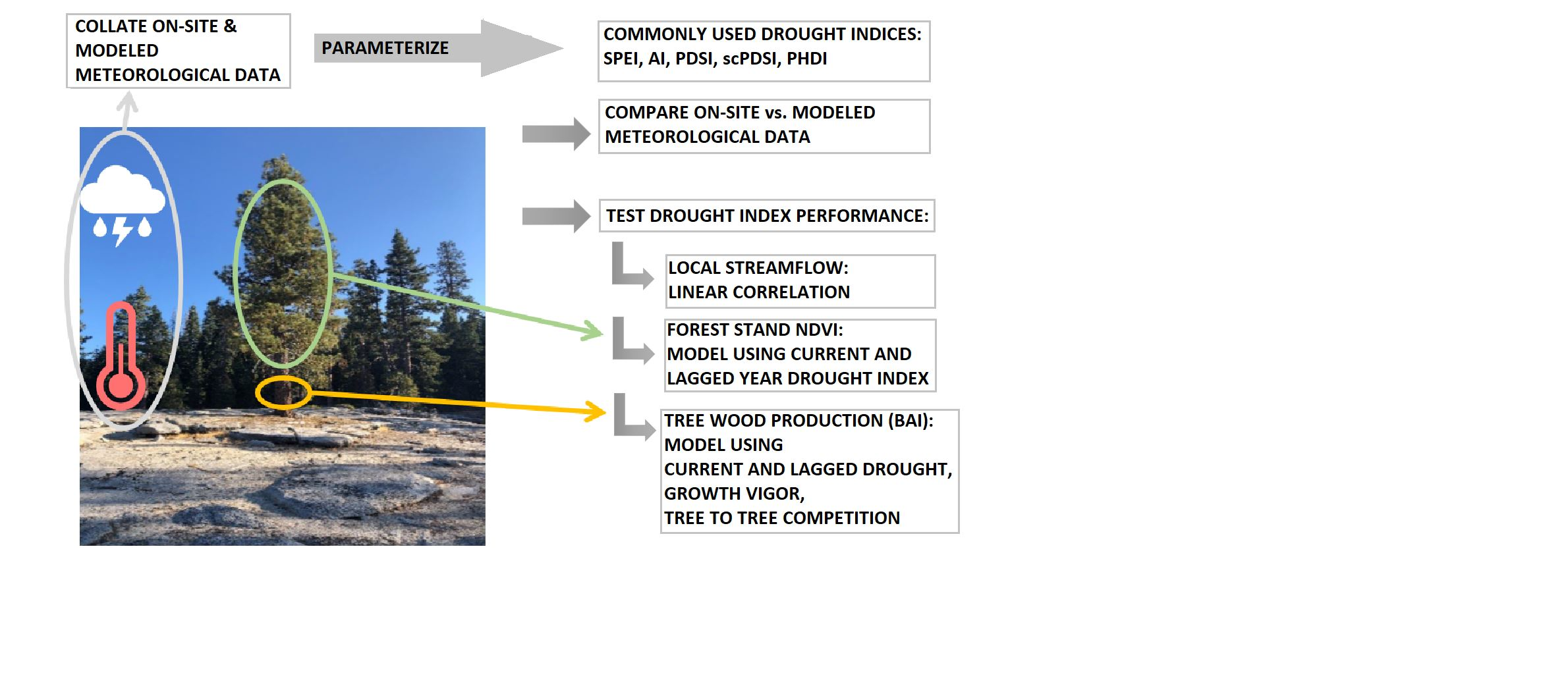
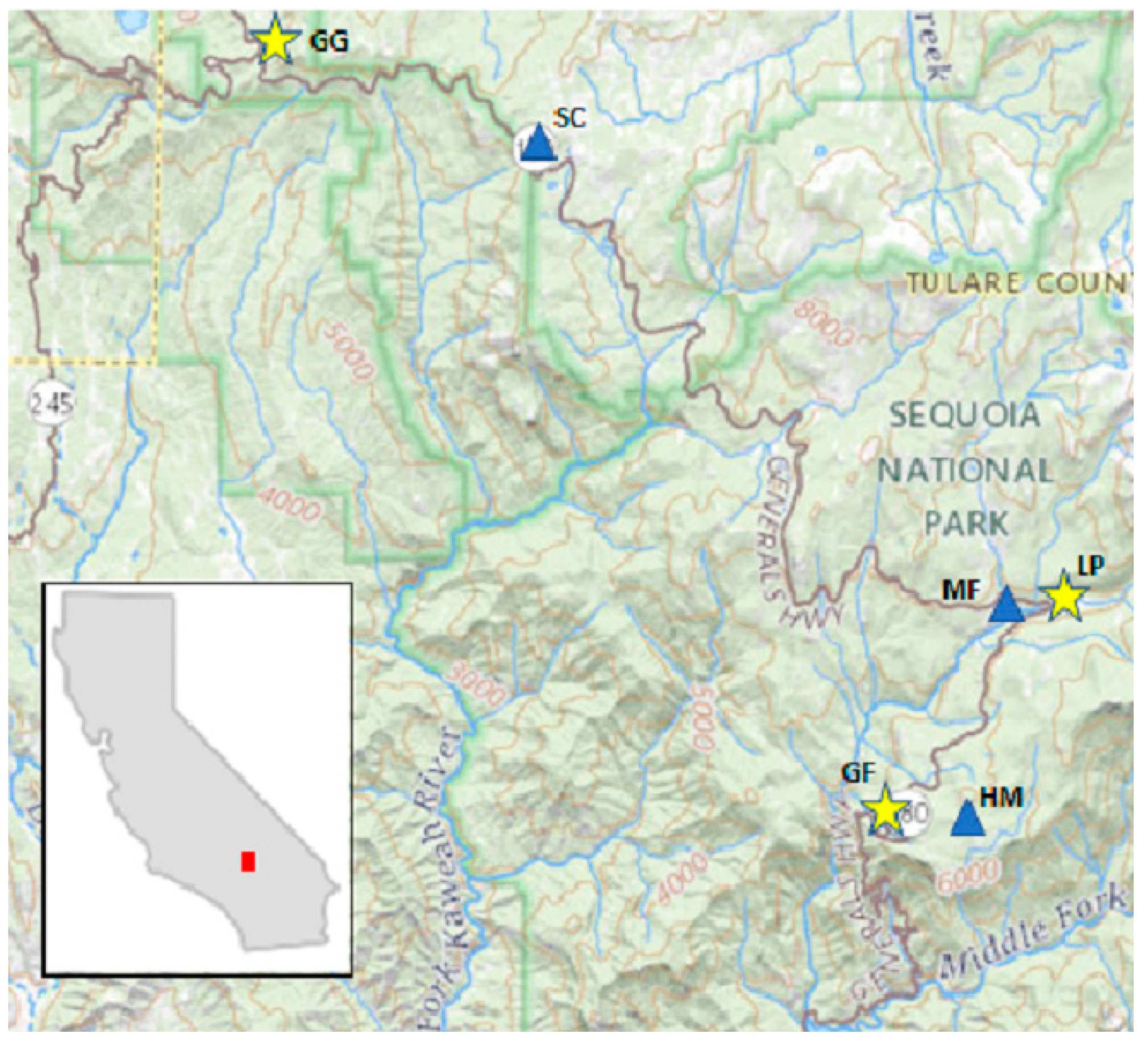
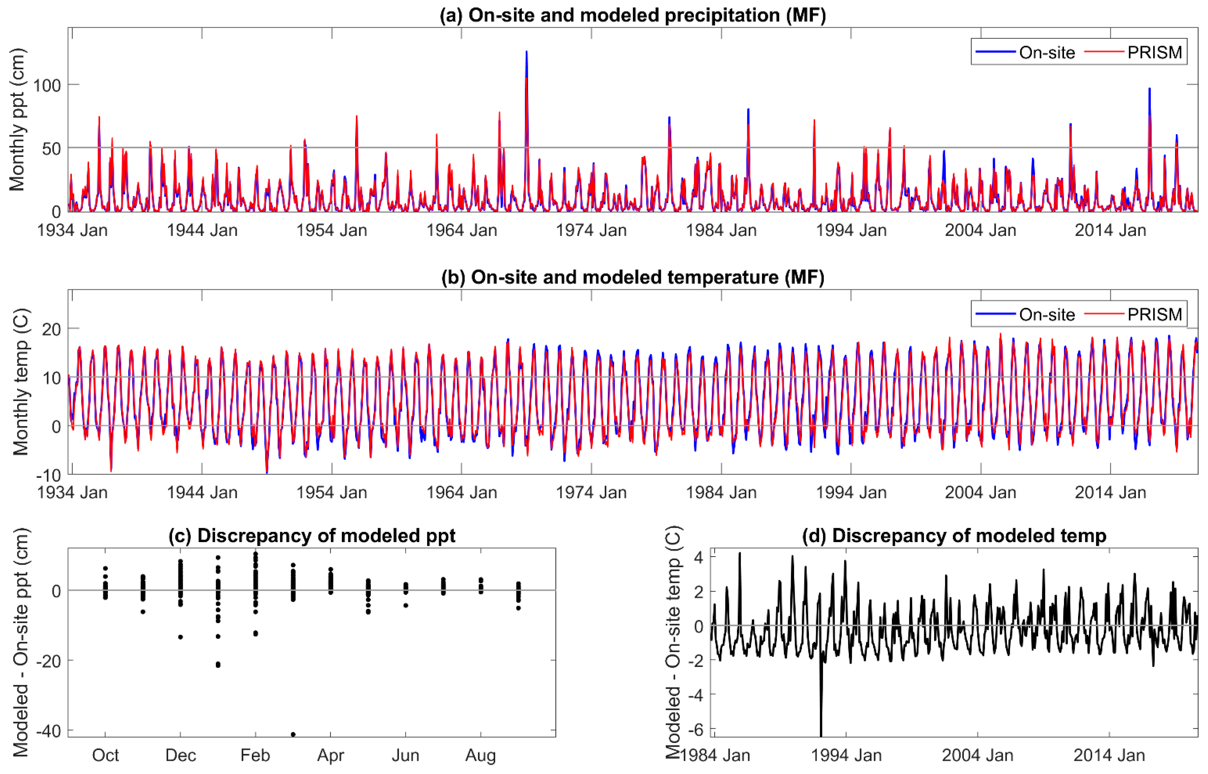
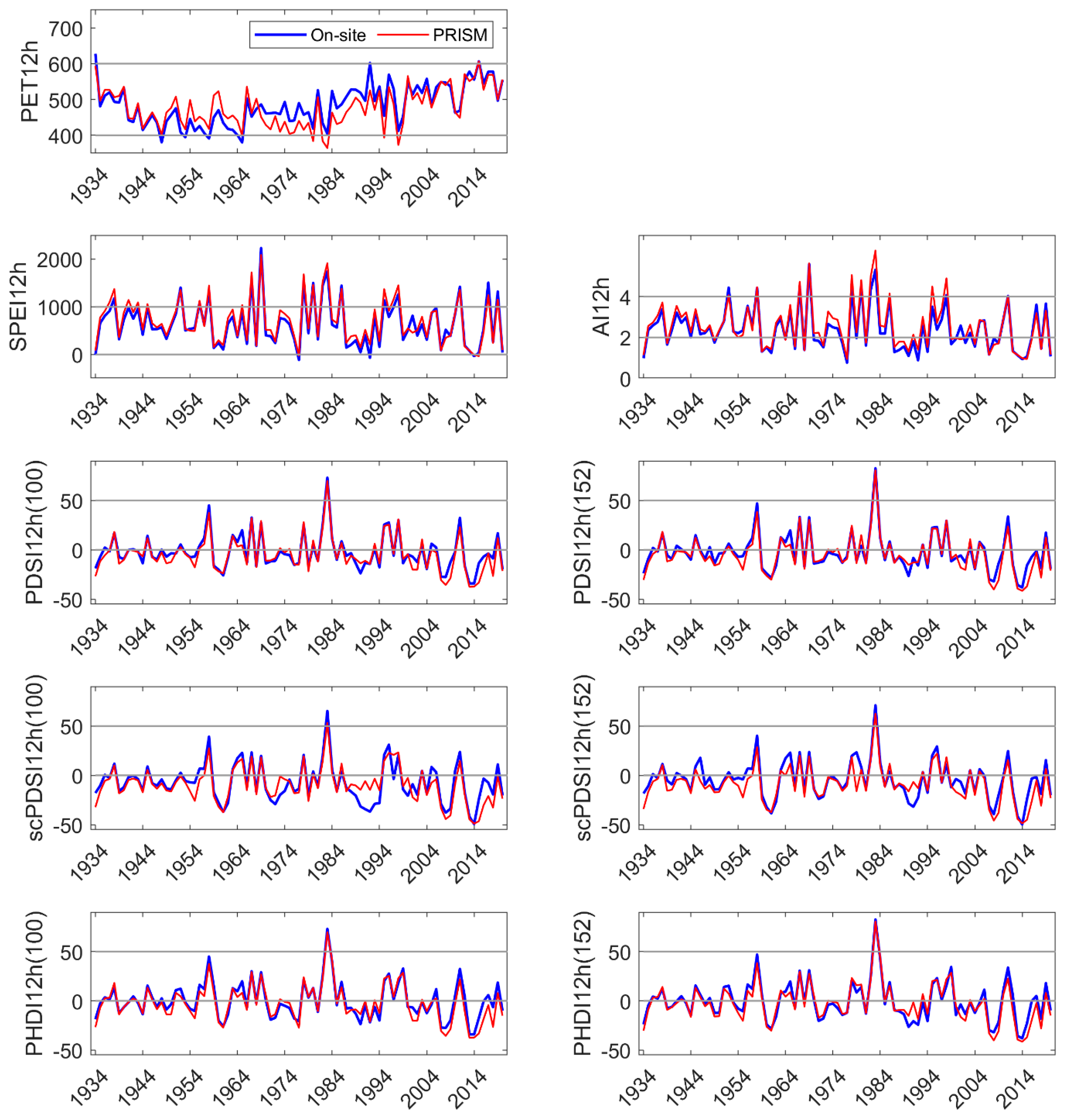
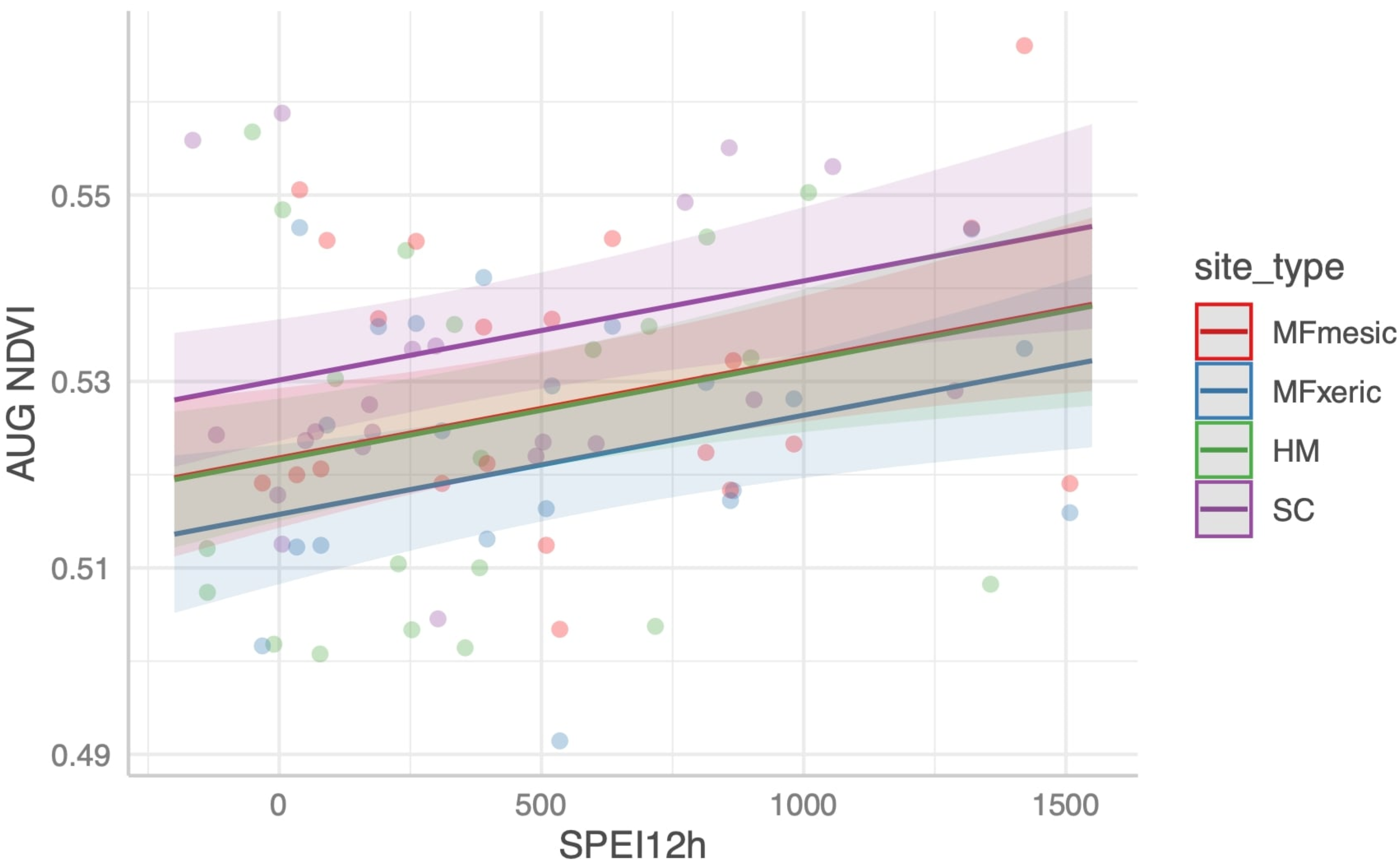
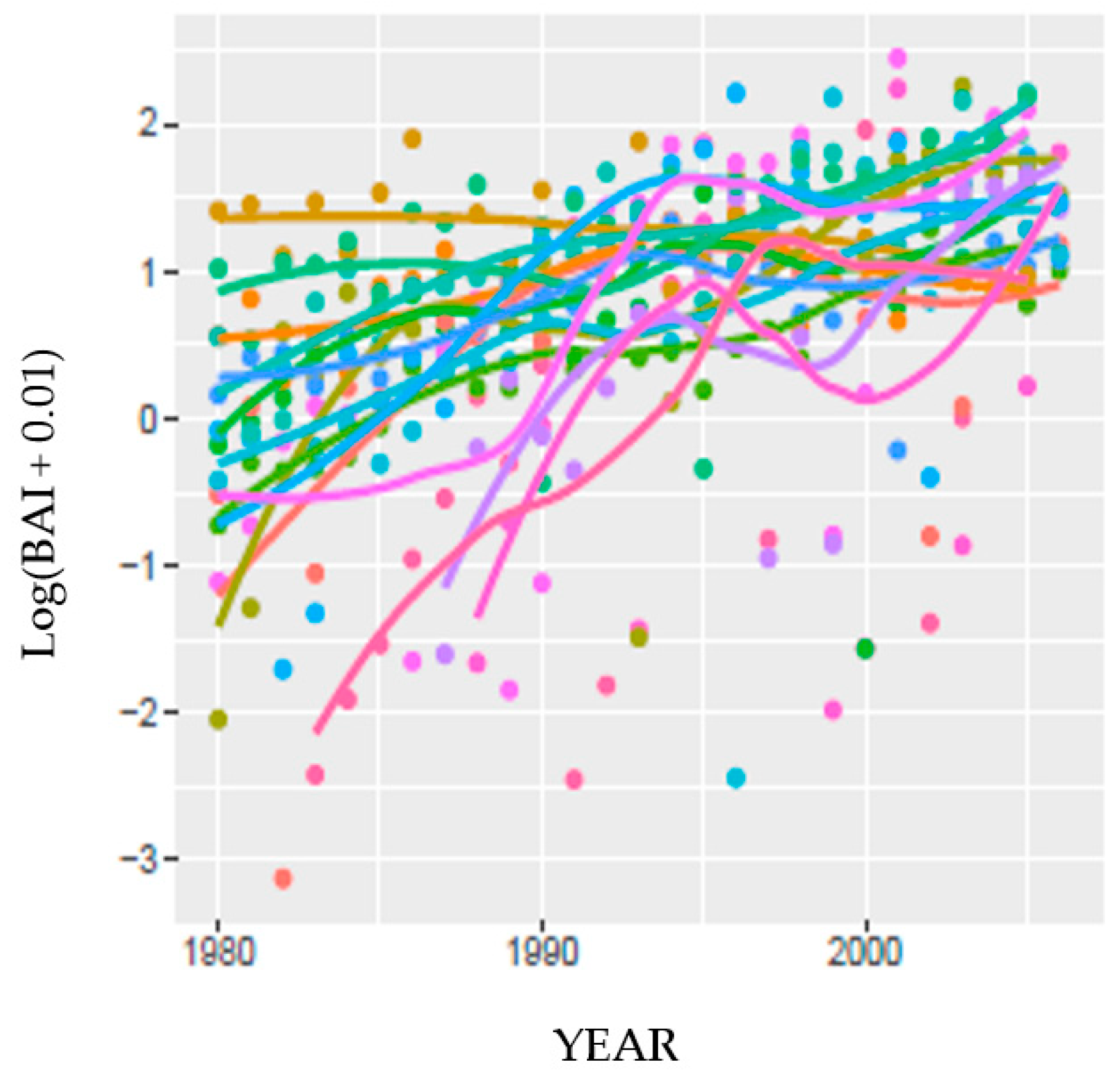
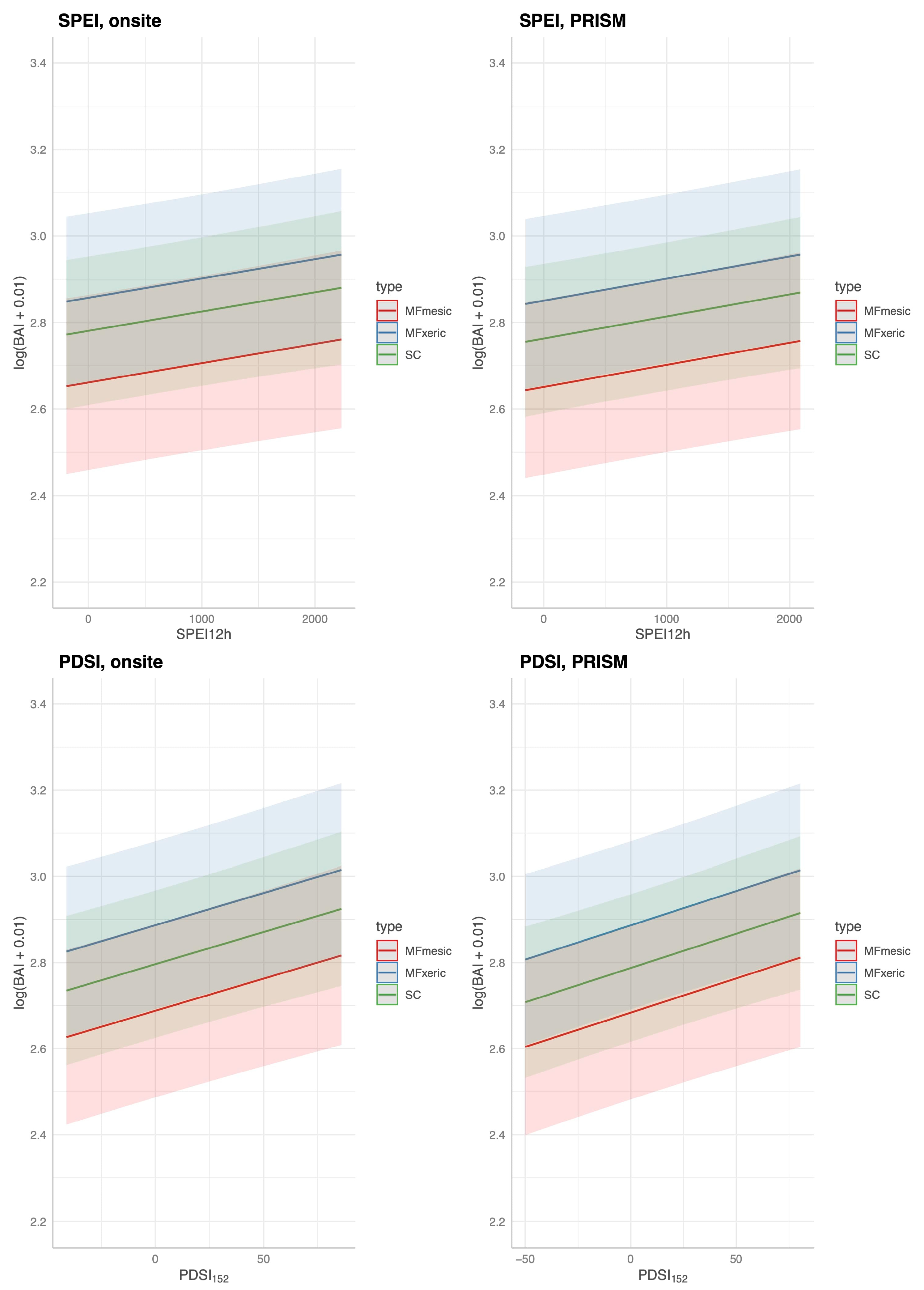
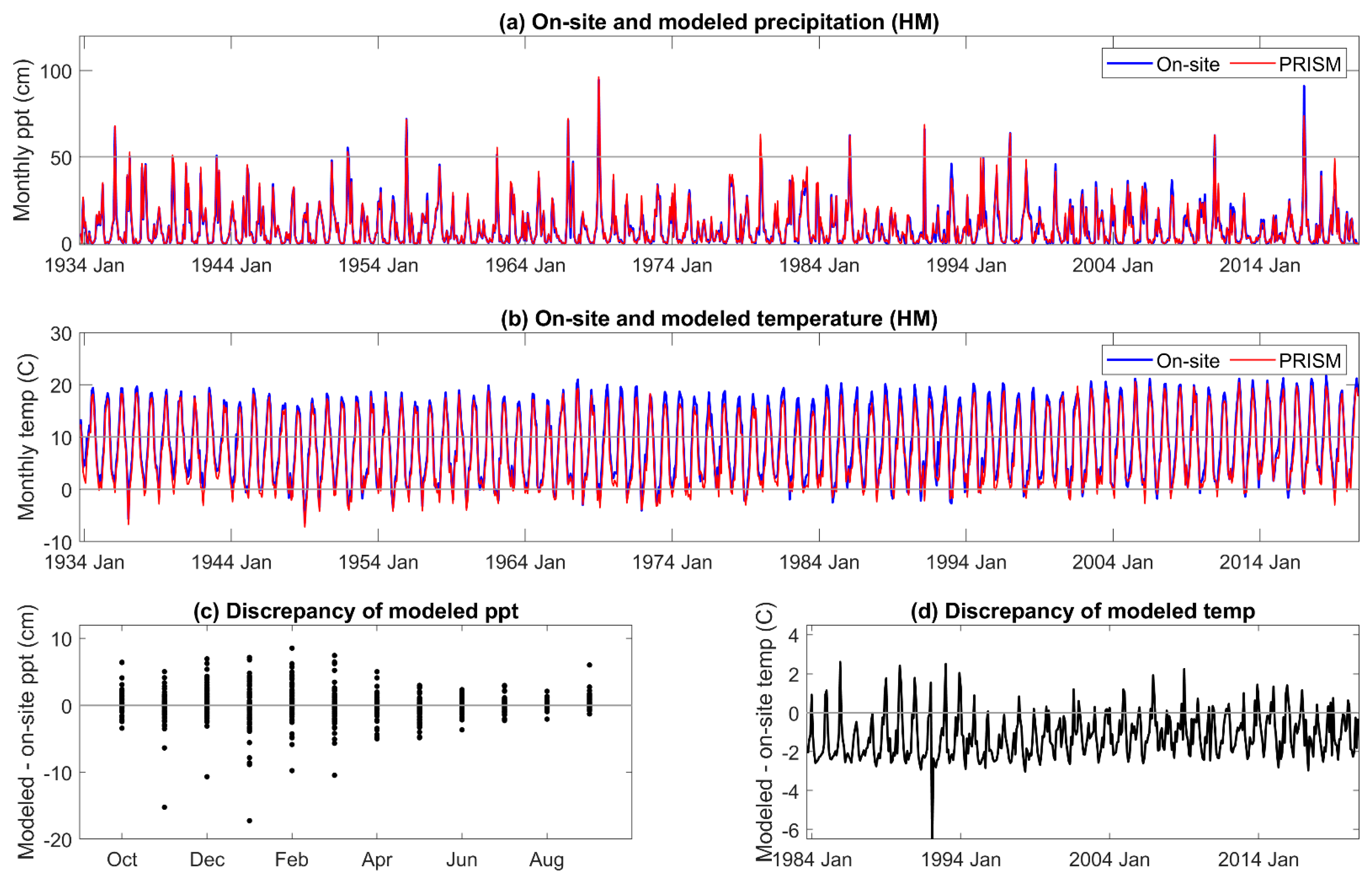
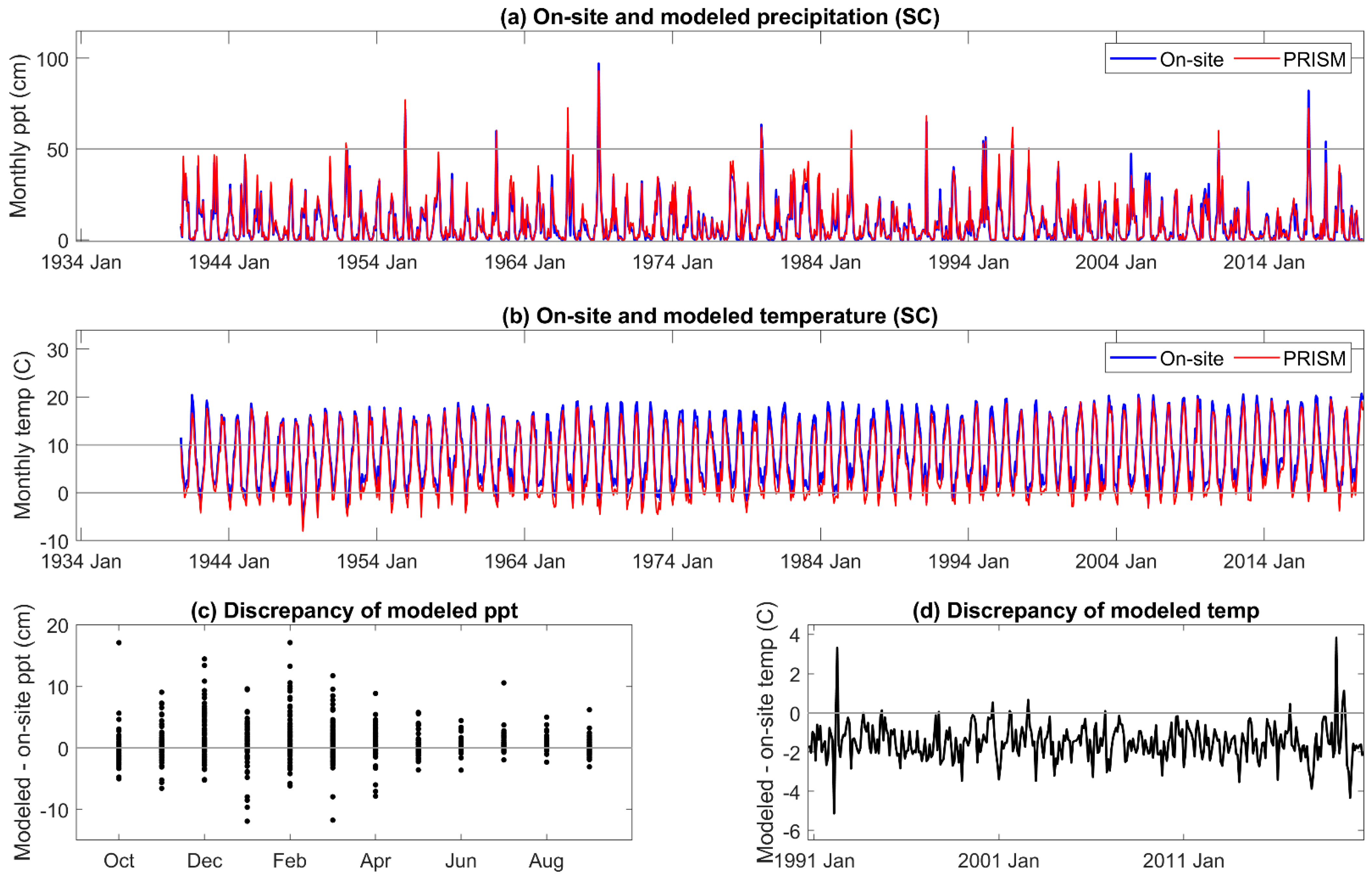
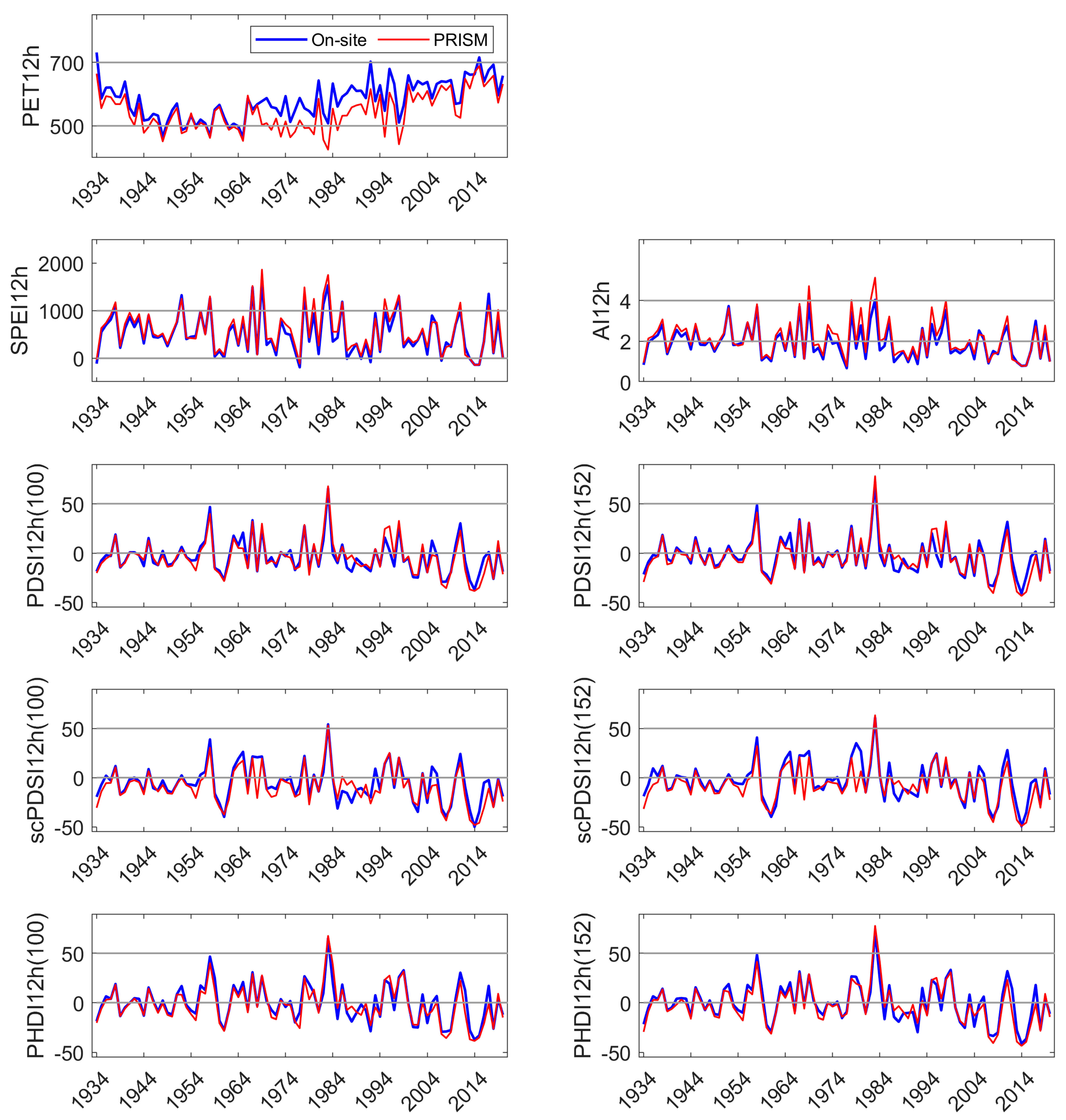
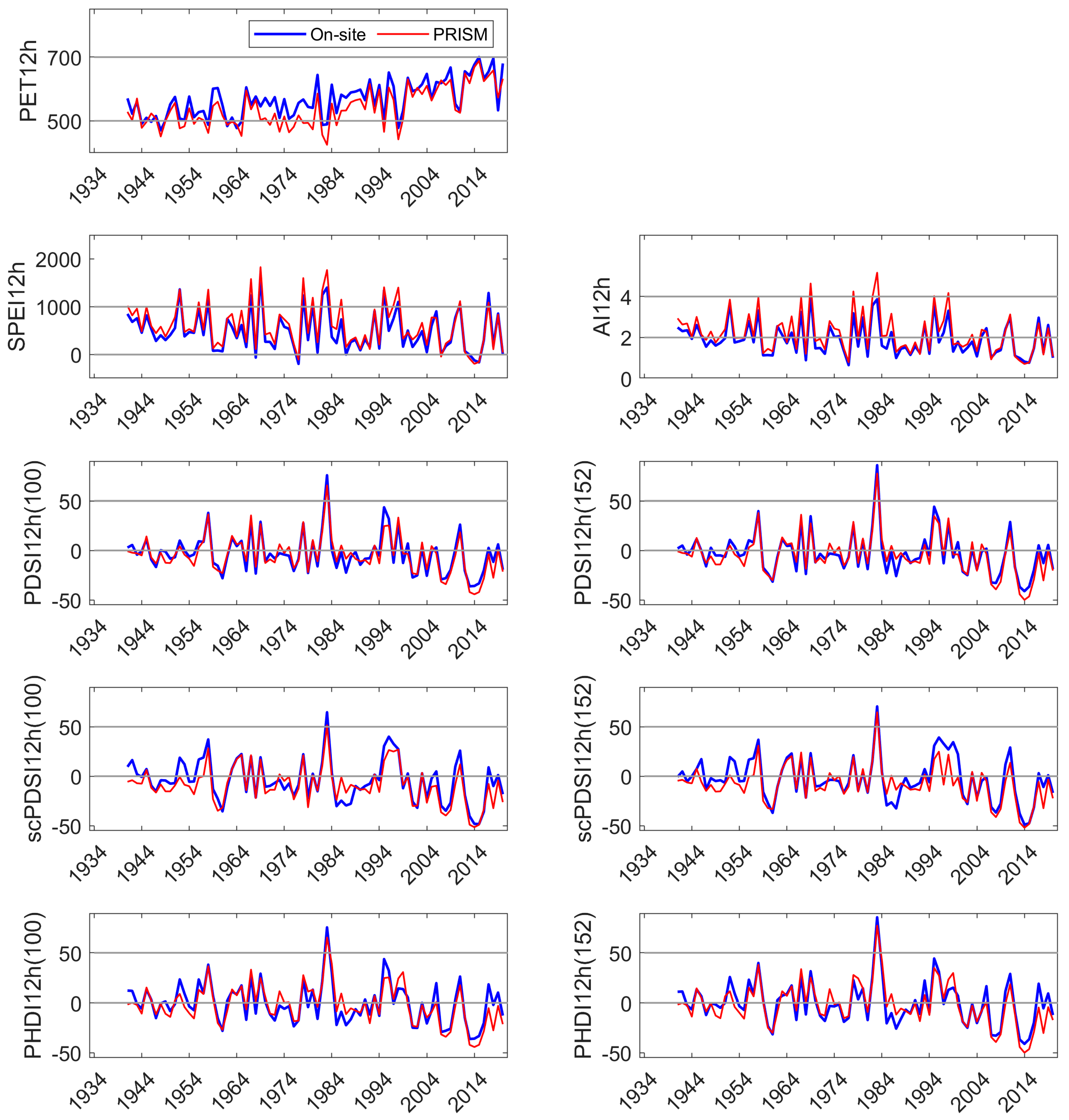
Table 1.
Correlation coefficients between on-site vs. PRISM meteorologically parameterized drought indices at each site (MF, HM, and SC). PET and all drought indices were calculated on an annual basis over the hydrologic year (10/1 through 9/30).
Table 1.
Correlation coefficients between on-site vs. PRISM meteorologically parameterized drought indices at each site (MF, HM, and SC). PET and all drought indices were calculated on an annual basis over the hydrologic year (10/1 through 9/30).
| INDEX | MF | HM | SC |
|---|---|---|---|
| PET12h | 0.99 | 0.99 | 1.00 |
| SPEI12h | 0.98 | 0.98 | 0.97 |
| AI12h | 0.97 | 0.97 | 0.97 |
| PDSI12h152 | 0.96 | 0.95 | 0.95 |
| PDSI12Hh100 | 0.95 | 0.94 | 0.94 |
| scPDSI12h152 | 0.91 | 0.88 | 0.88 |
| scPDSI12h100 | 0.87 | 0.90 | 0.92 |
| PHDI12h152 | 0.95 | 0.95 | 0.91 |
| PHDI12h100 | 0.95 | 0.94 | 0.90 |
Table 2.
Correlation coefficients between drought indices as parameterized by on-site and PRISM (in parentheses).
Table 2.
Correlation coefficients between drought indices as parameterized by on-site and PRISM (in parentheses).
| SPEI12h | AI12h | PDSI12h152 | PDSI12h100 | scPDSI12h152 | scPDSI12h100 | PHDI12h152 | |
|---|---|---|---|---|---|---|---|
| AI12h | 0.98 (0.98) | ||||||
| PDSI12h152 | 0.81 (0.85) | 0.81 (0.85) | |||||
| PDSI12h100 | 0.81 (0.85) | 0.81 (0.86) | 0.99 (0.99) | ||||
| scPDFI12h152 | 0.71 (0.82) | 0.70 (0.82) | 0.90 (0.98) | 0.88 (0.97) | |||
| scPDFI12h100 | 0.72 (0.81) | 0.72 (0.80) | 0.91 (0.95) | 0.91 (0.95) | 0.93 (0.97) | ||
| PHDI12h152 | 0.75 (0.77) | 0.75 (0.77) | 0.90 (0.91) | 0.88 (0.90) | 0.89 (0.91) | 0.88 (0.88) | |
| PHDI12h100 | 0.75 (0.78) | 0.75 (0.78) | 0.89 (0.91) | 0.89 (0.91) | 0.88 (0.90) | 0.88 (0.89) | 0.99 (0.99) |
Table 3.
Correlations between on-site and PRISM-parameterized drought indices and local streamflow.
| SPEI12h | AI12h | PDSI12h152 | PDSI12h100 | scPDSI12h152 | scPDSI12h100 | PHDI12h152 | PHDI12h100 | |
|---|---|---|---|---|---|---|---|---|
| On-site | 1.00 | 0.98 | 0.80 | 0.74 | 0.78 | 0.72 | 0.82 | 0.81 |
| PRISM | 0.99 | 0.98 | 0.88 | 0.88 | 0.87 | 0.74 | 0.85 | 0.84 |
Table 4.
Fitted models predicting NDVI from on-site or PRISM parameterized drought indices.
| Estimate | S. E. | t Value | Pr(>|t|) | Estimate | S. E. | t Value | Pr(>|t|) | ||
|---|---|---|---|---|---|---|---|---|---|
| SPEI/ON-SITE | PDSI152/ON-SITE | ||||||||
| (Intercept) | 0.5268 | 0.0031 | 168.83 | 0.00 | (Intercept) | 0.5296 | 0.0033 | 160.66 | 0.00 |
| site_typeMFxeric | −0.0061 | 0.0043 | −1.41 | 0.16 | site_typeMFxeric | −0.0061 | 0.0046 | −1.30 | 0.20 |
| site_typeHM | −0.0002 | 0.0045 | −0.04 | 0.96 | site_typeHM | −0.0060 | 0.0047 | −1.28 | 0.20 |
| site_typeSC | 0.0084 | 0.0046 | 1.82 | 0.07 | site_typeSC | 0.0029 | 0.0047 | 0.62 | 0.53 |
| scale(SPEI12h_nolag) | 0.0047 | 0.0017 | 2.81 | 0.01 | scale(SPEI12h_nolag) | 0.0058 | 0.0019 | 3.00 | 0.00 |
| scale(SPEI12h_lag1) | 0.0064 | 0.0016 | 4.03 | 0.00 | scale(SPEI12h_lag1) | 0.0022 | 0.0018 | 1.24 | 0.22 |
| scale(SPEI12h_lag2) | 0.0028 | 0.0016 | 1.81 | 0.08 | scale(SPEI12h_lag2) | 0.0011 | 0.0018 | 0.06 | 0.55 |
| scale(SPEI12h_lag3) | 0.0042 | 0.0017 | 2.46 | 0.02 | scale(SPEI12h_lag3) | 0.0037 | 0.0020 | 1.84 | 0.07 |
| scale(YEAR) | 0.0034 | 0.0016 | 2.19 | 0.03 | scale(YEAR) | 0.0044 | 0.0018 | 2.43 | 0.02 |
| SPEI/PRISM | PDSI152/PRISM | ||||||||
| (Intercept) | 0.5282 | 0.0031 | 169.33 | 0.00 | (Intercept) | 0.5300 | 0.0032 | 163.34 | 0.00 |
| site_typeMFxeric | −0.0061 | 0.0044 | −1.39 | 0.17 | site_typeMFxeric | −0.0061 | 0.0046 | −1.32 | 0.19 |
| site_typeHM | −0.0021 | 0.0045 | −0.46 | 0.64 | site_typeHM | −0.0068 | 0.0046 | −1.48 | 0.14 |
| site_typeSC | 0.0045 | 0.0044 | 1.01 | 0.32 | site_typeSC | 0.0021 | 0.0046 | 0.45 | 0.65 |
| scale(SPEI12h_nolag) | 0.0047 | 0.0017 | 2.78 | 0.01 | scale(SPEI12h_nolag) | 0.0059 | 0.0019 | 3.06 | 0.00 |
| scale(SPEI12h_lag1) | 0.0061 | 0.0016 | 3.85 | 0.00 | scale(SPEI12h_lag1) | 0.0027 | 0.0018 | 1.55 | 0.13 |
| scale(SPEI12h_lag2) | 0.0014 | 0.0016 | 0.87 | 0.39 | scale(SPEI12h_lag2) | 0.0000 | 0.0019 | −0.02 | 0.98 |
| scale(SPEI12h_lag3) | 0.0035 | 0.0018 | 1.98 | 0.05 | scale(SPEI12h_lag3) | 0.0036 | 0.0021 | 1.70 | 0.09 |
| scale(YEAR) | 0.0047 | 0.0017 | 2.74 | 0.01 | scale(YEAR) | 0.0058 | 0.0021 | 2.80 | 0.01 |
| AI/ON-SITE | PDSI100/ON-SITE | ||||||||
| (Intercept) | 0.5257 | 0.0032 | 163.13 | 0.00 | (Intercept) | 0.5292 | 0.0033 | 162.55 | 0.00 |
| site_typeMFxeric | −0.0061 | 0.0043 | −1.40 | 0.17 | site_typeMFxeric | −0.0061 | 0.0046 | −1.32 | 0.19 |
| site_typeHM | 0.0024 | 0.0048 | 0.50 | 0.62 | site_typeHM | −0.0054 | 0.0046 | −1.17 | 0.25 |
| site_typeSC | 0.0101 | 0.0048 | 2.10 | 0.04 | site_typeSC | 0.0040 | 0.0047 | 0.85 | 0.40 |
| scale(SPEI12h_nolag) | 0.0050 | 0.0017 | 2.93 | 0.00 | scale(SPEI12h_nolag) | 0.0061 | 0.0019 | 3.24 | 0.00 |
| scale(SPEI12h_lag1) | 0.0067 | 0.0016 | 4.09 | 0.00 | scale(SPEI12h_lag1) | 0.0026 | 0.0017 | 1.55 | 0.13 |
| scale(SPEI12h_lag2) | 0.0022 | 0.0016 | 1.37 | 0.18 | scale(SPEI12h_lag2) | 0.0012 | 0.0018 | 0.69 | 0.49 |
| scale(SPEI12h_lag3) | 0.0034 | 0.0017 | 1.98 | 0.15 | scale(SPEI12h_lag3) | 0.0039 | 0.0019 | 2.05 | 0.04 |
| scale(YEAR) | 0.0036 | 0.0016 | 2.20 | 0.03 | scale(YEAR) | 0.0043 | 0.0018 | 2.44 | 0.02 |
| AI/PRISM | PDSI100/PRISM | ||||||||
| (Intercept) | 0.5276 | 0.0032 | 165.45 | 0.00 | (Intercept) | 0.5301 | 0.0032 | 164.10 | 0.00 |
| site_typeMFxeric | −0.0061 | 0.0044 | −1.38 | 0.17 | site_typeMFxeric | −0.0061 | 0.0046 | −1.33 | 0.19 |
| site_typeHM | −0.0006 | 0.0047 | −0.14 | 0.89 | site_typeHM | −0.0070 | 0.0046 | −1.53 | 0.13 |
| site_typeSC | 0.0053 | 0.0046 | 1.17 | 0.25 | site_typeSC | 0.0017 | 0.0046 | 0.36 | 0.72 |
| scale(SPEI12h_nolag) | 0.0048 | 0.0017 | 2.83 | 0.01 | scale(SPEI12h_nolag) | 0.0058 | 0.0018 | 3.12 | 0.00 |
| scale(SPEI12h_lag1) | 0.0061 | 0.0016 | 3.77 | 0.00 | scale(SPEI12h_lag1) | 0.0030 | 0.0017 | 1.77 | 0.08 |
| scale(SPEI12h_lag2) | 0.0006 | 0.0017 | 0.37 | 0.71 | scale(SPEI12h_lag2) | −0.0005 | 0.0019 | −0.25 | 0.81 |
| scale(SPEI12h_lag3) | 0.0028 | 0.0018 | 1.55 | 0.13 | scale(SPEI12h_lag3) | 0.0032 | 0.0020 | 1.61 | 0.11 |
| scale(YEAR) | 0.0045 | 0.0018 | 2.53 | 0.01 | scale(YEAR) | 0.0053 | 0.0020 | 2.63 | 0.01 |
Table 5.
Fitted models predicting BAI at HM using on-site or PRISM parameterizations of SPEI or PDSI152. The number of parameters for the submodel was nine; that for the full model was 13. The degrees of freedom numbered four in all cases.
Table 5.
Fitted models predicting BAI at HM using on-site or PRISM parameterizations of SPEI or PDSI152. The number of parameters for the submodel was nine; that for the full model was 13. The degrees of freedom numbered four in all cases.
| SPEI/ON-SITE | AIC | BIC | logLik | Deviance | Chisq | Pr(>Chisq) |
|---|---|---|---|---|---|---|
| submodel | 1953.53 | 1995.49 | −967.77 | 1935.53 | ||
| full model | 1954.58 | 2015.19 | −964.29 | 1928.58 | 6.95 | 0.14 |
| SPEI/PRISM | ||||||
| submodel | 1953.53 | 1995.49 | −967.77 | 1935.53 | ||
| full model | 1954.08 | 2014.68 | −964.04 | 1928.08 | 7.45 | 0.11 |
| PDSI152/ON-SITE | ||||||
| submodel | 1953.53 | 1995.49 | −967.77 | 1935.53 | ||
| full model | 1957.87 | 2018.47 | −964.94 | 1931.87 | 3.66 | 0.45 |
| PDSI152/PRISM | ||||||
| submodel | 1953.53 | 1995.49 | −967.77 | 1935.53 | ||
| full model | 1956.15 | 2016.75 | −964.08 | 1930.15 | 5.38 | 0.25 |
Table 6.
Fitted coefficients for the full models predicting BAI for on-site and PRISM parameterizations of SPEI and PDSI152 at MFm (primary site), MFx, and SC sites.
Table 6.
Fitted coefficients for the full models predicting BAI for on-site and PRISM parameterizations of SPEI and PDSI152 at MFm (primary site), MFx, and SC sites.
| SPEI/ON-SITE | Value | S.E. | t | p | PDSI152/ON-SITE | Value | S.E. | t | p |
|---|---|---|---|---|---|---|---|---|---|
| (intercept) | 1.05 | 0.24 | 4.36 | 0.00 | (intercept) | 1.05 | 0.24 | 4.37 | 0.00 |
| scale(SPEI12h_nolag) | 0.02 | 0.01 | 3.15 | 0.00 | scale(SPEI12h_nolag) | 0.03 | 0.01 | 4.61 | 0.00 |
| scale(SPEI12h_lag1) | 0.02 | 0.01 | 3.48 | 0.00 | scale(SPEI12h_lag1) | 0.03 | 0.01 | 5.17 | 0.00 |
| scale(SPEI12h)_lag2) | −0.01 | 0.01 | −1.10 | 0.27 | scale(SPEI12h)_lag2) | −0.02 | 0.01 | −2.91 | 0.00 |
| scale(SPEI12h_lag3) | −0.01 | 0.01 | −1.03 | 0.30 | scale(SPEI12h_lag3) | 0.00 | 0.01 | −0.27 | 0.79 |
| typeMFxeric | 0.12 | 0.15 | 0.79 | 0.43 | typeMFxeric | 0.12 | 0.15 | 0.79 | 0.43 |
| typeSC | 0.05 | 0.13 | 0.35 | 0.73 | typeSC | 0.04 | 0.13 | 0.29 | 0.77 |
| DBH_AGE | 3.21 | 0.26 | 12.36 | 0.00 | DBH_AGE | 3.21 | 0.26 | 12.36 | 0.00 |
| RANK | 0.06 | 0.08 | 0.81 | 0.42 | RANK | 0.06 | 0.08 | 0.81 | 0.42 |
| CZD | −0.01 | 0.01 | −2.72 | 0.01 | CZD | −0.01 | 0.01 | −2.72 | 0.01 |
| s(YEAR):typeMFmesicFx1 | 0.18 | 0.10 | 1.80 | 0.07 | s(YEAR):typeMFmesicFx1 | 0.18 | 0.10 | 1.74 | 0.08 |
| s(YEAR):typeMFxericFx1 | 0.12 | 0.10 | 1.21 | 0.22 | s(YEAR):typeMFxericFx1 | 0.11 | 0.11 | 1.08 | 0.28 |
| s(YEAR):typeSCFx1 | 0.54 | 0.18 | 3.02 | 0.00 | s(YEAR):typeSCFx1 | 0.53 | 0.18 | 2.99 | 0.00 |
| SPEI/PRISM | PDSI152/PRISM | ||||||||
| (intercept) | 1.05 | 0.24 | 4.37 | 0.00 | (intercept) | 1.05 | 0.24 | 4.38 | 0.00 |
| scale(SPEI12h_nolag) | 0.03 | 0.01 | 3.64 | 0.00 | scale(SPEI12h_nolag) | 0.03 | 0.01 | 4.66 | 0.00 |
| scale(SPEI12h_lag1) | 0.03 | 0.01 | 3.96 | 0.00 | scale(SPEI12h_lag1) | 0.03 | 0.01 | 4.41 | 0.00 |
| scale(SPEI12h)_lag2) | −0.01 | 0.01 | −1.58 | 0.11 | scale(SPEI12h)_lag2) | −0.02 | 0.01 | −2.80 | 0.01 |
| scale(SPEI12h_lag3) | −0.01 | 0.01 | −1.20 | 0.23 | scale(SPEI12h_lag3) | 0.00 | 0.01 | −0.28 | 0.78 |
| typeMFxeric | 0.12 | 0.15 | 0.79 | 0.43 | typeMFxeric | 0.12 | 0.15 | 0.79 | 0.43 |
| typeSC | 0.04 | 0.13 | 0.31 | 0.76 | typeSC | 0.04 | 0.13 | 0.27 | 0.79 |
| DBH_AGE | 3.21 | 0.26 | 12.36 | 0.00 | DBH_AGE | 3.21 | 0.26 | 12.36 | 0.00 |
| RANK | 0.06 | 0.08 | 0.81 | 0.42 | RANK | 0.06 | 0.08 | 0.81 | 0.42 |
| CZD | −0.01 | 0.01 | −2.72 | 0.01 | CZD | −0.01 | 0.01 | −2.72 | 0.01 |
| s(YEAR):typeMFmesicFx1 | 0.19 | 0.10 | 1.85 | 0.06 | s(YEAR):typeMFmesicFx1 | 0.20 | 0.11 | 1.87 | 0.06 |
| s(YEAR):typeMFxericFx1 | 0.13 | 0.11 | 1.20 | 0.23 | s(YEAR):typeMFxericFx1 | 0.12 | 0.11 | 1.13 | 0.26 |
| s(YEAR):typeSCFx1 | 0.55 | 0.18 | 3.07 | 0.00 | s(YEAR):typeSCFx1 | 0.54 | 0.18 | 3.07 | 0.00 |
Publisher’s Note: MDPI stays neutral with regard to jurisdictional claims in published maps and institutional affiliations. |
© 2022 by the authors. Licensee MDPI, Basel, Switzerland. This article is an open access article distributed under the terms and conditions of the Creative Commons Attribution (CC BY) license (https://creativecommons.org/licenses/by/4.0/).
Share and Cite
MDPI and ACS Style
Kim, Y.; Grulke, N.E.; Merschel, A.G.; Uyeda, K.A. Assessing Role of Drought Indices in Anticipating Pine Decline in the Sierra Nevada, CA. Climate 2022, 10, 72. https://0-doi-org.brum.beds.ac.uk/10.3390/cli10050072
AMA Style
Kim Y, Grulke NE, Merschel AG, Uyeda KA. Assessing Role of Drought Indices in Anticipating Pine Decline in the Sierra Nevada, CA. Climate. 2022; 10(5):72. https://0-doi-org.brum.beds.ac.uk/10.3390/cli10050072
Chicago/Turabian StyleKim, Yoonji, Nancy E. Grulke, Andrew G. Merschel, and Kellie A. Uyeda. 2022. "Assessing Role of Drought Indices in Anticipating Pine Decline in the Sierra Nevada, CA" Climate 10, no. 5: 72. https://0-doi-org.brum.beds.ac.uk/10.3390/cli10050072
Note that from the first issue of 2016, this journal uses article numbers instead of page numbers. See further details here.