
Blended Drought Index: Integrated Drought Hazard Assessment in the Cuvelai-Basin


1
ISOE—Institute for Social-Ecological Research, Hamburger Allee 45, 60598 Frankfurt, Germany
2
Southern African Science Service Centre for Climate Change and Adaptive Land Management (SASSCAL), 28 Robert Mugabe Avenue, (c/o Robert Mugabe and Newton street), 9000 Windhoek, Namibia
3
Senckenberg Biodiversity and Climate Research Centre (SBiK-F), Senckenberganlage 25, 60325 Frankfurt, Germany
4
Department of Civil Engineering, University of Bristol, Senate House, Tyndall Avenue, Bristol BS8 1TH, UK
*
Author to whom correspondence should be addressed.
Climate 2017, 5(3), 51; https://0-doi-org.brum.beds.ac.uk/10.3390/cli5030051
Submission received: 30 May 2017
/
Revised: 6 July 2017
/
Accepted: 8 July 2017
/
Published: 13 July 2017
Abstract
:Drought is one of the major threats to societies in Sub-Saharan Africa, as the majority of the population highly depends on rain-fed subsistence agriculture and traditional water supply systems. Hot-spot areas of potential drought impact need to be identified to reduce risk and adapt a growing population to a changing environment. This paper presents the Blended Drought Index (BDI), an integrated tool for estimating the impact of drought as a climate-induced hazard in the semi-arid Cuvelai-Basin of Angola and Namibia. It incorporates meteorological and agricultural drought characteristics that impair the population’s ability to ensure food and water security. The BDI uses a copula function to combine common standardized drought indicators that describe precipitation, evapotranspiration, soil moisture and vegetation conditions. Satellite remote sensing products were processed to analyze drought frequency, severity and duration. As the primary result, an integrated drought hazard map was built to spatially depict drought hot-spots. Temporally, the BDI correlates well with millet/sorghum yield (r = 0.51) and local water consumption (r = −0.45) and outperforms conventional indicators. In the light of a drought’s multifaceted impact on society, the BDI is a simple and transferable tool to identify areas highly threatened by drought in an integrated manner.
1. Introduction
Droughts affect more people in Africa than any other natural hazards [1]. In particular, mixed crop-livestock systems in Sub-Saharan Africa are highly sensitive to drought events due to their dependence on local hydro-climatic conditions [2,3,4,5,6]. This is true for the majority of the population since rural subsistence economies remain the prevalent livelihood strategy [7]. Droughts especially impact the population that is highly exposed and sensitive to water scarcity and has reduced capacities to cope with these conditions [8]. Against the background of the difficult social-ecological situation in Sub-Saharan Africa [9,10] and projections about increased drought frequency and intensity [11,12], the population is likely to remain in a precarious situation of poverty persistence, civil conflicts, and food and water insecurity [5,13,14]. The identification of drought-prone areas interlinked with a thorough characterization of the populations’ sensitivities and coping capacities is thus essential to improve short-term emergency responses and develop long-term adaptation strategies on the political level for the most vulnerable groups [8].
The identification of drought-prone areas is, however, challenging due to the complex nature of drought events with their slow onset and unclear definition [15,16]. Four types of drought can be identified [17]: (i) Meteorological drought is defined as a less-than-normal amount of precipitation for a certain region and time period [15,17,18]. If the water deficit leads to a drop in soil moisture, thus affecting plant health, the drought situation is defined as (ii) an agricultural drought. Other than through a water deficit, this type of drought can also be caused by higher-than-usual evapotranspiration values as soil moisture depletes at a faster rate. The limited surface and subsurface water resources potentially lead to (iii) a hydrological drought as discharge, groundwater and reservoir levels decrease [19,20,21]. (iv) A socio-economic drought, on the other hand, is not solely related to the climatic conditions, but refers to a water deficit caused by allocation difficulties [15,17].
These different types of drought play an important role in the Cuvelai-Basin at the border between northern Namibia and southern Angola (Figure 1). Recurring droughts and floods heavily affect the population in the Basin, where a majority practices rain-fed subsistence agriculture [8,22]. Characterizing the hazard of drought in the Basin and comparable regions is essential, yet difficult in areas with a low climate station density and irregular precipitation records. This study therefore uses remotely-sensed climate products, which offer high resolution data reaching back long enough to compute different drought indicators reliably.
The aim of this study is to incorporate the quantifiable traits of the aforementioned types of drought by using a copula equation [23] to generate the Blended Drought Index (BDI), which can be used to determine the combined exposure of the population in the Cuvelai-Basin to meteorological and agricultural droughts. As the input variables are entirely taken from remote sensing products, the index is especially suitable for data-scarce regions that are less well-equipped with monitoring infrastructure.
2. Materials and Methods
This section provides an overview on the procedures to calculate and analyze the BDI. First, the study design and the study area are presented, with special emphasis on the local social-ecological conditions that determine the selection of appropriate drought indicators. A detailed description of the processing algorithms follows that makes use of the datasets depicted in Table 1. Subsequently, the process of combining the individual indicators via a suitable copula function will be described. An outline of the drought dimensions to be analyzed, such as frequency of occurrence, severity, and duration, follows. Finally, observed data on millet/sorghum yield and tap water consumption from central-northern Namibia are presented that are used to validate the temporal BDI signal.
2.1. Study Area
The Cuvelai-Basin is an endorheic watershed that covers about 172,000 km2 of southern Angola and northern Namibia (Figure 1). It is a complex system, where water availability depends not only on rainfall amount and temporal distribution, but also on temperature and regular flooding, which fills a multitude of ephemeral streams, swales, and channels, locally called Oshanas, that replenish soil moisture and groundwater storage [22,28]. Rainfall is restricted to the southern-hemispherical summer months from November to April but differs in the total rainfall depth from the southwest to the northeast with a mean precipitation of about 495 mm in the Basin’s center [29]. However, inter- and intra-annual rainfall variability is pronounced, leading to numerous drought events throughout the past decades with severe droughts in the late 1980s and mid-1990s and recently in 2012, 2015, and 2016 [30]. The population of approximately 1.7 million people [31,32] primarily lives in rural environments and practices subsistence agriculture, with rain-fed millet/sorghum cultivation and livestock herding being the most important livelihood activities [8,22]. Apart from the tap water system that is available in central-northern Namibia, traditional water sources such as shallow and deep wells, open water, and rainwater constitute important water sources for domestic consumption [8]. Overall, this lifestyle is closely connected to local hydro-climatic conditions. Thus, droughts immediately impact the living conditions and challenge local water and food security conditions.
2.2. Study Design and Indicator Selection
The previous section depicted the environmental and socio-economic conditions in the Cuvelai-Basin. In essence, the inhabitants are challenged by drought with respect to their ability to secure adequate levels of water and food supply during water-scarce periods as a result of their dependence on local hydro-climatic conditions. This holds true for both the rural and urban population due to i.e. familial relationships between the sub-systems [8]. Conceptually speaking, this means that households are at risk of drought since their ability to meet their demand for blue and green water [33,34] is impaired by spatio-temporal water scarcity. The term ‘risk’ is often used in an unspecified manner, but in this study it encompasses two dimensions, the environmental hazard itself to which societal entities (i.e., households) are exposed and their vulnerability, which specifically includes the sensitivity of these entities to drought and their inherent ability to cope with adverse conditions in the short-term [35]. While the vulnerability dimension rather takes a sociological perspective with a focus on the affected population, this study sheds light on the climate-induced drought hazard and seeks to develop an integrated drought hazard map for the entire Basin. Further investigations will follow on the specific vulnerabilities of the population to depict drought risk in a comprehensive way.
Standardized drought indicators are a common choice in science and practice to quantify drought events. Up to now, more than one hundred drought indicators have been developed [36], offering a huge repository of options on the one hand but on the other hand making it almost impossible to select the right indicator for a specific situation. Most drought indicators compare the current status of hydro-climatic parameters like precipitation, evapotranspiration, temperature, and soil moisture to their respective long-term normal configurations. Mishra and Singh (2010) as well as Pedro-Monzonís et al. (2015) comprehensively reviewed the use of drought indicators in recent years and identified the most frequently used ones. According to their analysis, the Standardized Precipitation Index (SPI), the Palmer Drought Severity Index (PDSI), the Crop Moisture Index (CMI), the Surface Water Supply Index (SWSI) and the Vegetation Condition Index (VCI) belong to the most popular drought indicators [15,37].
Some of these tools are integrated into drought monitoring and early warning systems such as the Famine Early Warning System Network (FEWSnet) and the African Drought Monitor (AFDM). The latter includes for instance different temporal SPI configurations, the Normalized Difference Vegetation Index (NDVI), and streamflow percentiles among other parameters [38,39,40].
The overall problem of most drought indicators is, however, their limited scope, often focusing on one single parameter and thus neglecting other important determinants of meteorological, hydrological, agricultural, or socio-economic droughts. While the individual indicators often show comparable signals [41], relying on a singular index is not suitable to describe drought conditions accurately in the study area, as soil moisture and evaporation in addition to precipitation heavily influence the blue and green water accessible to the population. Some drought indicators already address this issue like in the case of the PDSI. It combines precipitation data, soil moisture evaporation, and runoff into a single index. However, being calibrated for the United States, it does not perform well in other climatic regions and is thus not comparable, spatially [18]. More recently, advanced methods of coupling individual drought indicators via copula functions have led to the development of new multivariate integrated drought indicators [42]. For instance, the Multivariate Standardized Drought Index (MSDI) incorporates precipitation and soil moisture data and has proved to adequately represent drought conditions in California and North Carolina [23] as well as East Africa [43]. Chang et al. (2016) combined four separate drought indicators to construct the Multivariate Integrated Drought Index (MIDI) and analyzed its suitability to depict drought onset, duration, severity and termination in central China [44]. Likewise, studies on drought conditions in central Iran examined the strengths of the copula approach by constructing the Hybrid Drought Index (HDI) that makes use of SPI, PDSI and SWSI [45]. These approaches are promising and hence taken up in this study to combine drought indicators that cover different aspects of drought that are of relevance in the Cuvelai-Basin.
2.3. Standardized Precipitation Index (SPI)
The SPI is a commonly used indicator to monitor drought occurrence for different time scales [46]. It is recommended by the World Meteorological Organization (WMO) as the mandatory tool for all National Meteorological and Hydrological Services to characterize meteorological droughts [47]. The SPI is simple to calculate, since it only requires a long-term precipitation record of 20–30 years as input variable and offers the opportunity to analyze both dry and wet periods at a specific location. In essence, the long-term precipitation record at one location is compared to the current rainfall, which produces a standardized deviation from normal as the index value which is either positive (wet conditions) or negative (dry conditions). The respective size of the standard deviation reflects the intensity of a drought as represented in .
Table 2, while the threshold value of –1 is commonly considered for distinguishing near normal conditions from real drought situations [46,47].
The SPI can be calculated for different timescales reflecting different types of drought or affected depletable water storages. While McKee et al. (1993) initially proposed the consideration of 3, 6, 12, 24, and 48 months moving average periods [46], shorter periods of 1 and 2 months can provide important information for drought early warning systems [47].
The standardized index (SI) is calculated by creating a moving sum time series of monthly precipitation and fitting this times series to a probability density function (PDF). The PDF is transformed to a standardized normal distribution with a mean of zero and standard deviation of 1. The resulting standard z-score is the SPI value [46]. Finding the right PDF is, however, a challenge, in particular for other hydrological parameters. In the case of precipitation data, Guttman (1999) compared a three-parameter Pearson type III and a two-parameter Gamma distribution and did not find sizable differences, though he recommended the Pearson III distribution since it allows more flexibility [48]. However, the gamma distribution is more widely used to calculate the SPI [46,49,50,51,52] as it fits the bounded and positively skewed precipitation values best [53].
Because precipitation values are fit to a probability distribution and then normalized, the SPI is location-independent and comparable across different climate zones. While short-term durations like 3- or 6-month SPI are more related to agricultural drought, a low 12- or 24-month SPI can indicate major water resources deficits and thus define hydrological droughts [49,54,55].
In the case of precipitation, the Climate Hazards Group Infrared Precipitation with Station Data (CHIRPS 2.0) product has been used [24,56]. CHIRPS data is continuously produced by blending three components to an unbiased gridded estimate: (i) Percent of normal infrared precipitation (IRP) estimates derived from cloud cover temperature and local regression previously determined from TRMM 3B42 precipitation data, (ii) long-term precipitation normals (CHPClim) [24] and (iii) precipitation station data. In case of missing IRP values, atmospheric model rainfall fields from NOAA Climate Forecast System (CFSv2) are used. The data cover the period from 1981 to present and are available at 0.05 degree resolution [56]. Nevertheless, quality of CHIRPS data is controversial. While Hessels (2015) attests CHIRPS (v. 1.8) and TRMM the highest accuracy in comparison with station data in the lower Nile basin [57], Toté et al. (2015) criticize CHIRPS for overestimating the frequency of low rainfall events in Mozambique [58].
Ceccherini et al. (2015) on the other hand find CHIRPS and GPCC (Global Precipitation Climatology Centre) to have the highest precision in calculating mean annual precipitation [59]. Calculation of the standardized indicators for SPI and the subsequently presented indicators was conducted using the R package “SPEI” [60].
2.4. Standardized Precipitation Evapotranspiration Index (SPEI)
In seasonal wetlands a large amount of floodwater is lost by evaporation, thus diminishing the amount left for soil and groundwater [61]. The Standardized Precipitation Evapotranspiration Index (SPEI), developed by Vicente-Serrano et al. (2010), therefore covers drought due to water loss by evaporation and phenomena like flash droughts, where hot, windy conditions with high potential evaporation rates deplete soil moisture rapidly [55].
Potential evapotranspiration (PET) data were taken from the Climatic Research Unit’s monthly global climate dataset (CRU TS3.23) that covers the period from 1901 to 2014 at a 0.5 degree grid resolution. Data stem from global quality-checked station data. Here, PET is calculated using the FAO variant of the Penman–Monteith method, the grass reference evapotranspiration equation [62], using air temperature minimum, maximum, and mean, vapor pressure, cloud cover, and wind speed. For calculating the water balance, precipitation data from the CHIRPS product were used, as presented in the previous sub-section. Since the SPEI was calculated with climatic water balance values, which can reach below zero, a three-parameter distribution was needed. Vicente-Serrano et al. (2010), who developed the index, tested four different distributions (Pearson III, Log-normal, General Extreme Value and Log-logistics) and found the Log-logistic distribution to best fit the data even at extreme values [55]. Stagge et al. (2015) on the other hand recommended the General Extreme Value distribution [50]. However, since the method developed by Vicente-Serrano et al. (2010) is more commonly used [63,64,65], the Log-logistic distribution was used in this study. Likewise, the calculation procedure was performed using the R package “SPEI” [60].
Every raster dataset was transformed into WGS84 projection and the resolution adjusted to fit the precipitation data. This was done for the purpose of calculating and comparing the indicators later for every raster cell. Bilinear interpolation of raster with lower resolution was avoided by using nearest-neighbor method in order to avoid simulating with a seemingly higher certainty than the original data provides.
2.5. Standardized Soil Moisture Index (SSI)
While abnormal precipitation relates to meteorological drought, agricultural drought is connected most to a decrease in soil moisture, which affects crops and yield [18]. An indicator measuring depletion of soil moisture is therefore an important part of a combined index, which especially focuses on drought effects on agriculture.
Monthly soil moisture data were retrieved from the Global Land Data Assimilation System (GLDAS) by NASA for the years 1980 to 2010 [26,66]. Soil moisture data were available at a 0.25° resolution for the depth 0–10 cm, 10–40 cm, 40–100 cm and 100–200 cm, and was summed to represent total moisture content for the depth of 0 to 200 cm, measured in m3/m3.
Temporal distributions for soil moisture are less-often discussed in the literature. Sheffield et al. (2004) decided to use the beta distribution for soil moisture data in the US, since it can fit positively and negatively skewed shapes [67]. It is, however, the only reference recommending a certain distribution for soil moisture data. Therefore, to determine which distribution is most suitable for the study area, normal, beta, and gamma distributions were fit to every data point with the fitdist-function of the R-package “fitdistrplus” [68] using moment matching estimation. Comparison of the log-likelihood showed that the gamma distribution proves to be the best fit in the study area.
2.6. Standardized Vegetation Index (SVI)
For the purpose of incorporating the effect of drought on vegetation, this study utilizes data on the (NDVI) obtained from NASA’s Global Inventory Monitoring and Modeling Systems (GIMMS) Advanced Very High Resolution Radiometer (AVHRR) product. This dataset, also referred to as NDVI3g, contains global NDVI observations from 1981 to 2013 at an 8-km grid resolution [27]. The Vegetation Condition Index (VCI) was calculated using the Min-Max normalization technique [69] and thus compares current NDVI values to their long-term characteristics and gives evidence on decreased vegetation conditions [69].
The VCI has successfully been applied in multiple regions and climate zones around the globe, both to calculate meteorological as well as agricultural drought [69,70,71,72]. However, since vegetation stress is not necessarily related to water-scarce periods but can also be attributed to flooding conditions, especially in the Cuvelai-Basin, the VCI was complemented with temperature information. As Kogan (1995) illustrates, low VCI during low temperature periods is an indicator of flooding stress rather than drought stress. The Temperature Condition Index (TCI) is calculated similar to the VCI, while the resulting Vegetation Index (VI) is thus generated by complementing the initial VCI with the TCI in an additive way with relative weights of 70/30 [69]. Since the VI ranges between 0 (dry) and 1 (wet), it was transformed to a standardized index, the Standardized Vegetation Index (SVI), to be comparable to the other indicators, using the R-package “SCI” [73].
2.7. Copula
Copulas became popular throughout the last years for multivariate characterizations of drought events [23,44,74,75]. Copulas are functions that link two or more variables and construct a single dependent one that incorporates key characteristics of the originals. In essence, the relationship between p uniform random variables U(0,1) can be captured using their joint distribution function
with C being the copula. For a p-dimensional distribution function F with respective margins, the copula for all x can be derived as
For a comprehensive overview on the copula approach, its origin, technical aspects, and application, the reader is referred to respective key publications [76,77,78,79]. A number of studies employed copulas to combine drought characteristics (duration, severity, peak intensity, and interval times) of a single drought indicator like the SPI [75]. Other studies seek to incorporate different drought indicators that build upon a range of parameters such as precipitation, soil moisture, and vegetation [23,44,74]. Several copula families exist with the Archimedian and Gaussian copulas being the most popular ones. In this study, we chose four copula candidates, the Frank, Clayton, Gumbel, and the Normal (Gaussian) copula and evaluated their suitability to match the drought indicators with a goodness-of-fit (GOF) test. The GOF test was conducted using the Cramér-von Mises statistics () test [23]. Here, p-values higher or equal to 0.05 indicate that the respective copula cannot be rejected. The GOF test in this study clearly revealed that the Gaussian copula fits the data best:
where denotes the standard normal distribution function and the multivariate standard normal distribution function with correlation matrix . The Gaussian copula was hence used to combine the individual indicators and create integrated time series for each available pixel in the study area.
2.8. Drought Dimensions
The individual drought indicators and the derived copula were calculated as 6-months running averages to capture the drought conditions on a seasonal basis. Since water and food security conditions in the Cuvelai-Basin primarily depend on the hydro-climatic situation of the rainy season from November to April [22], this study considers the indicator values of April as being relevant for further analysis and spatial representation. This value captures the drought conditions during the growing period of millet/sorghum from December/January to March/April [80] and gives an indication of the amount of green and blue water available at the start of the dry season. Another reason for not including all-year-round values is the indicators’ high uncertainty during the dry season and arid conditions in general [81]. Zero precipitation during June, July, and August are not uncommon and can bias the results [51].
The change of the April values over time serves the statistical analysis of three key drought dimensions: (i) frequency of occurrence, (ii) severity, and (iii) duration. Drought frequency measures the number of years that have April values of below the threshold of –1. Drought severity is measured as the integral area between the indicator curve and the threshold of –1. It should not be confused with drought intensity that rather refers to the most extreme value in a certain period [81]. Drought duration, which is often calculated as the time from drought start (first month of below 0) to its end (last month of below 0) [82], is measured in a different way here. Since we only consider annual drought values, duration in this study is regarded as the number of consecutive years that show April values of below –1. It is thus a measure of inter-annual drought duration, which is particularly relevant to subsistence systems in the Cuvelai-Basin, as longer lasting droughts challenge the coping capacities of the local population.
The pixel-based copula time series were evaluated with regard to frequency, severity, and duration. The average of these three dimensions was defined as the Blended Drought Index (BDI) to depict hot-spot areas spatially. For temporal comparison with validation data (Section 2.9), the frequency dimension was used.
2.9. Validation
Validating the results of drought indicators is a challenging task. Since the impact of drought on subsistence societies is multi-layered [8], it is difficult to find single indicators that cover the entire effect. Although the Cuvelai-Basin is a data-scarce environment, central-northern Namibia offers a few options for validation. Data on agricultural yields are available from the Namibian Ministry for Agriculture, Water, and Forestry (MAWF), in particular on millet and sorghum which constitute the staple food in the target area [83,84,85]. The ministry provides data for the period 1995 to 2010 with an explicit link to the conditions of central-northern Namibia. Other statistics exist like from FAOSTAT; however the data that these platforms provide are not unequivocally attributable to the Cuvelai-Basin, while the MAWF reports explicitly state the data origin. Therefore, this 16-year period of yield data is used to validate the results of the copula frequency analysis.
Moreover, data on tap water consumption in rural villages of central-northern Namibia for the period 2000–2010 provided by the Namibian Water Cooperation (NamWATER) were used as a second option for validation [86]. The central idea behind this variable is that the population in the villages utilizes tap water as a major backup resource, meaning that if traditional water sources such as wells, open waters, and rainwater decline in quantity or quality, people switch to the tap network. Thus, if the rainy season is dry, water consumption from the network increases.
3. Results
The study results are presented in the following four sub-sections. First, the temporal signal of the individual drought indicators and the resulting copula are shown. Second, the effect of threshold variation is presented using the SPEI indicator as an example. Third, the individual drought indicators are depicted spatially with special emphasis on frequency of occurrence, severity, and duration. Finally, the spatial configuration of the BDI is presented with its specific characteristics, followed by the temporal validation of the results using yield and water consumption data.
3.1. Temporal Drought Signal
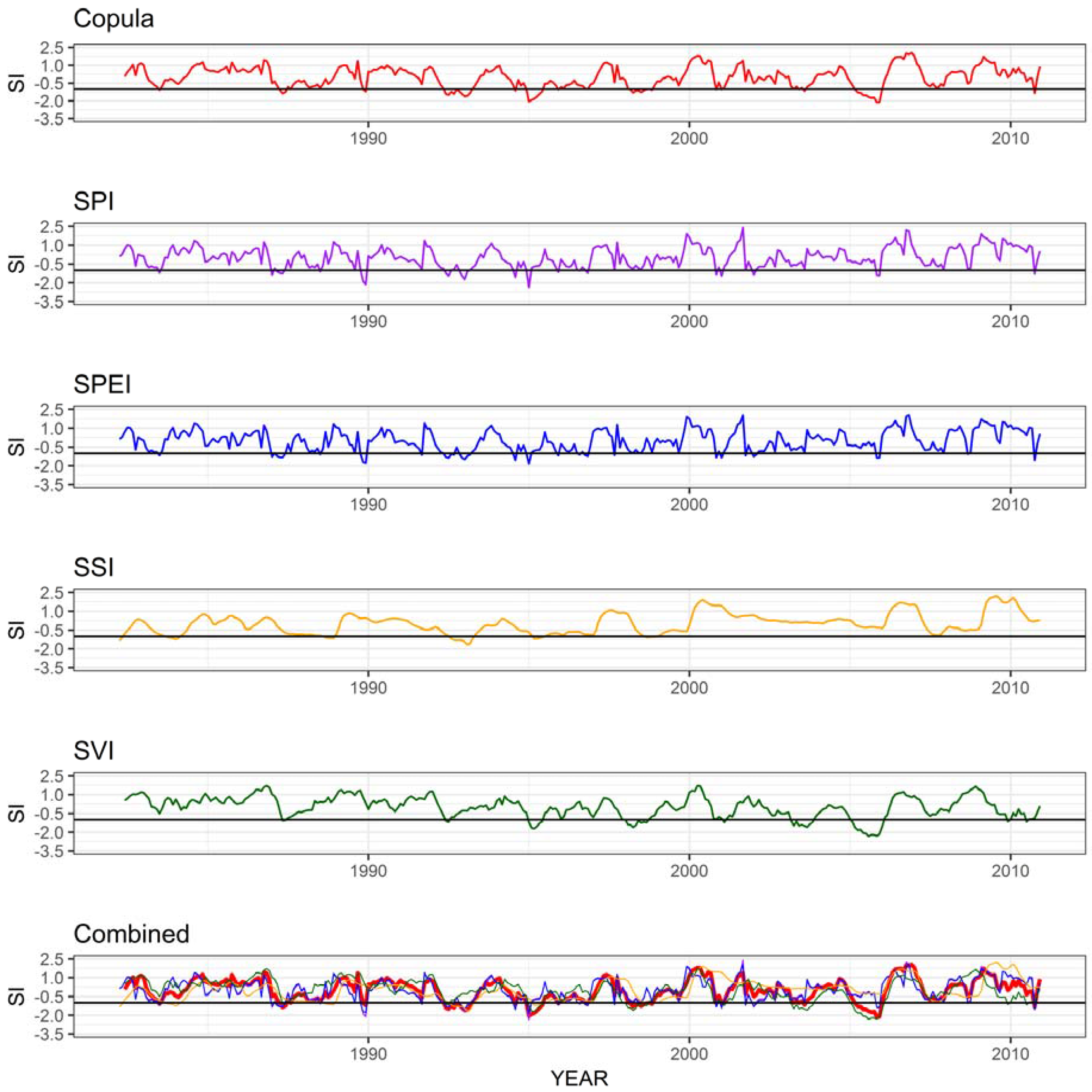
Every drought indicator was initially calculated as a standardized index of the 6-months running average. Figure 2 presents the temporal signal of the individual drought indicators, averaged over the entire basin. In addition, the copula time series is plotted that incorporates the SPEI, SSI, and SVI. Since SPI and SPEI correlate strongly (see Table 3), the SPI was not incorporated into the copula.
SPI and SPEI show almost an identical temporal signal. Solely, the extreme values of the SPI are surpassing the ones of the SPEI. Both indicators predict significant drought conditions between 1990 and 1995 and major wet periods between 2006 and 2010. The soil moisture-based SSI differs from the precipitation-based indicators. The data show less variation and only identify drought conditions in the 1980s and 1990s while after the year 2000 no droughts were recorded when considering the Basin’s mean. The vegetation conditions covered by the SVI show less variability compared to the precipitation-based indicators but still more than the SSI. It identifies drought conditions in the 1990s and mid-2000s with the most intense drought event in 2006. The resulting copula function incorporates characteristics of the individual indicators as can be seen in the lowest plot of Figure 2. The years 1995 and 2006 stand out as below –2 drought events. The recent years between 2006 and 2010 are rather wet, instead.
3.2. Threshold Variation
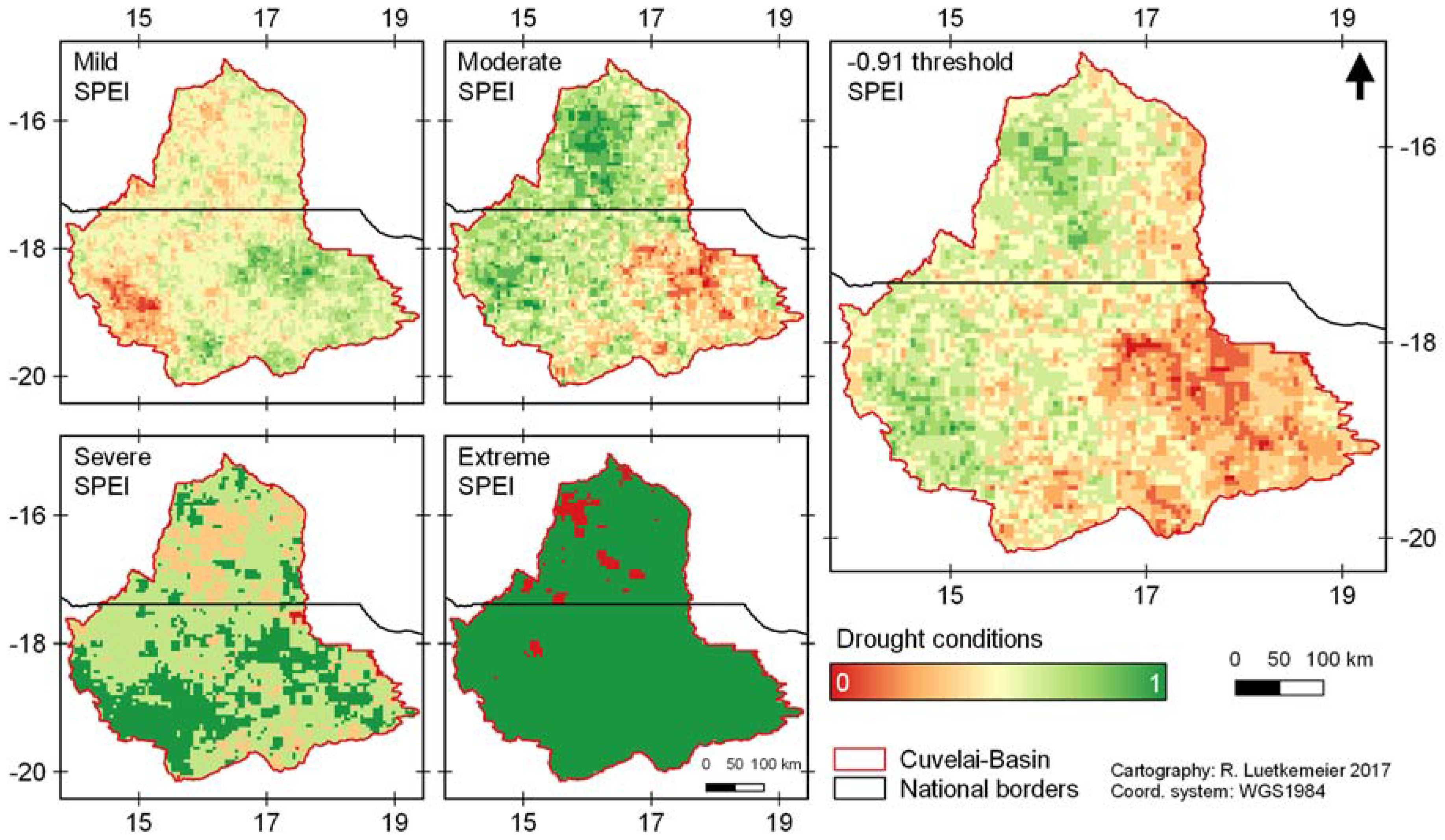
Identifying a drought event necessitates the selection of an appropriate threshold value. Commonly, –1 is chosen to distinguish dry conditions from a real drought event. However, the spatial pattern strongly varies with the selection of this threshold. The spatial analyses presented hereafter are based on the evaluation of the time series of April values, as these are regarded as giving the best estimation of drought conditions of the rainy season. Figure 3 exemplarily presents the results of the SPEI and shows the frequency of drought occurrence if different threshold values are considered. Herein, a mild drought is evident if the SPEI values range between 0 and –0.99, while extreme drought events are recorded if the SPEI shows values below –2.
The areas at risk of high drought frequencies vary strongly, with the southwest being the most affected region in terms of mild droughts, while the northwest in particular shows most extreme drought events. According to the National Drought Policy & Strategy, disaster droughts are declared in Namibia if the seasonal aggregates of a respective environmental parameter fall below the lowest 7% of the long-term average [87]. In the case of the SPEI, the threshold is then set to –0.91 which is depicted in Figure 3 and highlights the southeast as being the region of highest risk levels in terms of drought occurrence. For the purpose of consistency, this study applies the widely accepted –1 threshold value for further processing.
3.3. Spatial Drought Hot-Spots
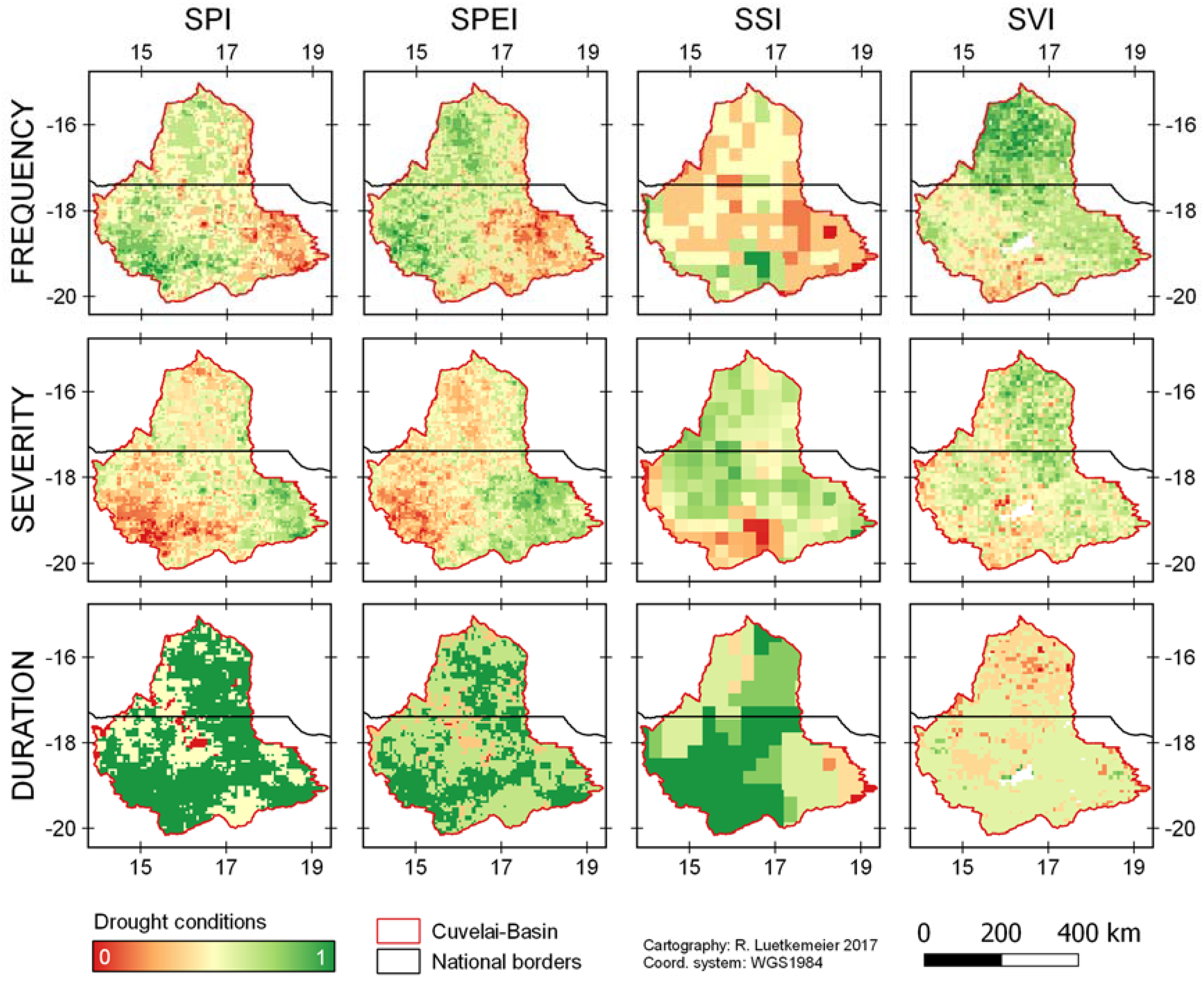
The frequency of occurrence is not the only important parameter to determine a drought. In this study, two more dimensions are regarded as being important for an overall drought hazard assessment. Figure 4 presents the results of each drought indicator, broken down into frequency of occurrence, severity, and duration.
It becomes obvious that the three dimensions depict different spatial characteristics of each indicator. While the frequency of occurrence is often estimated to be highest in the southeast (SPI & SPEI) and southwest (SVI), drought severity shows different results with a stronger focus on the southwest and south. Drought duration likewise highlights different areas. Here, the central and northwestern areas are threatened (SPI, SPEI, and SSI) and the northern part as well (SVI). Obviously, SPI and SPEI show similar patterns in all of the three dimensions, which is caused by the partly common database (CHIRPS 2.0). Due to their similarity, the SPI was excluded when applying the copula function to generate the BDI indicator.
3.4. Blended Drought Index
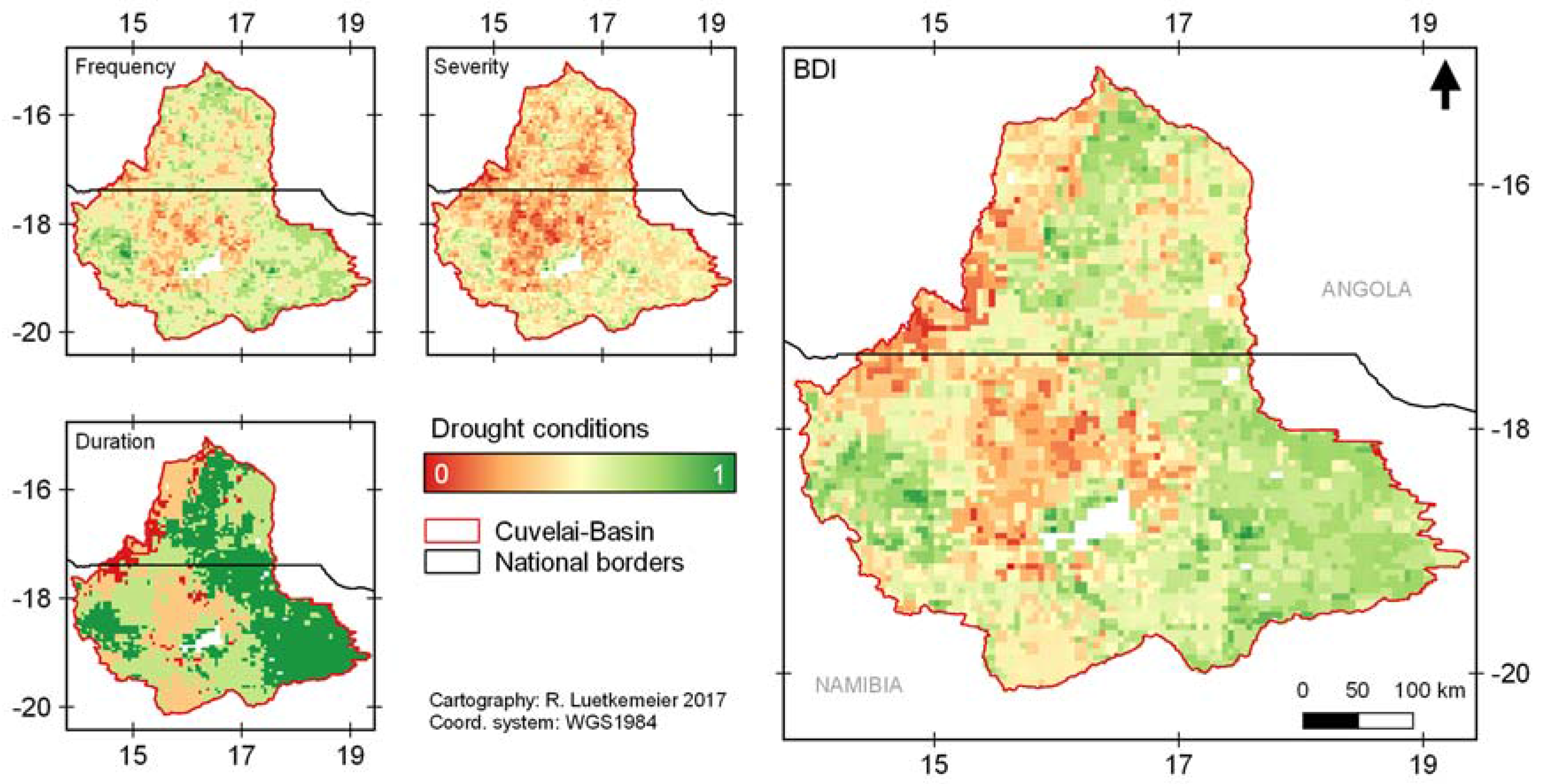
To generate an integrated drought hazard map for the Cuvelai-Basin, the BDI was derived from the copula that builds upon the SPEI, SSI, and VCI time series. In accordance with the other drought indicators, the April-values were selected for drought impact analysis and spatial representation.
Since all of the three dimensions are relevant for an integrated drought hazard map and analysis, the final BDI is generated as the average of frequency, severity, and duration, equally weighted and normalized. The resulting map depicted in Figure 5 clearly shows important drought hot-spot areas in the center, north of the Etosha Pan, and along the northwestern watershed boundary near the Kunene River.
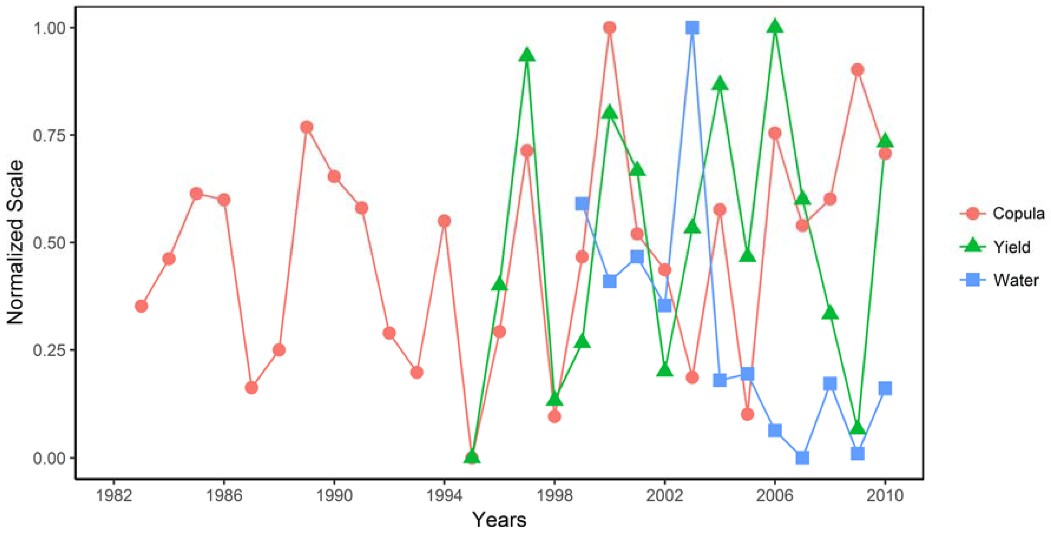
In order to evaluate the temporal drought signal of the copula, the frequency dimensions were averaged over the entire Basin and compared to millet/sorghum yield and water consumption data from central-northern Namibia. Figure 6 hence shows the normalized copula frequency values, with 1 indicating favorable and 0 unfavorable conditions in comparison with yield and water consumption. It becomes obvious that the yield data visually correlate well with the copula, except after the year 2006. The water consumption data should ideally work in an opposite direction according to the assumption that water consumption increases if drought conditions exist. From a visual interpretation, this is again true for most of the years except the period after 2006.
This visual impression is confirmed by the correlation analysis. Table 3 presents the Pearson and Spearman correlation coefficients of the drought indicators, including the copula, as well as yield and water consumption. The overall positive correlation of the copula with yield and the overall negative correlation with water consumption are confirmed and outperform the other indicators, in particular when considering the yield data.
4. Discussion
The study’s discussion section will focus on two key issues. First, the results will be reflected upon. Herein, the spatial drought signal will be discussed against the study’s target of developing an integrated drought hazard map. Furthermore, the temporal drought signals and their correlations with validation data will be analyzed. Second, the methodology will be discussed critically. Here, the selection of drought indicators, with a special focus on the copula approach used to combine the individual time series, will be evaluated against critical questions of seasonal comparability and threshold setting.
4.1. Reflection on Results
The main target of this study was the development of a drought hazard map that incorporates the drought’s impact on the social-ecological system in the Cuvelai-Basin. For this purpose, multiple drought indicators that are common tools for drought analysis (SPI, SPEI, SSI, and VCI) were combined. Their spatial dimensions, in particular the frequency of occurrence, however, show strongly diverging signals. Although each indicator is valid, it is difficult to decide which indicator to use for a drought hazard map in the study area. Against this background, the copula-based BDI incorporates the characteristics of the underlying indicators and even builds upon multiple dimensions (frequency of occurrence, severity, and duration). The resulting drought hazard map identifies hot-spot areas in the Basin, in particular the area north of the Etosha pan and the northwestern boundary of the Basin, near the Kunene River. These areas are threatened by drought events since these landscapes are highly degraded due to population density and intensive, uncontrolled grazing activities. Such human impacts are reflected in the SSI and SVI indicators and highlight the potential shortcomings of indicators that solely rely on precipitation. Since areas with a more dense vegetation cover are less threatened by scarce rainfalls and are moreover less vulnerable against drought effects like food and water insecurity, they may experience droughts in a meteorological sense but not in a social-ecological understanding. In this context not only can the frequency of occurrence and severity of droughts pose a problem but also consecutive (annual) droughts with recurring crop failures. These effects become apparent when comparing the results for the frequency and severity of meteorological droughts (see SPI and SPEI results in Figure 4) with the results for the BDI (Figure 5), where the former indicate major drought events in the southwest and southeast, which are offset in the BDI.
Temporally, all the indicators correlate well with the validation data of millet/sorghum yield and water consumption. The copula likewise reveals good results. While the period from 1995–2006 shows a good correlation, the subsequent years are less well correlated. This might be attributed to extraordinary wet conditions, in particular flooding events that might have led to yield reductions. Low water consumption from the tap network confirms this, assuming that the population was able to meet its water demand via traditional sources.
4.2. Reflection on Methodology
Drought indicators have been used for decades with an ever-increasing number of varieties. The use of copula functions to combine individual drought indicators has become prominent in recent years and more importantly has proved to reveal good results [42]. Hence, using a copula function in this study to link three individual drought indicators is regarded as an appropriate procedure for incorporating multiple drought effects into one single time series for further analysis. The selection of drought indicators, however, can be revisited. The suitability of further indicators can be evaluated in future research for the study area. Likewise, taking three dimensions into account such as the occurrence of droughts (frequency), the impact of single droughts (severity) as well as the impact of consecutive droughts (duration) can be a matter of discussion not only for their selection but also for their (in this case equal) weighting for the final index. Nonetheless, this approach highlights the matter’s complexity that should not be overlooked.
Due to the indicators’ shortcomings of being highly sensitive to low precipitation values in the case of SPI and SPEI for instance [51,81], the selection of the 6-months running mean April values as the rainy season’s aggregate is a rather new procedure. Comparing these values reveals direct insights into the status of the rainy season and makes it comparable over the years. The good correlation coefficients with yield and water consumption confirm the suitability of this procedure.
Section 3.2 described how the results of the SPEI indicator change if the threshold varies. The literature commonly sets the threshold to –1, while other thresholds can also be used to delineate drought events. It is thus important to point out that using a certain threshold will have a pronounced impact on the study results. The importance of threshold values should not be understated since they are necessary for clearly identifying emergency situations with all necessary relief measures associated to this. Nevertheless, the appropriate threshold value must be selected for every location, individually.
5. Conclusions
Drought is a recurring threat to Sub-Saharan Africa and the Cuvelai-Basin in Namibia and Angola, in particular. The current study seeks to shed light on the drought hazard itself with a focus on its temporal and spatial characteristics that are of relevance for the social-ecological system within the watershed. Based on insights from previous qualitative studies on drought impact in the target area, this study makes a contribution to characterizing the drought hazard in more detail. For this purpose, four commonly used drought indicators, the SPI, SPEI, SSI, and SVI (VCI) were used to construct a copula-based BDI that captures the effects of meteorological and agricultural droughts. The BDI can be presented as an integrated drought hazard map to depict hot-spot areas that are particularly threatened by drought events. Herein, drought frequency, severity, and duration are merged into one single indicator.
The drought hazard map is one important part of a comprehensive drought risk assessment. This includes further investigations on the vulnerability of the population living in the watershed. In the Cuvelai-Basin, most people practice subsistence agriculture and utilize traditional water sources which makes them highly sensitive to blue and green water scarcity. If droughts—as major hydro-climatic extreme events—occur, risk materializes in real disasters, as is currently happening in central-northern Namibia and many more places in Sub-Saharan Africa.
The study results will feed into an overall drought risk assessment at the household level, using a composite indicator, the Household Drought Risk Index (HDRI) that seeks to comprehensively characterize drought-prone households in the Cuvelai-Basin, to provide a better decision-base for respective governmental and non-governmental stakeholders.
Acknowledgments
This study was funded by the German Federal Ministry of Education and Research (BMBF) as part of the ‘Southern African Science Service Centre for Climate Change and Adaptive Land Management’ (SASSCAL) (task 016, Grant No. 01LG1201I).
Author Contributions
Robert Luetkemeier and Stefan Liehr conceived and designed the study. Robert Luetkemeier, Lina Stein and Lukas Drees performed data processing and analysis. All wrote the paper.
Conflicts of Interest
The authors declare no conflicts of interest.
References
- United Nations Secretariat of the International Strategy for Disaster Reduction (UNISDR). Drought Risk Reduction Framework and Practices. Contributing to the Implementation of the Hyogo Framework for Action; United Nations International Strategy for Disaster Reduction (UNISDR): Geneva, Switzerland, 2009. [Google Scholar]
- Collier, P.; Dercon, S. African agriculture in 50 years: Smallholders in a rapidly changing world? World Dev. 2014, 63, 92–101. [Google Scholar] [CrossRef]
- Cooper, P.J.M.; Dimes, J.; Rao, K.P.C.; Shapiro, B.; Shiferaw, B.; Twomlow, S. Coping better with current climatic variability in the rain-fed farming systems of sub-Saharan Africa: An essential first step in adapting to future climate change? Agric. Ecosyst. Environ. 2008, 126, 24–35. [Google Scholar] [CrossRef]
- Diao, X.; Hazell, P.; Thurlow, J. The role of agriculture in African development. World Dev. 2010, 38, 1375–1383. [Google Scholar] [CrossRef]
- Shiferaw, B.; Tesfaye, K.; Kassie, M.; Abate, T.; Prasanna, B.M.; Menkir, A. Managing vulnerability to drought and enhancing livelihood resilience in sub-Saharan Africa: Technological, institutional and policy options. Weather Clim. Extremes 2014, 3, 67–79. [Google Scholar] [CrossRef]
- Thornton, P.K.; Herrero, M. Adapting to climate change in the mixed crop and livestock farming systems in sub-Saharan Africa. Nat. Clim. Chang. 2015, 5, 830–836. [Google Scholar] [CrossRef]
- International Assessment of Agricultural Knowledge, Science and Technology for Development (IAASTD). Sub-Saharan Africa (SSA) Report; McIntyre, B.D., Herren, H.R., Wakhungu, J., Watson, R.T., Eds.; Agriculture at a crossroads; Island Press: Washington, DC, USA, 2009. [Google Scholar]
- Luetkemeier, R.; Liehr, S. Impact of drought on the inhabitants of the Cuvelai watershed: A qualitative exploration. In Drought: Research and Science-Policy Interfacing; Alvarez, J., Solera, A., Paredes-Arquiola, J., Haro-Monteagudo, D., van Lanen, H., Eds.; CRC Press/Balkema: Leiden, Netherlands, 2015; pp. 41–48. [Google Scholar]
- United Nations (UN). The Millennium Development Goals Report 2015; United Nations (UN): New York, NY, USA, 2015. [Google Scholar]
- UNECA; AU; ADB; UNDP. MDG Report 2015. Lessons Learned in Implementing the MDGs. Assessing Progress in Africa toward the Millennium Development Goals; United Nations Economic Commission for Africa (UNECA); African Union; African Development Bank; United Nations Development Programme (UNDP): Addis Ababa, Ethiopia, 2015. [Google Scholar]
- Handmer, J.; Honda, Y.; Kundzewicz, Z.W.; Arnell, N.; Benito, G.; Hatfield, J.; Mohamed, I.F.; Peduzzi, P.; Wu, S.; Sherstyukow, B.; et al. Changes in mpacts of climate extremes: Human systems and ecosystems. In Managing the Risks of Extreme Events and Disasters to Advance Climate Change Adaptation; Field, C.B., Barros, V., Stocker, T.F., Qin, D., Dokken, D.J., Ebi, K.L., Mastrandrea, M.D., Mach, K.J., Plattner, G.-K., Allen, S.K., et al., Eds.; A Special Report of Working Groups I and II of the Intergovernmental Panel on Climate Change (IPCC); Cambridge University Press: Cambridge, UK; New York, NY, USA, 2012; pp. 231–290. [Google Scholar]
- Seneviratne, S.I.; Nicholls, N.; Easterling, D.; Goodess, C.M.; Kanae, S.; Kossin, J.; Luo, Y.; Marengo, J.; McInnes, K.; Rahimi, M.; et al. Changes in climate extremes and their impacts on the natural physical environment. In Managing the Risks of Extreme Events and Disasters to Advance Climate Change Adaptation; Field, C.B., Barros, V., Stocker, T.F., Qin, D., Dokken, D.J., Ebi, K.L., Mastrandrea, M.D., Mach, K.J., Plattner, G.-K., Allen, S.K., et al., Eds.; A Special Report of Working Groups I and II of the Intergovernmental Panel on Climate Change (IPCC); Cambridge University Press: Cambridge, UK; New York, NY, USA, 2012; pp. 109–230. [Google Scholar]
- Gautam, M. Managing Drought in Sub-Saharan Africa: Policy Perspectives; The World Bank: Washington, DC, USA, 2006. [Google Scholar]
- Von Uexkull, N. Sustained drought, vulnerability and civil conflict in Sub-Saharan Africa. Political Geogr. 2014, 43, 16–26. [Google Scholar] [CrossRef]
- Mishra, A.K.; Singh, V.P. A review of drought concepts. J. Hydrol. 2010, 391, 202–216. [Google Scholar] [CrossRef]
- Wilhite, D.; Svoboda, M.; Hayes, M. Understanding the complex impacts of drought: A key to enhancing drought mitigation and preparedness. Water Resour. Manag. 2007, 21, 763–774. [Google Scholar] [CrossRef]
- Wilhite, D.A.; Glantz, M.H. Understanding: The drought phenomenon: The role of definitions. Water Int. 1985, 10, 111–120. [Google Scholar] [CrossRef]
- Kallis, G. Droughts. Annu. Rev. Environ. Resour. 2008, 33, 85–118. [Google Scholar] [CrossRef]
- Nalbantis, I.; Tsakiris, G. Assessment of hydrological drought revisited. Water Resour. Manag. 2008, 23, 881–897. [Google Scholar] [CrossRef]
- Tallaksen, L.M.; van Lanen, H.A.J. Hydrological Drought: Processes and Estimation Methods for Streamflow and Groundwater; Elsevier: Amsterdam, The Netherlands; Boston, MA, USA, 2004. [Google Scholar]
- Zelenhasić, E.; Salvai, A. A method of streamflow drought analysis. Water Resour. Res. 1987, 23, 156–168. [Google Scholar] [CrossRef]
- Mendelsohn, J.; Jarvis, A.; Robertson, T. A Profile and Atlas of the Cuvelai-Etosha Basin; Research and Information Services of Namibia (RAISON) & Gondwana Collection: Windhoek, Namibia, 2013. [Google Scholar]
- Hao, Z.; AghaKouchak, A. Multivariate standardized drought index: A parametric multi-index model. Adv. Water Resour. 2013, 57, 12–18. [Google Scholar] [CrossRef]
- Funk, C.; Peterson, P.; Landsfeld, M.; Pedreros, D.; Verdin, J.; Shukla, S.; Husak, G.; Rowland, J.; Harrison, L.; Hoell, A.; et al. The climate hazards infrared precipitation with stations—A new environmental record for monitoring extremes. Sci. Data 2015, 2, 150066. [Google Scholar] [CrossRef] [PubMed]
- Harris, I.; Jones, P.D.; Osborn, T.J.; Lister, D.H. Updated high-resolution grids of monthly climatic observations—The CRU TS3.10 Dataset. Int. J. Climatol. 2014, 34, 623–642. [Google Scholar] [CrossRef]
- Ek, M.B. Implementation of Noah land surface model advances in the National Centers for Environmental Prediction operational mesoscale Eta model. J. Geophys. Res. 2003, 108. [Google Scholar] [CrossRef]
- Pinzon, J.E.; Tucker, C.J. A non-stationary 1981–2012 AVHRR NDVI3g time series. Remote Sens. 2014, 6, 6929–6960. [Google Scholar] [CrossRef]
- Mendelsohn, J.; Weber, B. Cuvelai. The Cuvelai Basin Its Water and people in Angola and Namibia; Development Workshop: Luanda, Angola, 2011. [Google Scholar]
- Namibia Meteorological Service (NMS). Precipitation Data for Central-Northern Namibia (Unpublished); NMS: Windhoek, Namibia, 2013.
- EM-DAT International Disaster Database (EM-DAT), Centre for Research on the Epidemiology of Disasters (CRED). Available online: http://www.emdat.be/advanced_search/index.html (accessed on 26 July 2016).
- Namibia Statistics Agency (NSA). Namibia 2011. Population & Housing Census Main Report; Namibia Statistics Agency (NSA): Windhoek, Namibia, 2013; p. 214.
- Instituto Nacional de Estatistica (INE). Resultados Definitivos do Recenseamento Geral da Populacao e da Habitacao de Angola 2014; Instituto Nacional de Estatistica (INE): Luanda, Angola, 2016; p. 213.
- Freire-González, J.; Decker, C.; Hall, J.W. The economic impacts of droughts: A framework for analysis. Ecol. Econ. 2017, 132, 196–204. [Google Scholar] [CrossRef]
- Rockström, J. On-farm green water estimates as a tool for increased food production in water scarce regions. Phys. Chem. Earth Part. B Hydrol. Oceans Atmos. 1999, 24, 375–383. [Google Scholar] [CrossRef]
- Lavell, A.; Oppenheimer, M.; Diop, C.; Hess, J.; Lempert, R.; Li, J.; Muir_Wood, R.; Myeong, S. Climate Change: New Dimensions in Disaster Risk, Exposure, Vulnerability, and Resilience. In Managing the risks of extreme events and disasters to advance climate change adaptation; Field, C.B., Barros, V., Stocker, T.F., Qin, D., Dokken, D.J., Ebi, K.L., Mastrandrea, M.D., Mach, K.J., Plattner, G.-K., Allen, S.K., et al., Eds.; A Special Report of Working Groups I and II of the Intergovernmental Panel on Climate Change (IPCC); Cambridge University Press: Cambridge, UK; New York, NY, USA, 2012; pp. 25–64. [Google Scholar]
- Lloyd-Hughes, B. The impracticality of a universal drought definition. ResearchGate 2013, 117. [Google Scholar] [CrossRef]
- Pedro-Monzonís, M.; Solera, A.; Ferrer, J.; Estrela, T.; Paredes-Arquiola, J. A review of water scarcity and drought indexes in water resources planning and management. J. Hydrol. 2015, 527, 482–493. [Google Scholar] [CrossRef]
- Brown, M.E.; Brickley, E.B. Evaluating the use of remote sensing data in the U.S. Agency for International Development Famine Early Warning Systems Network. J. Appl. Remote Sens. 2012, 6, 063511-1. [Google Scholar] [CrossRef]
- Pulwarty, R.S.; Sivakumar, M.V.K. Information systems in a changing climate: Early warnings and drought risk management. Weather Clim. Extremes 2014, 3, 14–21. [Google Scholar] [CrossRef]
- Princeton Univeristy African Flood and Drought Monitor. Available online: http://stream.princeton.edu/AWCM/WEBPAGE/interface.php?locale=en (accessed on 16 December 2016).
- Naumann, G.; Dutra, E.; Barbosa, P.; Pappenberger, F.; Wetterhall, F.; Vogt, J.V. Comparison of drought indicators derived from multiple data sets over Africa. Hydrol. Earth Syst. Sci. 2014, 18, 1625–1640. [Google Scholar] [CrossRef]
- Mishra, A.K.; Singh, V.P. Drought modeling—A review. J. Hydrol. 2011, 403, 157–175. [Google Scholar] [CrossRef]
- AghaKouchak, A. A multivariate approach for persistence-based drought prediction: Application to the 2010–2011 East Africa drought. J. Hydrol. 2015, 526, 127–135. [Google Scholar] [CrossRef]
- Chang, J.; Li, Y.; Wang, Y.; Yuan, M. Copula-based drought risk assessment combined with an integrated index in the Wei River Basin, China. J. Hydrol. 2016, 540, 824–834. [Google Scholar] [CrossRef]
- Karamouz, M.; Rasouli, K.; Nazif, S. Development of a hybrid index for drought prediction: Case study. J. Hydrol. Eng. 2009, 14, 617–627. [Google Scholar] [CrossRef]
- McKee, T.B.; Doesken, J.; Kleist, J. The relationship of drought frequency and duration to time scales. In Proceedings of the 8th Conference on Applied Climatology, Anaheim, CA, USA, 17–22 January 1993; p. 1. [Google Scholar]
- World Meteorological Organization (WMO). Guidelines on Ensemble Prediction Systems and Forecasting; World Meteorological Organization: Geneva, Switzerland, 2012. [Google Scholar]
- Guttman, N.B. Accepting the Standardized Precipitation Index: A calculation algorithm1. JAWRA J. Am. Water Resour. Assoc. 1999, 35, 311–322. [Google Scholar] [CrossRef]
- Edwards, D.C.; McKee, T.B.; Doesken, N.J.; Kleist, J. Historical analysis of drought in the United States. In Proceedings of the Seventh Conference on Climate Variations, Long Beach, CA, USA, 2–7 February 1997; pp. 129–139. [Google Scholar]
- Stagge, J.H.; Tallaksen, L.M.; Gudmundsson, L.; Van Loon, A.F.; Stahl, K. Candidate distributions for climatological drought indices (SPI and SPEI). Int. J. Climatol. 2015, 35, 4027–4040. [Google Scholar] [CrossRef]
- Wu, H.; Svoboda, M.D.; Hayes, M.J.; Wilhite, D.A.; Wen, F. Appropriate application of the standardized precipitation index in arid locations and dry seasons. Int. J. Climatol. 2007, 27, 65–79. [Google Scholar] [CrossRef]
- Wu, H.; Hayes, M.J.; Wilhite, D.A.; Svoboda, M.D. The effect of the length of record on the standardized precipitation index calculation. Int. J. Climatol. 2005, 25, 505–520. [Google Scholar] [CrossRef]
- Wilks, D.S. Statistical Methods in the Atmospheric Sciences; Academic Press: Oxford, UK, 2011. [Google Scholar]
- Vicente-Serrano, S.M. Differences in spatial patterns of drought on different time scales: An analysis of the Iberian Peninsula. Water Resour. Manag. 2006, 20, 37–60. [Google Scholar] [CrossRef]
- Vicente-Serrano, S.M.; Beguería, S.; López-Moreno, J.I. A multiscalar drought index sensitive to global warming: The standardized precipitation evapotranspiration index. ResearchGate 2010, 23, 1696–1718. [Google Scholar] [CrossRef]
- Funk, C.C.; Peterson, P.J.; Landsfeld, M.F.; Pedreros, D.H.; Verdin, J.P.; Rowland, J.D.; Romero, B.E.; Husak, G.J.; Michaelsen, J.C.; Verdin, A.P. A Quasi-Global Precipitation Time Series for Drought Monitoring; Data Series; U.S. Geological Survey: Reston, VA, USA, 2014; p. 12. [CrossRef]
- Hessels, T.M. Comparison and Validation of Several Open Access Remotely Sensed Rainfall Products for the Nile Basin. Doctoral Dissertation, TU Delft, Delft University of Technology, Delft, The Netherlands, 2015. [Google Scholar]
- Tote, C.; Patricio, D.; Boogaard, H.; van der Wijngaart, R.; Tarnavsky, E.; Funk, C.C. Evaluation of satellite rainfall estimates for drought and flood monitoring in Mozambique. Remote Sens. 2015, 7, 1758–1776. [Google Scholar] [CrossRef]
- Ceccherini, G.; Ameztoy, I.; Hernández, C.P.R.; Moreno, C.C. High-resolution precipitation datasets in South America and West Africa based on satellite-derived rainfall, enhanced vegetation index and digital elevation model. Remote Sens. 2015, 7, 6454–6488. [Google Scholar] [CrossRef]
- Beguería, S.; Vicente-Serrano, S.M. Package “SPEI” 2015. Available online: https://cran.r-project.org/web/packages/SPEI/SPEI.pdf (accessed on 12 July 2017).
- McCarthy, T.S. Groundwater in the wetlands of the Okavango Delta, Botswana, and its contribution to the structure and function of the ecosystem. J. Hydrol. 2006, 320, 264–282. [Google Scholar] [CrossRef]
- Ekström, M.; Jones, P.D.; Fowler, H.J.; Lenderink, G.; Buishand, T.A.; Conway, D. Regional climate model data used within the SWURVE project—1: Projected changes in seasonal patterns and estimation of PET. Hydrol. Earth Syst. Sci. 2007, 11, 1069–1083. [Google Scholar] [CrossRef]
- Hassanein, M.K.; Kahlil, A.A.; Essa, Y.H. Assessment of drought impact in Africa using Standard Precipitation Evapotranspiration Index. Nat. Sci. 2013, 11, 75–81. [Google Scholar] [CrossRef]
- McEvoy, D.J.; Huntington, J.L.; Abatzoglou, J.T.; Edwards, L.M. An evaluation of multiscalar drought indices in Nevada and eastern California. Earth Interact. 2012, 16, 1–18. [Google Scholar] [CrossRef]
- Yu, M.; Li, Q.; Hayes, M.J.; Svoboda, M.D.; Heim, R.R. Are droughts becoming more frequent or severe in China based on the Standardized Precipitation Evapotranspiration Index: 1951–2010? Int. J. Climatol. 2014, 34, 545–558. [Google Scholar] [CrossRef]
- Chen, F.; Mitchell, K.; Schaake, J.; Xue, Y.; Pan, H.-L.; Koren, V.; Duan, Q.Y.; Ek, M.; Betts, A. Modeling of land surface evaporation by four schemes and comparison with FIFE observations. J. Geophys. Res. Atmos. 1996, 101, 7251–7268. [Google Scholar] [CrossRef]
- Sheffield, J.; Goteti, G.; Wen, F.; Wood, E.F. A simulated soil moisture based drought analysis for the United States. J. Geophys. Res. Atmos. 2004, 109, D24108. [Google Scholar] [CrossRef]
- Delignette-Muller, M.L.; Dutang, C.; Pouillot, R.; Denis, J.-B. Package “fitdistrplus” 2016. Available online: https://cran.r-project.org/web/packages/fitdistrplus/fitdistrplus.pdf (accessed on 12 July 2017).
- Kogan, F.N. Application of vegetation index and brightness temperature for drought detection. Adv. Space Res. 1995, 15, 91–100. [Google Scholar] [CrossRef]
- Dutta, D.; Kundu, A.; Patel, N.R.; Saha, S.K.; Siddiqui, A.R. Assessment of agricultural drought in Rajasthan (India) using remote sensing derived Vegetation Condition Index (VCI) and Standardized Precipitation Index (SPI). Egypt. J. Remote Sens. Space Sci. 2015, 18, 53–63. [Google Scholar] [CrossRef]
- Quiring, S.M.; Ganesh, S. Evaluating the utility of the Vegetation Condition Index (VCI) for monitoring meteorological drought in Texas. Agric. For. Meteorol. 2010, 150, 330–339. [Google Scholar] [CrossRef]
- Unganai, L.S.; Kogan, F.N. Drought monitoring and corn yield estimation in southern Africa from AVHRR Data. Remote Sens. Environ. 1998, 63, 219–232. [Google Scholar] [CrossRef]
- Gudmundsson, L.; Stagge, J.H. Package “SCI” 2016. Available online: https://cran.r-project.org/web/packages/SCI/SCI.pdf (accessed on 12 July 2017).
- Kao, S.-C.; Govindaraju, R.S. A copula-based joint deficit index for droughts. J. Hydrol. 2010, 380, 121–134. [Google Scholar] [CrossRef]
- Saghafian, B.; Mehdikhani, H. Drought characterization using a new copula-based trivariate approach. Nat. Hazards 2014, 72, 1391–1407. [Google Scholar] [CrossRef]
- Favre, A.-C.; El Adlouni, S.; Perreault, L.; Thiémonge, N.; Bobée, B. Multivariate hydrological frequency analysis using copulas: Multivariate frequency analysis using copulas. Water Resour. Res. 2004, 40. [Google Scholar] [CrossRef]
- Sklar, A. Fonctions de répartition à n dimension e leurs marges. Publ. Inst. Stat. Univ. Paris 1959, 8, 229–231. [Google Scholar]
- Yan, J. Enjoy the joy of copulas: With a package copula. J. Stat. Softw. 2007, 21, 1–21. [Google Scholar] [CrossRef]
- Nelson, R.B. An Introduction to Copulas; Springer Series in Statistics; Springer: New York, NY, USA, 2006. [Google Scholar]
- Mendelsohn, J.M.; El Obeid, S.; Roberts, C.; Namibia Ministry of Environment and Tourism. A Profile of North-Central Namibia; Gamsberg Macmillan Publishers: Windhoek, Namibia, 2000.
- Spinoni, J.; Naumann, G.; Carrao, H.; Barbosa, P.; Vogt, J. World drought frequency, duration, and severity for 1951–2010: World Drought Climatologies for 1951-2010. Int. J. Climatol. 2014, 34, 2792–2804. [Google Scholar] [CrossRef]
- Halwatura, D.; Lechner, A.M.; Arnold, S. Drought severity–duration–frequency curves: A foundation for risk assessment and planning tool for ecosystem establishment in post-mining landscapes. Hydrol. Earth Syst. Sci. 2015, 19, 1069–1091. [Google Scholar] [CrossRef]
- Ministry of Agriculture, Water and Forestry (MAWF). Agricultural Statistics Bulletin; Ministry of Agriculture, Water and Forestry (MAWF): Windhoek, Namibia, 2011.
- Ministry of Agriculture, Water and Forestry (MAWF). Agricultural Statistics Bulletin; Ministry of Agriculture, Water and Forestry (MAWF): Windhoek, Namibia, 2005.
- Ministry of Agriculture, Water and Forestry (MAWF). Agricultural Statistics Bulletin; Ministry of Agriculture, Water and Forestry (MAWF): Windhoek, Namibia, 2009.
- Namibia Water Corporation (NamWater). Tap Water Consumption Data of Central-Northern Namibia from 1995 to 2013 (Unpublished); Namibia Water Corporation (NamWater): Windhoek, Namibia, 2014. [Google Scholar]
- Republic of Namibia. National Drought Policy & Strategy; National Drought Task Force, Republic of Namibia: Windhoek, Namibia, 1997.
Figure 1.
Cuvelai-Basin in Angola and Namibia.

Figure 2.
Drought indicators as standardized 6-months running averages of the entire Basin. The solid horizontal line indicates the threshold value of –1. SPI = Standardized Precipitation Index, SPEI = Standardized Precipitation Evapotranspiration Index, SSI = Standardized Soil Moisture Index, SVI = Standardized Vegetation Index.

Figure 3.
Drought index threshold variation for Cuvelai-Basin. Maps show the frequency of drought occurrence on a normalized scale from 0 (often) to 1 (rare) depending on the drought threshold chosen. Exemplarily, the SPEI indicator was chosen for illustration. Mild (0 to –0.99), Moderate (–1 to –1.49), Severe (–1.5 to –1.99) and Extreme (<–2) droughts are distinguished from the official Namibian drought threshold based on the lowest 7% quantile.

Figure 4.
Drought indicator dimensions of frequency of occurrence, severity and duration, for the Cuvelai-Basin. The results are represented spatially on a normalized scale from 0 (unfavorable) to 1 (favorable). White pixels within the Basin are the result of “no-data” pixels from the initial NDVI vegetation dataset.

Figure 5.
Spatial representation of the copula, for the Cuvelai-Basin. Beside frequency of occurrence, severity and duration, the BDI itself is presented as the average of the individual dimensions on a pixel-basis.
Figure 5.
Spatial representation of the copula, for the Cuvelai-Basin. Beside frequency of occurrence, severity and duration, the BDI itself is presented as the average of the individual dimensions on a pixel-basis.

Figure 6.
Temporal copula frequency signal in comparison with the validation datasets of millet/sorghum yield and water consumption from central-northern Namibia. The time series were normalized from 0 (copula: unfavorable, yield: low, water consumption: low) to 1 (copula: favorable, yield: high, water consumption: high).


Table 1.
Datasets used to calculate the drought indices.
| Parameter | Dataset | Spat. Cov. | Spat. Res. | Temp. Cov. | Temp. Res. | Provider | Reference |
|---|---|---|---|---|---|---|---|
| Precipitation | CHIRPS 2.0 | 50° N–50° S | 0.05° | 1981–2015 | monthly | UCSB, CHG | [24] |
| Evapotranspiration | CRU TS3.23 | global | 0.5° | 1901–2013 | monthly | UEA, CRU | [25] |
| Soil Moisture | GLDAS | global | 0.25° | 1980–2010 | monthly | NASA | [26] |
| Vegetation | NDVI3g | global | 0.08° | 1981–2013 | 15 days | GIMMS | [27] |
(UCSB = University of California, Santa Barbara, CHG = Climate Hazards Group, UEA = University of East Anglia, CRU = Climate Research Unit, NASA = National Aeronautics and Space Administration).
Table 2.
Drought intensities according to the size of standard deviation [46].
Table 2.
Drought intensities according to the size of standard deviation [46].
| SPI Values | Drought Severity |
|---|---|
| 0 to –0.99 | Mild drought |
| –1.00 to –1.49 | Moderate drought |
| –1.50 to –1.99 | Severe drought |
| <–2.00 | Extreme drought |
Table 3.
Pearson and Spearman correlations between the drought indicators, millet/sorghum yield, and rural water consumption in central-northern Namibia.
Table 3.
Pearson and Spearman correlations between the drought indicators, millet/sorghum yield, and rural water consumption in central-northern Namibia.
| Copula | SPI | SPEI | SSI | SVI | ||||||
|---|---|---|---|---|---|---|---|---|---|---|
| P | S | P | S | P | S | P | S | P | S | |
| Copula | ||||||||||
| SPI | *** 0.86 | *** 0.87 | ||||||||
| SPEI | *** 0.86 | *** 0.87 | *** 1.00 | *** 1.00 | ||||||
| SSI | *** 0.77 | *** 0.70 | *** 0.63 | ** 0.54 | *** 0.62 | ** 0.55 | ||||
| SVI | *** 0.81 | *** 0.78 | ** 0.50 | ** 0.56 | ** 0.51 | ** 0.56 | * 0.35 | * 0.36 | ||
| Yield | * 0.51 | * 0.56 | * 0.43 | * 0.50 | * 0.46 | * 0.50 | * 0.46 | * 0.48 | 0.35 | 0.16 |
| Water | –0.45 | * –0.52 | –0.45 | –0.42 | –0.45 | –0.42 | –0.31 | –0.38 | –0.30 | –0.17 |
* p < 0.1, ** p < 0.01, *** p < 0.001, P = Pearson-r, S = Spearman-r. Bold coefficients indicate strongest correlations.
© 2017 by the authors. Licensee MDPI, Basel, Switzerland. This article is an open access article distributed under the terms and conditions of the Creative Commons Attribution (CC BY) license (http://creativecommons.org/licenses/by/4.0/).
Share and Cite
MDPI and ACS Style
Luetkemeier, R.; Stein, L.; Drees, L.; Liehr, S. Blended Drought Index: Integrated Drought Hazard Assessment in the Cuvelai-Basin. Climate 2017, 5, 51. https://0-doi-org.brum.beds.ac.uk/10.3390/cli5030051
AMA Style
Luetkemeier R, Stein L, Drees L, Liehr S. Blended Drought Index: Integrated Drought Hazard Assessment in the Cuvelai-Basin. Climate. 2017; 5(3):51. https://0-doi-org.brum.beds.ac.uk/10.3390/cli5030051
Chicago/Turabian StyleLuetkemeier, Robert, Lina Stein, Lukas Drees, and Stefan Liehr. 2017. "Blended Drought Index: Integrated Drought Hazard Assessment in the Cuvelai-Basin" Climate 5, no. 3: 51. https://0-doi-org.brum.beds.ac.uk/10.3390/cli5030051
Note that from the first issue of 2016, this journal uses article numbers instead of page numbers. See further details here.