
Influence of Atmospheric Circulation on the Baltic Sea Level Rise under the RCP8.5 Scenario over the 21st Century

Institute of Coastal Research, Helmholtz-Zentrum Geesthacht, Max-Planck-Str. 1, 21502 Geesthacht, Germany
Climate 2017, 5(3), 71; https://0-doi-org.brum.beds.ac.uk/10.3390/cli5030071
Submission received: 1 August 2017
/
Revised: 31 August 2017
/
Accepted: 1 September 2017
/
Published: 6 September 2017
Abstract
:This study aims to estimate the influence of atmospheric circulation modes on future Baltic Sea level rise under the Representative Concentration Pathway 8.5 (RCP8.5) climate scenario for the period 2006–2100. For this estimation, the connection between the sea level variations in two selected representative locations—Stockholm and Warnemünde, and two atmospheric indices—the Baltic Sea and North Sea Oscillation (BANOS) index and the North Atlantic Oscillation (NAO) index is statistically analysed. Correlations of winter means between atmospheric indices, BANOS and NAO, and tide gauges are measured as 0.85 and 0.55 for Stockholm, and 0.55 and 0.17 for Warnemünde over the period 1900–2013. Assuming that the established connection remains unchanged, the influence of atmospheric circulation modes on future Baltic Sea level rise is estimated from the projections of atmospheric indices, which are constructed from the SLP outputs of climate models participating in phase 5 of the Coupled Model Intercomparison Project (CMIP5) under the RCP8.5 scenario. The main conclusion is that the contribution of those atmospheric modes to the Baltic Sea level rise is likely to remain small over the 21st century. Additionally, corresponding trend estimations of model realizations indicate the large influence of the internal climatic variability of the CMIP5 models on those future trends. One of the most important findings of this study is that anthropogenic forcing does not play a key role in the evolution of these atmospheric indices.
1. Introduction
The main purpose of this study is to estimate the contribution of atmospheric circulation to future Baltic Sea level rise under the RCP8.5 scenario over the 21st century. For this estimation, sea level pressure (SLP) outputs of eight models participating in the Coupled Model Intercomparison Project Phase 5 (CMIP5), the Baltic Sea and North Sea Oscillation (BANOS) index, the North Atlantic Oscillation (NAO) index, and the sea level records from the Stockholm and Warnemünde tide gauges are used on interannual time scales. Additionally, considering the fact that the effect of large-scale air temperature may cause modifications in the pattern of atmospheric circulation, the connection in multidecadal trends between the atmospheric indices, and the extended North Atlantic/Europe region air temperature is also investigated in this study. A possible connection between those variables would indicate the existence of a global warming signal in the related modes of atmospheric circulation, hence, would modify the BANOS and NAO indices.
Global warming causes the global mean sea level to rise mainly due to the thermal expansion of the water and melting of land-locked ice. However, regional sea level trends deviate substantially from those of global means [1]. Thus, estimating the sea-level variability in some regions requires studies focused on revealing the impact of the individual driving factors on sea-level variability [2,3,4]. For instance, Grinsted et al. [5] explored the sea-level rise projections in Northern Europe including the Baltic Sea under the Representative Concentration Pathway 8.5 (RCP8.5) scenario. Considering the regional fingerprints of some major sea level components of the global sea level budget like ocean thermal expansion, melting/dynamics of glaciers, ice loss from the Greenland and Antarctic ice sheets, and changes in land water storage, their best estimation of relative sea-level rise is 0.25 m for Stockholm under the RCP8.5 scenario over the 21st century. However, projections of global mean sea level rise for the RCP8.5 scenario are in the range between 0.52 and 0.98 m over the 21st century [1].
Besides, it is known that the most important factors causing sea level variations in the Baltic Sea from interannual to decadal time scales are connected to the variability of atmospheric circulation [6,7,8]. Therefore, modifications in the atmospheric conditions are important driving factors for understanding the possible sea-level rise in the near future, especially in the regions like the Baltic Sea, where the variability of sea level is quite sensitive to atmosphere driven boundary conditions, such as wind, air pressure, air temperature, and freshwater flux [9,10,11]. Since the NAO can carry information about large scale changes in the pressure field, wind field, heat fluxes, and freshwater fluxes, there are several studies investigating the link between the NAO and sea-level variability in the Baltic Sea [8,12]. Two main conclusions on that link are that the NAO has a heterogeneous effect on the sea-level variability in the spatial domain and that this link is also not stable in time [11].
By analyzing the winter monthly means of sea level and SLP patterns, Heyen et al. [13] established a statistical link between the leading vectors of those variables which are described by a canonical correlation analysis (CCA). They detected a strong connection between an individual mode of large-scale SLP and the sea level variation pattern in the Baltic Sea region. They concluded that wind stress over the transition area (covering the Skagerrak, the Kattegat, and the Danish Straits), inverse barometric effect (IBE), and sea level variation in the German Bight are associated with the leading sea level CCA vector in the Baltic Sea. However, they did not find any considerable contribution of the precipitation to that leading mode of sea level variation.
More recently, Hünicke and Zorita [8] investigated the role of atmospheric factors such as three-to-five leading vectors of large-scale SLP, sea surface temperature, and precipitation in the Baltic Sea level variations by establishing a statistical model between the individual tide gauges and those variables (stepwise multivariate regression) on interannual time scales. By filtering time series with 11-year running means, they first showed that a non-negligible amount of sea-level variability cannot be linearly explained by the SLP field. Following this preliminary result, they detected spatially heterogeneous contributions of precipitation and temperature to Baltic Sea level variability. Further analysis is applied by Hünicke et al. [14] on a decadal time series of winter means. They confirmed that the impact of atmospheric forcing on decadal sea-level variability is also geographically heterogeneous in the Baltic Sea region. Hünicke et al. [14] found that sea-level variability in the southern Baltic can be better explained by spatially averaged precipitation; besides, atmospheric circulation patterns are dominant factors in modifying sea level variations in the central, eastern, and northern Baltic Sea on decadal time scales. However, temperature does not play a role in causing variation in the Baltic Sea level on decadal time scales, in contrast to the results of Hünicke and Zorita [8]. It can be the case that the strength of the relation between sea level and a climatic factor becomes important due to the fact that the mean state of the system can be changed slowly on decadal time scales, as that was likely the case for the different impact of temperature on sea level between the studies Hünicke and Zorita [8] and Hünicke et al. [14]. Those results of Hünicke and Zorita [8] and Hünicke et al. [14] also seem to be contradictive in comparison to the study of Heyen et al. [13], which did not detect a considerable effect of precipitation on sea level variability in the Baltic Sea. This discrepancy may mainly arise from the fact that Heyen et al. [13] used a CCA-method by using principal components of sea level and of SLP field, which cannot capture the effects that are not large-scale and spatially incoherent over the whole Baltic Sea region.
Further investigating the link between the regional sea level, including off-shore observations and large-scale atmospheric circulation, Karabil et al. [15] suggested a new atmospheric index (BANOS) explaining locally up to 90% of the interannual sea-level variance in the Baltic Sea region in wintertime. They constructed the BANOS index from the difference of two normalized SLP centres of action located over (5° W, 45° N) and (20° E, 70° N), which is distinct from the standard NAO SLP pattern in wintertime. Their investigation also showed that the BANOS mode of atmospheric circulation is connected more strongly and steadily over time to sea-level variability in the Baltic Sea and to the North Sea, in comparison to the NAO over the period 1900–2013. In addition, that atmospheric pattern is connected more homogeneously to the whole Baltic Sea level variability than the first 5 major modes of atmospheric circulation (including NAO). Notably they described that the IBE and net energy flux strongly contribute to the connection between the BANOS index and sea level, but the precipitation contribution to that connection is negligible in wintertime.
Concerning the future projections of the Baltic Sea level rise driven by atmospheric factors, Hünicke [16] analysed the contribution of SLP and precipitation to the future sea level changes in the Baltic Sea based on decadal winter means. Using SLP and precipitation outputs from five different Coupled Model Intercomparison Project phase three (CMIP3) climate model simulations driven by the A2 scenario, that study projected the contribution of these two atmospheric factors to sea-level rise through the 21st century for wintertime. That projection was based on the link between those two atmospheric factors and sea level established by Hünicke et al. [14]. It was suggested that although the SLP outputs of three climate models caused statistically significant sea level rise in the central and eastern Baltic Sea, all analysed models indicate that precipitation will cause significant sea level trends in the southern Baltic Sea.
Recently, using different contributors including meteorological drivers on sea level trends along the Finnish coast, Johansson et al. [17] projected the sea level rise based on the CMIP3 simulations. Investigating the connections of the NAO index and the zonal component of the geostrophic wind to sea level variability, they found that 37–46% of sea level variance can be explained by the NAO index, but the zonal geostrophic wind explains 84–89% of the variance of sea level on interannual time scales. Based on this connection between zonal geostrophic wind and sea-level variability, they estimated long-term mean sea level trend in the Finnish coast driven by changes in the atmospheric circulation ranging from a 4 cm sink to a 19 cm rise by 2100.
Moreover, it is documented that large-scale sea-surface-temperature (SST) variations may play a key role in modulating the modes of atmospheric circulation in the North Atlantic, in particular the NAO [18,19]. It is therefore possible that a mode of atmospheric variability in the North Atlantic can be slowly directed by the multidecadal evolution of the SST [20]. Considering that possible modifications in atmospheric modes such as NAO can influence the climate in the Northern Europe climate, especially in winter, Cattiaux and Cassou [21] revisited the potential effect of warming trends due to the increase in greenhouse gas (GHG) emissions on individual modes of atmospheric circulation. They compared the trends in the NAO as simulated in the CMIP3 A2 scenario with the CMIP5 RCP8.5 scenario over the 21st century. They found that, although the CMIP3 simulations indicate positive trends in the NAO, no trend is indicated by the CMIP5 simulations. The conclusions of Cattiaux and Cassou [21] are important for understanding and verifying the possible projections of the atmosphere-driven sea-level variability in the Baltic Sea region.
To sum up, climate-induced change in modes of atmospheric circulation can substantially modify sea-level rise in the Baltic Sea. The findings suggest that some climatic factors such as the IBE, zonal component of the geostrophic wind, net energy flux, precipitation, air temperature, and downwelling along the coast of German Bight are contributing to mean sea-level variability in the Baltic Sea. This study uses two different atmospheric modes that encapsulate a lot of information about wind, IBE, air temperature, downwelling along the east coast of the North Sea, and freshwater flux regarding the Baltic Sea level variability. The main climatic factors contributing to the connections between those indices and Baltic Sea level variability are the IBE attributed to BANOS pattern and zonal geostrophic wind attributed to NAO pattern. In addition, corresponding modes of the atmospheric circulation can be slowly directed by SST trends due to the increase in GHG emissions. However, there are only few studies that have investigated the effect of future circulation changes on sea level in the Baltic Sea area [22]. To the author’s knowledge, there is no study focused on the contribution of atmospheric forcing to future Baltic Sea level rise using the state-of-the-art CMIP5 model outputs.
In this study, the skill of the CMIP5 models by simulating the present variations is initially tested. Therefore, the first analysis step of this study was on how well the CMIP5 models simulate present-day climatology of the SLP over the Baltic Sea and North Sea regions. The rationale behind this test was to define whether a plausible estimation of future sea level changes based on simulation outputs of those climate models is possible for the Baltic Sea. In the second step, a linear connection between atmospheric indices (NAO and BANOS) and sea level, the Stockholm and Warnemünde tide gauges, is established. Based on that connection, the skill of the associated statistical model is also analysed in order to understand whether the statistical model is good enough to establish the connection between the modes of the atmospheric circulation and sea level variability. After those two critical tests, the main investigation of this study is carried out to estimate the rate of Baltic Sea level rise due to changes in the atmospheric circulation under the RCP8.5 scenario over the 21st century. An additional goal was to quantify the variations of the simulated atmospheric trends that are due to internal climate variability. In the last step, the effect of large-scale air temperature on relevant modes of atmospheric circulation is investigated by using multidecadal trend variations. A significant relationship between those two variables would indicate the existence of a global warming signal in the long-term evolution of atmospheric circulation modes. Since the field mean of large-scale SST over the North Atlantic, which may control the phase of BANOS or NAO, is expected to represent the SST signal at global scale.
This study is restricted to the winter season. In this season, the variability of atmospheric circulation is largest. It enables the current study to better understand the influence of atmospheric circulation on the Baltic Sea level variation by increasing the signal-to-noise ratio, which primarily decreases due to the local processes and measurement noises.
The structure of this study is organized as follows: the second section explains the data used in this study. The following section outlines the applied methods on the analysis of the data sets. The results are presented in Section 4. Section 5 discusses the results and Section 6 concludes the manuscript.
2. Data Sets
Winter (December-to-February) means of following data sets were used in this study.
2.1. Sea Level Observations
Winter means of the Stockholm and Warnemünde tide gauges are used to establish a statistical connection between the Baltic Sea level and atmospheric indices over the period 1900–2013. These stations are representative of Baltic Sea level variability on interannual and longer time scales [6,8,23]. The stations are located in the central and southern parts of the Baltic Sea. The observations are provided by Permanent Service for Mean Sea Level [24] and Ekman [25] long-term sea level records. A map showing the locations of the tide gauges, including the sea-level trend estimations due to the considered atmospheric indices is provided in the Results section.
2.2. Climatic Data
2.2.1. SLP Data
There are two types of SLP data used in this study.
First, 30-year SLP means of reanalysis and CMIP5 [26] model outputs are compared by selecting the period 1971–2000. The model outputs were yielded from the historical run outputs of eight CMIP5 models and the SLP reanalysis data provided by National Centers for Environmental Prediction (NCEP)/National Center for Atmospheric Research (NCAR) [27]. The meteorological reanalysis assimilates different observations into a weather prediction model and produces a complete grid data set over the whole period. This data set has a spatial resolution of 192 × 94 points with T62 Gaussian grid covering the Earth’s surface.
Second, the SLP outputs from eight different CMIP5 models [26] are used to project the variability of two atmospheric indices, BANOS and NAO, over the 21st century. Three realizations (r1i1p1, r2i1p1, r3i1p1) for each model were used in this study from the RCP8.5 scenario. The criterion behind this selection was to investigate the influence of internal climatic variability of the CMIP5 models on the projected Baltic Sea level trends. The detailed information on the CMIP5 models is given in Table 1.
As mentioned above, the SLP outputs of those models were used in order to project modes of the atmospheric variations under the RCP8.5 scenario. RCP 8.5 was developed using the MESSAGE model and the Integrated Assessment Framework by the International Institute for Applied Systems Analysis (IIASA), explained in Riahi et al. [28]. The RCP8.5 scenario is a concentration pathway with the highest defined rates of GHG emissions. This scenario consists of assumptions that there will be high population and a relatively slow income growth, with modest rates of technological change, and energy intensity improvements. In the long term, this will lead to high energy demand and GHG emissions in the absence of climate change policies. Like the other RCPs, the RCP8.5 is named based on the radiative forcing value in the year 2100 relative to the pre-industrial value, +8.5 W/m2 [29]. Since it is assumed that the reader is familiar with the climate scenarios, this study does not provide information on the RCP8.5 scenario in detail.
2.2.2. Atmospheric Indices
There are two atmospheric indices used in this study.
One of those indices was the BANOS index [15], which is consistently well correlated over time to Baltic Sea level variability. This construction was carried out by using the difference between the normalized SLP fields, provided by the National Centre for Atmospheric Research (NCAR) [30], over the geographical points (5° W, 45° N) and (20° E, 70° N). These two grid-cells are fixed, and define the BANOS index for the period 1900–2013.
The second one was the NAO index, which represents a pattern of the large-scale pressure fields over the North Atlantic region. The time-varying intensity of this pattern can be summarised by the NAO index. The monthly time series of the NAO index was provided by Hurrell et al. [31]. They constructed the NAO index by using the differences between normalized anomalies of two sea level pressure stations: Lisbon, Portugal, and Reykjavik, Iceland. Normalization is required in order to filter out the series being dominated by the larger variability of the northern station in comparison to variability of the southern station [32].
2.2.3. Surface Air Temperature
The surface air temperature outputs of those CMIP5 models, as provided by Taylor et al. [26], covering the extended North Atlantic region (Area limits: 90° E to 50° W and 20° N to 80° N) are also used in this study.
3. Methods
This section concerns the applied methods in this study, and is classified into three parts.
3.1. Method for Model Assessment
As was mentioned previously, 30-year SLP means of reanalysis and CMIP5 model outputs are compared by selecting the period 1971–2000, which is a standard reference period in climatology in order to characterize present normal climate conditions over a certain area. The goal of this comparison was to assess the model performance in simulating the present-day SLP climatology. Since this comparison requires the same grid structure with the same resolution, all SLP grids of each model are interpolated onto the regular NCEP 2.5° × 2.5° grid by using bilinear interpolation prior to the assessment of the climate models. The selected region covers the geographical area between (20° W–37.5° E) longitudes and (47.5° N–70° N) latitudes.
Afterwards, the skill of the considered CMIP5 climate models in simulating the present-day SLP climatology is evaluated. For this evaluation, respective spatial standard deviations of the spatial SLP means, and the correlations and root-mean-square (RMS) differences of those SLP fields between the reanalysis and the models are computed. To represent the results, the Taylor diagram [33], which graphically summarizes the similarity of the climate models with respect to a reference data set, is used. Based on those computed relative values of the spatial SLP means, this study compared the CMIP5 models in order to evaluate model performance. For this comparison, the following statements are used:
where r is a reference field, f is a test field, R is the correlation coefficient, E is the centered root-mean-square (RMS) difference, and the standard deviations of the reference field and of the test field computed through Equations (1a) and (1b), respectively. The overall mean of a field is marked with an overbar.
Essentially a Taylor diagram quantifies the characteristics of the statistical relationship between the two fields in terms of their centered root mean square difference, their correlation, and their standard deviations. Here, one field (reanalysis data) should be chosen as the reference field and the other field (model simulation) as the test field.
3.2. Method for Establishing the Statistical Link between Atmospheric Circulation and Sea Level
The second part was devoted to establishing the link between the modes of atmospheric circulation and sea-level variability. Initially, the sea level means and atmospheric indices are linearly detrended prior to the statistical analysis in order to filter out the influence of secular sea-level rise and land-crust movements that are not related to atmospheric circulation. In the following, the strength of the relationships between sea level records and atmospheric indices is measured. Later, a linear regression is applied by considering the atmospheric indices as predictors and sea level observations as predictands. Here, the link between tide gauge records at Stockholm and Warnemünde, and the BANOS index is revisited by considering a longer model calibration period than Karabil et al. [15] did. They estimated the sensitivity of satellite altimetry sea level anomalies to the BANOS index for the period 1993–2013. The motivation of that estimation was to depict the sensitivity pattern over the whole Baltic Sea (including off-shore). The present study calibrates model parameters by considering the period 1960–2013. An advantage of extending the calibration period is that the long-term effects of the BANOS index on sea-level variability that could not be analysed previously can be included in order to quantify the sensitivity of sea level to one unit change in the BANOS index. This provides more robust sensitivity estimations of the Baltic Sea level to the BANOS mode of atmospheric circulation than they quantified. It is worth noting that sensitivity analysis and projection of sea-level trends based on those sensitivity estimations have been done by several studies such as Wakelin et al. [34]. The estimated regression coefficient represents the sensitivity of sea level to the specified mode of atmospheric circulation.
In addition, the skill of the regression is evaluated by using the Brier Skill Score (BSS) method, which is also known as Reduction of Error [35]. The BSS can be defined as in the following Equation (4).
The p(t) (o(t)) values are computed from the differences between predicted (observed) values at time t and individual means in the calibration period (1960–2013). The sum covers the validation (1900–1959) and calibration periods. One advantage of using the BSS is that it considers the changes in the means between the validation and calibration periods, thus providing information about the ability of established linear connection to represent the long-term differences of the mean value between the calibration and validation periods. The BSS numbers can range between: 1 (perfect prediction) and −∞ values. Negative values indicate a model skill worse than climatology.
After establishing the connection between sea level and atmospheric indices, the trends of atmospheric indices are estimated by taking the difference between two normalized SLP fields (space-fixed) of eight different CMIP5 models for the period 2006–2100. The normalized SLP fields are deduced from the points that are described in the Data Sets section for the BANOS and NAO indices separately. In the following step, the trends of the Baltic Sea level are estimated while assuming that the link, which is established by using the period 1960–2013 as calibration period, between modes of atmospheric circulation and sea level will remain unchanged over the 21st century. Subsequently, simulated atmospheric trend variations that are due to the internal climate variability are quantified. This quantification is described by taking three different model realizations of eight CMIP5 models into account. Therefore, the CMIP5 models that provide three model realizations are selected in this study. These models were shown previously in Table 1 [26].
3.3. Method for Examining the Effect of Large-Scale Air Temperature Variation on the Mode of Atmospheric Circulation
The third part of this study was designed to understand whether large-scale temperature variation over the North Atlantic region impacts the trend variation of the mode of atmospheric circulation. This approach was chosen to test whether human-induced global warming affects the evolution of atmospheric circulation modes. It is assumed that the field mean of large-scale SST over the North Atlantic, which may control the phase of BANOS or NAO, is expected to carry information about the global SST signal. For the main purpose of this subsection, initially, 21-year gliding trends of surface air temperature and of the BANOS index are computed for the period 1850–2100. This analysis period is composed of historical runs covering the period 1850–2005 and the RCP8.5 runs for the period 2006–2100. Then, the covariation of 21-year gliding trends between surface air temperature and the BANOS index is tested. The same computation is also carried out for the NAO index. A correlation analysis between global SST and that large-scale SST by using three different realizations of one CMIP5 model confirmed the assumption (r~90) that large-scale SST represents a global SST based on 21-year gliding trends (not shown).
It is worth noting that a correlation analysis by using 21-year means instead of 21-year trends could result in different implications. Since it can occur that mean state of the atmospheric index may be driven by a factor which differs from the factor that dominates the trend variations of that atmospheric index. For instance, the variables can contain different long-term effects, causing trends which do not vary over the analysis period. The correlation results based on 21-year gliding mean variations would be affected by that long-term effect, but the analysis based on trend variations provides an advantage to analyse the relation of those variables around a possible long-term trend.
4. Results
4.1. Assessment of the CMIP5 Models
To assess the skill of the eight CMIP5 climate models in simulating the present-day winter SLP pattern, this particular analysis compares the SLP field of one simulation (r1i1p1) with reanalysis SLP field in the extended Northern Europe region for the period 1971–2000. Relative performances of climate models would not differ if another realization of those climate models were analysed to represent the present-day SLP climate. Since discrepancies in model performances arise from formulation, parameterization, and resolution of those models [36,37]. Here, in each realization of these climate models, only the initial condition is modified.
As was mentioned in the methods section, the Taylor diagram is used to represent the model performances based on the covariation, the relative RMS error and the standard deviations of SLP simulations with respect to SLP reanalysis. The results are displayed in Figure 1.
Figure 1 is the Taylor diagram representing the relative skill of eight CMIP5 models with respect to the reference data set, in this case the reanalysis. Based on the equations, which are given in the method section, statistics for those eight models were calculated and a ranking assigned to each model reflecting its performance. The centered RMS between model and reference is proportional to the distance to the point on the x-axis marked as “REF”. The green arcs represent the relative RMS values. The standard deviation of a model is proportional to the radial distance from the origin. Correlation zones are separated by blue lines and become greater towards the x-axis.
In a Taylor diagram, a point that agrees best with the reference field, should be closest to the point marked “REF”. The best performing model is HadGEM2-ES from Met Office Hadley Centre (MOHC) according to all criteria. Six CMIP5 models are found to be highly coherent (r > 0.89) with respect to the reference field.
In some cases, the CMIP5 models are performing relatively better or worse depending on other criteria. For example, the model FIO-ESM performs slightly better than the model MPI-ESM-LR, if only the standard deviation dimension is considered. However, the other statistical indicators, centered RMS difference and correlation, imply that MPI-ESM-LR is performing better than FIO-ESM. A similar case is encountered in the comparison of model performances between the CCSM4 and CanESM2 models. In these kinds of cases, the key criterion for ranking the model performance was based on a high correlation and a relatively lower RMS error between the involved model and reference field.
It should also be noted that although the model MIROC5 performs better than the models IPSL-CM5A-LR and CSIRO-Mk3.6.0, these models are closer to the standard deviation arc of the reference point than MIROC5.
As was mentioned in the introduction section, the main question of this model assessment was to have a view of the performance of CMIP5 models in simulating present-day climatology. Since the high coherency between model outputs and reference SLP data is detected in most of the models, an adequate estimation of possible future sea level changes based on simulation outputs of those climate models was possible for the Baltic Sea. It should be noted that the results of the model CSIRO-Mk3.6.0 are not considered further due to its poor performance on representing present-day SLP climatology.
4.2. Relation between Atmosphere Indices and Sea Level Variability
The relation between atmospheric indices and sea level is described by two statistical indicators. Those indicators are correlation coefficients between those variables and sensitivity of sea level to the atmospheric indices.
First, the strength of their relationships between atmosphere indices (BANOS and NAO) and tide gauges (Stockholm and Warnemünde) is quantified for the period 1900–2013. The results are represented in Table 2.
Results given in Table 2 indicate that the BANOS index accounts for the Baltic Sea level variance (up to 72%) better than the NAO index, which also confirms the corresponding results of Karabil et al. [15]. Furthermore, while the correlation between the NAO index and the Warnemünde station is insignificant, the correlation between the BANOS index and the Warnemünde station is relatively strong and also significant at the two-sided 95% confidence level.
In the following step, the sensitivity values of sea level variation in both stations are estimated per one unit change in those atmospheric indices. Assuming that sea level is a linear function of an atmospheric index, a linear connection between sea level and the selected atmospheric index is established. The sensitivity of sea level to the associated index is quantified from the regression parameter. For this regression, the period 1960–2013 is considered as the calibration period. The calibration period is an optimum period providing both long enough period to robustly establish the linear connection between those variables, and letting estimated parameters be properly tested over the rest of the whole period (1900–1959). The sensitivity values of the stations are given in Table 3. Please note that the letter ‘u’ has no unit and shortly describes the sentence “per one unit change in the atmospheric index” in Table 3.
Considering the results represented in Table 2 and Table 3, the main implication is that the Baltic Sea level is more dependent and sensitive to a change in the BANOS index than to a change in the NAO index. The BANOS index driven sea level trend in Stockholm (Warnemünde) results in an increase of 10.1 cm (3.3 cm) over the calibration period.
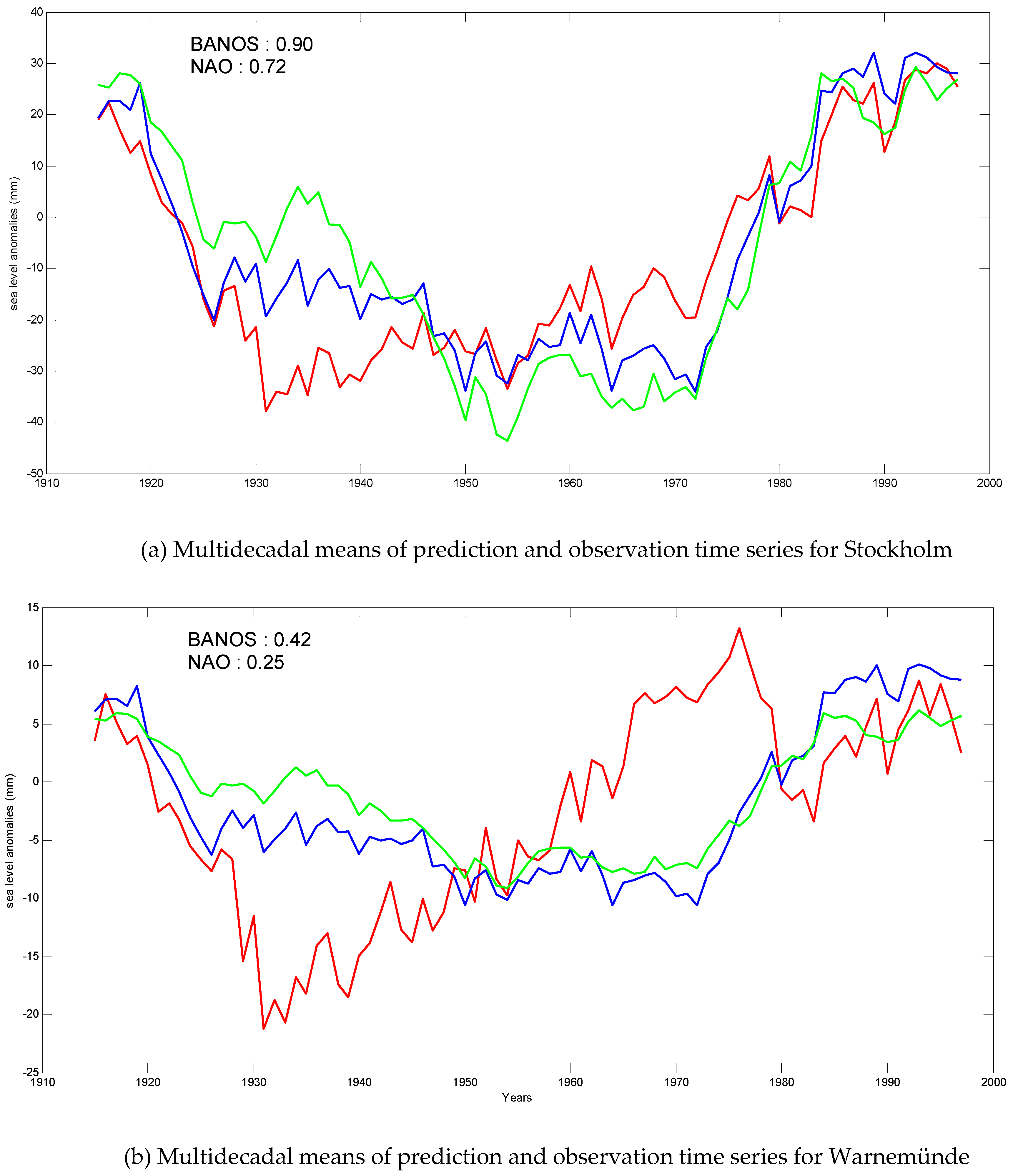
After quantifying the relation between the Baltic Sea level and the selected atmospheric indices through a linear regression, the contribution of the atmospheric circulation to the variations of Stockholm and Warnemünde sea level is predicted over the period 1900–2013. In the following step, the skill of linear regressions is measured by using the Brier Skill Score (BSS) values. The 31-year running means of predicted and observed sea levels are shown together with the corresponding BSS values in Figure 2.
Figure 2 shows the time evolution of predicted and observed sea level time series based on the 31-year time scale. On the one hand, a value of BSS zero means that the value of the mean (climatology) in the calibration period is the prediction value. On the other hand, negative BSS values indicate a worse skill than the simple climatological mean. This means that the best linear connection between atmosphere indices and the sea level variability in the Baltic Sea is captured by the connection between the BANOS index and the Stockholm tide gauge. The linear regression involving the relation between the NAO and the Warnemünde sea level has a skill slightly better than climatology, since the corresponding BSS value is slightly greater than zero (0.25).
4.3. Projections of the Atmosphere Indices and CorrespondingRanges of Sea Level Change
At this step, changes in the atmospheric indices are projected by using SLP outputs simulated by the CMIP5 climate models under the RCP8.5 scenario over the 21st century. The projections are computed from the difference of two normalized SLP fields. The geographical points of those SLP fields were described in the data set section. Projected variations of the BANOS and NAO indices are represented in Figure 3.
Figure 3 represents the projections of two atmospheric indices based on the SLP outputs of eight CMIP5 models driven by RCP8.5 forcings. For each climate model, three realizations were considered, each started from different initial conditions. The long-term trends of the indices in each simulation are computed by using linear regression. Trend estimations are shown in Table 4.
Table 4 shows that most of the models do not imply a significant trend at the 95% confidence level. Moreover, some realizations belonging to the same model resulted in atmospheric index trends of opposite sign.
Accordingly, the range of the Baltic Sea level rise that can be attributed to trends in atmospheric indices can be estimated for the end of 21st century. Using the sensitivity values of each tide gauge to the atmospheric indices, the highest BANOS-attributed Stockholm (Warnemünde) sea level rise is suggested as 11.7 cm (3.7 cm) by CCSM4. On the other hand, there are some estimations that indicate sea level sink due to the effect of these atmospheric circulation modes on the Stockholm and Warnemünde stations. One realization of the model MIROC5 implies a negative sea level trend due to the BANOS pattern effect. The amount of that negative trend suggests 3.1 cm (1.0 cm) Stockholm (Warnemünde) sea level fall due to the BANOS pattern untill the end of 21st century. However, none of those negative trends are significant.
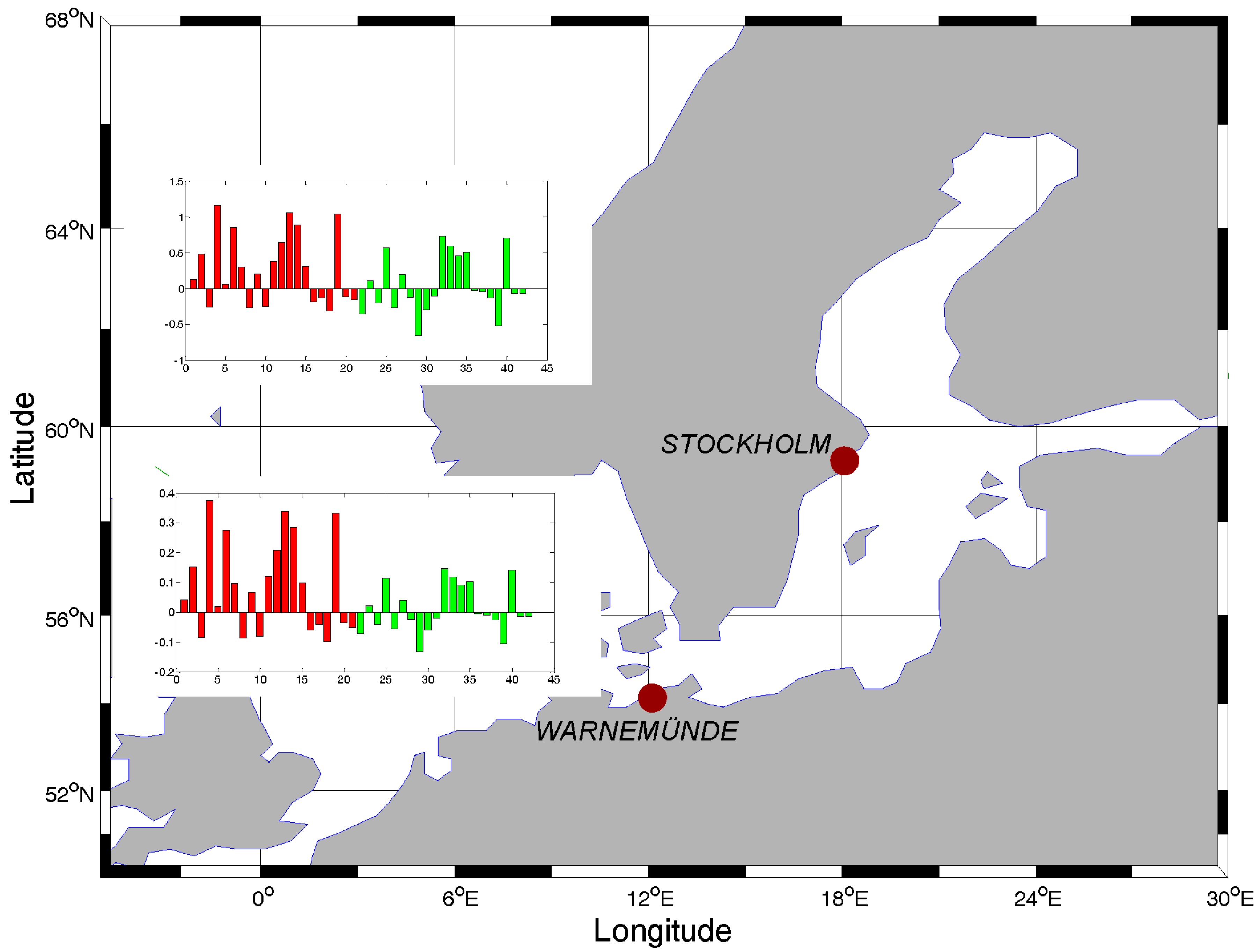
Considering the contribution of the NAO to the relative level-ends of Baltic Sea level changes, the model MPI-ESM-LR indicates highest-level end with the rate of 7.3 cm (1.5 cm) rise in Stockholm (Warnemünde). The lowest-level end is suggested by CanESM2 with the amount of 6.6 cm (1.3 cm) sink for the Stockholm (Warnemünde) station. The BANOS and NAO attributed sea-level trend estimations (mm/year), together with the locations of Stockholm and Warnemünde tide gauges are shown in Figure 4.
4.4. The Effect of Large-Scale Multidecadal Temperature Variability on Modes of Atmospheric Circulation
Finally, the possible effect of temperature on modes of atmospheric circulation, BANOS and NAO, is investigated for the period 1850–2100. The reason for this calculation is to ascertain whether the evolution of trend variations in the BANOS and NAO indices may be controlled by the large-scale SST trend variations, hence, the general rise of temperatures. Therefore, their trends could also be ascribed to anthropogenic radiative forcing. This statistical attribution would be derived from a correlation between the low-frequency variability of atmospheric indices and that of the mean temperature in the North Atlantic/European region.
For this investigation, correlations of 21-year window gliding trends between the spatially averaged temperature over the North Atlantic region and the BANOS index are considered. Correlation values consisting of 21-year gliding trends between the BANOS index and spatially averaged air temperature time series are shown in Table 5.
The correlation values are derived from three different realizations, with each of the CMIP5 models. As can be seen in Table 5, the correlations are close to zero and almost all of them are non-significant (r < 0.12) at the 95% significance level. In addition, some climate models indicate positive and negative correlation coefficients in different realizations. Results from the correlations of 21-year gliding trends between the NAO index and spatially averaged surface air temperature also did not indicate any connection (not shown). Overall, there is no long-term relation between the surface air temperature and the modes of atmospheric circulation.
5. Discussion
It can be argued that the method used in this study is limited, since the indices are constructed only by two special modes of atmospheric circulation. Therefore, they may not reflect the considerable influence of atmospheric circulation on the sea level trend in the Baltic Sea. This would be supported by the argument that other modes of the atmospheric variability can substantially influence sea level in the Baltic Sea over the 21st century. Relating to this argument, it should be noted that Hünicke [16] used several modes of atmospheric circulation in the European region in order to estimate the contribution of regional climate drivers to future winter sea level changes for the central and eastern Baltic Sea. That study applied a statistical downscaling approach to five different global climate model simulations driven by CMIP3 A2 scenario on decadal time scale. The main conclusion was that although there is a large spread of sea level rise estimations, the contribution of SLP to sea level changes indicates a positive trend in the central and eastern parts of the Baltic Sea.
There are two additional points that should be mentioned. The first one is that the simulated future trends in the NAO depend on the set of simulations analysed. The former ensemble of climate simulations belonging to the CMIP3 project indicates a clear intensification of the NAO under the A2 emission scenario, whereas the CMIP5 ensemble of simulations, driven by the RCP8.5 scenario, generally indicates weaker trends, also with a lower level of inter-mode agreement [21]. This means that if the present study had used the NAO index constructed from the output of the CMIP3, the results would likely be similar to those obtained by Hünicke [16]. The Intergovernmental Panel on Climate Change (IPCC) reported that there is an overall consistency between the CMIP3 and CMIP5 models for projecting both magnitudes of climate change and large-scale climate patterns. Differences in the outputs of CMIP3 and CMIP5 models exist mainly due to the change in climate scenarios [26,38].
The second and more crucial one is that the primary index used in this study was the BANOS index, which is a special index explaining the Baltic sea level variability strongly and steadily over time [15]. For instance, the BANOS index has a strong (significant) correlation to the Stockholm (Warnemünde) station with a value of 0.85 (0.55) in wintertime. However, the results of Hünicke and Zorita [8] illustrate that multivariate regression between leading components of the SLP fields covering the North Atlantic-West European sector and sea level imply a weak (insignificant) connection to the Stockholm-r = 0.48 (Warnemünde-r = 0.11) station in wintertime. It can be the case that the BANOS mode of the atmospheric circulation was not well captured in that study. Overall, this suggests that the BANOS index can be used to estimate the contribution of the large-scale atmospheric circulation to sea level rise in the Baltic Sea. It explains more variance of sea level than leading components of SLP fields (including NAO) in the North Atlantic-West European zone and connected steadily over time to sea level variation in the Baltic Sea.
This argument could also be further investigated by applying the same method as Hünicke [16] did to estimate the future sea level trends caused by changes in the atmospheric circulation, but by using the CMIP5 simulations instead of the CMIP3 simulations.
It should also be noted that Hünicke [16] detected a key role of precipitation in estimating the sea level change in the southern Baltic Sea, but the influence of BANOS pattern-related precipitation on sea level variability was found to be negligible for the whole of th eBaltic Sea in wintertime [15]. Superimposed on the BANOS index, the individual effects of the precipitation on future Baltic Sea level rise can also be investigated using CMIP5 precipitation outputs under the RCP8.5 scenario. However, a relational analysis like a multicollinearity test between the BANOS index and the precipitation field over the Baltic Sea basin should also be carried out prior to such an investigation in order to examine the possible significant dependency of those drivers [39].
Moreover, the results indicate that long-term effects are expected to dominate the Baltic Sea level trends over the 21st century. The most known long-term factor is vertical land motion due to the global isostatic adjustment (GIA) in the Baltic Sea in addition to global mean sea level rise (GMSL), due to anthropogenic forcing. It is previously mentioned that sea level trend projections of the RCP8.5 scenario indicate a GMSL rise in the range of between 0.52 and 0.98 m over the 21st century. However, the GIA effect has a spatially heterogeneous pattern over the Baltic Sea region (i.e., [40]). The largest vertical land motion rate attains 10 mm/year, which occurs close to the former centre of glaciations around the Gulf of Bothnia. Land subsidence is found in the southern part of the Baltic Sea with a rate of 1 mm/year, due to the crustal response of land along the edge of deglaciation area (i.e., [41]). For instance, GIA-induced vertical land motion causes 3.9 mm/year sea level to sink in Stockholm [42], and 0.3 mm/year sea level to rise in Warnemünde [40]. Considering these two long-term effects, relative sea level rise is likely to fluctuate in the range of 0.13 m (0.55 m) m and 0.59 m (1.01 m) in the Stockholm (Warnemünde) tide gauge under the RCP.85 scenario untill the end of 21st century. This estimation is valid in a case that sea level rise that may occur due to natural factors, which could not be included in the analysis of this study, remains small.
It is also worth nothing that this study is a statistical analysis aiming to establish a linear connection between atmospheric circulation modes and sea level variability. This sets a limitation on the analysis of sea level variability. Since the quantitative contribution of the driving factors to the sea level can only be estimated by numerical experiments with a realistic Baltic Sea ocean model. A numerical model could also provide information on non-linear interaction of those variables, which was not possible in this study.
It should also be clarified that the sea-level trend estimations of this study are based on two basic assumptions: that the statistical connection between sea-level and atmospheric indices remains unchanged over the 21st century, and that CMIP5 models are able to represent future projections well. For the future projection assumption, the CMIP5 models are tested in representing the present-day SLP climatology. The rationale behind this idea was that if the CMIP5 models fit the observations well, it is possible to estimate the future sea-level changes by relying on simulation outputs of those climate models.
6. Conclusions
This study investigates the influence of BANOS and NAO atmospheric circulation modes on future Baltic Sea level rise under the RCP8.5 scenario over the 21st century in wintertime. The main conclusions are:
- Most of the models simulate the SLP climatology reasonably well, although some models (HadGEM2-ES, CCSM4, CanESM2, MPI-ESM-LR, and FIO-ESM) show more realistic simulations in terms of the root-mean-square error and spatial correlation than the models MIROC5, IPSL-CM5A-LR and CSIRO-Mk3.6.0 models.
- Sea level variations in Stockholm and Warnemünde are better explained by the BANOS index than by the NAO index. In addition, a test on the skill of the statistical model shows that long-term sea level variability can be well represented by establishing a linear connection between the BANOS index and the Stockholm tide gauge. Concerning that relation, the Brier Skill Score (BSS) value indicates that an almost perfect prediction (BSS~0.90) is possible by using the linear relation between the BANOS index and the Stockholm sea level for the 31-year smoothed time series. Although this connection is sharply reduced in the southern Baltic, the BSS still indicates a considerable link reaching up to 0.42. These results also mean that BANOS plays a better role in capturing slow sea level variations than the NAO, since BSS results are affected by long-term differences of the mean value between the calibration and validation periods.
- Projected contributions of atmospheric circulation to sea level rise did not show a clear picture. More specifically, some models—even simulations within the same ensemble—displayed opposite trends. On the one hand, this implies that the influence of the internal climatic variability of CMIP5 models on the projected Baltic Sea level trends is large. On the other hand, it is likely that the contribution of atmospheric circulation modes to sea level rise in the Baltic Sea will remain relatively small through the 21st century.
- Correlations of 21-year window gliding trends between spatially averaged surface temperature over the North Atlantic and the BANOS index did not imply any long-term relation of multidecadal trends between the atmospheric condition and large-scale mean temperature for the period 1850–2100. This suggests the conclusion that the mode of atmospheric circulation that has a strong connection to the Baltic Sea level is not influenced by anthropogenic forcing in terms of the effect of air temperature, as in the case of the NAO.
Acknowledgments
The author thanks Eduardo Zorita and Birgit Hünicke for their help with this manuscript. The author is also grateful to Mark Carson for proofreading. This study was supported by the Deutsche Forschungsgemeinschaft (DFG) through the CliSAP project. The tide gauge data was obtained from the Permanent Service for Mean Sea Level, and some parts of the Stockholm data were courtesy of Martin Ekman. The author is grateful to NCAR for the meteorological and to NCEP/NCAR for the reanalysis data sets used in this study. The author also acknowledges the World Climate Research Programme’s Working Group on Coupled Modelling, which is responsible for CMIP, and the author thanks the climate modeling groups (listed in Table 1 of this study) for producing and making available their model output. For CMIP the U.S. Department of Energy’s Program for Climate Model Diagnosis and Intercomparison provides coordinating support and led development of software infrastructure in partnership with the Global Organization for Earth System Science Portals.
Conflicts of Interest
The author declares no conflict of interest.
References
- Church, J.A.; Clark, P.U.; Cazenave, A.; Gregory, J.M.; Jevrejeva, S.; Levermann, A.; Merrifield, M.A.; Milne, G.A.; Nerem, R.; Nunn, P.D.; et al. Sea level change. In Climate Change 2013: The Physical Science Basis. Contribution of Working Group I to the Fifth Assessment Report of the Intergovernmental Panel on Climate Change; Cambridge University Press: Cambridge, UK, 2013; pp. 1137–1216. [Google Scholar]
- Stammer, D.; Cazenave, A.; Ponte, R.M.; Tamisiea, M.E. Causes for contemporary regional sea level changes. Ann. Rev. Mar. Sci. 2013, 5, 21–46. [Google Scholar] [CrossRef] [PubMed]
- Slangen, A.B.; Carson, M.; Katsman, C.A.; van de Wal, R.S.W.; Köhl, A.; Vermeersen, L.L.A.; Stammer, D. Online Resource to: Projecting twenty-first century regional sea-level changes. Clim. Chang. 2014, 124, 317–332. [Google Scholar] [CrossRef]
- Carson, M.; Köhl, A.; Stammer, D.; Slangen, A.A.B.; Katsman, C.A.; van de Wal, R.S.W.; Church, J.; White, N. Coastal sea level changes, observed and projected during the 20th and 21st century. Clim. Chang. 2016, 134, 269–281. [Google Scholar] [CrossRef]
- Grinsted, A.; Jevrejeva, S.; Riva, R.E.M.; Dahl-Jensen, D. Sea level rise projections for northern Europe under RCP8. Clim. Res. 2015, 64, 15–23. [Google Scholar] [CrossRef]
- Yan, Z.; Tsimplis, M.N.; Woolf, D. Analysis of the relationship between the North Atlantic oscillation and sea-level changes in northwest Europe. Int. J. Climatol. 2004, 24, 743–758. [Google Scholar] [CrossRef]
- Jevrejeva, S.; Moore, J.C.; Woodworth, P.L.; Grinsted, A. Influence of large-scale atmospheric circulation on European sea level: Results based on the wavelet transform method. Tellus A 2005, 57, 183–193. [Google Scholar] [CrossRef]
- Hünicke, B.; Zorita, E. Influence of temperature and precipitation on decadal Baltic Sea level variations in the 20th century. Tellus A 2006, 58, 141–153. [Google Scholar] [CrossRef]
- Moeller, J.S.; Hansen, I.S. Hydrographic processes and changes in the Baltic Sea. Dana 1994, 10, 87–104. [Google Scholar]
- Leppäranta, M.; Myrberg, K. Physical Oceanography of the Baltic Sea; Springer: Berlin/Heidelberg, Germany; New York, NY, USA, 2009. [Google Scholar]
- Hünicke, B.; Zorita, E.; Soomere, T.; Madsen, K.S.; Johansson, M.; Suursaar, Ü. Recent change—Sea level and wind waves. In Second Assessment of Climate Change for the Baltic Sea Basin; Springer: Cham, Germany; Heidelberg, Germany; New York, NY, USA; Dordrecht, The Netherlands; London, UK, 2015; pp. 155–185. [Google Scholar]
- Andersson, H.C. Influence of long-term regional and large-scale atmospheric circulation on the Baltic sea level. Tellus A 2002, 54, 76–88. [Google Scholar] [CrossRef]
- Heyen, H.; Zorita, E.; von Storch, H. Statistical downscaling of monthly mean North Atlantic air-pressure to sea level anomalies in the Baltic Sea. Tellus A 1996, 48, 312–323. [Google Scholar] [CrossRef]
- Hünicke, B.; Luterbacher, J.; Pauling, A.; Zorita, E. Regional differences in winter sea level variations in the Baltic Sea for the past 200 year. Tellus A 2008, 60, 384–393. [Google Scholar] [CrossRef]
- Karabil, S.; Zorita, E.; Hünicke, B. Contribution of atmospheric circulation to recent off-shore sea-level variations in the Baltic Sea and the North Sea. Earth Syst. Dyn. Discuss. 2017. [Google Scholar] [CrossRef]
- Hünicke, B. Contribution of regional climate drivers to future winter sea-level changes in the Baltic Sea estimated by statistical methods and simulations of climate models. Int. J. Earth Sci. 2010, 99, 1721–1730. [Google Scholar] [CrossRef]
- Johansson, M.M.; Pellikka, H.; Kahma, K.K.; Ruosteenoja, K. Global sea level rise scenarios adapted to the Finnish coast. J. Mar. Syst. 2014, 129, 35–46. [Google Scholar] [CrossRef]
- Czaja, A.; Robertson, A.W.; Huck, T. The Role of Atlantic Ocean-Atmosphere Coupling in Affecting North Atlantic Oscillation Variability. In The North Atlantic Oscillation: Climatic Significance and Environmental Impact; American Geophysical Union: Washington, DC, USA, 2003; pp. 147–172. [Google Scholar]
- Rodwell, M.J.; Rowell, D.P.; Folland, C.K. Oceanic forcing of the wintertime North Atlantic Oscillation and European climate. Nature 1999, 398, 320–323. [Google Scholar] [CrossRef]
- Greatbatch, R.J. The North Atlantic Oscillation. Stoch. Environ. Res. Risk Assess. 2000, 14, 213–242. [Google Scholar] [CrossRef]
- Cattiaux, J.; Cassou, C. Opposite CMIP3/CMIP5 trends in the wintertime Northern Annular Mode explained by combined local sea ice and remote tropical influences. Geophys. Res. Lett. 2013, 40, 3682–3687. [Google Scholar] [CrossRef]
- BACC II Author Team (Ed.) Second Assessment of Climate Change for the Baltic Sea Basin; Springer: Cham, Germany; Heidelberg, Germany; New York, NY, USA; Dordrecht, The Netherlands; London, UK, 2015. [Google Scholar]
- Novotny, K.; Liebsch, G.; Lehmann, A.; Dietrich, R. Variability of Sea Surface Heights in the Baltic Sea: An Intercomparison of Observations and Model Simulations. Mar. Geod. 2006, 29, 113–134. [Google Scholar] [CrossRef]
- Holgate, S.J.; Matthews, A.; Woodworth, P.L.; Rickards, L.J.; Tamisiea, M.E.; Bradshaw, E.; Foden, P.R.; Gordon, K.M.; Jevrejeva, S.; Pugh, J. New Data Systems and Products at the Permanent Service for Mean Sea Level. J. Coast. Res. 2013, 29, 493–504. [Google Scholar] [CrossRef]
- Ekman, M. The World’s Longest Sea Level Series and a Winter Oscillation Index for Northern Europe 1774–2000; Small Publications in Historical Geophysics; Summer Institute for Historical Geophysics: Åland Islands, Finland, 2003; Volume 12, p. 32. [Google Scholar]
- Taylor, K.E.; Stouffer, R.J.; Meehl, G.A. An overview of CMIP5 and the experiment design. Bull. Am. Meteorol. Soc. 2012, 93, 485–498. [Google Scholar] [CrossRef]
- Kalnay, E.; Kanamitsu, M.; Kistler, R.; Collins, W.; Deaven, D.; Gandin, L.; Iredell, M.; Saha, S.; White, G.; Woollen, J.; et al. The NCEP/NCAR 40-year reanalysis project. Bull. Am. Meteorol. Soc. 1996, 77, 437–471. [Google Scholar] [CrossRef]
- Riahi, K.; Gruebler, A.; Nakicenovic, N. Scenarios of long-term socio-economic and environmental development under climate stabilization. Technol. Forecast. Soc. Chang. 2007, 74, 887–935. [Google Scholar] [CrossRef]
- Riahi, K.; Rao, S.; Krey, V.; Cho, C.; Chirkov, V.; Fischer, G.; Kindermann, G.; Nakicenovic, N.; Rafaj, P. RCP 8.5-A scenario of comparatively high greenhouse gas emissions. Clim. Chang. 2011, 109, 33–57. [Google Scholar] [CrossRef]
- Hurrell, J.W.; National Center for Atmospheric Research Staff. Last modified 06 April 2016. The Climate Data Guide: NCAR Sea Level Pressure. Available online: https://climatedataguide.ucar.edu/climate-data/ncar-sea-level-pressure (accessed on 10 May 2016).
- Hurrell, J.W.; National Center for Atmospheric Research Staff (Eds.) Last Modified 2 March 2016. The Climate Data Guide: Hurrell North Atlantic Oscillation (NAO) Index (Station-Based). Available online: https://climatedataguide.ucar.edu/climate-data/hurrell-north-atlantic-oscillation-nao-index-station-based (accessed on 2 March 2016).
- Hurrell, J.W.; Kushnir, Y.; Otterson, G.; Visbeck, M. An Overview of the North Atlantic Oscillation. In The North Atlantic Oscillation: Climatic Significance and Environmental Impact; American Geophysical Union: Washington, DC, USA, 2003; Volume 134, p. 263. [Google Scholar] [CrossRef]
- Taylor, K.E. Summarizing multiple aspects of model performance in a single diagram. J. Geophys. Res. 2001, 106, 7183–7192. [Google Scholar] [CrossRef]
- Wakelin, S.L.; Woodworth, P.L.; Flather, R.A.; Williams, J.A. Sea-level dependence on the NAO over the NW European Continental Shelf. Geophys. Res. Lett. 2003, 30. [Google Scholar] [CrossRef]
- Von Storch, H.; Zwiers, F.W. Statistical Analysis in Climate Research. J. Am. Stat. Assoc. 1999, 95, 1375. [Google Scholar] [CrossRef]
- Fenech, A.; Comer, N.; Gough, B. Selecting a global climate model for understanding future projections of climate change. In Linking Climate Models to Policy and Decision-Making; UPEI Climate Lab, Prince Edward Island: Toronto, ON, Canada, 2002; pp. 133–145. [Google Scholar]
- Flato, G.; Marotzke, J.; Abiodun, B.; Braconnot, P.; Chou, S.C.; Collins, W.J.; Forest, C.P.; Gleckler, E.; Guilyardi, C.; Jakob, V.; et al. Evaluation of Climate Models. In Climate Change 2013: The Physical Science Basis. Contribution of Working Group I to the Fifth Assessment Report of the Intergovernmental Panel on Climate Change; Stocker, T.F., Qin, D., Plattner, G.-K., Tignor, M.M.B., Allen, S.K., Boschung, J., Nauels, A., Xia, Y., Bex, V., Midgley, P.M., Eds.; Cambridge University Press: Cambridge, UK, 2013; pp. 741–866. [Google Scholar]
- Intergovernmental Panel on Climate Change (IPCC). Climate Change 2013: The Physical Science Basis. Contribution of Working Group I to the Fifth Assessment Report of the Intergovernmental Panel on Climate Change; Stocker, T.F., Qin, D., Plattner, G.-K., Tignor, M.M.B., Boschung, J., Nauels, A., Xia, Y., Bex, V., Midgley, P.M., Eds.; Cambridge University Press: Cambridge, UK, 2013. [Google Scholar]
- Sterlini, P.; Vries, H.; Katsman, C. Sea surface height variability in the North East Atlantic from satellite altimetry. Clim. Dyn. 2016, 47, 1285–1302. [Google Scholar] [CrossRef]
- Richter, A.; Groh, A.; Dietrich, R. Geodetic observation of sea-level change and crustal deformation in the Baltic Sea region. Phys. Chem. Earth 2011, 53, 43–53. [Google Scholar] [CrossRef]
- Lidberg, M.; Johansson, J.M.; Scherneck, H.G.; Milne, G.A. Recent results based on continuous GPS observations of the GIA process in Fennoscandia from BIFROST. J. Geodyn. 2010, 50, 8–18. [Google Scholar] [CrossRef]
- Peltier, W.R. Global Glacial Isostasy and the Surface of the Ice-age Earth: The ICE-5G (VM2) Model and GRACE. Annu. Rev. Earth Planet. Sci. 2004, 32, 111–149. [Google Scholar] [CrossRef]
Figure 1.
Taylor Diagram displaying the statistical comparison of 30-year SLP means considering the relative differences of eight CMIP5 models ((1) MOHC: HadGEM2ES; (2) NCAR: CCSM4; (3) CCCMA: CanESM2; (4) MPI-M: MPI-ESM-LR; (5) FIO: FIO-ESM; (6) MIROC: MIROC5; (7) IPSL: IPSL-CM5A-LR; (8) CSIRO-QCCCE: CSIRO-Mk3.6.0) with respect to SLP reanalysis values (REF). Models are ranked and numbered based on their relative performances. The SLP means were selected over the geographical area covering the Baltic Sea and the North Sea. The green arcs represent root mean square differences (RMSD), black arcs show standard deviation values and blue lines indicate correlation values.

Figure 2.
The 31-year running means of predicted (blue: the Baltic Sea and North Sea Oscillation (BANOS) index predicted; green: the NAO index predicted) and observed (red) sea levels of the Stockholm and Warnemünde stations (top panel is for Stockholm) together with the BSS values in the 31-year mean smoothed time series. Note the different y-axis scales. The numbers in the figure indicate the BSS values.

Figure 3.
Projections of the atmospheric indices (BANOS and NAO) variations. The CMIP5 models on the top panel show the BANOS index projections, the CMIP5 models on the bottom panel show the NAO index projections. The models are ranked from top (best) to bottom (worst) with respect to their performances. The lines represent ensemble means and the shaded areas show individual ensemble spreads.

Figure 4.
The Baltic Sea region map including the locations of Stockholm and Warnemünde tide gauges. The bar graphs show the atmospheric index driven trend estimations of the sea-level (mm/year). The panel at the top (bottom) shows the BANOS-red and NAO-green driven sea-level trends in Stockholm (Warnemünde). The estimations are ordered based on the performance of the CMIP5 models. For instance, the first three estimations are deduced from realizations of the model HadGEM2-ES for each index.


Table 1.
The list of the selected CMIP5 models with individual grid resolution. At this stage, the models are ranked based on the alphabetical order. The Institute IDs stand for CCCMA: Canadian Centre for Climate Modelling and Analysis, NCAR: National Center for Atmospheric Research, CSIRO-QCCCE: Commonwealth Scientific and Industrial Research Organization in collaboration with Queensland Climate Change Centre of Excellence, FIO: The First Institute of Oceanography, MOHC: Met Office Hadley Centre, IPSL: Institut Pierre-Simon Laplace, MIROC: Atmosphere and Ocean Research Institute (The University of Tokyo), National Institute for Environmental Studies, and Japan Agency for Marine-Earth Science and Technology, MPI-M: Max Planck Institute for Meteorology.
| Model Name | Institute ID | Atmospheric Grid | |
|---|---|---|---|
| Latitude | Longitude | ||
| CanESM2 | CCCMA | 2.7906 | 2.8125 |
| CCSM4 | NCAR | 0.9424 | 1.2500 |
| CSIRO-Mk3.6.0 | CSIRO-QCCCE | 1.8653 | 1.8750 |
| FIO-ESM | FIO | 2.7906 | 2.8125 |
| HadGEM2-ES | MOHC | 1.2500 | 1.8750 |
| IPSL-CM5A-LR | IPSL | 1.8947 | 3.7500 |
| MIROC5 | MIROC | 1.4008 | 1.4063 |
| MPI-ESM-LR | MPI-M | 1.8653 | 1.8750 |
Table 2.
Correlation coefficients between atmospheric indices and tide gauges are represented for the period 1900–2013 in wintertime. Notably, time series are detrended prior to the correlation computation. * The correlation between the North Atlantic Oscillation (NAO) index and the Warnemünde station is insignificant at the two-sided 95% confidence level.
| Correlation | ||
|---|---|---|
| Index/Station | Stockholm | Warnemünde |
| BANOS | 0.85 | 0.55 |
| NAO | 0.55 | 0.17 * |
Table 3.
The sensitivity values of sea level are estimated per one unit change in the associated index. For the estimation, a linear regression is implemented where sea level is the predictand and atmospheric index is the predictor. Time series are detrended prior to the sensitivity computation.
Table 3.
The sensitivity values of sea level are estimated per one unit change in the associated index. For the estimation, a linear regression is implemented where sea level is the predictand and atmospheric index is the predictor. Time series are detrended prior to the sensitivity computation.
| Sensitivity of Stations (mm/u) | ||
|---|---|---|
| Index/Station | Stockholm | Warnemünde |
| BANOS | 73 | 23 |
| NAO | 54 | 11 |
Table 4.
Trends of the BANOS and NAO indices with their associated standard errors over the period 2006–2100. The significant trends at the 95% confidence level are marked (*). The letter ‘u’ stands for the word ‘Index Unit’. Last two columns at the right side refer to the sea-level trends in Stockholm due to trends in the corresponding atmospheric indices. For the associated trend of Warnemünde, sea-level trend estimations (mm/year) in the BANOS (NAO) column should be multiplied with the factor 0.32 (0.20).
| Model | Realization | Trend ± 1 SE (u/year) xe² | Trend ± 1 SE (mm/year) | ||
|---|---|---|---|---|---|
| BANOS | NAO | BANOS | NAO | ||
| HadGEM2-ES | r1i1p1 | 0.18 ± 0.55 | −0.67 ± 0.56 | 0.13 ± 0.40 | −0.36 ± 0.30 |
| r2i1p1 | 0.65 ± 0.51 | 0.20 ± 0.58 | 0.48 ± 0.38 | 0.11 ± 0.31 | |
| r3i1p1 | −0.36 ± 0.52 | −0.38 ± 0.57 | −0.26 ± 0.38 | −0.20 ± 0.31 | |
| CCSM4 | r1i1p1 | 1.60 ± 0.55 * | 1.05 ± 0.54 | 1.17 ± 0.40 * | 0.57 ± 0.29 |
| r2i1p1 | 0.08 ± 0.55 | −0.49 ± 0.52 | 0.06 ± 0.40 | −0.27 ± 0.28 | |
| r3i1p1 | 1.17 ± 0.51 * | 0.36 ± 0.54 | 0.86 ± 0.38 * | 0.20 ± 0.29 | |
| CanESM2 | r1i1p1 | 0.42 ± 0.58 | −0.22 ± 0.58 | 0.30 ± 0.42 | −0.12 ± 0.32 |
| r2i1p1 | −0.37 ± 0.57 | −1.22 ± 0.53 * | −0.27 ± 0.41 | −0.66 ± 0.29 * | |
| r3i1p1 | 0.29 ± 0.57 | −0.54 ± 0.56 | 0.21 ± 0.42 | −0.29 ± 0.30 | |
| MPI-ESM-LR | r1i1p1 | −0.35 ± 0.56 | −0.18 ± 0.56 | −0.25 ± 0.41 | −0.10 ± 0.30 |
| r2i1p1 | 0.52 ± 0.52 | 1.35 ± 0.54 * | 0.38 ± 0.38 | 0.73 ± 0.29 * | |
| r3i1p1 | 0.89 ± 0.53 | 1.09 ± 0.56 | 0.65 ± 0.38 | 0.59 ± 0.30 | |
| FIO-ESM | r1i1p1 | 1.45 ± 0.50 * | 0.86 ± 0.49 | 1.06 ± 0.37 * | 0.46 ± 0.26 |
| r2i1p1 | 1.22 ± 0.52 * | 0.93 ± 0.51 | 0.89 ± 0.38 * | 0.51 ± 0.28 | |
| r3i1p1 | 0.42 ± 0.53 | −0.05 ± 0.53 | 0.31 ± 0.39 | −0.03 ± 0.29 | |
| MIROC5 | r1i1p1 | −0.24 ± 0.55 | −0.08 ± 0.53 | −0.18 ± 0.40 | −0.05 ± 0.29 |
| r2i1p1 | −0.18 ± 0.55 | −0.25 ± 0.57 | −0.13 ± 0.40 | −0.13 ± 0.31 | |
| r3i1p1 | −0.43 ± 0.51 | −0.97 ± 0.54 | −0.31 ± 0.37 | −0.52 ± 0.29 | |
| IPSL-CM5A-LR | r1i1p1 | 1.42 ± 0.50 * | 1.32 ± 0.50 * | 1.04 ± 0.37 * | 0.71 ± 0.27 * |
| r2i1p1 | −0.15 ± 0.50 | −0.13 ± 0.52 | −0.11 ± 0.37 | −0.07 ± 0.28 | |
| r3i1p1 | −0.22 ± 0.54 | −0.13 ± 0.55 | −0.16 ± 0.40 | −0.07 ± 0.30 | |
Table 5.
Correlations of 21-year gliding trends between spatial mean of surface air temperature and the BANOS index are shown for the period 1850–2100. The value of two-sided 95% significance level is 0.12 for this record length. The significant correlation coefficients are marked (*).
Table 5.
Correlations of 21-year gliding trends between spatial mean of surface air temperature and the BANOS index are shown for the period 1850–2100. The value of two-sided 95% significance level is 0.12 for this record length. The significant correlation coefficients are marked (*).
| Model | Correlations of 21-Year Gliding Trends | ||
|---|---|---|---|
| r1i1p1 | r2i1p1 | r3i1p1 | |
| HadGEM2-ES | −0.12 | 0.18 * | 0.04 |
| CCSM4 | −0.14 * | −0.07 | −0.08 |
| CanESM2 | 0.05 | −0.12 | −0.16 * |
| MPI-ESM-LR | 0.13 * | −0.05 | −0.07 |
| FIO-ESM | 0.01 | −0.09 | −0.03 |
| MIROC5 | −0.25 * | −0.26 * | −0.24 * |
| IPSL-CM5A-LR | 0.12 | −0.03 | 0.10 |
| CSIRO-Mk3.6.0 | −0.05 | 0.20 * | 0.30 * |
© 2017 by the author. Licensee MDPI, Basel, Switzerland. This article is an open access article distributed under the terms and conditions of the Creative Commons Attribution (CC BY) license (http://creativecommons.org/licenses/by/4.0/).
Share and Cite
MDPI and ACS Style
Karabil, S. Influence of Atmospheric Circulation on the Baltic Sea Level Rise under the RCP8.5 Scenario over the 21st Century. Climate 2017, 5, 71. https://0-doi-org.brum.beds.ac.uk/10.3390/cli5030071
AMA Style
Karabil S. Influence of Atmospheric Circulation on the Baltic Sea Level Rise under the RCP8.5 Scenario over the 21st Century. Climate. 2017; 5(3):71. https://0-doi-org.brum.beds.ac.uk/10.3390/cli5030071
Chicago/Turabian StyleKarabil, Sitar. 2017. "Influence of Atmospheric Circulation on the Baltic Sea Level Rise under the RCP8.5 Scenario over the 21st Century" Climate 5, no. 3: 71. https://0-doi-org.brum.beds.ac.uk/10.3390/cli5030071
Note that from the first issue of 2016, this journal uses article numbers instead of page numbers. See further details here.