Article

Modelling Hydrological Components of the Rio Maipo of Chile, and Their Prospective Evolution under Climate Change

by
Daniele Bocchiola
1,2,*,
Andrea Soncini
1,
Antonella Senese
3 and
Guglielmina Diolaiuti
3
1
Department of Civil and Environmental Engineering (DICA-SIA), Politecnico di Milano, 20133 Milano, Italy
2
EVK2CNR Association, San Bernardino 145, 24126 Bergamo, Italy
3
Department of Environmental Scientce and Policies, Università di Milano, Celoria 2, 20133 Milano, Italy
*
Author to whom correspondence should be addressed.
Submission received: 17 May 2018 / Revised: 7 June 2018 / Accepted: 20 June 2018 / Published: 25 June 2018
(This article belongs to the Special Issue Modified Hydrological Cycle under Global Warming)

Abstract

:
We used the Poly-Hydro model to assess the main hydrological components of the snow-ice melt driven Maipo River in Chile, and glaciers’ retreat under climate change therein until 2100. We used field data of ice ablation, ice thickness, weather and hydrological data, and precipitation from TRMM. Snow cover and temperature were taken from MODIS. We forced the model using weather projections until 2100 from three GCMs from the IPCC AR5, under three different radiative concentration pathways (RCPs 2.6, 4.5, 8.5). We investigated trends of precipitation, temperature, and hydrology until 2100 in the projection period (PR, 2014–2100) and the whole period (CM 1980–2100, composite), against historical trends in control period (CP, 1980–2013). We found potentially increasing temperature until 2100, except for Spring (OND). In the PR period, yearly flow decreases significantly under RCP85, on average −0.25 m3·s−1·year−1, and down to −0.48 m3·s−1·year−1, i.e., −0.4% year−1 against CP yearly average (120 m3 s−1). In the long run (CM) significant flow decrease would, occur under almost all scenarios, confirming persistence of a historical decrease, down to −0.39 m3·s−1·year−1 during CM. Large flow decreases are expected under all scenarios in Summer (JFM) during PR, down to −1.6 m3·s−1·year−1, or −1% year−1 against CP for RCP8.5, due to increase of evapotranspiration in response to higher temperatures. Fall (AMJ) flows would be mostly unchanged, while Winter (JAS) flows would be projected to increase significantly, up to 0.7 m3·s−1·year−1 during 2014–2100, i.e., +0.9% year−1 vs. CP under RCP8.5, due to large melting therein. Spring (OND) flows would decrease largely under RCP8.5, down to −0.67 m3 s−1·year−1, or −0.4% year−1 vs. CP, again due to evapotranspiration. Glacier down wasting is projected to speed up, and increasingly so with RCPs. Until 2100 ice loss would range from −13% to −49% (−9%, and −39% at 2050) of the estimated volume at 2012, which changed by −24% to −56% (−21%, and −39% at 2050) vs. ice volume in 1982, thus with rapider depletion in the first half of the century. Policy makers will have to cope with modified hydrological cycle in the Maipo River, and greatly decreasing ice cover in the area.

1. Introduction

Water security in the Andean region is at stake under demographic pressure, the changing climate, and glaciers’ shrinking under climate change lately [1,2,3,4,5,6]. Central Chile is semi-arid with mostly dry Summer, and rain in Winter, and snow and glaciers’ melt contributes runoff in the Summer up to 70–80%. Since the 70s, ~50% of Andean cryosphere wasted under a +0.7 °C increase [7,8], with an initial increase in discharge, but likely a decrease in the long run, also in response to decrease of snowfall [9,10,11]. Santiago region (with 7 M+ inhabitants) takes most (70–90%) agricultural water from the Maipo River [12], with water use expected to increase along the century [13].
Among others recently, Pellicciotti et al. [6] reviewed recent status of glaciers of Chile. They found glaciers shrinking rapidly in the central Andes, i.e., the Juncal Norte, Juncal Sur, and Olivares Gamma glaciers, the two latter dwelling in the Maipo catchment, wasting to −2.4%, −10.9%, and −8.2% in area since 1955 [1]. Our study here aims at setting up a hydrological model to sketch the present and future hydrological regime, and hydrological components of the basin of Rio Maipo Alto, a high altitude area, where gathering of information is complex given harsh environmental conditions [14,15,16,17]. To make up for the sparseness of data at the highest altitudes, we used series of precipitation from the Tropical Rainfall Measurement Mission (TRMM), and temperature from the Moderate Resolution Imaging Spectroradiometer (MODIS). The manuscript structure is as follows. (i) In Section 2 we describe the case study area, data base, the climate projections from the chosen general circulation models GCMs; (ii) in Section 3 we describe hydro-glaciological modelling, projections until 2100, and assessment of future meteo-hydrological trends; (iii) in Section 4 we report the main results of our exercise; (iv) in Section 5 we provide discussion, and benchmarking against recent findings; and (v) in Section 6 we report our conclusions, and outlooks.
The work partly builds on a former study [18] focusing upon the Maipo River. Here we provided much wider insight, namely by (i) projecting future hydrology under two more GCMs, so exploring a wider range of climate uncertainty; (ii) explicitly investigating past, and future trends of glaciers’ cover; (iii) explicitly investigating the importance, and potential future evolution of flow components; (iv) explicitly investigating past, and potential future flow trends under the defined variability range; and (v) performing a correlation analysis between in stream flows and climate drivers, for the historical and projected data, to assess changes between present and future flow generating mechanisms, and the climate. Accordingly, our results here are original and of large interest for scientists, and policy makers in the Andean region.

2. Case Study and Data Base
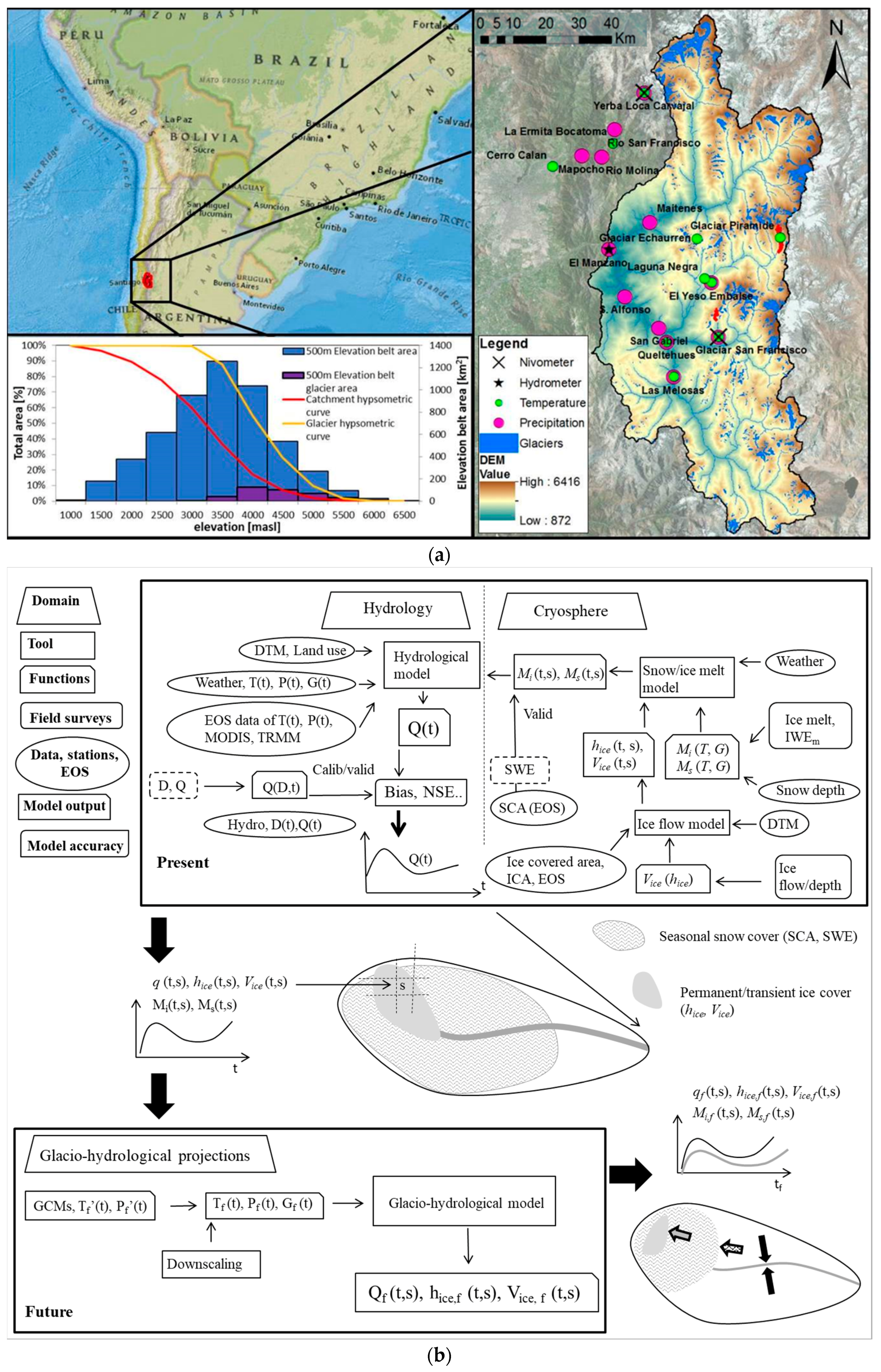
2.1. Maipo River

The case study area was the basin of Maipo River (Central Chile), closed at El Manzano (a small town along the river, ca. 15 km upstream Santiago, 890 m a.s.l., 4839 km2, in Figure 1), nesting the upper Maipo, and its main tributaries (Olivares, Colorado, Yeso and Volcàn). The catchment covered 33°4′ S to 34°15′ S, and altitude varied between 890 m a.s.l. to more than 6500 m a.s.l. of Tupungato. About 90% of the area was above 2000 m a.s.l., and 60% above 3000 m a.s.l. There was 364 km2 of glaciers, i.e., 8% of the area. Average flow was 120 m3 s−1 (1980–2013).
Soil was bare (54%), with bushes (24%), snowfields and glaciers (8%), and elsewhere forest, prairie, and steppe (MODIS, MCD12Q1, 500 m resolution). At the lowest altitudes the climate was temperate Mediterranean, with dry Summer and wet Winter (May to August, 95% of annual precipitation). Summers were hot with 30 °C+, and strong thermal excursion and cold climate at high altitudes (above 2500 m a.s.l) were seen. Winter temperature was largely below 0 °C and considerable snow falls occur [19]. Rainfall increased from North to South [20]. Two main reservoirs were present in the catchment, i.e., Laguna Negra (600 Mm3) and el Yeso (250 Mm3, on the Rio Yeso River).

2.2. Historical Weather and Hydro Data

Poly-Hydro model needs daily temperature and precipitation. The grid size adopted here was 3 × 3 km2, somewhat large given the size of glaciers within the catchment (the largest being Juncal Sur, ca. 21 km2). However, given the size of Maipo catchment, such grid size was a reasonable trade-off between description distributed processes including ice flow, and computational burden for long term simulation of climate change scenarios. Accordingly, input data of precipitation, and temperature were distributed over a 3 × 3 km2 grid, and fed to the model. To aid proper spatial interpolation on the model grid, and to capture local patterns in temperature, and precipitation, we complemented the information from ground stations with data from TRMM, and MODIS satellites, reported below in Section 3. In Figure 1b a flow chart is reported, resuming the modelling approach and components, data requirements, tuning methods, and water resources projections under climate change (see also [17] for reference).
We used data from ten temperature stations, seven in the Maipo basin Rio Alto, and three northeast of Santiago (Rio Mapocho, Figure 1, Table 1). There were 11 rainfall stations available (Figure 1, Table 1) below snow line. Data from the station Yerba Loca Carvajal could not be used because the station was not heated, and snow water equivalent was not accounted for systematically. The stations were property of the Direcciòn General de Aguas DGA (except for one on the Pyramid glacier, property of EvK2CNR), and three were higher than 3000 m a.s.l. Monthly temperature lapse rates were estimated from stations with at least eight years of data, and varied from −6.9 °C km−1, to of −5.2 °C km−1, in February and December. Precipitation increases with altitude, from +3 mm km−1 in December (Spring) to +200 mm km−1 in July (Winter). The DGA made available daily flows (m3 s−1) at El Manzano (Figure 1). In the Maipo catchment one snow depth station was present near the San Francisco glacier at 2220 m a.s.l. (Figure 1), and we could also use the Yerba Loca Carvajal snow station, close to the divide (3250 m a.s.l.).

2.3. Satellite Data

We used temperature data from MOD11C3 product of MODIS (Moderate Resolution Imaging Spectroradiometer) on board of Terra (EOS AM), during 2002–2012. Rainfall distribution in space was assessed using data from TRMM (Tropical Rainfall Measuring Mission, TRMM 2B31, [21,22]) during 1998–2009 (4 × 4 km2), obtained by fusion of Precipitation Radar (PR) data, and TRMM Microwave Imager data [23]. Simulated snow coverage (i.e., water equivalent SWE) was validated against MOD10A2 product at 500 m resolution (snow covered area), 8 days composite [24,25,26] during 2010–2012.

2.4. Field Campaigns

Field data were gathered in 2012 by personnel of EvK2CNR in the project “Action plan for the safeguarding of the glaciers against climate change” of DGA, including measurements on San Francisco, and Pyramid glaciers [18]. San Francisco glacier had seven ablation stakes, at 2890–3425 m a.s.l. Pyramid is a debris covered glacier, and supraglacial rock debris strongly affects ice melt [27], so we assessed melt factors against debris thickness [15,16,28].

2.5. Climate Projections

The Fifth Assessment Report (AR5) by the Intergovernmental Panel on Climate Change IPCC presented scenarios describing four different Representative Concentration Pathways (RCPs, 2.6, 4.5, 6.5, 8.5 [29]). Temperature and precipitation were taken according to RCP2.6 (peak in radiative forcing at 3 Wm−2 or 490 ppm CO2 equivalent at 2040, with decline to 2.6 Wm−2), RCP4.5 (stabilization without overshoot pathway to 4.5 Wm−2, or 650 ppm CO2 eq. at 2070), and RCP8.5 (rising radiative forcing up to 8.5 Wm−2, or 1370 ppm CO2 eq. by 2100). Three GCM models were used for this study (Table 2), i.e., CCSM4 ([30], https://www.earthsystemgrid.org), EC-Earth ([31], http://ecearth.knmi.nl/) and ECHAM6 ([32], http://cera-www.dkrz.de). The low spatial resolution of GCMs requires downscaling to perform hydrological/impact studies at the basin scale [33].

3. Methods

3.1. Glacio-Hydrological Modelling

Poly-Hydro model [17,34] was used here, developed at Politecnico di Milano. The Poly-Hydro model can be used to mimic hydrology of high altitude catchments [15,26,35,36]. We do not report here all model’s equations, and the reader is referred to the literature above. Glacier flow is modeled as driven by gravity [15]. Ice flow velocity is depicted by a simplified force balance, proportional to shear stress to a power n, i.e., with Glen´s flow law (n = 3, e.g., [37,38]). Basal shear stress τb (Pa) is either known or estimated, and accounting for deformation and sliding velocity as governed by τb one can approximate depth averaged ice velocity as [39]:
V i c e , i = K d τ b , i n h i c e , i + K s τ b , i n h i c e , i ,
with hice,i (m) ice thickness in the cell i, and Ks (m−3·year−1) and Kd (m−1·year−1) parameters of basal sliding and internal deformation. Model tuning was carried out using observed flow velocities for the San Francisco, and Pyramid glaciers, where ice thickness was known via GPR measurements [40]. Initialization was pursued by estimating ice thickness hice,i for each cell (with ice cover) within our catchment, to subsequently estimate basal shear τb as:
τ b , i = ρ i g h i c e , i sin α i ,
with ρi ice density (kg m−3), g gravity (9.8 m s−2), and αi slope. DGA provided estimated ice thickness at 2012 for all glaciers of the Maipo catchments. Avalanching on the glaciers is accounted for by considering the terrain slope (linearly increasing within 30°–60°, [34]). The cell size used here was 3 × 3 km2 as reported, giving a reasonable trade-off between accuracy, and computational burden.

3.2. Temperature and Precipitation Correction Using Satellite Data

We used monthly temperature from ground stations to assess monthly lapse rates. We then evaluated monthly temperatures and lapse rates from MOD11C3 data in the same cells (3 × 3 km2) of the temperatures gages, which gave values acceptably close to those from ground stations (−5.3 °C km−1 against −5.8 °C km−1 yearly), so we could use it to provide spatial distribution of temperature [41]. For each cell (3 × 3 km2) we estimated average yearly temperature from MOD11C3. Benchmarking temperature from MOD11C3 against ground based values, we obtained a distributed maps of temperature corrections to be applied. To aid assessment of rainfall distribution we used TRMM 2B31 [21]. Monthly average TRMM rainfall was estimated in the same cells (3 × 3 km2) as the rainfall gages, with acceptable agreement below 2500 m a.s.l. We thus decided to use TRMM correction in Summer (January February March, JFM), i.e., in the absence of snow. We calculated mean rainfall from TRMM, and we obtained a distributed map of (multiplicative) correction to be applied to rainfall.

3.3. Snow and Ice Ablation Modelling

Snow melt Ms was estimated using degree day above a threshold Tt, with melt factor DD (mm °C−1·day−1) [14]. Snow melt factors were estimated at Yerba Loca station (year 2013), and at San Francisco glacier (2012). We found DD = 5.9 mm °C−1·day−1 for Yerba Loca, and DD = 6.5 mm °C−1·day−1 for San Francisco. A threshold Tt = −1 °C was taken from data analysis. Similarly ice melt Mi was estimated using a degree day with melt factor DI factor (mm °C−1·day−1). Bare ice ablation from seven stakes on the San Francisco glacier gave a constant (with altitude, 2890 to 3425 m a.s.l.) DI = 4.1 mm °C−1·day−1 [40]. Pyramid glacier was instead debris covered. From ablation data of 2012 at four stakes with debris cover thickness (ca. 5 to 50 cm, [40]) we calculated DI = 4.5 mm °C−1·day−1 at 10 cm, DI = 2.5 mm °C−1·day−1 above 25 cm, and DI = 2.6 mm °C−1·day−1 at 0 cm (bare ice), not very large, given that melt factors may reach up to 20 mm °C−1·day−1 [42,43]. Debris cover mapping was not available for Maipo River, unless specified locally (e.g., Laguna negra [4]). A rough estimation of debris cover would indicate 45% or so of ice area [44], but accurate assessment requires large effort [45,46]. Being both DD DI values site-specific, and possibly not spatially representative, we decided to use them as parameters for model tuning, with the assumption that they would not differ too much from those obtained in the field study (as done e.g., in [26]).

3.4. Downscaling of GCM Projections

We pursued downscaling of the climate scenarios. For precipitation we used stochastic time random cascades (SSRCs) [33], tuned for each GCM using 1994–2003 daily precipitation data at S. Gabriel station, most complete. A constant (multiplicative) term forces the average daily precipitation from the GCM to equate its ground based value. A β (binomial) generator is then used to evaluate the probability of wet (or dry) spells. Finally, a “strictly positive” generator mimics variability of precipitation. The so estimated parameters were then used to disaggregate future precipitation. Temperature downscaling was also carried out, using the 1994–2003 temperature series in Yeso Embalse station. A monthly Delta-T approach was used [35]. Precipitation and temperature were also corrected for altitude using lapse rates, and further spatial distribution was modeled as reported in Section 3.2.

3.5. Glacio-Hydrological Projections

Glacio-hydrological projections were carried out by feeding Poly-Hydro with the precipitation and temperature scenarios obtained above. We estimated yearly, and seasonal average flows yearly until 2100, and the projected amount of ice (m3) in every year under each scenario. The initial condition for ice volume was taken from DGA estimates at 2012 as reported in Section 3.1. To further benchmark future ice depletion against past conditions, we back-estimated ice volume until 1982, ever since when climate data were available. To do so, we used trial and error, iteratively increasing (as a percentage) initial ice thickness at 1982, and subsequently simulating ice flow and ablation until 2012 (see for a similar procedure on the Baltoro glacier, in [15]). Also for the purpose of benchmarking, we simulated potential future ice cover under a stationary climate, i.e., feeding the model with simulated climate series displaying the same statistics as now.

3.6. Trend Analysis, and Correlation against Climate Drivers

We performed a trend analysis (using linear regression LR) on temperature (since 1981), precipitation (since 1982), and stream flows (since 1980) in the past period, which we call CP, to verify the presence of any measurable change. We studied yearly, and seasonal trends of temperature (Yeso Embalse), precipitation (San Gabriel), and flow discharge (El Manzano). Also, we studied the climate/hydrologic trends from our scenarios during the projections period PR (2014–2100). To assess trends under potential climate change, we calculated LR trends for the whole considered period, i.e., CP + PR (1980/1/2–2100), named composite CM. Albeit more complex and accurate methods exist to assess non-stationarity of climate series, maybe combining more tests [47,48]; here the purpose was to evaluate the magnitude and significance of trends of climate and water resources, and the bearing of climate on such trends. We then performed a correlation analysis between in stream flows under each scenario, and the corresponding climate drivers of temperature and precipitation, and between these same drivers [48,49]. Also, we carried out the same analysis on historical data, to assess potential similarities, and changes between present and future flow generating mechanisms, and climate drivers.

4. Results

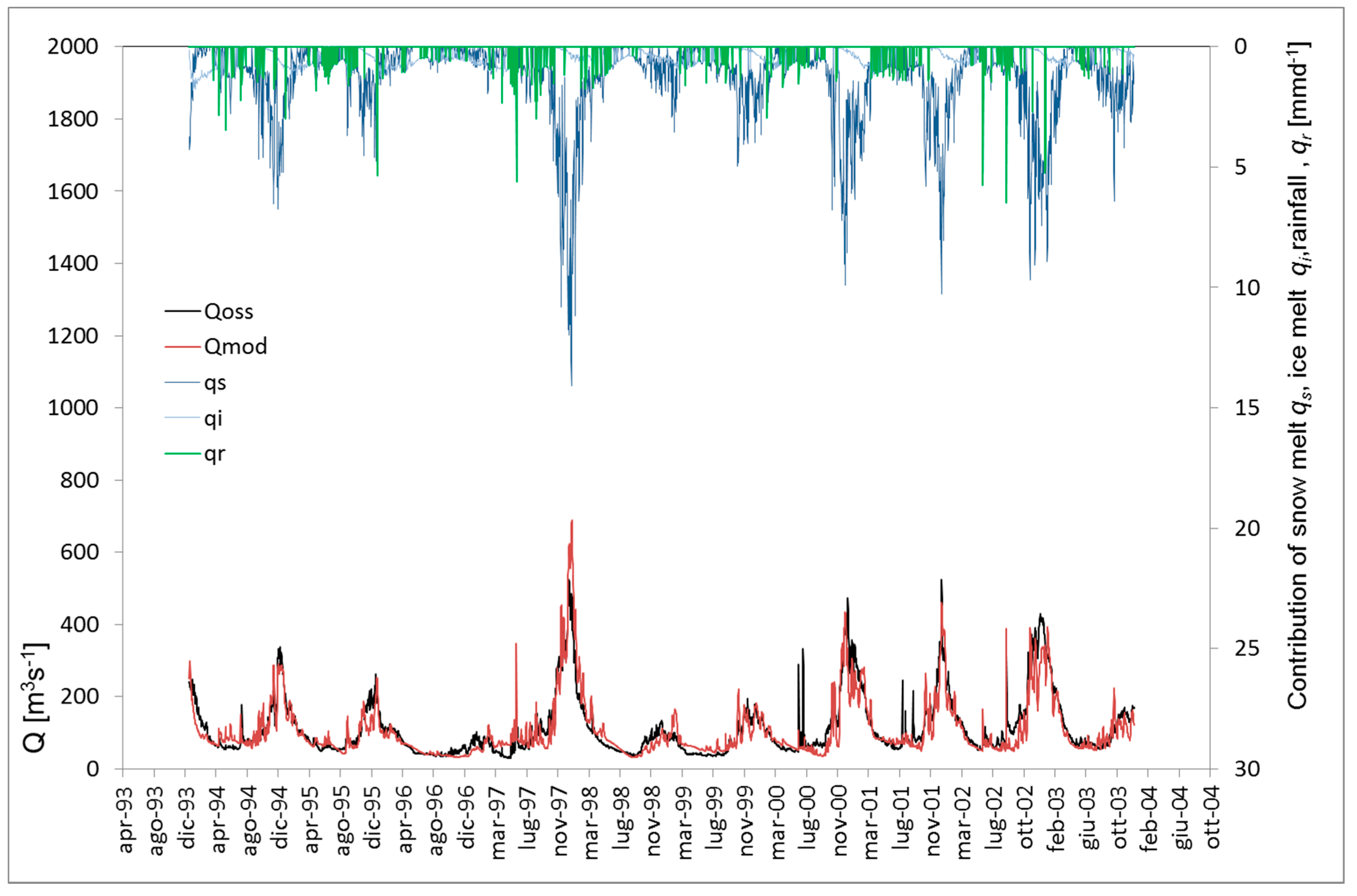
4.1. Models’ Performance

In Figure 2 we report calibration of Poly-Hydro (1994–2003, 2008–2011) at El Manzano, With Figure 3 giving validation. As reported in Figure 1b, model calibration was pursued by optimization of two goodness of fit measures, namely Bias (systematic error on average), and NSE (Nash-Sutcliffe Efficiency). We manually calibrated the model (see Table 3 for calibration parameters) to obtain a highest value of NSE (0 < NSE < 1 in general), constrained by a small Bias (i.e., |Bias| < 5%), so that, on average, the model depicted well water resource availability, and it also represents acceptably well their variability in time measured by NSE (see see [34] for some discussion about calibration of hydrological models in high altitude environment). In Table 3, we report calibration/validation statistics. Also in Figure 2 and Figure 3 we report daily flow components (precipitation, snow and ice melt). In Table 3 we also report statistics for calibration/validation without correction of ground temperature/rainfall with remote sensing (NSENS, RMSENS), and with use of the sole TRMM data (NSETR, RMSETR). We also report seasonal validation statistics, representing different flow generating mechanism (i.e., mostly snow melt during OND, ice melt during JFM, mixed during Fall, AMJ and Winter JAS). Generally, Poly-Hydro mimics acceptably seasonal flow dynamics. Snow melt factor was DD = 5.6 mm °C−1·day−1, close to that from snow data (DD = 5.9 mm °C−1·day−1 at Yerba Loca, DD = 6.5 mm °C−1·day−1 at San Francisco). The modelled monthly snow cover in Winter and Spring (JAS, OND, 2010–2012) was benchmarked vs. MOD10A2, with acceptable results (not shown). Ice melt factor was set to DD = 7.2 mm °C−1·day−1, larger than those observed upon our case study glaciers (DI = 4.1 mm °C−1·day−1 on San Francisco, DI = 2.6–4.5 mm °C−1·day−1 on Pyramid, depending on debris cover), and yet in line with values in literature [42,43,50]). In Figure 2 we report the flow contribution (mmd−1) from snow melt qs, ice melt qi, and rainfall qr (q = qs + qi + qr), indicating flow generation mechanism in different periods (see [34] for the importance of separating flow generation mechanisms). A large increase occurs during Spring (OND) due to snow melt, and subsequently ice melt increases flows in Summer (JFM), and Fall (AMJ). Rainfall sporadically contributes to flow during Winter (JAS). Yearly average during 1994–2003 from Poly-Hydro was E[qs] = 1.26 mm·day−1, E[qi] = 0.33 mm·day−1, E[qr] = 0.10 mm·day−1, i.e., snow melt contributes more than ice melt, and much more than rainfall.

4.2. Ice Flow Model

Poly-Hydro reproduces acceptably well the velocity field for both glaciers (see [18]). In Table 3, goodness of fit is reported. A Bias = −4% was observed, with determination coefficient RI2 = 0.56. Given this seemingly acceptable performance, we could use our model for description of ice flow of all glaciers in the area, for the purpose of hydrological modelling, and projections.

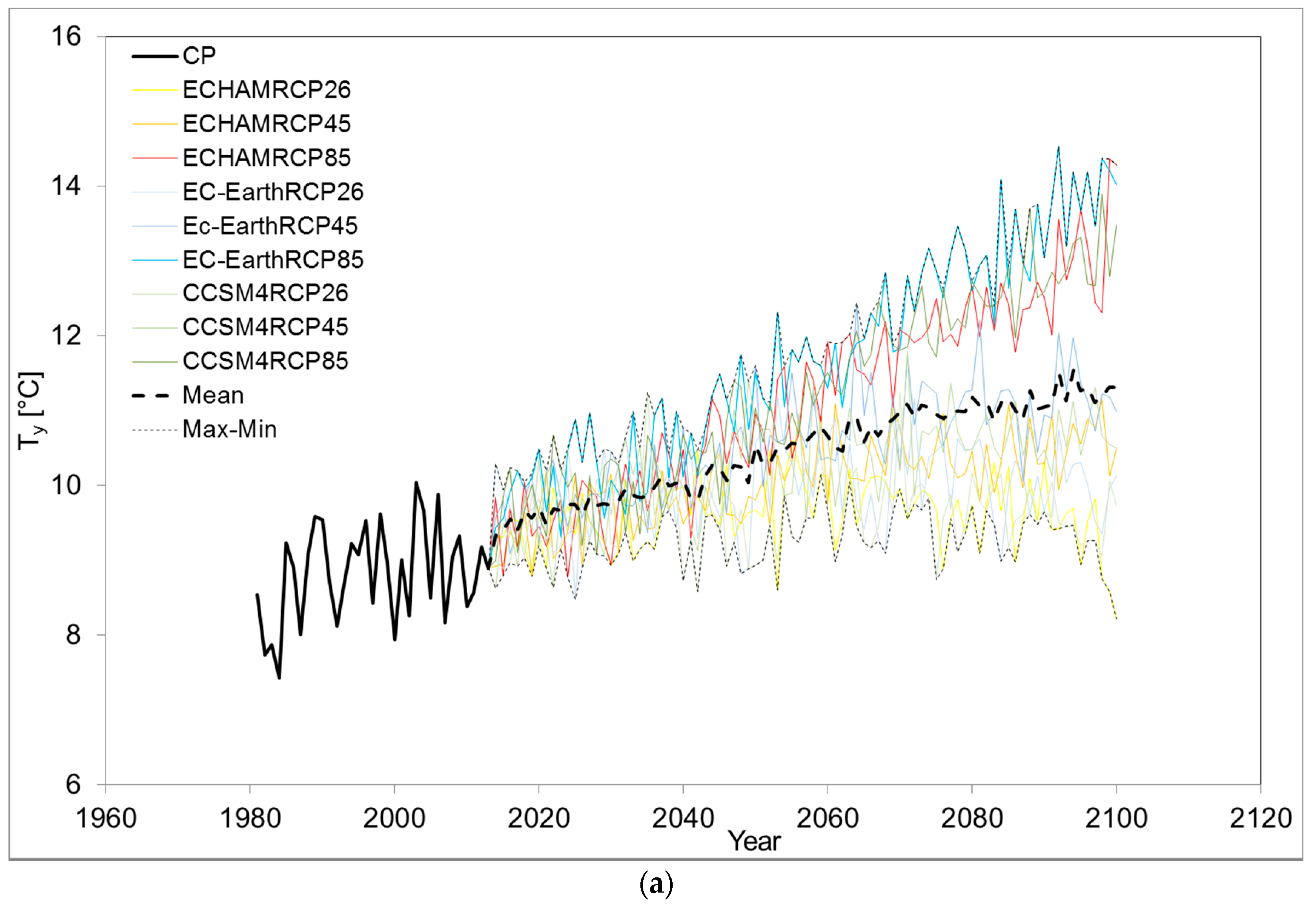
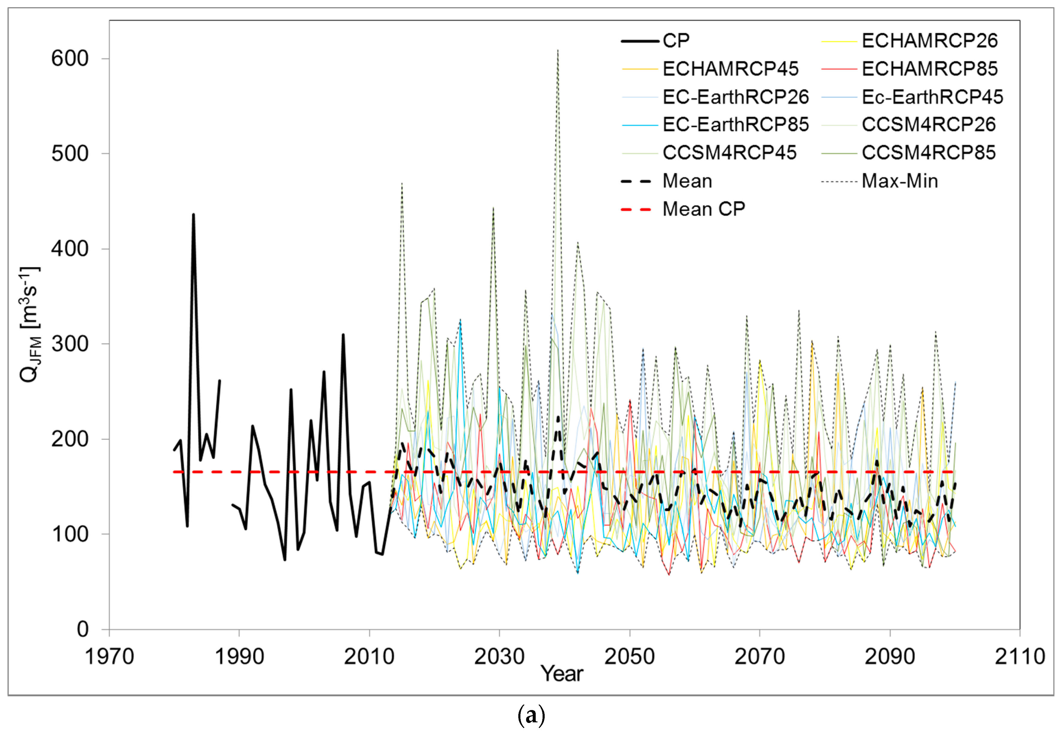
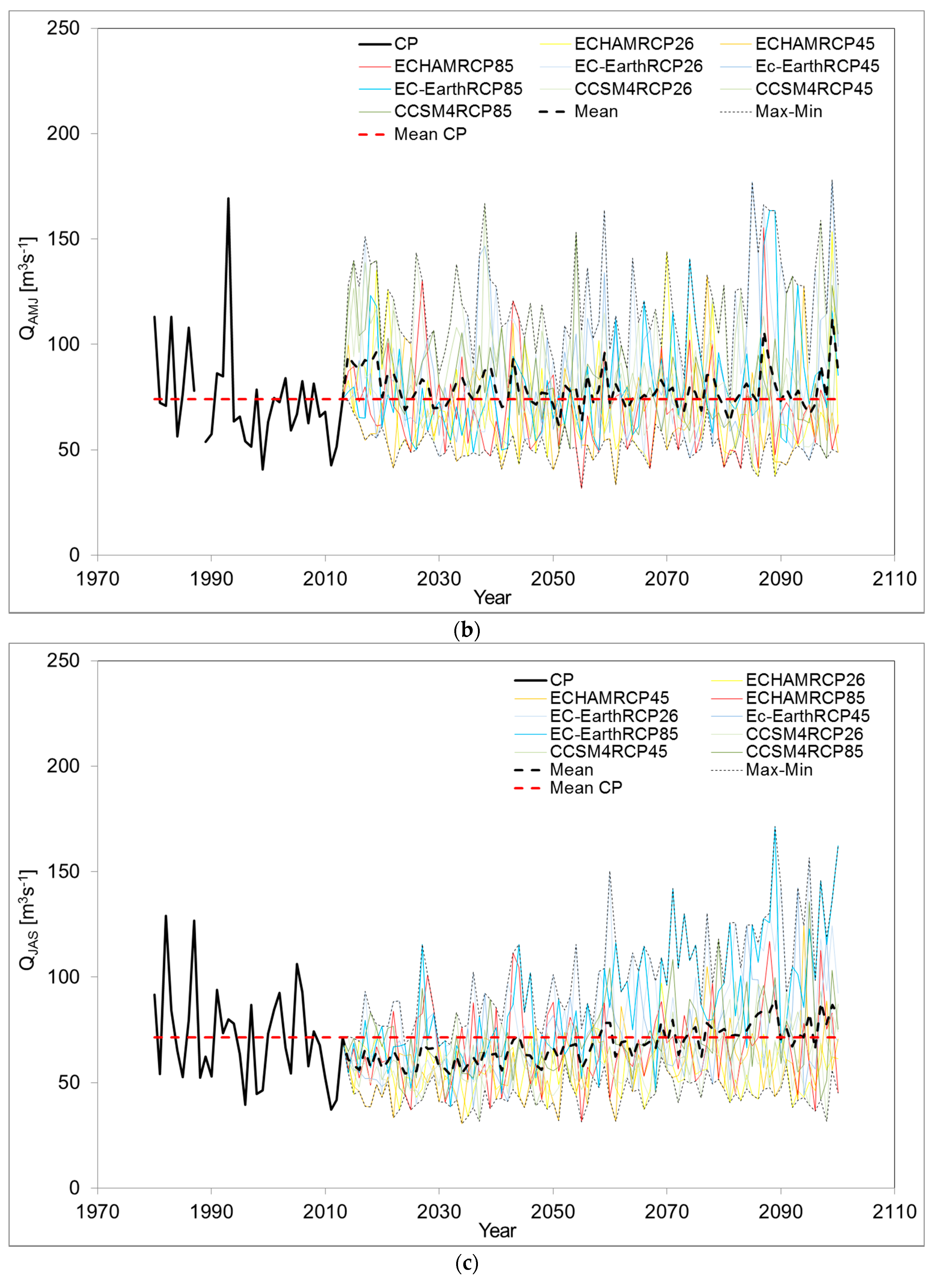
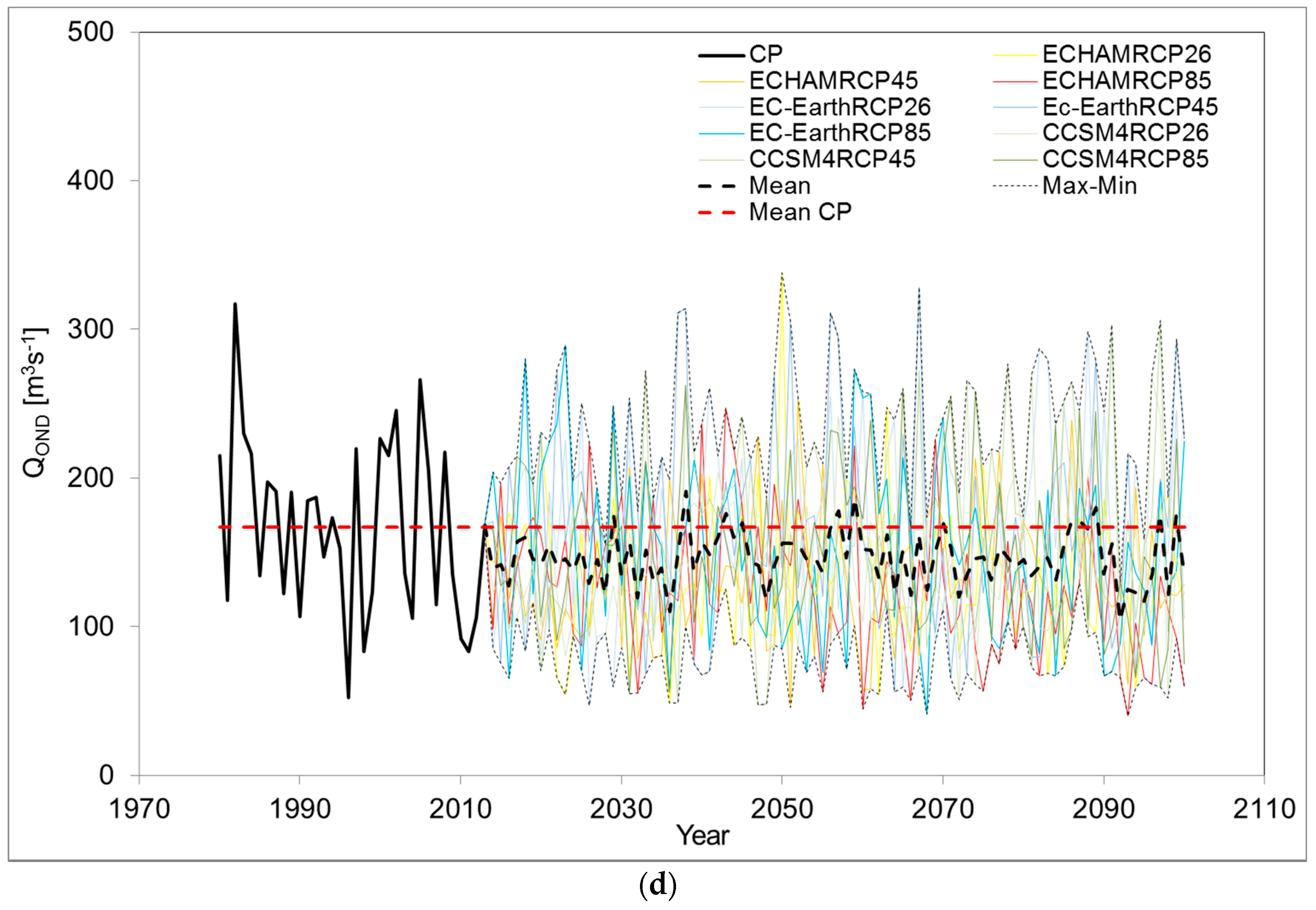
4.3. Climate and Hydrological Projections

In Figure 4a, we report projected yearly temperature until 2100, as from our three GCMs, and three RCPs (e.g., nine projections, plus mean value, and extremes), together with recent (CP 1981–2013) patterns, or control period CP. Also, yearly precipitation (mm·day−1) projections are reported in Figure 4b, including CP (1982–2013). Visibly, yearly temperature was rapidly increasing during CP, and until the end of the century (PR, 2014–2100), and similarly in all seasons (not shown). Precipitation instead was not visibly changing at the yearly scale, nor seasonally (not shown). Seasonal trends of temperature and precipitation under all scenarios were investigated in depth, reported in Section 4.5 below. Seasonal hydrological projections are reported in Figure 5, together with their CP (1980–2013) counterpart. During Summer (JFM, Figure 5a) decreases were seen in both CP, and PR under all scenarios. Fall (AMJ, Figure 5b), and Winter (JAS, Figure 5c) displayed visible decreases in CP, and increases in PR, and Spring (OND, Figure 5d) showed decreases in CP, and substantial stationarity in PR, on average. Again, seasonal trends of stream flows under all scenarios were investigated in depth, reported in Section 4.5 below.

4.4. Glaciers’ Dynamics

Figure 6 reports the past (1982–2013, CP) estimated glaciers’ depletion (i.e., ice volume) curve as obtained by back-estimation reported in Section 3.5, against potential future depletion under our climate scenarios. Also, potential ice evolution under present climate (stationary, STAT, is reported). Clearly after 2014, all GCMs models and RCPs projected a sudden increase of ice melting (i.e., a sudden loss in ice volume, as seen by the steeper curves in Figure 6). This was consistent with the large increase of temperature as simulated by all models (Figure 4a), and especially under RCP8.5. Particularly during Summer JFM, all models, and especially CCSM4, depicted large increases suddenly from 2014. Notice that all the GCMs used here provided projected series starting from 2006 (i.e., control runs end in 2005, and projections start in 2006, and no simulation is available starting after that year). Accordingly, projections from these GCMs may provide a large increase than actually happened in some regions, including here (i.e., making temperature in 2014 suddenly much higher than in 2013). As a result, in Figure 6 an abrupt transition is seen from the present behaviour (until 2013) to future dynamics (since 2014). However, this discontinuity only affects the curve locally, and does not impact on the long run glaciers’ dynamics. Indeed, glaciers’ down wasting as shown here is in response to increase of temperature in all seasons, especially Spring (OND), and Summer (JFM), which results into large ablation at higher altitudes than hitherto.

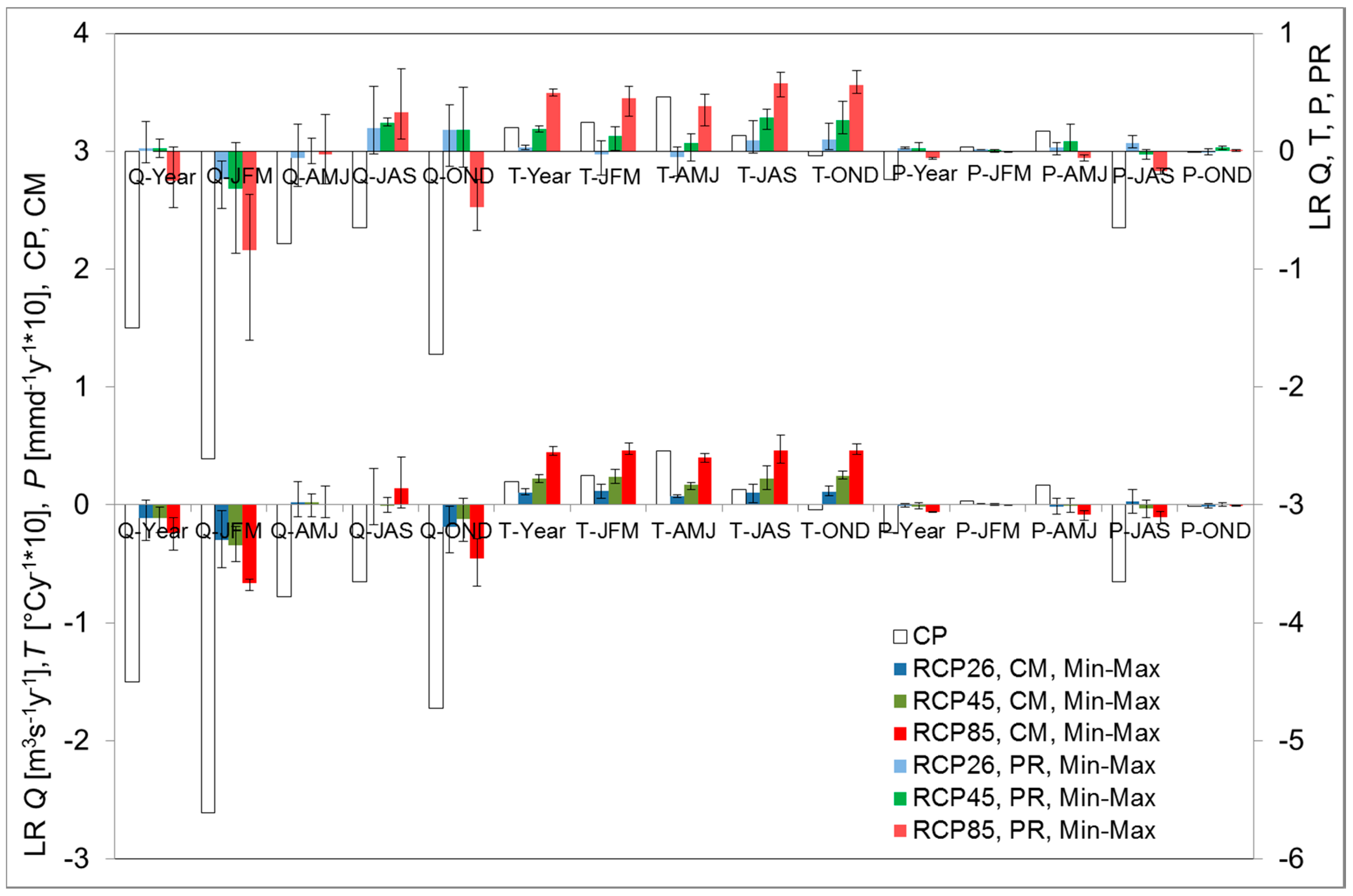
4.5. Climate and Hydrological Trends until 2100

We quantified climate and hydrological trends via linear regression (LR) during three periods, namely CP (1980–2013, for discharge, temperature, and precipitation), PR (2014–2100), and CM (CP+PR) In Table 4 we report seasonal indicators, including slope, and significance (α = 5%, bold values). In Figure 7 we resumed the so estimated trends of climate and hydrological fluxes for CP and CM situation, the latter of interest to gather a global (i.e., on a longer run) trend assessment, as per RCPs (average values and extremes), regardless of their significance. Also, the projected trends in PR period are reported in Figure 7. Temperature in Table 4 increased during CP (significantly in Summer JFM, and Fall AMJ), with a slight decrease during Spring OND. According to our nine scenarios (3 GCMs, three RCPs) T normally increased (mostly significantly) during all seasons. Decrease (significant) would be seen in few cases, in Summer and Fall under RCP2.6 of CCSM4. RCP2.6 depicts increase of temperature first (since 2014, until half century), then followed optimistically by mitigation of global warming, with decreasing temperature, as seen in Figure 4a. Decrease (not significant) occurred for RCP2.6 of EC-Earth during JAS. RCP4.5 of CCSM4 depicts significant decrease in Fall AMJ. When considering CM period, all scenarios depict significantly increasing temperature. Precipitation in CP decreased yearly, and during Winter JAS, and Spring AMJ, but never significantly. During PR and CM, precipitation was occasionally significantly increasing or decreasing, but no clear patterns were visible. Under RCP8.5, total (yearly), and Winter JAS precipitation decreased significantly. At the Y scale, decrease of flows (−1.5 m3·s−1·year−1) was observed in CP (1980–2013), and was statistically significant. From Figure 7, all models and scenarios (not RCP2.6 for ECHAM6) provided long run (CM, 1980–2100) decreasing yearly flows, and several significantly (all RCPs under CCSM4, RCP8.5 under Ec-Earth), with largest decrease projected at −0.39 m3·s−1·year−1 until 2100 under CCSM4, RCP8.5. This in spite of RCP2.6, and RCP4.5 projecting slightly increasing Q during PR (but RCP8.5 projecting large decrease on average, significant for CCSM4, and EC-Earth, and not significant increase for ECHAM6, Table 4). The largest flow changes would be during Summer, JFM. During CP significant flow decrease was detected (down to −2.6 m3·s−1·year−1), and CM scenarios project further decreasing discharge until 2100, mostly significantly (Figure 7, Table 4), and similarly during PR period (Table 4), unless for the case of CCSM4 (RCP4.5). During Fall AMJ, CP data provide not significant decrease, and all scenarios depict no changes therein on average. However, ECHAM for RCP2.6, and RCP8.5 projects significant increase during PR period (and also during CM), while EC-Earth under RCP2.6, and RCP8.5 project significant decrease during CP (but not CM), from Table 4. In Winter JAS, no significant decrease was detected in CP. During PR all scenarios project large flow increase in Winter (except for EC-Earth under RCP2.6, with very slight decrease), in most cases significantly (CCSM4 in RCP4.5, ECHAM6 all RCPs, EC-Earth under RCP4.5 and RCP8.5). Given however the observed decrease in CP, on the long run of CM, more stable JAS flows were projected (with significant decrease under CCSM4 for RCP2.6, and significant increase for ECHAM6 under RCP2.6, and RCP8.5). During Spring OND, a somewhat large (albeit not significant, p-val = 0.10) flow decrease was seen in the CP period. During PR, discharges increased on average under RCPs 2.6 and 4.5, but decreased for RCP8.5 (significantly for CCSM4 and ECHAM6). However, on the long run Spring flow always decreased until the end of the century (and significantly in most cases, e.g., all RCPs for CCSM4, RCP8.5 for ECHAM6, and EC-Earth).

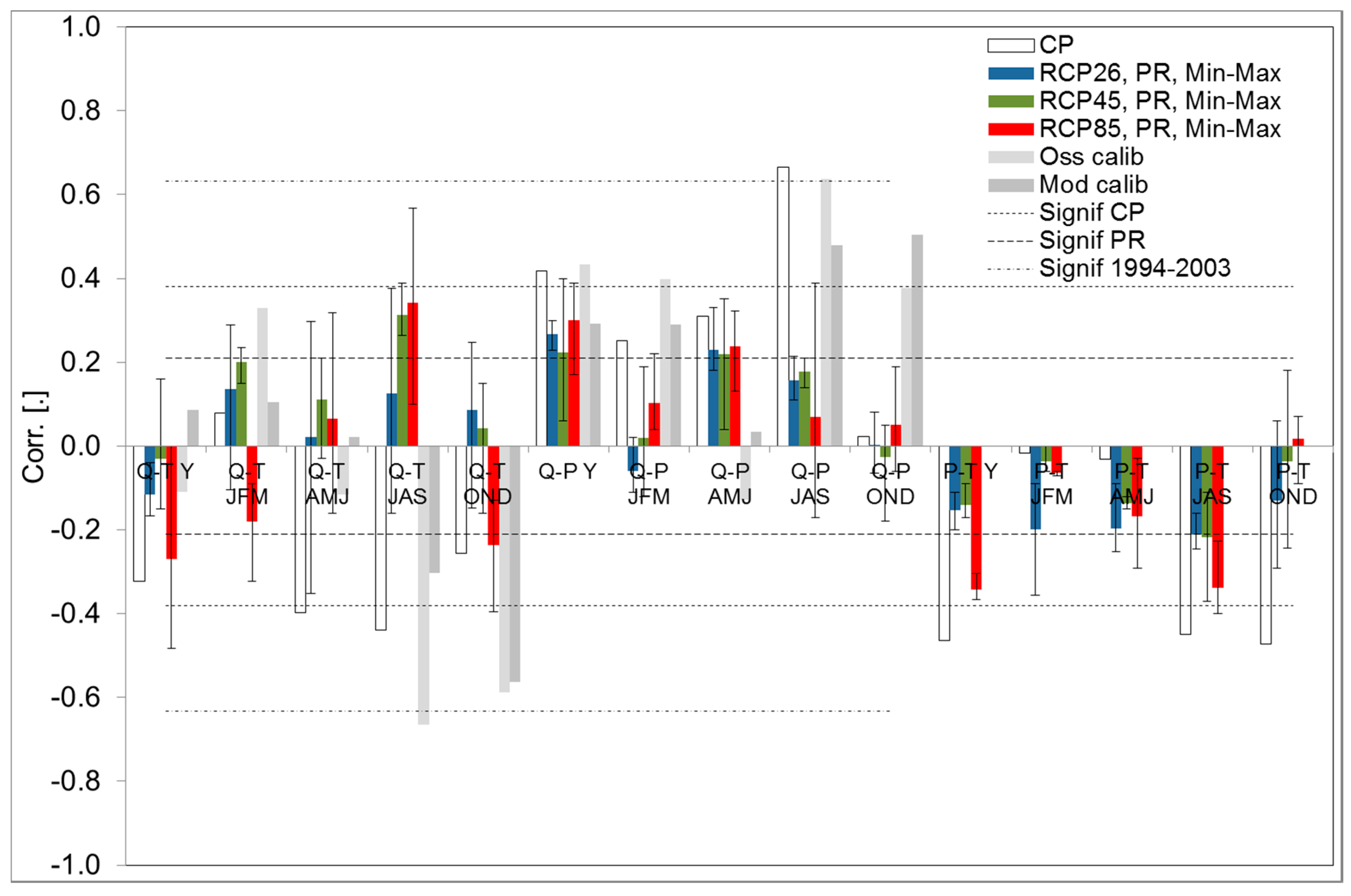
4.6. Correlation against Climate Drivers

In Table 5, we report the yearly and seasonal correlation analysis between climate (temperature T, precipitation P) and hydrological (discharge Q) variables during past (1982–2013 for all series for consistency), and projected (PR 2014–2100) periods. Only first order correlation analysis was pursued (i.e., same year, same season) for simplicity. In Figure 8 we provide a resume for CP, and PR, as per RCPs, with indication of significance. In grey shades we report correlation analysis during model calibration period (1994–2003) to test consistence of climate to hydrology correlation in modelled and observed series, i.e., to (i) verify if modelled series display a correlation with climate similar to the observations during the same periods, necessary for making usable inferences for the future, and (ii) avoid correlation highlighted by the model which has no correspondence in the actual flow regime. This exercise indicated that the modelled discharges substantially displayed coherent correlation with the observed ones (albeit with less significance in some cases), so that one can use, for indicative purposes, correlation analysis upon modelled variables to investigate potential the future correlation of in stream flows against climate drivers. During CP, normally anti-correlation between flows and temperature was seen, and it was especially significant in Fall AMJ, and Winter JAS. Conversely, precipitation was positively correlated with stream flows, especially in Winter. Also, clear anti-correlation was seen between precipitation, and temperature, yearly, but especially in Winter (when ca. 45% of yearly precipitation occurs, Table 4), and Spring, however dry. Accordingly, hot Winters may lead to low precipitation income. In the PR period, mostly the observed correlations were confirmed. Precipitation will be largely (and mostly significantly) anti-correlated against temperature during the wettest Winter season, and also yearly, especially under RCP8.5. Consistently, as reported above, yearly, and Winter precipitation would always decrease significantly under RCP8.5. Also, projected flows would be mostly positively correlated to precipitation, especially during Fall AMJ, and less during Winter under RCP8.5 (however variable). A small and not significant correlation, Q vs. P, would be seen during Summer, and Spring, however very dry as reported, was not projected to change in the future. More variable seems the correlation of stream flows against temperature in the future. While at the yearly scale stream flow remained negatively (and significantly on average) correlated against temperature as seen during CP, seasonally some changes may occur. During Summer JFM, RCP26, and RCP4.5 projected increasingly positive correlations of Q vs. T, according to what was found during CP. However, under RCP8.5, anti-correlation was projected. Similarly occurs during Fall AMJ, when small positive correlation coefficients were projected on average, against the significantly negative correlation during CP. Also in Winter, large and often significant (see Table 5) positive correlation coefficients are found between Q and T, increasingly with the RCP, and conversely to CP. During Spring OND, mostly not significant correlation was projected, except for some anti-correlation under RCP8.5. Accordingly, the projected correlation structure between flow and its climate drivers in the Maipo River mirrors partially the results found investigating the historical series, and some changes were seen. Such modified correlation structure may derive from the underlying patterns of flow formation, as driven by climate, and requires some discussion, which we report below.

5. Discussion

5.1. Glacio-Hydrological Trends, and Flow Components

The Poly-Hydro model provides an acceptable description of the stream flows in the Maipo River. Seasonal flows were acceptably simulated both in calibration, and validation phase. One may therefore confidently project forward the catchment response to future climate trends, in the hypothesis of unchanged response patterns. To complement our analysis with explicit investigation of flow components and hydrological fluxes, in Figure 9 we report, for the CP and PR periods, the (average seasonal, per scenarios) relative contribution (averaged at the catchment scale) to in stream flows of snow, and ice melt (lumped). This includes melt ratio Mr = (qi + qs)/q, rainfall ratio, or the share of stream flow given by rainfall Rr = 1 − Mr, and evapotranspiration ratio as ETr = ET/(R + Mi + Ms). Joint analysis of trends and correlations (Figure 7 and Figure 8) with Figure 6 providing ice ablation, and Mr and ETr in Figure 9 may provide an explanation of the observed and projected trends of stream flows into the Maipo River under past, and projected future climate conditions. During Summer JFM, flow decrease was projected in the future, continuing the observed significant trends of the recent past (CP period, Figure 7). During CP, no significant trend of P was seen in Summer (slight increase is detected), while T increased significantly (Table 4). From Figure 8 (and Table 5), Q was not significantly correlated to T or P. From Figure 9a, during RCP Mr was constant and nearby 0.99 on average. Snow melt was substantially constant (no large precipitation changes are detected anywhere, Figure 7), and ice depletion occurs during Summer (Figure 2), so the decrease of Q during JFM may likely be due to decreased ice melt (i.e., for lack of ice), say since 1990s’ as calculated from our model, and reported in Figure 6. During PR, QJFM further decreases, especially under RCP8.5 (Figure 7). For RCP 2.6 and RCP4.5 positive correlation of QJFM vs. temperature was seen, and conversely for RCP8.5 (Figure 8). Figure 6 indicates that initially in PR increasing ice melt was seen due to increasing temperature, but lather decrease occurs especially under RCP2.6 and RCP4.5. From Figure 9a on the long run Mr would decrease slightly, and ETr would increase instead, especially for RCP8.5. Accordingly stream flows during JFM would largely depends on snow and ice melt, the latter decreasing with time. Increasing ETr driven by temperatures (especially under RCP8.5) would further decrease stream flow (hence, anti-correlation of Q vs. T in Figure 8). In Fall AMJ, the same trends as in JFM persist. Ice melt would occur in Fall (Figure 2), and decreasing ice melt since the 90s’ (Figure 6) may have reduced QAMJ in the CP period. Also, the slightly increasing ETr (due to significantly increasing T, Table 4) may have further decreased stream flows (again here, see anti-correlation of Q vs. T in Figure 8). In the PR period, AMJ would be substantially constant. Melt ratio Mr would decrease at the end of century given decreasing ice melt, still higher than now (and constant snow melt, not shown). ETr would increase due to high temperatures (especially under RCP8.5). However, sustained melting from higher temperatures would still maintain stream flows at the present level during Fall for most of the century. During Winter JAS no significant trend was detected during CP. Stream flows slightly decreased during CP, possibly due to decreased precipitation (Table 4), and also given large significant correlation coefficient of Q vs. P in JAS (Figure 8). QJAS would slightly increase during PR period, with an eventually stationary behaviour. During PR, both ice and snow melt would increase due to increasing T, and being rainfall substantially constant, Mr would increase (Figure 9c). Increasing ETr in response to increasing T would not be able to offset increased melting, and Winter stream flows would increase at the end of the century.
In Spring OND, historical discharge decreased visibly (albeit not significantly, Table 4, p-val = 0.09), in spite of substantially constant T and P (no visible correlation of Q is seen vs. either). Analysis of ice melt during Spring (not shown) displayed decreasing values during CP, consistent with ice volume decreasing as from Figure 6, which with substantially constant snow melt, may explain decreasing Q. In the PR period, a similar pattern would be seen during Summer JFM. Namely, under RCP2.6 and RCP4.5, higher temperature and increasing ice melt (Figure 6) would lead to high Mr, and to increasing flows (hence, positive albeit small correlation of Q vs. T for OND in Figure 8, RCP2.6, RCP4.5) towards the end of the century (yet with a negative net balance during CM). Under RCP8.5 however, increasing temperature would also largely increase ETr (Figure 9d), thus providing decreasing QOND during CP (and significantly negative correlation of Q vs. T for OND in Figure 8, RCP8.5).
At the yearly scale, the projected trends would be consistent with past observations. During CP, significant flow decrease has been detected, given by decreased ice melt since the 90s, and possibly increasing evapotranspiration (as displayed by negative, albeit not significant correlation of Q vs. T for Y in Figure 8, CP). The projected trends indicate substantially constant, or slightly decreasing flows as given trading off by initial increased ice melting, followed by decreasing ice availability, and increasing evapotranspiration, especially under RCP8.5, with the largest negative correlation coefficient Q vs. T (Figure 8, Table 5, Y).
Eventually, the projected scenarios indicate evolution of the hydrology of the Maipo River as dominated by temperature increase, with a twofold effect of increasing ice and snow melt (the latter being faster, but substantially constant at the yearly scale given slight changes in precipitation), and changing ice melt availability, initially larger given the rise of temperature (and altitude of the melting area), but lately smaller for depletion, with evapotranspiration becoming more effective. On average (nine scenarios), at the end of the century, yearly mean discharge would change from 120 m3·s−1 now, to 106 m3·s−1 (−11.3%) at 2100, with a variability between 82 m3 s−1 and 128 m3 s−1 (−32% to +7%).

5.2. Benchmark against the Present Literature

The authors of [6] studied the Juncal Norte glacier, North of Maipo here. With climate scenarios from 2 GCMs (ECHAM5, HadCM3, AR4 of IPCC, 2007) under storyline A1B (medium optimistic) they projected mass balance of Juncal at 2050. Yearly, they projected runoff at −30% under HadCM3, but constant under ECHAM5 ([6], Figure 8). Until 2050 we depicted (Figure 5, decade 2045–2054) a change (vs. 1980–2013) of −11% on average, from +3% (EC-Earth, RCP4.5) to −24% (EC-Earth, RCP8.5). The authors in [6] did not include ice flow, resulting in accumulation at high altitude being unreasonable (see also [26]), and into ablation tongues rapidly down wasting, nor they included evapotranspiration, influencing the water budget under the warmest scenarios. In [13], the authors studied effects of climate change until 2065 on the Maipo River at El Manzano, also based on CEPAL [51]. They projected monthly flows during 2035–2065 to −12% yearly, similarly to here (here −8% on average for the same years, lowest −22%, highest +2.5%). The authors of [12] used a multisite stochastic weather generator to downscale A2 and B2 scenarios, and a hydrological model including crop production to simulate monthly flows at El Manzano for 2071–2100. They projected largely increased (ca. +15%) evapotranspiration like we did here (Figure 9). They further report that during irrigation season (OND+JFM) flow decrease would affect the area. Our runoff estimates for 2071–2100 during irrigation season provide on average −17% (lowest −38%, highest +3%). Krellenberg and Hansjürgens [52] studied water availability in the Maipo based on AR5 projections, and predicted, until 2050, a potential decrease from −19% (B1 storyline) to −30% (A2 storyline), even larger than our RCP4.5 (−8% on average), and RCP8.5 (−15% on average). Our results here are consistent with the available literature (see also [53]), and yet updated (i.e., based upon more recent climate projections form AR5 of IPCC), and physically based (i.e., on a hydrological model including the main physical processes governing water budget, and flow components).

5.3. Limitations and Outlooks

The present work has limitations. Permafrost and rock glaciers dwell in the Maipo catchment [5,54], and were not modelled here. Hydrological dynamics of permafrost, i.e., of the active layer [55,56] needs to be studied in situ, and no knowledge was available that we know of in the case study area. A simple melt model (degree-day) was used here for cryospheric flows, when more complex methods may be used, including mixed (e.g., with solar radiation) temperature index models [5,34], or energy budget models [28]. However, degree day models at the daily scale provide acceptable results for hydrological purposes [15,57], at the cost of limited data requirement, conversely to other more demanding methods (e.g., [58]). We lumped degree day of ice regardless of debris cover, given lack of debris thickness information for glaciers (as used e.g., in [15,26,59]. Marangunic [60] reported glaciers in the Rio Maipo (above Las Melosas, Figure 1) to possess ca. 44% debris cover. DGA [44] more recently reported in the whole catchment 43% debris cover. The large size of cells in Poly-Hydro model (3 × 3 km2), necessary for computational reasons may have hidden the variability of glaciers’ dynamics. However, we used partial cell coverage, and visually analysed flow velocity and ice flow dynamics, found to be consistent with those measured in situ, and acceptable thickness and shear stress during the simulation [18]. Uncertainty may occur in the initial (2012) ice thickness provided by DGA [40]. At El Manzano in 2012, we mapped 341 km2 of ice cover, and an estimated volume of 25.2 km3 of water (i.e., ca. a mean 74 m thickness). DGA [44] for the whole Maipo catchment mapped ca. 388 km2, and estimated a volume of ca. 37 km3 (i.e., ca. a mean 96 m in thickness), largely variable depending on the estimation method. In spite of changes in the absolute thickness (affecting slightly ice flow dynamics), relative thickness change seems large especially under the warmest scenarios, and the broad picture seems not largely affected by the initial conditions. Our back estimation of ice (water) volume at 1982 was indicative. We obtained 29.1 km3 in 1982 (ca. 85 m thickness on average), while Marangunic [60] estimated for the Maipo superior (much smaller) ca. 67 km2, and ca. 3.4 km3 of water (ca. 51 m in thickness), comparable given large uncertainty of estimation.
Variability of climate projections from different models, especially for precipitation (e.g., [35] for Italy, [15] in the Karakoram, [16,61] for the Himalayas) may influence the results. Seasonal temperature patterns here are consistent between models, but more variability is seen in precipitation. Here, until 2100, a decrease of precipitation was projected on average, and the more so with the warmer RCPs. Largest changes would happen in Fall and Winter, which are the two wet seasons (Table 4). Future steps may include sensitivity analysis against climate projections, e.g., using synthetic simulation (e.g., ensembles of climate patterns based upon GCM scenarios, e.g., [35]) beyond our scope in this manuscript. Even with uncertainty as reported, our results depict consistent pattern, in line with the present know how concerning future hydrology of the central Andes of Chile.

6. Conclusions

Our study assessed impacts of climate change on water resources, and hydrological components in the Maipo catchment of Santiago under updated climate scenarios from the AR5 of IPCC until 2100. During three decades recently Maipo underwent visible flow decrease yearly, most notably in Spring and Summer, when water is needed for irrigation. Decreasing trends were envisioned for the future in those seasons, and more under the warmest RCPs towards mid-century, when ice cover would be largely thinned, and evapotranspiration would draw large amount of moisture. Glacier cover would be increasingly depleted with rising of melting altitude, providing initially more water, but less water after. Stream flows would increase at the cost of ice down wasting during dry, increasingly warmer Fall and especially Winter, but the net effect would be flow decrease. Recent findings [62] indicate that global temperature, when compared against GCMs projections under IPCC AR5 launched in 2006, substantially overlaps with the projected pattern under RCP8.5, i.e., warming proceeded according to the most pessimistic scenario. Seemingly thus, if projections need be made now, globally one may expect that most credible scenarios here are those under RCP8.5. Notwithstanding uncertainty, our results seem consistent, and credible, also in the face of the present literature. Policy makers in Chile are therefore warned, climate change is acting, and will further act to decrease water availability in this region, and deplete ice cover, so that adaptation needs be tackled rapidly enough.

Author Contributions

D.B., field campaigns and data gathering, project coordination, paper writing. A.S., model set up and tuning, management of climate projections. A.S., field campaigns, glaciological data elaboration. G.D., project coordination, glaciologial model set up, paper writing.

Acknowledgments

The present work is in fulfilment of, and received funding from the project: “Cooperación técnica no reembolsable ATN/OC-11996 Chile, Programa plan de acción para la conservación de glaciares ante el cambio climático”, Dirección General de Aguas, Ministerio de Obras Públicas, carried out during January–December 2012. We acknowledge F. Migliavacca and G. Confortola for aid in setting up Poly-Hydro model. We acknowledge G. Barcaza, and the Dirección General de Aguas for support during the project. Grant awarded to EVK2CNR, under scientific coordination of G. Diolaiuti. EVK2CNR, and most notably Luca Listo is kindly acknowledged for project’s management, and logistic support. We acknowledge the World Climate Research Programme’s Working Group on Coupled Modelling, which is responsible for CMIP and we thank the MPI-ESM for producing and making available their model outputs. The MODIS and TRMM data products are courtesy of the online Data Pool at the NASA Land Processes Distributed Active Archive Center (LP DAAC), USGS/Earth Resources Observation and Science (EROS) Center, Sioux Falls, South Dakota. The elaborations for this manuscript were performed in the Climate-Lab environment of Politecnico di Milano.

Conflicts of Interest

The authors declare no conflict of interest.

References

  1. Rivera, A.; Acuña, C.; Casassa, G.; Bown, F. Use of remote sensing and field data to estimate the contribution of Chilean glaciers to the sea level rise. Ann. Glaciol. 2002, 34, 367–372. [Google Scholar] [CrossRef]
  2. Rivera, A.; Bown, F.; Acuña, C.; Ordenes, F. I Ghiacciai del Cile come Indicatori dei Cambiamenti Climatici. Chilean Glaciers as Indicators of Climatic Change. Terra Glacialis Edizione Speciale. Special Issue “Mountain Glaciers and Climate Changes in the Last Century”. 2009. Available online: http://repositorio.uchile.cl/bitstream/handle/2250/117817/113801_C11_rivera-italia.pdf?sequence=1 (accessed on 24 June 2018).
  3. Urrutia, R.; Vuille, M. Climate change projections for the tropical Andes using a regional climate model: Temperature and precipitation simulations for the end of the 21st century. J. Geophys. Res. 2009, 114, 2156–2202. [Google Scholar] [CrossRef]
  4. Bodin, X.; Rojas, F.; Brenning, A. Status and evolution of the cryosphere in the Andes of Santiago. Geomorphology 2011, 118, 453–464. [Google Scholar] [CrossRef]
  5. Pellicciotti, F.; Helbing, J.; Rivera, A.; Favier, V.; Corripio, J.; Araos, J.; Sicart, J.-E.; Carenzo, M. A study of the energy balance and melt regime on Juncal Norte Glacier, semi-arid Andes of central Chile, using melt models of different complexity. Hydrol. Process. 2008, 22, 3980–3997. [Google Scholar] [CrossRef]
  6. Pellicciotti, F.; Ragettli, S.; Carenzo, M.; McPhee, J. Review: Changes of glaciers in the Andes of Chile and priorities for future work. Sci. Total Environ. 2014, 493, 1197–1210. [Google Scholar] [CrossRef] [PubMed]
  7. Rabatel, A.; Castebrunet, H.; Favier, V.; Nicholson, L.; Kinnard, C. Glacier changes in the Pascua-Lama region, Chilean Andes (29S): Recent mass balance and 50 yr surface area variations. Cryosphere 2011, 5, 1029–1041. [Google Scholar] [CrossRef] [Green Version]
  8. Rabatel, A.; Francou, B.; Soruco, A.; Gomez, J.; Caceres, B.; Ceballos, J.L.; Basantes, R.; Vuille, M.; Sicart, J.-E.; Huggel, C.; et al. Current state of glaciers in the tropical Andes: A multi-century perspective on glacier evolution and climate change. Cryosphere 2013, 7, 81–102. [Google Scholar] [CrossRef] [Green Version]
  9. Carrasco, J.F.; Casassa, G.; Quintana, J. Changes of the 0 °C isotherm and the equilibrium line altitude in central Chile during the last quarter of the 20th century. Hydrol. Sci. J. 2005, 50, 933–948. [Google Scholar] [CrossRef]
  10. Masiokas, M.H.; Villalba, R.; Luckman, B.H.; Le Quesne, C.; Aravena, J.C. Snowpack Variations in the Central Andes of Argentina and Chile, 1951–2005: Large-Scale Atmospheric Influences and Implications for Water Resources in the Region. J. Clim. 2006, 19, 6334–6352. [Google Scholar] [CrossRef]
  11. Masiokas, M.H.; Rivera, A.; Espizua, L.E.; Villalba, R.; Delgado, S.; Aravena, J.C. Glacier fluctuations in extratropical South America during the past 1000 years. Palaeogeogr. Palaeoclimatol. Palaeoecol. 2009, 281, 242–268. [Google Scholar] [CrossRef]
  12. Meza, F.J.; Wilks, D.S.; Gurovich, L.; Bambach, N. Impacts of Climate Change on Irrigated Agriculture in the Maipo Basin, Chile: Reliability of Water Rights and Changes in the Demand for Irrigation. J. Water Resour. Plan. Manag. 2012, 138, 421–430. [Google Scholar] [CrossRef]
  13. Ahumada, G.; Bustos, D.; González, M. Effect of climate change on drinking water supply in Santiago de Chile. Sci. Cold Arid Reg. 2013, 5, 27–34. [Google Scholar]
  14. Bocchiola, D.; Mihalcea, C.; Diolaiuti, G.; Mosconi, B.; Smiraglia, C.; Rosso, R. Flow prediction in high altitude ungauged catchments: A case study in the Italian Alps (Pantano Basin, Adamello Group). Adv. Water Resour. 2010, 33, 1224–1234. [Google Scholar] [CrossRef]
  15. Soncini, A.; Bocchiola, D.; Confortola, G.; Bianchi, A.; Rosso, R.; Mayer, C.; Lambrecht, A.; Palazzi, E.; Smiraglia, C.; Diolaiuti, G. Future hydrological regimes in the upper Indus basin: A case study from a high altitude glacierized catchment. J. Hydrometeorol. 2015, 16, 306–326. [Google Scholar] [CrossRef]
  16. Soncini, A.; Bocchiola, D.; Confortola, G.; Minora, U.; Vuillermoz, E.; Salerno, F.; Viviano, G.; Shrestha, D.; Senese, A.; Smiraglia, C.; et al. Future hydrological regimes and glacier cover in the Everest region: The case study of the Dudh Koshi basin. Sci. Total Environ. 2016, 565, 1084–1101. [Google Scholar] [CrossRef] [PubMed]
  17. Aili, T.; Soncini, A.; Bianchi, A.; Diolaiuti, G.; Bocchiola, D. A method to study hydrology of high altitude catchments: The case study of the Mallero River, Italian Alps. Theor. Appl. Climatol. 2018, 1–22. [Google Scholar] [CrossRef]
  18. Migliavacca, F.; Confortola, G.; Soncini, A.; Diolaiuti, G.A.; Smiraglia, C.; Barcaza, G.; Bocchiola, D. Hydrology and potential climate changes in the Rio Maipo (Chile). Geogr. Fis. Din. Quat. 2015, 38, 155–168. [Google Scholar]
  19. Peel, M.C.; Finlayson, B.L.; McMahon, T.A. Updated world map of the Köppen-Geiger climate classification. Hydrol. Earth Syst. Sci. 2007, 11, 1633–1644. [Google Scholar] [CrossRef]
  20. Garreaud, R.; Aceituno, P. Interannual rainfall variability over the South American Altiplano. J. Clim. 2001, 14, 2779–2789. [Google Scholar] [CrossRef]
  21. Bookhagen, B.; Burbank, D.W. Topography, relief, and TRMM-derived rainfall variations along the Himalaya. Geophys. Res. Lett. 2006, 33, L08405. [Google Scholar] [CrossRef]
  22. Bookhagen, B.; Burbank, D.W. Towards a complete Himalayan hydrologic budget: Thespatiotemporal distribution of snow melt and rainfall and their impact on river discharge. J. Geophys. Res. 2010. [Google Scholar] [CrossRef]
  23. Bocchiola, D. Use of Scale Recursive Estimation for multisensor rainfall assimilation: A case study using data from TRMM (PR and TMI) and NEXRAD. Adv. Water Resour. 2007, 30, 2354–2372. [Google Scholar] [CrossRef]
  24. Parajka, J.; Blöschl, G. The value of MODIS snow cover data in validating and calibrating conceptual hydrologic models. J. Hydrol. 2008, 358, 240–258. [Google Scholar] [CrossRef]
  25. Parajka, J.; Blöschl, G. Spatio-temporal combination of MODIS images-potential for snow cover mapping. Water Resour. Res. 2008, 44. [Google Scholar] [CrossRef]
  26. Bocchiola, D.; Diolaiuti, G.; Soncini, A.; Mihalcea, C.; D’Agata, C.; Mayer, C.; Lambrecht, A.; Rosso, R.; Smiraglia, C. Prediction of future hydrological regimes in poorly gauged high altitude basins: The case study of the upper Indus, Pakistan. Hydrol. Earth Syst. Sci. 2011, 15, 2059–2075. [Google Scholar] [CrossRef] [Green Version]
  27. Mihalcea, C.; Mayer, C.; Diolaiuti, G.; Lambrecht, A.; Smiraglia, C. Ice ablation and meteorological conditions on the debris covered area of Baltoro Glacier, Karakoram (Pakistan). Ann. Glaciol. 2006, 43, 292–300. [Google Scholar] [CrossRef]
  28. Bocchiola, D.; Senese, A.; Mihalcea, C.; Mosconi, B.; D’Agata, C.; Smiraglia, C.; Diolaiuti, G. An ablation model for debris covered ice: The case study of Venerocolo Glacier (Italian Alps). Geogr. Fis. Din. Quat. 2015, 38, 113–128. [Google Scholar]
  29. Intergovernmental Panel on Climate Change (IPCC). Summary for Policymakers. In Climate Change 2013: The Physical Science Basis. Contribution of Working Group I to the Fifth Assessment Report of the Intergovernmental Panel on Climate Change; Stocker, T.F., Qin, D., Plattner, G.-K., Tignor, M., Allen, S.K., Boschung, J., Nauels, A., Xia, Y., Bex, V., Midgley, P.M., Eds.; Cambridge University Press: Cambridge, UK; New York, NY, USA, 2013. [Google Scholar]
  30. Gent, P.R.; Danabasoglu, G.; Donner, L.J.; Holland, M.M.; Hunke, E.C.; Jayne, S.R.; Lawrence, D.M.; Neale, R.B.; Rasch, P.J.; Vertenstein, M.; et al. The Community Climate System Model Version. J. Clim. 2011, 24, 4973–4991. [Google Scholar] [CrossRef]
  31. Hazeleger, W.; Wang, X.; Severijns, C.; Ştefănescu, S.; Bintanja, R.; Sterl, A.; Wyser, K.; Semmler, T.; Yang, S.; van den Hurk, B.; et al. EC-Earth V2.2: Description and validation of a new seamless earth system prediction model. Clim. Dyn. J. 2011, 39, 2611–2629. [Google Scholar] [CrossRef]
  32. Stevens, B.; Giorgetta, M.; Esch, M.; Mauritsen, T.; Crueger, T.; Rast, S.; Salzmann, M.; Schmidt, H.; Bader, J.; Block, K.; et al. Atmospheric component of the MPI-M Earth System Model: ECHAM. J. Adv. Model. Earth Syst. 2013, 5, 1–27. [Google Scholar] [CrossRef]
  33. Groppelli, B.; Bocchiola, D.; Rosso, R. Spatial downscaling of precipitation from GCMs for climate change projections using random cascades: A case study in Italy. Water Resour. Res. 2011, 47, W03519. [Google Scholar] [CrossRef]
  34. Soncini, A.; Bocchiola, D.; Azzoni, R.S.; Diolaiuti, G. A methodology for monitoring and modeling of high altitude Alpine catchments. Prog. Phys. Geogr. 2017, 41, 393–420. [Google Scholar] [CrossRef]
  35. Groppelli, B.; Soncini, A.; Bocchiola, D.; Rosso, R. Evaluation of future hydrological cycle under climate change scenarios in a mesoscale Alpine watershed of Italy. Nat. Hazards Earth Syst. Sci. 2011, 11, 1769–1785. [Google Scholar] [CrossRef] [Green Version]
  36. Confortola, G.; Soncini, A.; Bocchiola, D. Climate change will affect water resources in the Alps: A case study in Italy. J. Alp. Res. 2013, 101-3, 1–19. Available online: http://rga.revues.org/2176 (accessed on 24 June 2018).
  37. Wallinga, J.; van de Wal, R.S.W. Sensitivity of Rhonegletscher, Switzerland, to climate change: Experiments with a one-dimensional flow line model. J. Glaciol. 1998, 44, 383–393. [Google Scholar] [CrossRef]
  38. Cuffey, K.M.; Paterson, W.S.B. The Physics of Glaciers, 4th ed.; Academic Press: Cambridge, MA, USA, 2010; 704p, ISBN 978-0123694614. [Google Scholar]
  39. Oerlemans, J. Glaciers and Climate Change; A. A. Balkema Publishers: Brookfield, VT, USA, 2001; 148p. [Google Scholar]
  40. DGA, Direccion General De Aguas, Gobierno de Chile, Unidad de Glaciología y Nieves. Servicio De Consultoría: Plan De Accion Para La Conservación De Glaciares Ante El Cambio Climático. Cooperación técnica no reembolsable ATN/OC-11996 –CH, Programa Plan de Acción para la Conservación de Glaciares ante Cambio Climático, DGA-BID, Sci. Coord. Diolaiuti, G., Informe Final. 2012. Available online: https://www.researchgate.net/publication/292145572_PLAN_DE_ACCION_PARA_LA_CONSERVACION_DE_GLACIARES_ANTE_EL_CAMBIO_CLIMATICO_Vol_II (accessed on 24 June 2018).
  41. Barros, V.; Grimm, A.M.; Doyle, M.E. Relationship between temperature and circulation in southeastern South America and its influence from El Niño and La Niña events. J. Meteorol. Soc. Jpn. 2002, 80, 21–32. [Google Scholar] [CrossRef]
  42. Hock, R. A distributed temperature-index ice- and snowmelt model including potential direct solar radiation. J. Glaciol. 1999, 45, 101–111. [Google Scholar] [CrossRef] [Green Version]
  43. Hock, R. Glacier melt: A review of processes and their modelling. Prog. Phys. Geogr. 2005, 29, 362–391. [Google Scholar] [CrossRef]
  44. DGA, Direccion General De Aguas, Gobierno de Chile, Unidad de Glaciología y Nieves. Catastro, Exploración y Estudio de Glaciares en Chile Central. 2011. Realizado Por: Geoestudios Ltda, S.I.T. N° 265. Available online: https://research.csiro.au/gestionrapel/wp-content/uploads/sites/79/2016/11/Catastro-exploraci%C3%B3n-y-estudio-de-glaciares-en-chile-central.-Volumen-2-Anexos-2011.pdf (accessed on 24 June 2018).
  45. Minora, U.; Bocchiola, D.; D’Agata, C.; Maragno, D.; Mayer, C.; Lambrecht, A.; Mosconi, B.; Vuillermoz, E.; Senese, A.; Compostella, C.; et al. 2001–2010 glacier changes in the Central Karakoram National Park: A contribution to evaluate the magnitude and rate of the Karakoram anomaly. Cryosphere Discuss 2013, 7, 2891–2941. Available online: http://www.the-cryosphere-discuss.net/7/2891/2013/tcd-7-2891-2013.html (accessed on 24 June 2018). [CrossRef]
  46. Minora, U.; Bocchiola, D.; D’Agata, C.; Maragno, D.; Mayer, C.; Lambrecht, A.; Vuillermoz, E.; Senese, A.; Compostella, C.; Smiraglia, C.; et al. Glacier area stability in the Central Karakoram National Park (Pakistan) in 2001–2010: The “Karakoram Anomaly” in the spotlight. Prog. Phys. Geogr. 2016, 40, 629–660. [Google Scholar] [CrossRef]
  47. Bocchiola, D.; Diolaiuti, G. Recent (1980–2009) evidence of climate change in the upper Karakoram, Pakistan. Theor. Appl. Climatol. 2013, 113, 611–641. [Google Scholar] [CrossRef]
  48. Bocchiola, D. Long term (1921–2011) hydrological regime of Alpine catchments in Northern Ital. Adv. Water Resour. 2014, 70, 51–64. [Google Scholar] [CrossRef]
  49. Archer, D.R. Contrasting hydrological regimes in the upper Indus Basin. J. Hydrol. 2003, 274, 198–210. [Google Scholar] [CrossRef]
  50. Singh, P.; Kumar, N.; Arora, M. Degree-day factors for snow and ice for Dokriani Glacier, Garhwal Himalayas. J. Hydrol. 2000, 235, 1–11. [Google Scholar] [CrossRef]
  51. Comisión Económica para América Latina y el Caribe (CEPAL). La Economía del Cambio Climático en Chile; United Nations: Santiago, Chile, 2009; p. 88. (In Spanish) [Google Scholar]
  52. Krellenberg, C.; Hansjürgens, B. Climate Adaptation Santiago; Springe-Verlag: Berlin/Heidelberg, Germany, 2014; p. 221. [Google Scholar]
  53. Cortés, G.; Schaller, S.; Rojas, M.; Garcia, L.; Descalzi, A.; Vargas, L.; McPhee, J. Assessment of the Current Climate and Expected Climate Changes in the Metropolitan Region of Santiago de Chile; UFZ-Report 03/2012; Helmholtz Center for Environmental Research (UFZ): Leipzig, Germany, 2012. [Google Scholar]
  54. Ranke, J.R.; Bellisario, A.C.; Ferrando, F.A. Classification of debris-covered glaciers and rock glaciers in the Andes of central Chile. Geomorphology 2015, 241, 98–121. [Google Scholar]
  55. Kuchment, L.S.; Gelfan, A.N.; Demidov, V.N. A distributed model of runoff generation in the permafrost regions. J. Hydrol. 2000, 240, 1–22. [Google Scholar] [CrossRef]
  56. Klene, A.E.; Nelson, F.E.; Shiklomanov, N.I.; Hinkel, K.M. The N-Factor in Natural Landscapes: Variability of Air and Soil-Surface Temperatures, Kuparuk River Basin, Alaska, U.S.A. Arct. Antarct. Alp. Res. 2001, 33, 140–148. [Google Scholar] [CrossRef]
  57. Ohmura, A. Physical basis for the temperature-based melt-index method. J. Appl. Meteorol. 2001, 40, 753–761. [Google Scholar] [CrossRef]
  58. Senese, A.; Diolaiuti, G.; Mihalcea, C.; Smiraglia, C. Energy and Mass Balance of Forni Glacier (Stelvio National Park, Italian Alps) from a Four-Year Meteorological Data Record. Arct. Antarct. Alp. Res. 2012, 44, 122–134. [Google Scholar] [CrossRef] [Green Version]
  59. Minora, U.F.; Senese, A.; Bocchiola, D.; Soncini, A.; D’Agata, C.; Ambrosini, R.; Mayer, C.; Lambrecht, A.; Vuillermoz, E.; Smiraglia, C.; et al. A simple model to evaluate ice melt over the ablation area of glaciers in the Central Karakoram National Park, Pakistan. Ann. Glaciol. 2015, 56, 202–216. [Google Scholar] [CrossRef] [Green Version]
  60. Marangunic, C. Inventario de Glaciares, Hoya del rio Maipo; Direcciòn General de Aguas: Santiago, Chile, 1979; (In Spanish). Available online: http://documentos.dga.cl/GLA1046v5.pdf (accessed on 24 June 2018).
  61. Palazzoli, I.; Maskey, S.; Uhlenbrook, S.; Nana, E.; Bocchiola, D. Impact of prospective climate change on water resources and crop yields in the Indrawati basin, Nepal. Agric. Syst. 2015, 12, 143–157. [Google Scholar] [CrossRef]
  62. Fuss, S.; Canadell, J.G.; Peters, G.P.; Tavoni, M.; Andrew, R.M.; Ciais, P.; Jackson, R.B.; Jones, C.D.; Kraxner, F.; Nakicenovic, N.; et al. Betting on negative emissions. Nat. Clim. Chang. 2014, 4, 850–853. [Google Scholar] [CrossRef] [Green Version]
Figure 1. (a) Case study. Rio Maipo. Location of gauging/weather stations, glaciers, hypsometry. Field campaigns were carried out in 2012 on glaciers San Francisco and Pyramid. (b) Flow chart of the modelling approach and components, data requirements, tuning methods, and water resources projections under climate change. The necessary tools are reported, as per seven categories, i.e., domain (e.g., hydrology, cryosphere), tools (e.g., hydrological model, snow melt model), functions (e.g., snow melt Ms as a function of temperature, and radiation Ms(T, G), etc.), necessary data from field surveys or other sources (ice melt from stakes, ice volume loss from topographic methods, earth observation from space EOS, etc.) data (weather, snow depth, SCA from remote sensing, etc.), model outputs (e.g., ice melt in time and space Mi(t, s)), and model accuracy (e.g., Bias, NSE). T(t) is daily temperature, P(t) daily precipitation, G(t) is solar radiation, D(t) daily flow depth at hydro station(s), Q(t) is daily discharge at outlet section. Mi(t, s) is daily ice melt in a given place (cell) s, Ms(t, s) is daily snow melt, q(t, s) is daily runoff in cell s, hice(t, s) is daily ice depth, and Vice(t, s) daily ice flow velocity. SCA is snow covered area. SWE is snow water equivalent. ICA is ice covered area, IWEm is water equivalent of ice melt. Bias is systematic error on average, NSE is Nash-Sutcliffe Efficiency. Tf′(t), Pf′(t) are (future/projected) temperature and precipitation from GCMs before downscaling (biased); Tf(t), Pf(t) future daily temperature and precipitation after downscaling (unbiased). Dashed lines indicate methods/data that could be used generally as alternatives, but were not used here.
Climate 06 00057 g001
Figure 2. Rio Maipo at El Manzano. Model calibration (1994–2013). Flow contribution (mmd−1), snow melt qs, ice melt qi, rainfall qr.
Climate 06 00057 g002
Figure 3. Rio Maipo at El Manzano. Model validation (2008–2011). Flow contribution (mm·day−1), snow melt qs, ice melt qi, rainfall qr.
Climate 06 00057 g003
Figure 4. Yearly Climate projections until 2100 vs. CP (1980–2014). (a) Temperature at Yeso Embalse. (b) Precipitation at San Gabriel.
Climate 06 00057 g004aClimate 06 00057 g004b
Figure 5. Rio Maipo at El Manzano. Stream flow projections until 2100 vs. CP (1980–2014). (a) Summer JFM. (b) Fall AMJ. (c) Winter JAS. (d) Spring OND.
Climate 06 00057 g005aClimate 06 00057 g005bClimate 06 00057 g005c
Figure 6. Projected ice volume until 2100 vs. simulated ice volume during CP. Also, projected ice volume is reported under stationary (STAT) climate conditions, for reference.
Climate 06 00057 g006
Figure 7. Projected trends of discharge yearly and seasonal discharge Q, precipitation P, temperature T until 2100 as per RCPs vs. CP period. CM period (bars below), and PR period (bars above). Average RCP values reported with maximum and minimum (i.e., among GCMs).
Climate 06 00057 g007
Figure 8. Projected yearly and seasonal correlation coefficients of discharge Q vs. climate drivers T, P, and between P-T until 2100, for PR period as per RCPs vs. CP period. Average RCP values reported with maximum and minimum (among GCMs). Significance values (α = 5%) given for CP, and for PR. In grey shade correlation coefficients of Q vs. T and P during calibration period (1994–2003) for observed, and modelled series, for reference.
Climate 06 00057 g008
Figure 9. Rio Maipo at El Manzano. Evapotranspiration ratio ETr (lower y axis), and melt. ratio Mr (upper y axis). (a) Summer JFM. (b) Fall AMJ. (c) Winter JAS. (d) Spring OND.
Climate 06 00057 g009aClimate 06 00057 g009bClimate 06 00057 g009c
Table 1. Weather and hydrometric stations available. Measured variables are temperature T, precipitation P, snow depth HS, discharge Q. See Figure 1 for location.
StationAltitude (m a.s.l.)VariablePeriod Available
Cerro Calan848T(1975–2013)
El Manzano890P, QP(2012–2013), Q(1695–2013)
Mapocho966P(2012–2013)
San Alfonso 1040P(1965–1973, 2012–2013)
Maitenes Bocatoma1143P(1979–2013)
Rio Molina1158P(2010–2013)
San Gabriel1266P(1977–2013)
Le Ermita Bocatoma1350T(1987–2011)
Queltehues1450T, PT(1987–2011), P(1972–1980)
Las Melosas1527T, PT(1977–1978), P(1962–2006)
Rio San Francisco1550PApril–July 2013
Glaciar San Francisco2220T, P, HST(2012–2013), P(2012), HS(2012–2013)
El Yeso embalse2475T, PT(1963–2013), P(1998–2013)
Laguna Negra2780TT(2012–2013)
Yerba Loca Carvajal3250T, P, HST(2011–2013), P(2013), HS(2012–2013)
Glaciar Piramide3587TT(March–April 2012)
Glaciar Echaurren3850TT(1999–2001)
Table 2. Features of the three adopted GCMs.
ModelInstituteCountryGrid Cell SizeLayersCells
CCSM4National Center for Atmospheric ResearchU.S.A.1.25° × 1.25°26288 × 144
ECHAM6Max Planck Institute for MeteorologyGER1.875° × 1.875°47192 × 96
EC-EARTHEurope-wide consortiumE.U.1.125° × 1.125°62320 × 160
Table 3. Poly-Hydro parameters in calibration (1994–2003), and goodness of fit (calibration/validation). Parameter in italics are from literature, or defined a priori. Method of estimation explained. Goodness of fit measures reported with method of estimation (e.g., minimization of Bias, maximization of NSE, etc.). We also report yearly and seasonal flow statistic, observed, and modelled. Seasonal flows reported with confidence limits (±95%) to assess goodness of fit.
ParameterDescriptionValueMethod
Calibration
DD (mm °C−1·day−1)Snow Degree Day5.6Snow data/valid vs. MODIS
DI (mm °C−1·day−1)Ice Degree Day7.2Surveys/Calibration vs. flow
Kd (m−1·year−1)Ice flow deformation coefficient0.98 × 10−16Ice stakes (SF, PI)/Literature
Ks (m−3·year−1)Ice flow basal sliding coefficient1 × 10−14Ice stakes (SF, PI)/Literature
k (.)Groundwater flow exponent2Max NSE, Min |Bias|
K (mm·day−1)Hydraulic conductivity4Max NSE, Min |Bias|
Wmax (mm)Max soil water content (average)244Land use analysis
ts (day)Lag time surface3Max NSE, high flows
tg (day)Lag time subsurface20Max NSE, low flows
n (.)Number of reservoir (sup./subsup.)4/5Literature
Goodness of fit (Calib., Valid.)
Bias (%)Daily average percentage error −4.4, −4.7Minimization (for Calib.)
BiasI (%)Percentage error ice flow vel.−4Minimization (for Calib.)
R2I (.)Det. Coefficient ice flow vel0.56Maximization (for Calib.)
NSE (.)Daily Nash Sutcliffe efficiency0.81,0.79Maximization (for Calib.)
RMSE (m3·s−1)Daily Random mean square error24.2,17.2-
RMSE (%)Percentage RMSE23,19-
NSENS (.)NSE without satellite correction0.62, 0.61Maximization (for Calib.)
RMSENS (m3·s−1)RMSE without satellite correction35.0, 23.53-
NSETR (.)NSE using only TRMM0.77, 0.74Maximization (for Calib.)
RMSETR (m3·s−1)RMSE using only TRMM26.5, 19.5-
Flow statistics obs/mod (Calib., Valid.)
QavY (m3 s−1)Av. stream flow yearly (±95%)113 ± 17.1/108,
93 ± 16/89
QavJFM (m3 s−1)Av. stream flow JFM (±95%)156 ± 43/155,
121 ± 21/125
-
QavAMJ (m3 s−1)Av. stream flow AMJ (±95%)6 5± 8/73,
64 ± 10/66
-
QavJAS (m3 s−1)Av. stream flow JAS (±95%)68 ± 12/62,
58 ± 10/46
-
QavOND (m3 s−1)Av. stream flow OND (±95%)163 ± 40/142,
130 ± 30/119
-
Qav (m3 s−1)Average flow discharge (±95%)113 ± 3/108,
94 ± 3/89
Best fitting (for Calib.)
σQ (m3 s−1)Standard deviation of flow discharge84/83, 59/60-
CVQ (.)Coeff. of variation of flow discharge0.75/0.76-
Table 4. Trends of climate and hydrology for CP, PR, and CM periods. In CP periods, average values are reported. In bold significant values (α = 5%).
SeasonP, CPE[P] mm ·day−1T, CPE[T] °CQ, CPE[Q] m3 s−1
CPYear−2.4 × 10−21.702.0 × 10−28.8−1.5120
CPJFM3.3 × 10−30.152.5 × 10−214.7−2.6167
CPAMJ1.7 × 10−23.014.6 × 10−26.7−7.8 × 10−174
CPJAS−6.5 × 10−22.931.3 × 10−23.3−6.5 × 10−171
CPOND−9.3 × 10−40.48−3.8 × 10−310.7−1.7E167
ScenarioSeasonP, PRP, CMT, PRT, CMQ, PRQ, CM
CCSM4RCP26Year2.2 × 10−3−5.0 × 10−42.2 × 10−38.7 × 10⁻³−9.9 × 10⁻²−3.0 × 10⁻¹
CCSM4RCP26JFM1.6 × 10−31.3 × 10⁻³−2.0 × 10−21.7 × 10−2−1.4 × 10⁻¹−5.3 × 10⁻¹
CCSM4RCP26AMJ4.1 × 10−3−2.4 × 10⁻³−2.1 × 10−27.6 × 10−3−1.1 × 10⁻¹−1.0 × 10⁻¹
CCSM4RCP26JAS3.5 × 10−34.2 × 10−32.6 × 10−22.0 × 10⁻³−2.1 × 10⁻²−1.7 × 10⁻¹
CCSM4RCP26OND−1.1 × 10⁻³−2.3 × 10−32.4 × 10−28.0 × 10⁻³−1.3 × 10⁻¹−4.1 × 10⁻¹
CCSM4RCP45Year6.9 × 10−31.7 × 10−31.7 × 10−22.1 × 10−21.0 × 10−1−2.4 × 10⁻¹
CCSM4RCP45JFM−1.2 × 10−44.6 × 10−43.5 × 10−43.0 × 10−27.0 × 10⁻²−4.8 × 10⁻¹
CCSM4RCP45AMJ2.3 × 10−25.6 × 10⁻³−8.3 × 10−31.9 × 10−2−2.5 × 10⁻²−9.8 × 10⁻²
CCSM4RCP45JAS1.1 × 10−33.9 × 10−33.5 × 10−21.3 × 10−22.2 × 10−1−6.4 × 10⁻²
CCSM4RCP45OND3.9 × 10−3−4.1 × 10−54.2 × 10−22.2 × 10−21.4 × 10−1−3.1 × 10⁻¹
CCSM4RCP85Year−5.5 × 10⁻³−5.4 × 10−34.7 × 10−24.3 × 10⁻²−3.1 × 10⁻¹−3.9 × 10⁻¹
CCSM4RCP85JFM−2.5 × 10−53.8 × 10−43.0 × 10−25.2 × 10−2−5.5 × 10⁻¹−7.3 × 10⁻¹
CCSM4RCP85AMJ−3.0 × 10⁻³−8.0 × 10−32.1 × 10−24.0 × 10⁻²−1.2 × 10⁻¹−1.1 × 10⁻¹
CCSM4RCP85JAS−2.0 × 10⁻²−9.7 × 10−36.7 × 10−23.5 × 10−21.0 × 10−1−2.3 × 10⁻²
CCSM4RCP85OND1.3 × 10−3−1.0 × 10−36.9 × 10−24.2 × 10⁻²−6.7 × 10⁻¹−6.9 × 10⁻¹
ECHAMRCP26Year3.3 × 10−38.7 × 10−41.4 × 10−38.5 × 10−32.5 × 10−14.3 × 10⁻²
ECHAMRCP26JFM1.0 × 10−31.8 × 10−43.8 × 10−35.8 × 10⁻³−8.2 × 10⁻²−3.3 × 10⁻¹
ECHAMRCP26AMJ−2.9 × 10⁻³−7.6 × 10−31.9 × 10−36.3 × 10−32.3 × 10−12.0 × 10⁻¹
ECHAMRCP26JAS1.3 × 10−21.3 × 10⁻²−1.5 × 10−31.1 × 10−25.5 × 10−13.1 × 10−1
ECHAMRCP26OND1.7 × 10−31.0 × 10−31.3 × 10−31.0 × 10−22.9 × 10−1−1.3 × 10⁻²
ECHAMRCP45Year−2.0 × 10⁻⁴−2.4 × 10−31.6 × 10−21.9 × 10−22.4 × 10−2−7.5 × 10⁻²
ECHAMRCP45JFM−9.4 × 10⁻⁴−4.7 × 10−41.7 × 10−21.8 × 10⁻²−1.6 × 10⁻¹−3.7 × 10⁻¹
ECHAMRCP45AMJ3.0 × 10−3−6.6 × 10−31.5 × 10−21.3 × 10−21.1 × 10−19.4 × 10⁻²
ECHAMRCP45JAS−6.8 × 10⁻³−1.4 × 10−31.8 × 10−22.2 × 10−22.8 × 10−16.6 × 10⁻²
ECHAMRCP45OND4.4 × 10−32.0 × 10−31.5 × 10−22.2 × 10⁻²−1.4 × 10⁻¹−1.0 × 10⁻¹
ECHAMRCP85Year−6.6 × 10⁻³−5.6 × 10−34.9 × 10−24.2 × 10−23.5 × 10−2−1.1 × 10⁻¹
ECHAMRCP85JFM−9.2 × 10⁻⁴−2.5 × 10−45.5 × 10−24.4 × 10⁻²−3.7 × 10⁻¹−6.3 × 10⁻¹
ECHAMRCP85AMJ−8.2 × 10⁻³−1.3 × 10−24.6 × 10−23.6 × 10−23.1 × 10−11.6 × 10⁻¹
ECHAMRCP85JAS−1.7 × 10⁻²−5.9 × 10−34.6 × 10−24.4 × 10−27.0 × 10−14.0 × 10⁻¹
ECHAMRCP85OND−3.1 × 10⁻⁴−3.7 × 10−44.9 × 10−24.5 × 10⁻²−5.1 × 10⁻¹−3.9 × 10⁻¹
EC-EarthRCP26Year2.3 × 10−3−1.7 × 10−35.3 × 10−31.4 × 10⁻²−8.6 × 10⁻²−7.9 × 10⁻²
EC-EarthRCP26JFM1.3 × 10−39.7 × 10−49.1 × 10−31.2 × 10⁻²−4.9 × 10⁻¹−4.6 × 10⁻²
EC-EarthRCP26AMJ7.5 × 10−35.2 × 10−33.9 × 10−38.7 × 10⁻³−3.0 × 10⁻¹−2.2 × 10⁻²
EC-EarthRCP26JAS2.7 × 10−3−7.5 × 10−34.1 × 10−31.7 × 10−25.4 × 10−2−1.2 × 10⁻¹
EC-EarthRCP26OND−3.4 × 10⁻³−2.6 × 10−34.5 × 10−31.6 × 10−23.9 × 10−1−1.3 × 10⁻¹
Ec-EarthRCP45Year−4.0 × 10⁻⁴−3.4 × 10−32.2 × 10−22.6 × 10⁻²−5.4 × 10⁻²−1.6 × 10⁻²
Ec-EarthRCP45JFM1.2 × 10−38.3 × 10−42.0 × 10−22.3 × 10⁻²−8.7 × 10⁻¹−1.8 × 10⁻¹
Ec-EarthRCP45AMJ−3.4 × 10−43.9 × 10−41.5 × 10−21.9 × 10−2−1.0 × 10−16.7 × 10−2
Ec-EarthRCP45JAS−3.6 × 10⁻³−1.1 × 10−23.1 × 10−23.3 × 10−22.1 × 10−1−1.2 × 10⁻²
Ec-EarthRCP45OND9.3 × 10−4−9.0 × 10−42.1 × 10−22.8 × 10−25.4 × 10−15.6 × 10⁻²
EC-EarthRCP85Year−5.2 × 10⁻³−6.1 × 10−35.3 × 10−24.9 × 10⁻²−4.8 × 10⁻¹−2.2 × 10⁻¹
EC-EarthRCP85JFM−4.0 × 10−44.0 × 10−45.1 × 10−24.3 × 10−2−1.6−6.3 × 10⁻¹
EC-EarthRCP85AMJ−6.4 × 10⁻³−5.1 × 10−34.8 × 10−24.3 × 10⁻²−2.8 × 10⁻¹−2.4 × 10⁻²
EC-EarthRCP85JAS−1.4 × 10⁻²−1.6 × 10−26.1 × 10−25.9 × 10−22.0 × 10−15.0 × 10⁻²
EC-EarthRCP85OND7.0 × 10−4−8.4 × 10−45.1 × 10−25.2 × 10⁻²−2.4 × 10⁻¹−2.9 × 10⁻¹
Table 5. Yearly, and seasonal correlation analysis of climate (temperature T, precipitation P), and hydrological (discharge Q) variables, CP, and PR periods (RCP2.6–8.5). In bold significant values (α = 5%).
CPPR, CCSM4PR, EC-EarthPR, ECHAM6
RCP26RCP45RCP85RCP26RCP45RCP85RCP26RCP45RCP85
Q-T Y−0.32−0.04−0.10−0.48−0.17−0.150.00−0.140.16−0.33
Q-T JFM0.080.220.22−0.32−0.100.23−0.090.290.15−0.13
Q-T AMJ−0.400.300.21−0.16−0.35−0.030.320.120.150.04
Q-T JAS−0.440.380.260.36−0.160.390.570.160.290.10
Q-T OND−0.260.250.15−0.13−0.15−0.16−0.180.160.14−0.40
Q-P Y0.420.300.060.340.230.400.170.270.210.39
Q-P JFM0.25−0.09−0.120.04−0.11−0.010.220.020.190.05
Q-P AMJ0.310.180.040.260.330.350.130.180.270.32
Q-P JAS0.660.210.18−0.010.150.14−0.170.110.210.39
Q-P OND0.020.080.05−0.06−0.070.050.19−0.01−0.180.02
P-T Y−0.46−0.15−0.09−0.37−0.20−0.16−0.30−0.11−0.17−0.36
P-T JFM−0.02−0.15−0.06−0.06−0.09−0.05−0.06−0.360.00−0.07
P-T AMJ−0.03−0.25−0.14−0.03−0.25−0.12−0.29−0.09−0.15−0.18
P-T JAS−0.45−0.16−0.37−0.40−0.24−0.11−0.23−0.23−0.17−0.39
P-T OND−0.470.060.180.07−0.16−0.050.07−0.29−0.24−0.09

