Article

Changes in Earth’s Energy Budget during and after the “Pause” in Global Warming: An Observational Perspective

1
NASA Langley Research Center, Mail Stop 420, Hampton, VA 23681, USA
2
Scripps Institution of Oceanography, La Jolla, CA 92037, USA
3
Science Systems and Applications, Inc., 1 Enterprise Pkwy #200, Hampton, VA 23666, USA
*
Author to whom correspondence should be addressed.
Submission received: 5 June 2018 / Revised: 6 July 2018 / Accepted: 10 July 2018 / Published: 11 July 2018
(This article belongs to the Special Issue Postmortem of the Global Warming Hiatus)

Abstract

:
This study examines changes in Earth’s energy budget during and after the global warming “pause” (or “hiatus”) using observations from the Clouds and the Earth’s Radiant Energy System. We find a marked 0.83 ± 0.41 Wm−2 reduction in global mean reflected shortwave (SW) top-of-atmosphere (TOA) flux during the three years following the hiatus that results in an increase in net energy into the climate system. A partial radiative perturbation analysis reveals that decreases in low cloud cover are the primary driver of the decrease in SW TOA flux. The regional distribution of the SW TOA flux changes associated with the decreases in low cloud cover closely matches that of sea-surface temperature warming, which shows a pattern typical of the positive phase of the Pacific Decadal Oscillation. Large reductions in clear-sky SW TOA flux are also found over much of the Pacific and Atlantic Oceans in the northern hemisphere. These are associated with a reduction in aerosol optical depth consistent with stricter pollution controls in China and North America. A simple energy budget framework is used to show that TOA radiation (particularly in the SW) likely played a dominant role in driving the marked increase in temperature tendency during the post-hiatus period.

1. Introduction

The planetary energy balance is the difference between how much solar radiation reaches Earth and the sum of outgoing reflected solar and emitted thermal radiation to space. A positive top-of-atmosphere (TOA) imbalance indicates that the planet is taking up heat, with ≈93% ending up as heat storage in the oceans and only ≈1% of the excess energy warming the atmosphere [1]. The remainder melts snow/ice and warms the land surface. Over long timescales, global mean net TOA downward radiation can be approximated as the difference between changes in radiative forcing and climate response [2,3,4]. In this context, net TOA radiation represents the forcing the climate system has yet to respond to [5]. The time dependence of global mean net TOA radiation at climate change timescales can vary greatly, depending upon the forcing scenario. When forced with Representative Concentration Pathways (RCPs) greenhouse gas concentration trajectories, CMIP5 climate models project that TOA net radiative flux can either increase or decrease with surface temperature through 2100, depending upon the RCP scenario. RCP8.5, representing elevated greenhouse gas emissions, exhibits a rapid increase in TOA net radiative flux, while RCP2.6, the lowest emissions scenario, exhibits decreasing TOA net radiative flux [6]. Outgoing longwave (LW) radiation exhibits similar increases with warming in each RCP scenario, but reflected shortwave (SW) radiation decreases far more rapidly for RCP8.5 due to marked decreases in cloud cover and snow/sea-ice. In time, the climate system heats up sufficiently in all scenarios to arrive at a new equilibrium temperature and an energy balance at the TOA.
At decadal timescales, when internal variations in the climate system dominate, the link between TOA radiation and surface temperature is more complex. Using pre-industrial control simulations of three generations of Met Office Hadley Centre coupled atmosphere-ocean climate models, Palmer et al. [7] show that while decadal trends in global mean sea-surface temperature (SST) tend to be positive (negative) when the decadal average net downward TOA flux is positive (negative), ≈30% of decades show opposite trends in SST and total energy, implying that it is not uncommon for a decade to show a decreasing trend in SST and a positive decadal average net TOA flux. The reason for the large scatter between decadal SST and total energy trends is re-distribution of heat within the ocean. In order to relate net TOA radiation and global mean surface temperature changes at decadal timescales, Xie et al. [4] decompose the climate feedback term into forced and natural variability components, with the latter term accounting for the lag between TOA radiation and surface temperature variations.
Between approximately 1998 and 2013, the rate of increase in global mean surface temperature slowed down relative to that during the latter half of the 20th century [8,9,10]. This so-called “global warming hiatus” period coincided with the negative phase of the Pacific Decadal Oscillation (PDO), characterized by an increase in heat sequestered to deeper layers in the ocean [11,12,13,14]. Other contributing factors to the hiatus have also been proposed [15,16,17], but the dominant cause appears to be oceanic redistribution of heat, particularly in the Pacific Ocean.
In late 2013, extremely warm sea surface temperatures (known as “The Blob”) associated with anomalously higher than average sea level pressures appeared over the northeast Pacific [18]. This was followed in spring 2014 by a shift in the sign of the PDO from negative to positive. Later that year, global mean surface temperatures increased markedly following a major El Niño event that peaked in winter of 2015–2016. In terms of NOAA’s Oceanic Niño Index [19], the strength of the 2015–2016 El Niño was comparable to the 1997–1998 El Niño. Warm SST anomalies spread to cover much of the eastern Pacific [20] and persisted until well after termination of the 2015–2016 El Niño.
Even though the rate of increase in surface temperature slowed during the hiatus, the Earth continued to take up heat [21,22,23]. Satellite observations point to the possibility that the rate of heat uptake increased by 0.3 Wm−2 between the last 15 years of the 20th century and first 12 years of the 21st century [21], but uncertainties are large owing to differences in the satellite observing systems used before and after 2000 and because of data gaps in the record between 1993 and 1999 [21,24]. Similarly, upper-ocean ocean heating rates from in-situ measurements made prior to 2005 are highly uncertain owing to poor sampling and uncertain bias corrections [14,22,25,26,27]. There have been significant improvements in the satellite observing system since 2000 with the launch of several Clouds and the Earth’s Radiant Energy System (CERES) instruments. Similarly, improvements in ocean heating rate observations have occurred with the in-situ network of profiling floats from Argo, which reached near-global coverage after 2005 [28].
In this study, we examine what aspects of the Earth’s energy budget have changed and what components of the climate system caused those changes as we have come out of the hiatus. We limit our analysis to the CERES period after 2000, which covers most of the hiatus period and the first three years following the hiatus. The datasets and methodology are presented in Section 2. This is followed by a brief discussion of the results in Section 3. In Section 4 we use a simple conceptual framework of the energy budget of the ocean’s mixed layer to examine the influence of TOA radiation changes on the temperature tendency difference between the post-hiatus and hiatus periods. A summary is provided in Section 5.

2. Data and Methods

We define the hiatus period as July 2000–June 2014 and the post-hiatus period as July 2014 onwards. This start-time for the hiatus is within the 5th and 95th percentiles of presumed starting years based upon a survey of peer-reviewed journal publications on the hiatus [29]. The end date coincides with the time when the PDO index [30] shifted sign from predominantly negative to positive.
Table 1 lists the datasets considered in this study. The main source of TOA flux data is from the CERES Energy Balanced and Filled (EBAF) Ed4.0 data product [31]. In EBAF Ed4.0, a one-time adjustment is applied to CERES SW and LW TOA fluxes to ensure consistency between time-averaged global mean net TOA flux for July 2005–June 2015 and an in-situ derived value of 0.71 Wm−2 from Johnson et al. [23]. We use the Niño 3.4 Index from NOAA Climate Prediction Center (CPC) determined from monthly Extended Reconstructed Sea Surface Temperature (ERSST) v5 averages (centered base periods) over the Niño 3.4 region (5° N–5° S; 170° W–120° W) (these data are monthly input to the Oceanic Niño Index). For 0.55 μm aerosol optical depth (AOD), the Moderate Resolution Imaging Spectroradiometer (MODIS) MYD04 Collection 6 data product is used. We note that the AODs from this data product are from the Aqua satellite and therefore only cover only July 2002—June 2017. Aqua MODIS AODs are used instead of Terra MODIS AODs because Aqua MODIS calibration is more stable for different collections, whereas large calibration changes are observed for Terra MODIS [32].
In order to identify the variables that drive observed TOA flux interannual variability, we apply a partial radiative perturbation (PRP) [33] methodology as described in Thorsen et al. [34]. Briefly, PRP calculations are used to decompose the total TOA flux into contributions from individual variables using radiative transfer model calculations initialized using regional monthly data. In order to quantify how variations in variable x influence TOA flux, the following forward finite difference is calculated:
δ F M f ( δ x ) = F M ( x + δ x , y 1 , , y N ) F M ( x , y 1 , , y N ) + O f ( δ x )
where δ F M f is the flux difference resulting from a deseasonalized monthly anomaly in x given by δ x = x x ¯ , and x ¯ is the climatological mean of x determined for calendar month M. The variables ( y 1 , , y N ) are the monthly means of other variables required in the radiative calculations and O f ( δ x ) is the error term. An alternate approach is to compute a backwards finite difference:
δ F M b ( δ x ) = F M ( x , y 1 , , y N ) F M ( x δ x , y 1 , , y N ) + O b ( δ x )
In order to reduce uncertainties in the calculation, Thorsen et al. [34] determine the centered difference, given by the average of Equations (1) and (2). Fluxes are computed using the NASA Langley Fu-Liou radiative transfer model, described in Rose et al. [35]. Regional monthly data used to initialize the PRP calculations consist of: profiles of temperature, water vapor and ozone, surface pressure and skin temperature from the Goddard Earth Observing System (GEOS) version 5.4.1 reanalysis [36]; aerosol properties from the Model of Atmospheric Transport and Chemistry (MATCH) MODIS aerosol assimilation system [37]; cloud properties from the CERES Synoptic (SYN) Edition 4 product, which provides 1-hourly cloud retrievals by combining data from Terra MODIS, Aqua MODIS and geostationary imagers [38].

3. Results

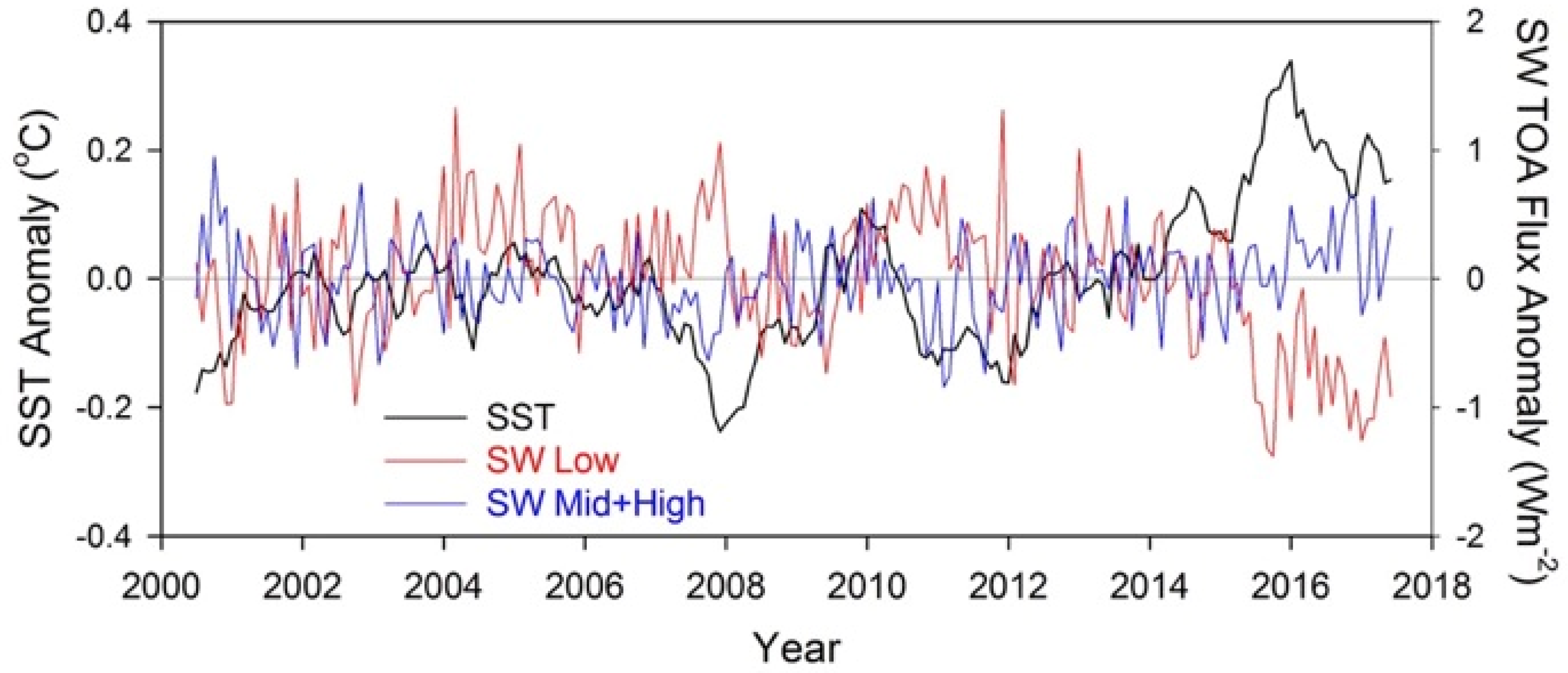
3.1. Global TOA Radiation Variation

During the CERES period, global mean surface air temperature anomalies (relative to 1951–1980) show a weak increase through the end of 2013, followed by a factor of 6 steeper increase from 2014 onwards (Figure 1a), marking the end of the global warming hiatus. In contrast, the cumulative planetary heat uptake derived from CERES global monthly mean net downward fluxes shows a continual increase with time (Figure 1b). Superimposed on this increase is an annual cycle that peaks in April and reaches a minimum in September. This occurs because global mean net TOA flux is positive between October–April and negative between May–September [43]. As a result, in a given year the cumulative heat uptake peaks in April and reaches its minimum in September. Since the planetary heat uptake accounts for the entire energy added to or removed from the climate system, it arguably provides a more fundamental measure of global warming than global mean surface temperature, which is influenced by other decadal processes internal to the climate at the air-sea interface [3,28,44].
For the entire available CERES period, the average rate of heat uptake is 0.67 Wm−2, and the standard deviations in annual and monthly anomalies are 0.33 Wm−2 and 0.69 Wm−2, respectively. The large variability is mainly due to El Niño–Southern Oscillation (ENSO) [14]. Figure 2a,b illustrate how global TOA flux anomalies in reflected SW, emitted LW and net downward radiation vary along with the Multivariate ENSO Index (MEI). We define SW and LW TOA fluxes as positive upwards and net TOA flux as positive downwards, following the convention used in the CERES data products. Appreciable positive SW and negative LW anomalies are observed at the beginning of the CERES record (Figure 2a), which coincides with a prolonged period of La Niña conditions that started in mid-1998 and ended in mid-2001. After 2002, SW and LW anomalies remain relatively weak until 2014, when SW anomalies sharply decrease and LW anomalies increase. The SW anomalies after 2014 are particularly noteworthy as they reach −2 Wm−2 in January 2017, one year after the peak of the 2015–2016 El Niño event. In contrast, the net TOA radiation anomalies (Figure 2b) are relatively small early in the record owing to cancellation between SW and LW anomalies, but become appreciable in the middle of the record when modest SW and LW TOA flux anomalies of the same sign combine (e.g., minima in 2002 and 2010, maxima in 2008 and 2012). After 2014, net TOA flux anomalies are generally positive due to the large negative anomalies in reflected SW, which overwhelms positive outgoing LW anomalies. The positive anomalies in net TOA flux following the 2015–2016 El Niño stand in marked contrast with those for the other El Niño events during the CERES period (2002–2003, 2004–2005, 2006–2007 and 2009–2010). Following those events, net TOA flux anomalies are generally negative.
In order to gain confidence that the TOA flux anomalies from EBAF Ed4.0 are robust, we compare them with TOA flux monthly anomalies from the SSF1deg Ed4.0 products for Terra, Aqua and S-NPP (Figure 3a–c). The EBAF Ed4.0 processing relies on CERES Terra measurements from March 2000-June 2002 and combined Terra and Aqua for July 2002–September 2017. EBAF Ed4.0 also supplements the CERES measurements with MODIS for scene information and geostationary imager measurements to capture variations in the diurnal cycle [31]. In contrast, the SSF1deg data product relies only on CERES and MODIS or VIIRS and is produced separately for each mission. As shown, there is excellent agreement between the different data products. All four datasets show a decline in SW anomalies and positive anomalies in LW TOA flux following the 2015–2016 El Niño. Root-mean-square (RMS) differences between EBAF Ed4.0 and the 3 SSF1deg records are <0.12 Wm−2 for SW, <0.16 Wm−2 for LW and <0.17 Wm−2 for net TOA flux (Table 2).
To further highlight how unprecedented the SW anomalies are during the last 3 years of the record (i.e., post-hiatus period), Figure 4a–c show lagged regressions between TOA flux anomalies and anomalies in the Niño 3.4 index for March 2000–June 2014 and for the entire CERES record (March 2000–September 2017). Consistent with other studies [4,45], Figure 4c shows that when TOA net radiation leads Niño 3.4 (negative lags), the regression slopes are positive for lags of up to 15 months. Conversely, when Niño 3.4 leads (positive lags), regression slopes are negative over the same period. Thus, a major El Niño occurring at zero lag would tend to be preceded within a year or so by an uptake of heat into the system and followed by a release of heat out of the system. This pattern is mainly driven by outgoing LW radiation (Figure 4b), which shows negative anomalies prior to an El Niño event and even stronger positive anomalies a few months following an El Niño, when surface temperatures are larger [46]. However, when the entire CERES record that includes the last 3 post-hiatus years is considered (red line), regression slopes for net and SW TOA flux (Figure 4a,c, respectively) fall outside of the 95% confidence intervals for positive lags. The unprecedented negative reflected SW anomalies following the 2015–2016 El Niño significantly alter the statistical TOA net radiation response following an El Niño event. Including this event reduces the amount of heat released out of the system following an El Niño relative to that expected based upon the first 14 years of the CERES record.

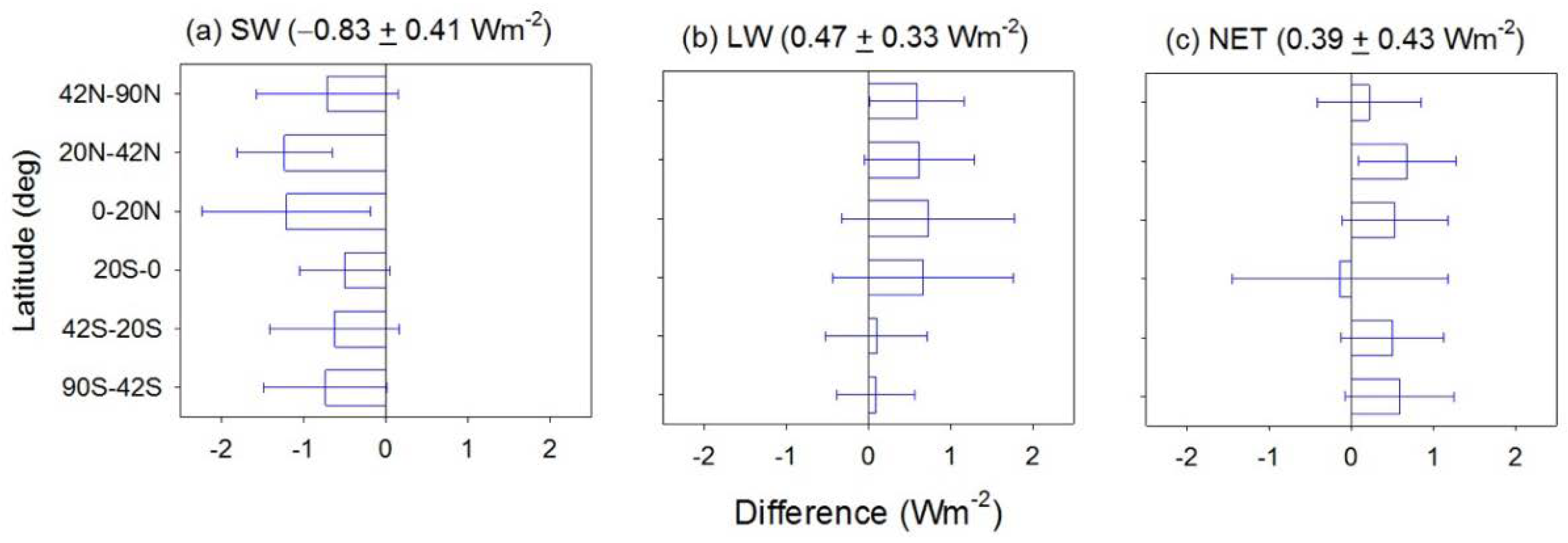
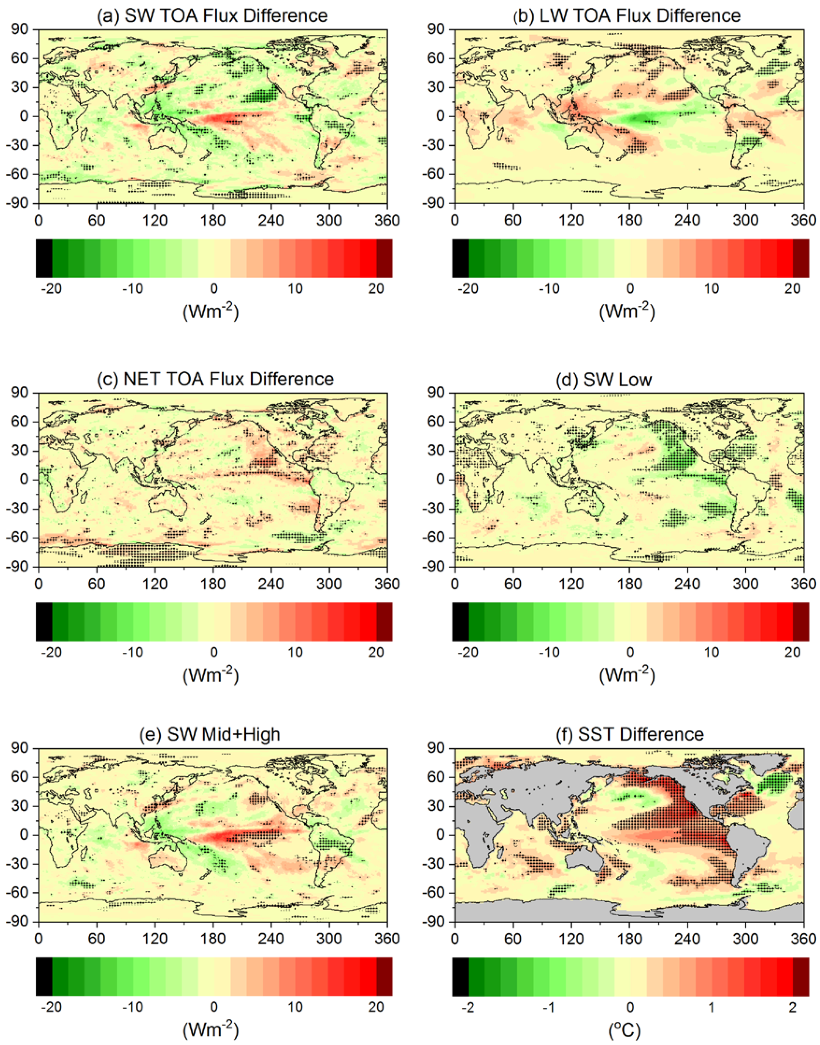
3.2. All-Sky TOA Flux Differences between Post-Hiatus and Hiatus Periods

Zonal mean TOA flux differences between the post-hiatus (July 2014–June 2017) and hiatus (July 2000–June 2014) periods are shown in Figure 5a–c. The six latitudes zones cover approximately the same area, so that each latitude zone contributes equal weight to the global mean. SW TOA flux mean differences are negative in each latitude zone, but exceed the 95% confidence interval only in the northern hemisphere (NH) tropics and subtropics. In contrast, LW TOA flux differences are positive in each latitude zone, but remain within the 95% confidence interval everywhere. Since the magnitudes of the differences are generally greater in the SW than LW, net TOA flux differences are positive in most latitude zones, except the southern hemisphere (SH) tropics. On a global average, mean differences between the post-hiatus and hiatus periods are: –0.83 ± 0.41 Wm−2, 0.47 ± 0.33 Wm−2 and 0.39 ± 0.43 Wm−2 for SW, LW and net, respectively. It is worth noting that the corresponding global mean solar irradiance difference is only 0.03 ± 0.13 Wm−2, and therefore has a negligible impact on radiation budget differences between these two periods.
Regionally, differences between the post-hiatus and hiatus periods are remarkable (Figure 6a–f). Figure 6a–c provide results for SW, LW and net TOA flux differences, while Figure 6d,e show contributions to SW TOA flux differences from low cloud fraction and combined middle and high cloud fraction changes, respectively, using the perturbation methodology described in Section 2. Large reductions in SW TOA flux are apparent off the west coasts of North and South America and over the northeastern Pacific, the west tropical Pacific, and the Southern Pacific Convergence Zone (Figure 6a). SW TOA flux differences off the coast of California are especially large, reaching 16 Wm−2. Because the decreases in reflected SW TOA flux occur in regions dominated by low cloud, the magnitude of the differences in LW TOA flux are smaller than for SW (Figure 6b). As a result, regional increases in net TOA flux are observed over large portions of the eastern Pacific off of North and South America (Figure 6c).
Figure 6d isolates the impact of low cloud cover on SW TOA flux differences using the partial radiative perturbation methodology. The correlation coefficient between global mean all-sky SW TOA flux anomalies and anomalies in SW TOA flux associated only with low cloud cover variations is 0.66 and the regression slope is 0.81 ± 0.13. The difference pattern for the low cloud cover contribution to SW TOA flux differences closely resembles the spatial pattern of SST differences (Figure 6f). Global mean SW TOA flux anomalies associated with low cloud cover changes are anti-correlated with SST anomalies (Figure 7), with a correlation coefficient of −0.48, and a regression slope of −2.3 ± 0.93 Wm−2 K−1. If only the hiatus period (July 2000–June 2014) is considered, the regression slope between SW TOA flux and SST anomalies is −0.37 ± 1.3 Wm−2 K−1. This marked change in the value of the regression slope between these two periods underscores the challenge involved with quantifying cloud feedback from interannual variability [47,48]. In order to reduce the uncertainty due to climate noise, a long observational record is needed [17,49]. Despite the difficulty in quantifying low cloud feedback with short observational records, the physical relationship between low cloud cover and SST is robust. On interannual timescales, marine stratocumulus cloud cover is correlated with lower-tropospheric stability [50,51]. An increase in local SST reduces the stability of the marine boundary layer (MBL), which leads to a deepening of the MBL, a decoupling between the cloud layer and its supply of surface moisture, and a reduction in cloud cover.
In order to explore the role of the unprecedented low cloud changes over the subtropical Pacific on regional climate off Baja California, Myers et al. [52] analyze the energy budget of the ocean mixed layer between January 2014 and September 2015. They find that surface radiation changes associated with the decrease in low cloud fraction contributed significantly to the extremely warm SSTs. Thus, the warmer SSTs led to reduced low cloud cover, which in turn led to increased SSTs through an increase in radiation to the surface. They conclude that this low cloud feedback was a key to producing a marine “heatwave” off Baja California. Further north, SSTs over the Pacific were affected more by anomalously low surface-to-atmosphere turbulent heat fluxes and increases in horizontal ocean heat transport and vertical mixing than by the decrease in low cloud fraction.
In the tropics, positive differences in SW TOA flux over the central Pacific are associated with an eastward shift in convection during the 2015/2016 El Niño (Figure 6e), which also reduces LW TOA flux (Figure 6b). Mayer et al. [53] note that even though SSTs were extreme, the tropical Pacific upper ocean gained heat owing to a reduction of the Indonesian Throughflow volume and heat transport of warm water from the Pacific to the Indian Ocean. This differs from the previous major El Niño in 1997/1998, in which there was appreciable upper ocean heat loss.
In contrast to the cloud and radiation changes over the north Pacific, changes over the north Atlantic south of Greenland exhibit increases in SW TOA flux and decreases in LW TOA flux. These changes are due to an increase in middle and high cloud cover (Figure 6d,e). The cloud changes are associated with strong negative anomalies in SST, popularly known as the “North Atlantic Cold Blob”, which first appeared in 2015 and is believed to be associated with a reduction in the Atlantic meridional overturning circulation [54].

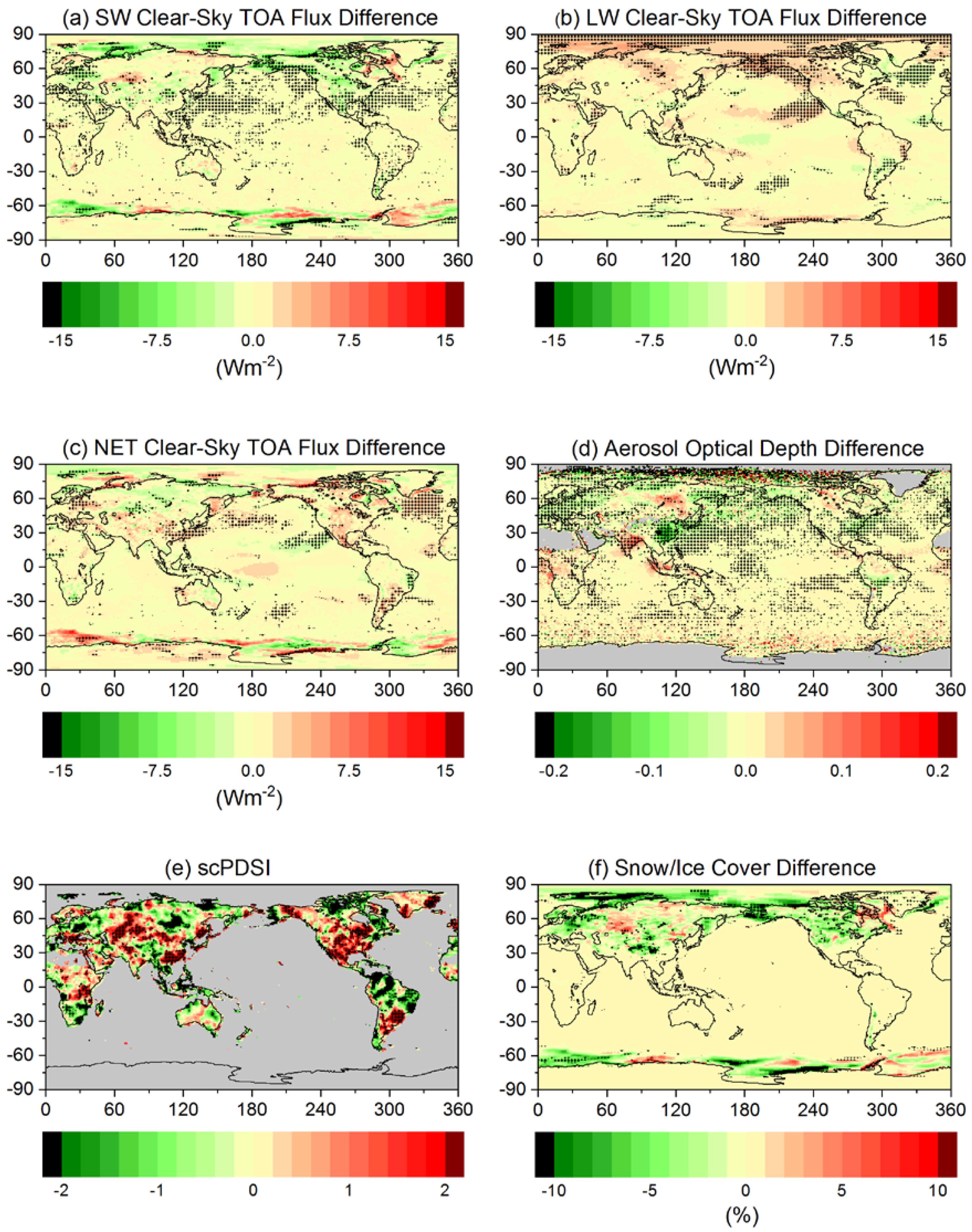
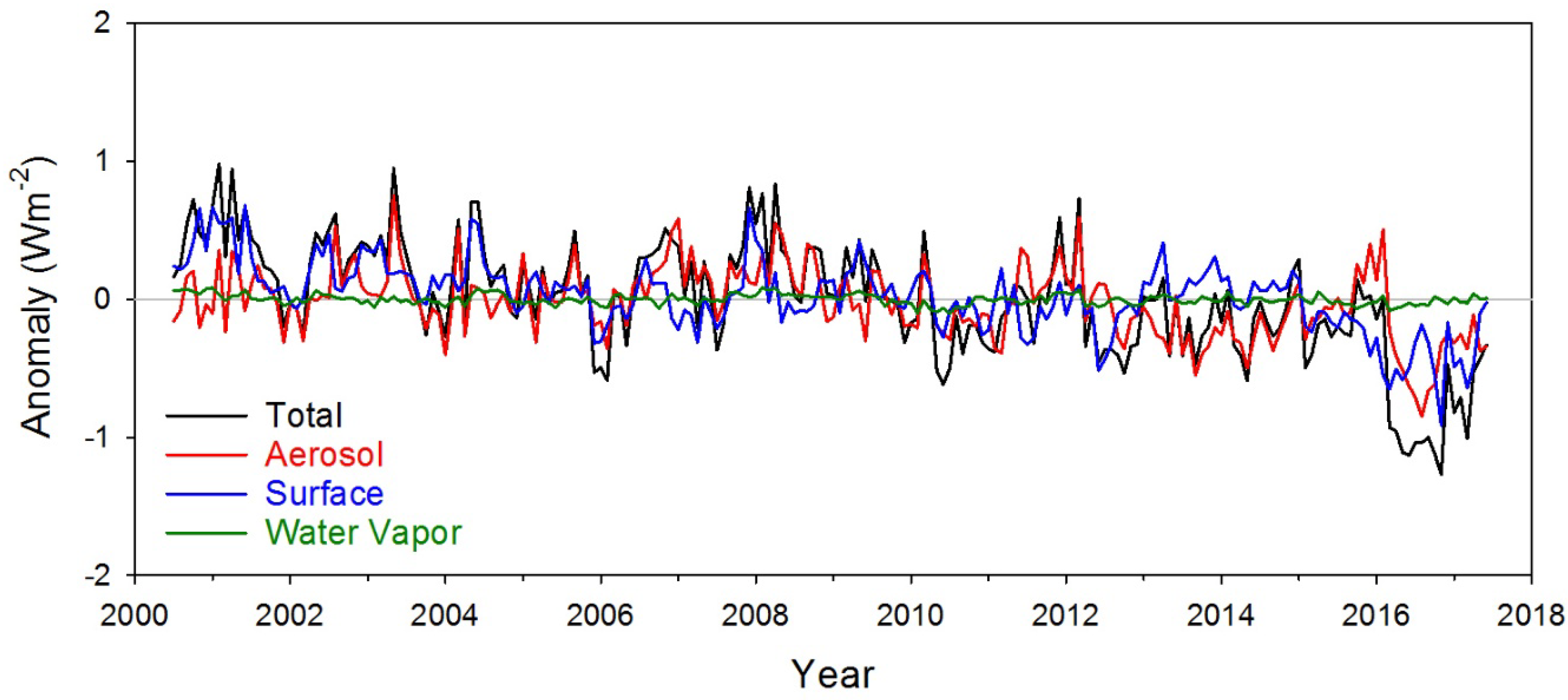
3.3. Clear-Sky TOA Flux Differences between Post-Hiatus and Hiatus Periods

Under clear-sky conditions, decreases in SW TOA flux are observed over the NH Pacific and Atlantic oceans, much of North America and over the Arctic (Figure 8a). The decreases in clear-sky SW TOA flux over ocean show a consistent pattern with decreases in MODIS AOD at 0.55 μm (Figure 8d). Importantly, the CERES EBAF clear-sky SW TOA fluxes are determined independently of MODIS AODs, so consistency in their regional patterns (particularly over ocean) suggests the differences are robust. While the SW TOA flux differences over ocean are only of order 1 Wm−2 and AOD differences are of order 0.03, they are significant at 95% confidence level in many regions. Zhao et al. [55] find similar decreases in AOD over east central China from MODIS and the Multi-angle Imaging SpectroRadiometer (MISR) through 2015. Using CERES EBAF Ed4.0 to infer clear-sky aerosol SW direct radiative effect, Paulot et al. [56] observe a decrease in aerosol radiative cooling over eastern China through 2015. Results in Figure 8a,b suggest that this trend continued after 2015. The large reductions in clear-sky SW TOA flux and AOD are associated with aggressive air-pollution control policies that were put in place in 2013 [57].
Reductions in SW TOA flux and AOD in the eastern US and subtropical Atlantic are also consistent with Zhao et al. [55], who find negative AOD trends of roughly −0.02 to −0.03 per decade from MODIS and MISR between 2001–2015. From data on emissions of major aerosol species, Zhao et al. [55] further find that the decrease in AOD is associated with reductions in all aerosol types except ammonia and dust. They note that the reductions are associated with implementation of control measures under the Clean Air Act [58]. Paulot et al. [56] find similar results and further note the dominant role of ongoing decreases in SO2 sources.
We applied the perturbation methodology to isolate the impact of various parameters on global mean clear-sky SW TOA flux (Figure 9). Not surprisingly, aerosol and surface albedo variations explain most of the SW TOA flux variability. Surface albedo changes are primarily from snow/ice changes (Figure 8f) over the Arctic and Southern Ocean adjacent to Antarctica. Similarly, negative differences in clear-sky SW TOA fluxes over western Canada and northern U.S. states are associated with decreases in snow cover. Over the central US and Mexico, SW TOA flux differences appear to correspond to differences in the self-calibrating Palmer Drought Severity Index (scPDSI) [42] (Figure 8e). As shown in Table 3, positive (negative) values of scPDSI indicate wetter (drier) soil conditions. Positive scPDSI differences over the western U.S. implies that wetter soil conditions occurred in more recent years compared to the first part of the century. Weiss et al. [59] note that both warmer temperatures and low precipitation were the cause for the greater soil moisture deficits. Since surface albedo tends to be lower in wetter surface soils [60], this likely is the reason for the lower SW TOA fluxes in these regions.
The regional pattern of LW clear-sky TOA flux differences between the post-hiatus and hiatus periods (Figure 8b) is similar to that for all-sky conditions (Figure 6b). Over the eastern Pacific, positive differences are associated with SST increases off of North and South America (Figure 6f). Reductions in clear-sky LW flux occur over the central equatorial Pacific where there is increased moisture owing to the eastward movement of convection during the 2015/2016 El Niño. Positive LW clear-sky differences occur throughout the Arctic region, reaching 5 Wm−2 over the northeast Kara Sea. Over the Atlantic, large decreases in clear-sky LW TOA flux occur over the North Atlantic Cold Blob, reaching −2.8 Wm−2. Differences in clear-sky net TOA flux (Figure 8c) are generally positive off the east coasts of China and North America owing to the decreases in SW TOA flux associated with reductions in AOD. Over the stratocumulus region off north America, net TOA flux decreases. The pattern is driven by increases in LW TOA flux that occur in response to the increased SSTs. In contrast to all-sky net TOA flux (Figure 6c), significant increases in clear-sky net TOA flux occur over the Atlantic Cold blob. On a global average, mean differences between the post-hiatus and hiatus periods are: –0.44 ± 0.39 Wm−2, 0.28 ± 0.32 Wm−2 and 0.19 ± 0.29 Wm−2 for clear-sky SW, LW and net, respectively. Zonal clear-sky TOA flux differences are particularly large between 20° N–42° N, reaching −0.83 ± 0.24 Wm−2 for SW and 0.57 ± 0.31 Wm−2 for net.

4. Temperature Tendency Difference between Post-Hiatus and Hiatus Periods

In order to place the results in this paper in the context of global mean temperature, we adopt a simple conceptual framework similar to Brown et al. [61] in which the TOA contribution to temperature change is determined separately from that due to vertical redistribution of heat through the bottom of the ocean’s mixed layer:
C m d T d t = Q T O A Q B M L
where d T d t is the temperature tendency, Q T O A is the TOA global mean net downward radiation, Q B M L is the heat across the bottom of the ocean’s mixed layer (positive downwards), and C m is the effective heat capacity of the climate system, given by
C m = 0.7 ρ C p D
where ρ is the density of sea water (1030 kg m−3), C p is the specific heat of water (4180 J kg−1 K−1), and D is the depth of the ocean’s mixed layer, assumed to be 75 m [61]. The 0.7 factor represents the ocean fraction. We calculate the temperature tendency separately for the hiatus and post-hiatus periods using GISTEMP [39] temperature anomalies. Q T O A is from CERES EBAF Ed4.0, expressed in terms of a monthly anomaly relative to climatology defined for 03/2000–09/2017. Q B M L is determined as a residual from Equation (3). Table 4 provides the results for the hiatus and post-hiatus periods. The results suggest that during the hiatus, the energy input from Q T O A only slightly exceeds the heat loss across the bottom of the mixed layer, resulting in a weak positive trend in T . In contrast, Q T O A increases by 65% following the hiatus, while Q B M L   decreases slightly, resulting in a marked increase in temperature tendency. Thus, this analysis suggests that the temperature trend difference between the hiatus and post-hiatus periods is primarily due to changes in Q T O A . This conclusion does not change when D is allowed to differ by 25 m between the hiatus and post-hiatus periods.

5. Summary and Conclusions

The aim of this study has been to examine what aspects of the Earth’s energy budget have changed and what components of the climate system caused those changes as we have come out of the so-called global warming hiatus between 1998–2013, in which the rate of global mean surface temperature slowed relative to the latter part of the 20th century. The analysis is limited to the CERES period after 2000, which covers most of the hiatus period and the first three years following the hiatus.
Global mean surface air temperatures show a weak increase between 2000 and 2013, followed by a factor of 6 steeper increase from 2014 onwards, which marks the end of the global warming hiatus. On the other hand the cumulative planetary heat uptake derived from CERES global monthly mean TOA net downward fluxes shows a continual increase with time throughout the CERES period. Superimposed on the long-term trend in planetary heat uptake is an annual cycle that arises because global mean net TOA flux is positive between October–April and negative between May–September. This variability is only apparent because CERES can resolve changes in net TOA flux down to monthly timescales. The change in planetary heat uptake arguably provides a better indication of how the climate system is changing than the rate of change in global mean surface temperature, which is strongly influenced by other factors at the air-sea interface.
During the CERES period, global mean outgoing SW and LW TOA flux anomalies remain relatively weak until 2014, when reflected SW anomalies sharply decrease and outgoing LW anomalies increase. The SW anomalies reach −2 Wm−2 in January 2017, one full year after the major El Niño event of 2015–2016. Net downward TOA flux anomalies after 2014 are generally positive due to the large decrease in reflected SW, which overwhelms the increase in outgoing LW radiation. Global mean SW TOA flux decreases by 0.83 ± 0.41 Wm−2 for July 2014–June 2017 (post-hiatus period) relative to July 2000–June 2014 (hiatus period), whereas for outgoing LW and net downward radiation the differences are 0.47 ± 0.33 Wm−2 and 0.39 ± 0.43 Wm−2, respectively. Following other El Niño events observed during the CERES record, increases in outgoing LW flux generally dominate over decreases in reflected SW flux, resulting in negative net TOA flux anomalies. TOA flux anomalies during the post-hiatus are thus highly unusual. To test the robustness of the results, we compared TOA flux anomalies from EBAF Ed4.0 with those produced separately for CERES instruments aboard Terra, Aqua and S-NPP. Anomalies from the different records were very close to one another with monthly RMS differences <0.2 Wm−2 and no apparent instrument drifts.
The decrease in global mean all-sky SW TOA flux between the post-hiatus and hiatus periods is primarily associated with areas over the eastern Pacific Ocean off North and South America, as well as over the west tropical Pacific and the Southern Pacific Convergence Zone. A partial radiative perturbation analysis reveals that decreases in low cloud cover are the primary driver of the SW TOA flux decreases. Furthermore, the regional distribution of decreases in SW TOA flux associated with low cloud cover changes closely matches that of SST warming, which in turn shows a pattern typical of the positive phase of the PDO over the eastern Pacific. In contrast to the decreases in SW TOA flux over the Pacific, increases occur over the north Atlantic associated with the North Atlantic Cold Blob, which partly compensates for the SW TOA flux decreases over the Pacific.
Changes in clear-sky TOA flux between the post-hiatus and hiatus periods also show distinct regional patterns. Post-hiatus SW TOA fluxes generally decrease relative to those during the hiatus period over the NH Pacific and Atlantic oceans, much of North America and over the Arctic. The SW TOA flux differences over ocean show a pattern consistent with changes in MODIS AODs, which are determined independently of CERES clear-sky SW TOA fluxes. Large reductions in clear-sky SW TOA flux and AOD east of China are consistent with aggressive air-pollution control policies that were put in place in 2013. Reductions in SW TOA flux and AOD in the eastern US and subtropical Atlantic are likely the result of the implementation of control measures under the Clean Air Act. Over the Arctic and NH extratropical land regions, marked decreases in SW TOA flux occur due to large reductions in sea-ice and snow cover.
In order to better understand the surface temperature changes during the post-hiatus and hiatus periods, we adopt a simple framework that relates surface temperature tendency with heating via TOA radiation and vertical redistribution of heat through the bottom of the ocean’s mixed layer. During the hiatus, the TOA energy input slightly exceeds the heat loss across the bottom of the ocean mixed layer, resulting in a weak positive trend in surface temperature. Following the hiatus, net radiation into the climate system increases by 65%, whereas heat loss through the bottom of the ocean mixed layer decreases slightly, resulting in a marked increase in temperature tendency. The results suggest that the temperature trend difference between the hiatus and post-hiatus periods is primarily due to TOA radiation changes particularly in the SW.

Author Contributions

Conceptualization, N.G.L., T.J.T. and J.R.N.; Methodology, N.G.L., T.J.T. and J.R.N.; Formal Analysis, N.G.L., T.J.T., H.W. and W.S.; Writing-Original Draft Preparation, N.G.L.; Writing-Review & Editing, N.G.L., T.J.T., J.R.N., H.W. and W.S.; Project Administration, N.G.L.

Funding

This research was supported by the NASA CERES project.

Acknowledgments

The NASA Langley Atmospheric Sciences Data Center processed the instantaneous Single Scanner Footprint (SSF) data used as input to EBAF Ed4.0.

Conflicts of Interest

The authors declare no conflict of interest.

References

  1. Rhein, M.A.; Rintoul, S.R.; Aoki, S.; Campos, E.; Chambers, D.; Feely, R.A.; Gulev, S.; Johnson, G.C.; Josey, S.A.; Kostianoy, A.; et al. Observations: Ocean. In Climate Change 2013: The Physical Science Basis; Stocker, T.F., Qin, D., Plattner, G.-K., Tignor, M., Allen, S.K., Boschung, J., Nauels, A., Xia, Y., Bex, V., Midgley, P.M., et al., Eds.; Contribution of Working Group I to the Fifth Assessment Report of the Intergovernmental Panel on Climate Change; Cambridge University Press: Cambridge, UK, 2013; pp. 255–315. [Google Scholar]
  2. Hansen, J.; Sato, M.; Kharecha, P.; von Schuckmann, K. Earth’s energy imbalance and implications. Atmos. Chem. Phys. 2011, 11, 13421–13449. [Google Scholar] [CrossRef] [Green Version]
  3. Von Schuckmann, K.; Palmer, M.D.; Trenberth, K.E.; Cazenave, A.; Chambers, D.; Champollion, N.; Hansen, J.; Josey, S.A.; Loeb, N.; Mathieu, P.-P.; et al. An imperative to monitor Earth’s energy imbalance. Nat. Clim. Chang. 2016, 6, 138–144. [Google Scholar] [CrossRef] [Green Version]
  4. Xie, S.-P.; Kosaka, Y.; Okumura, Y.M. Distinct energy budgets for anthropogenic and natural changes during global warming hiatus. Nat. Geosci. 2016, 9, 29–33. [Google Scholar] [CrossRef]
  5. Hansen, J. Earth’s Energy Imbalance: Confirmation and Implications. Science 2005, 308, 1431–1435. [Google Scholar] [CrossRef] [PubMed]
  6. Collins, M.; Knutti, R.; Arblaster, J.; Dufresne, J.L.; Fichefet, T.; Friedlingstein, P.; Gao, X.; Gutowski, W.J.; Johns, T.; Krinner, G.; et al. Long-term Climate Change: Projections, Commitments and Irreversibility. In Climate Change 2013: The Physical Science Basis; Stocker, T.F., Qin, D., Plattner, G.-K., Tignor, M., Allen, S.K., Boschung, J., Nauels, A., Xia, Y., Bex, V., Midgley, P.M., et al., Eds.; Contribution of Working Group I to the Fifth Assessment Report of the Intergovernmental Panel on Climate Change; Cambridge University Press: Cambridge, UK, 2013; pp. 1029–1136. [Google Scholar]
  7. Palmer, M.D.; McNeall, D.J.; Dunstone, N.J. Importance of the deep ocean for estimating decadal changes in Earth’s radiation balance: Importance of Deep Ocean. Geophys. Res. Lett. 2011, 38, 1–5. [Google Scholar] [CrossRef]
  8. Yan, X.-H.; Boyer, T.; Trenberth, K.; Karl, T.R.; Xie, S.-P.; Nieves, V.; Tung, K.-K.; Roemmich, D. The global warming hiatus: Slowdown or redistribution?: The Global Warming Hiatus. Earths Future 2016, 4, 472–482. [Google Scholar] [CrossRef]
  9. Trenberth, K.E. Has there been a hiatus? Science 2015, 349, 691–692. [Google Scholar] [CrossRef] [PubMed] [Green Version]
  10. Hartmann, D.L.; Tank, A.M.; Rusticucci, M.; Alexander, L.V.; Brönnimann, S.; Charabi, Y.A.; Dentener, F.J.; Dlugokencky, E.J.; Easterling, D.R.; Kaplan, A.; et al. Observations: Atmosphere and Surface. In Climate Change 2013: The Physical Science Basis; Stocker, T.F., Qin, D., Plattner, G.-K., Tignor, M., Allen, S.K., Boschung, J., Nauels, A., Xia, Y., Bex, V., Midgley, P.M., et al., Eds.; Contribution of Working Group I to the Fifth Assessment Report of the Intergovernmental Panel on Climate Change; Cambridge University Press: Cambridge, UK, 2013; pp. 159–254. [Google Scholar]
  11. Balmaseda, M.A.; Trenberth, K.E.; Källén, E. Distinctive climate signals in reanalysis of global ocean heat content: Signals in Ocean Heat Content. Geophys. Res. Lett. 2013, 40, 1754–1759. [Google Scholar] [CrossRef]
  12. Meehl, G.A.; Hu, A.; Arblaster, J.M.; Fasullo, J.; Trenberth, K.E. Externally Forced and Internally Generated Decadal Climate Variability Associated with the Interdecadal Pacific Oscillation. J. Clim. 2013, 26, 7298–7310. [Google Scholar] [CrossRef] [Green Version]
  13. England, M.H.; McGregor, S.; Spence, P.; Meehl, G.A.; Timmermann, A.; Cai, W.; Gupta, A.S.; McPhaden, M.J.; Purich, A.; Santoso, A. Recent intensification of wind-driven circulation in the Pacific and the ongoing warming hiatus. Nat. Clim. Chang. 2014, 4, 222–227. [Google Scholar] [CrossRef] [Green Version]
  14. Trenberth, K.E.; Fasullo, J.T.; Balmaseda, M.A. Earth’s Energy Imbalance. J. Clim. 2014, 27, 3129–3144. [Google Scholar] [CrossRef]
  15. Santer, B.D.; Bonfils, C.; Painter, J.F.; Zelinka, M.D.; Mears, C.; Solomon, S.; Schmidt, G.A.; Fyfe, J.C.; Cole, J.N.S.; Nazarenko, L.; et al. Volcanic contribution to decadal changes in tropospheric temperature. Nat. Geosci. 2014, 7, 185–189. [Google Scholar] [CrossRef] [Green Version]
  16. Solomon, S.; Daniel, J.S.; Neely, R.R.; Vernier, J.-P.; Dutton, E.G.; Thomason, L.W. The Persistently Variable “Background” Stratospheric Aerosol Layer and Global Climate Change. Science 2011, 333, 866–870. [Google Scholar] [CrossRef] [PubMed]
  17. Zhou, C.; Zelinka, M.D.; Klein, S.A. Impact of decadal cloud variations on the Earth’s energy budget. Nat. Geosci. 2016, 9, 871–874. [Google Scholar] [CrossRef]
  18. Bond, N.A.; Cronin, M.F.; Freeland, H.; Mantua, N. Causes and impacts of the 2014 warm anomaly in the NE Pacific: 2014 Warm Anomaly in the NE Pacific. Geophys. Res. Lett. 2015, 42, 3414–3420. [Google Scholar] [CrossRef]
  19. Huang, B.; Thorne, P.W.; Banzon, V.F.; Boyer, T.; Chepurin, G.; Lawrimore, J.H.; Menne, M.J.; Smith, T.M.; Vose, R.S.; Zhang, H.-M. Extended Reconstructed Sea Surface Temperature, Version 5 (ERSSTv5): Upgrades, Validations, and Intercomparisons. J. Clim. 2017, 30, 8179–8205. [Google Scholar] [CrossRef] [Green Version]
  20. Tseng, Y.-H.; Ding, R.; Huang, X. The warm Blob in the northeast Pacific—The bridge leading to the 2015/16 El Niño. Environ. Res. Lett. 2017, 12, 054019. [Google Scholar] [CrossRef]
  21. Allan, R.P.; Liu, C.; Loeb, N.G.; Palmer, M.D.; Roberts, M.; Smith, D.; Vidale, P.-L. Changes in global net radiative imbalance 1985–2012. Geophys. Res. Lett. 2014, 41, 5588–5597. [Google Scholar] [CrossRef] [PubMed]
  22. Loeb, N.G.; Lyman, J.M.; Johnson, G.C.; Allan, R.P.; Doelling, D.R.; Wong, T.; Soden, B.J.; Stephens, G.L. Observed changes in top-of-the-atmosphere radiation and upper-ocean heating consistent within uncertainty. Nat. Geosci. 2012, 5, 110–113. [Google Scholar] [CrossRef]
  23. Johnson, G.C.; Lyman, J.M.; Loeb, N.G. Improving estimates of Earth’s energy imbalance. Nat. Clim. Chang. 2016, 6, 639–640. [Google Scholar] [CrossRef]
  24. Wong, T.; Wielicki, B.A.; Lee, R.B.; Smith, G.L.; Bush, K.A.; Willis, J.K. Reexamination of the Observed Decadal Variability of the Earth Radiation Budget Using Altitude-Corrected ERBE/ERBS Nonscanner WFOV Data. J. Clim. 2006, 19, 4028–4040. [Google Scholar] [CrossRef] [Green Version]
  25. Lyman, J.M.; Good, S.A.; Gouretski, V.V.; Ishii, M.; Johnson, G.C.; Palmer, M.D.; Smith, D.M.; Willis, J.K. Robust warming of the global upper ocean. Nature 2010, 465, 334–337. [Google Scholar] [CrossRef] [PubMed]
  26. Abraham, J.P.; Baringer, M.; Bindoff, N.L.; Boyer, T.; Cheng, L.J.; Church, J.A.; Conroy, J.L.; Domingues, C.M.; Fasullo, J.T.; Gilson, J.; et al. A review of global ocean temperature observations: Implications for ocean heat content estimates and climate change: Review of Ocean Observations. Rev. Geophys. 2013, 51, 450–483. [Google Scholar] [CrossRef]
  27. Smith, D.M.; Allan, R.P.; Coward, A.C.; Eade, R.; Hyder, P.; Liu, C.; Loeb, N.G.; Palmer, M.D.; Roberts, C.D.; Scaife, A.A. Earth’s energy imbalance since 1960 in observations and CMIP5 models: Earth’s energy imbalance since 1960. Geophys. Res. Lett. 2015, 42, 1205–1213. [Google Scholar] [CrossRef] [PubMed]
  28. Roemmich, D.; Church, J.; Gilson, J.; Monselesan, D.; Sutton, P.; Wijffels, S. Unabated planetary warming and its ocean structure since 2006. Nat. Clim. Chang. 2015, 5, 240–245. [Google Scholar] [CrossRef]
  29. Lewandowsky, S.; Risbey, J.S.; Oreskes, N. On the definition and identifiability of the alleged “hiatus” in global warming. Sci. Rep. 2015, 5, 16784. [Google Scholar] [CrossRef] [PubMed] [Green Version]
  30. Zhang, Y.; Wallace, J.M.; Battisti, D.S. ENSO-like interdecadal variability: 1900–93. J. Clim. 1997, 10, 1004–1020. [Google Scholar] [CrossRef]
  31. Loeb, N.G.; Doelling, D.R.; Wang, H.; Su, W.; Nguyen, C.; Corbett, J.G.; Liang, L.; Mitrescu, C.; Rose, F.G.; Kato, S. Clouds and the Earth’s Radiant Energy System (CERES) Energy Balanced and Filled (EBAF) Top-of-Atmosphere (TOA) Edition-4.0 Data Product. J. Clim. 2018, 31, 895–918. [Google Scholar] [CrossRef]
  32. Levy, R.C.; Mattoo, S.; Munchak, L.A.; Remer, L.A.; Sayer, A.M.; Patadia, F.; Hsu, N.C. The Collection 6 MODIS aerosol products over land and ocean. Atmos. Meas. Tech. 2013, 6, 2989–3034. [Google Scholar] [CrossRef] [Green Version]
  33. Wetherald, R.T.; Manabe, S. Cloud Feedback Processes in a General Circulation Model. J. Atmos. Sci. 1988, 45, 1397–1415. [Google Scholar] [CrossRef]
  34. Thorsen, T.J.; Kato, S.; Loeb, N.G.; Rose, F.G. Observation-based decomposition of radiative perturbations and radiative kernels. J. Clim. 2018, in press. [Google Scholar]
  35. Rose, F.G.; Rutan, D.A.; Charlock, T.; Smith, G.L.; Kato, S. An Algorithm for the Constraining of Radiative Transfer Calculations to CERES-Observed Broadband Top-of-Atmosphere Irradiance. J. Atmos. Ocean. Technol. 2013, 30, 1091–1106. [Google Scholar] [CrossRef]
  36. Rienecker, M.M.; Suarez, M.J.; Gelaro, R.; Todling, R.; Bacmeister, J.; Liu, E.; Bosilovich, M.G.; Schubert, S.D.; Takacs, L.; Kim, G.-K.; et al. MERRA: NASA’s Modern-Era Retrospective Analysis for Research and Applications. J. Clim. 2011, 24, 3624–3648. [Google Scholar] [CrossRef]
  37. Collins, W.D.; Rasch, P.J.; Eaton, B.E.; Khattatov, B.V.; Lamarque, J.-F.; Zender, C.S. Simulating aerosols using a chemical transport model with assimilation of satellite aerosol retrievals: Methodology for INDOEX. J. Geophys. Res. Atmos. 2001, 106, 7313–7336. [Google Scholar] [CrossRef] [Green Version]
  38. Doelling, D.R.; Loeb, N.G.; Keyes, D.F.; Nordeen, M.L.; Morstad, D.; Nguyen, C.; Wielicki, B.A.; Young, D.F.; Sun, M. Geostationary Enhanced Temporal Interpolation for CERES Flux Products. J. Atmos. Ocean. Technol. 2013, 30, 1072–1090. [Google Scholar] [CrossRef]
  39. Hansen, J.; Ruedy, R.; Sato, M.; Lo, K. Global Surface Temperature Change. Rev. Geophys. 2010, 48. [Google Scholar] [CrossRef]
  40. Wolter, K.; Timlin, M.S. Measuring the strength of ENSO events: How does 1997/1998 rank? Weather 1998, 53, 315–324. [Google Scholar] [CrossRef]
  41. Brodzik, M.J.; Stewart, J.S. Near-Real-Time SSM/I-SSMIS EASE-Grid Daily Global Ice Concentration and Snow Extent; Version 5; NASA National Snow and Ice Data Center Distributed Active Archive Center: Boulder, CO, USA, 2016. [Google Scholar]
  42. Van der Schrier, G.; Barichivich, J.; Briffa, K.R.; Jones, P.D. A scPDSI-based global data set of dry and wet spells for 1901–2009: Variations in the Self-Calibrating PDSI. J. Geophys. Res. Atmos. 2013, 118, 4025–4048. [Google Scholar] [CrossRef]
  43. Fasullo, J.T.; Trenberth, K.E. The Annual Cycle of the Energy Budget. Part I: Global Mean and Land–Ocean Exchanges. J. Clim. 2008, 21, 2297–2312. [Google Scholar] [CrossRef] [Green Version]
  44. Victor, D.G.; Kennel, C.F. Ditch the 2 °C warming goal. Nature 2014, 514, 30–31. [Google Scholar] [CrossRef] [PubMed]
  45. Brown, P.T.; Li, W.; Jiang, J.H.; Su, H. Unforced Surface Air Temperature Variability and Its Contrasting Relationship with the Anomalous TOA Energy Flux at Local and Global Spatial Scales. J. Clim. 2016, 29, 925–940. [Google Scholar] [CrossRef]
  46. Trenberth, K.E.; Caron, J.M.; Stepaniak, D.P.; Worley, S. Evolution of El Niño–Southern Oscillation and global atmospheric surface temperatures. J. Geophys. Res. 2002, 107. [Google Scholar] [CrossRef] [Green Version]
  47. Forster, P.M. Inference of Climate Sensitivity from Analysis of Earth’s Energy Budget. Annu. Rev. Earth Planet. Sci. 2016, 44, 85–106. [Google Scholar] [CrossRef]
  48. Loeb, N.G.; Su, W.; Kato, S. Understanding Climate Feedbacks and Sensitivity Using Observations of Earth’s Energy Budget. Curr. Clim. Chang. Rep. 2016, 2, 170–178. [Google Scholar] [CrossRef]
  49. Chung, E.-S.; Soden, B.J.; Clement, A.C. Diagnosing Climate Feedbacks in Coupled Ocean–Atmosphere Models. Surv. Geophys. 2012, 33, 733–744. [Google Scholar] [CrossRef]
  50. Klein, S.A.; Hartmann, D.L.; Norris, J.R. On the relationship among low-cloud structure, sea surface temperature, and atmospheric circulation in the summertime Northeast Pacific. J. Clim. 1995, 8, 1140–1155. [Google Scholar] [CrossRef]
  51. Wood, R. Stratocumulus Clouds. Mon. Weather Rev. 2012, 140, 2373–2423. [Google Scholar] [CrossRef]
  52. Myers, T.A.; Mechoso, C.R.; Cesana, G.V.; DeFlorio, M.J.; Waliser, D.E. Cloud Feedback Key to Marine Heatwave off Baja California. Geophys. Res. Lett. 2018, 45, 4345–4352. [Google Scholar] [CrossRef]
  53. Mayer, M.; Alonso Balmaseda, M.; Haimberger, L. Unprecedented 2015/2016 Indo-Pacific Heat Transfer Speeds Up Tropical Pacific Heat Recharge. Geophys. Res. Lett. 2018, 45, 3274–3284. [Google Scholar] [CrossRef] [PubMed]
  54. Josey, S.A.; Hirschi, J.J.-M.; Sinha, B.; Duchez, A.; Grist, J.P.; Marsh, R. The recent atlantic cold anomaly: Causes, consequences, and related phenomena. Annu. Rev. Mar. Sci. 2017, 10, 475–501. [Google Scholar] [CrossRef] [PubMed]
  55. Zhao, B.; Jiang, J.H.; Gu, Y.; Diner, D.; Worden, J.; Liou, K.-N.; Su, H.; Xing, J.; Garay, M.; Huang, L. Decadal-scale trends in regional aerosol particle properties and their linkage to emission changes. Environ. Res. Lett. 2017, 12, 054021. [Google Scholar] [CrossRef] [Green Version]
  56. Paulot, F.; Paynter, D.; Ginoux, P.; Naik, V.; Horowitz, L. Changes in the aerosol direct radiative forcing from 2001 to 2015: Observational constraints and regional mechanisms. Atmos. Chem. Phys. 2018. [Google Scholar] [CrossRef]
  57. Jin, Y.; Andersson, H.; Zhang, S. Air Pollution Control Policies in China: A Retrospective and Prospects. Int. J. Environ. Res. Public Health 2016, 13, 1219. [Google Scholar] [CrossRef] [PubMed]
  58. Xing, J.; Pleim, J.; Mathur, R.; Pouliot, G.; Hogrefe, C.; Gan, C.-M.; Wei, C. Historical gaseous and primary aerosol emissions in the United States from 1990 to 2010. Atmos. Chem. Phys. 2013, 13, 7531–7549. [Google Scholar] [CrossRef]
  59. Weiss, J.L.; Castro, C.L.; Overpeck, J.T. Distinguishing Pronounced Droughts in the Southwestern United States: Seasonality and Effects of Warmer Temperatures. J. Clim. 2009, 22, 5918–5932. [Google Scholar] [CrossRef]
  60. Idso, S.B.; Jackson, R.D.; Kimball, B.A.; Nakayama, F.S. The Dependence of Bare Soil Albedo on Soil Water Content. J. Appl. Meteorol. Climatol. 1975, 14, 109–113. [Google Scholar] [CrossRef] [Green Version]
  61. Brown, P.T.; Li, W.; Li, L.; Ming, Y. Top-of-atmosphere radiative contribution to unforced decadal global temperature variability in climate models. Geophys. Res. Lett. 2014, 41, 5175–5183. [Google Scholar] [CrossRef] [Green Version]
Figure 1. (a) National Aeronautics and Space Administration Goddard Institute for Space Studies Surface Temperature Analysis (GISTEMP) global mean surface air temperature anomaly relative to 1951–1980 climatology and (b) Clouds and the Earth’s Radiant Energy System (CERES) cumulative planetary heat uptake for March 2000–September 2017.
Climate 06 00062 g001
Figure 2. Global mean (a) shortwave (SW) and longwave (LW) and (b) net top-of-atmosphere (TOA) flux anomalies for March 2000–September 2017 from CERES Energy Balanced and Filled (EBAF) Ed4.0. Thin lines denote monthly anomalies, thick lines are 12-month running means. Vertical black bars show the Multivariate ENSO Index (MEI). Anomalies are calculated relative to climatology over the entire period. SW and LW TOA flux anomalies are defined as positive upwards and net TOA flux anomalies are positive downwards.
Climate 06 00062 g002
Figure 3. Deseasonalized monthly anomalies in global mean (a) SW, (b) LW and (c) net TOA radiation from EBAF Ed4.0, SSF1deg-Ed4.0 Terra (TER), Aqua (AQU) and Suomi-NPP (SNPP). Anomalies are calculated using a common climatology from February 2012–June 2017.
Climate 06 00062 g003
Figure 4. Lagged regression of (a) reflected SW, (b) outgoing LW and (c) net TOA flux anomalies against anomalies in T3.4 for March 2000–June 2014 and March 2000–September 2017. Positive lags indicate that T3.4 leads. Blue shaded areas correspond to 95% confidence interval in regression slopes.
Climate 06 00062 g004
Figure 5. Zonal mean differences in TOA (a) reflected SW, (b) outgoing LW and (c) net TOA flux for the post-hiatus (July 2014–June 2017) minus hiatus (July 2000–June 2014) periods. Error bars correspond to 95% confidence intervals in the mean differences.
Climate 06 00062 g005
Figure 6. Regional distribution of mean difference between the post-hiatus (July 2014–June 2017) and hiatus (July 2000–June 2014) periods: (a) reflected SW, (b) outgoing LW, and (c) net TOA flux; (d) TOA SW flux low cloud contribution (SW Low), (e) TOA SW flux middle and high cloud contribution (SW Mid + High), (f) SST. Stippling denotes regions in which difference exceeds 95% confidence interval.
Climate 06 00062 g006
Figure 7. Anomalies in global mean SST and cloud fraction contributions to SW TOA flux from low clouds and mid + high clouds for July 2000–June 2017.
Climate 06 00062 g007
Figure 8. Regional distribution of mean difference between the post-hiatus (July 2014–June 2017) and hiatus (July 2000–June 2014) periods: (a) clear-sky reflected SW, (b) clear-sky outgoing LW, and (c) clear-sky net TOA flux; (d) 0.55 μm MODIS aerosol optical depth (AOD); (e) self-calibrating Palmer Drought Severity Index (scPDSI); (f) Snow/ice cover. Note that for AOD difference, hiatus period is July 2002–June 2014.
Climate 06 00062 g008
Figure 9. Anomalies in global mean contributions to clear-sky SW TOA flux from aerosols, surface albedo and water vapor.
Climate 06 00062 g009
Table 1. List of data products considered in this study.
ParameterData ProductTemporal RangeReference
TOA FluxCERES EBAF Ed4.0
CERES SSF1deg
March 2000–September 2017[31]
Cloud Properties and Surface AlbedoCERES SYN1deg Ed4.0March 2000–September 2017[38]
Surface TemperatureGISTEMPFebruary 2000–September 2017[39]
SST and Niño 3.4 IndexExtended Reconstructed Sea Surface
Temperature (ERSST) v5 averages
July 2000–June 2017[19]
MEIESRL MEIJanuary 1998–September 2017[40]
0.55 μm AODMYD04 Collection 6July 2002–June 2017[32]
Snow & Ice CoverNear-Real-Time SSM/I-SSMIS EASE-Grid Daily
Global Ice Concentration and Snow Extent
July 2000–June 2017[41]
Drought IndexSelf-calibrating Palmer Drought Severity Index (scPDSI)July 2000–June 2014[42]
Table 2. Root-mean-square (RMS) differences between monthly anomalies for different pairs of records used in Figure 3.
TERAQUSNPP
SWEBAF0.120.110.12
TER-0.190.19
AQU -0.083
LWEBAF0.160.0920.13
TER-0.190.13
AQU -0.16
NETEBAF0.150.150.17
TER-0.260.22
AQU -0.18
Table 3. Classification of the scPDSI.
scPDSIClass
>4.0extremely wet
3.0:4.0severely wet
2.0:3.0moderately wet
1.0:2.0slightly wet
0.5:1.0incipient wet spell
−0.5:0.5near normal
−0.5:−1.0incipient dry spell
−1.0:−2.0slightly dry
−2.0:−3.0moderately dry
−3.0:−4.0severely dry
<−4.0extremely dry
Table 4. Energy budget terms corresponding to Equation (3). Also shown are absorbed solar radiation (ASR) and outgoing longwave radiation (OLR) defined as positive downwards. Radiative quantities are anomalies relative to a climatology defined for March 2000–September 2017.
d T d t C m d T d t Q T O A Q B M L ASR−OLR
Hiatus0.00840.0600.6120.5520.5270.085
Post-Hiatus0.07320.5251.0070.4821.391−0.384
Difference0.0650.4640.395−0.0700.864−0.469

