The Hiatus in Global Warming and Interactions between the El Niño and the Pacific Decadal Oscillation: Comparing Observations and Modeling Results

1
OsloMet, Oslo Metropolitan University, Pilestredet 35 N, 0130 Oslo, Norway
2
NOAA/NWS/NCEP/Climate Prediction Center, 5830 University Research Court, NCWCP, College Park, MD 20740, USA
*
Author to whom correspondence should be addressed.
Climate 2018, 6(3), 72; https://0-doi-org.brum.beds.ac.uk/10.3390/cli6030072
Submission received: 9 July 2018
/
Revised: 24 August 2018
/
Accepted: 28 August 2018
/
Published: 4 September 2018
(This article belongs to the Special Issue Postmortem of the Global Warming Hiatus)
Abstract
:Ocean oscillations interact across large regions and these interactions may explain cycles in global temperature anomaly, including hiatus periods. Here, we examine ocean interaction measures and compare results from model simulations to observations for El Niño and the Pacific decadal oscillation (PDO). We use the global climate model of the Met Office Hadley Centre. A relatively novel method for identifying running leading-agging LL-relations show that the observed El Niño generally leads the observed PDO and this pattern is strengthened in the simulations. However, LL-pattern in both observations and models shows that there are three periods, around 1910–1920, around 1960 and around 2000 where El Niño lags PDO, or the leading signature is weak. These periods correspond to hiatus periods in global warming. The power spectral density analysis, (PSD), identifies various ocean cycle lengths in El Niño and PDO, but the LL-algorithm picks out common cycles of 7–8 and 24 years that shows leading-lagging relations between them.
1. Introduction
To study the effects of global warming on the global climate system, global circulation models are frequently used. The models are presently often fully coupled atmosphere, ocean, land and sea ice models. An overview of the models used in global warming studies can be found in Wang et al. [1] The model produces time series of ocean variables that describe climate models in the oceans, like the Niño index and the Pacific decadal oscillation, (PDO). Between pairs of movements there will be “bridges” that make one movement impact another. The “bridges” may be facilitated by surface or subsurface water flows, or by interactions with the atmosphere. In the ocean movement time series there will be patterns that reflect the impact of one movement on the other. Movements of ocean water appear to produce cycles in global warming, and of particular interest are the hiatus periods and the temperature “regime shifts”.
In the present study, we compare measures for interactions in the model and in observations. The comparison will express how the model manages to reproduce interactions in the observed system. However, discrepancies will give clues for how to improve the model. Secondly, since interactions probably reflect characteristics of the single series that are part of the interactions, we identify those characteristics of the single series that also show up in the interaction pattern. Thirdly, we examine how interactions between water movements influence global warming.
The modeled data in this study is from model HadGEM2-ES, a coupled Earth System Model developed at the Met Office Hadley Centre and used for the Coupled Model Intercomparison Project Phase 5 (CMIP5) simulations [2]. External forcing, such as anthropogenic CO2 emissions and other greenhouse gases, volcanic aerosol, etc., drives the model.
The broad rationale for applying techniques other than ordinary least squares (OLS) for comparing observations and modeling results is that interaction patterns, like leading or lagging (LL)-relations between paired series, their common cycles and their phase shifts may be important, but not easily quantified by the OLS technique. This is in particular true if the LL-relations change over short intervals. Secondly, there may be individual events and aggregated patterns in both the observed and the simulated system that are important for understanding the studied system. By designing tests that compare observed interactions with corresponding model interactions, causal mechanisms in models can be applied to interpretations of the real system with greater confidence.
Physical mechanisms that govern El Niño, PDO and other ocean variability or their proxies are not the issue here. However, in some cases, physical evidence from other studies may support patterns found with the techniques used here, and thus enhance the belief that similarities or differences between observed and modeled results are real and not the result of stochastic effects.
Paired series. Variables that describe interactions between ocean currents, pressure differences and land and atmospheric characteristics will typically show cyclic behavior. Since pairs of variables, like El Niño and the PDO are retrieved from ocean regions that overlap or are linked to each other through atmospheric or oceanic teleconnections, they may show common characteristics that can be captured partly with ordinary linear regression. For paired series, we therefore (A) examine if the regressions between observed pair of variables are similar to the regressions between the simulated versions of the same paired variables. However, observed and simulated series may be shifted relative to each other in time. (B) We capture such shifts by identifying leading-lagging (LL) relations, either for the whole series, or for portions of the series. In the latter case, we also report years when the LL-relations shift and compare these years to tie-points, e.g., years with changes in polarity for ocean variables reported in the literature [3,4]. (C) If the shifts are being leading or lagging they show cyclic characteristics. We then identify the cycles with the power spectral density (PSD) algorithm applied to the series that express the shifts. The cycles identified in this way characterize an aggregate property of the LL-relations. (D) We examine if cycles in the LL-relations have counterparts in cycles in the single series. We also identify (E) common cycle length and (F) phase shifts between cycles for the paired series.
The rest of the paper is organized as follows: Section 2 describes the material used in the study. In Section 3 we describe the methods used, particularly the leading-lagging LL-method where some novel technique has been added. The results are described in Section 4 and discussed in Section 5. Conclusions are given in Section 6.
2. Materials
The material consists of two parts: the time series for ocean current proxies and the “regime shifts” or “tie” points [5] during the period from 1861 to 2005 identified in the literature. We use the hiatus periods and the tie points identified in the literature to estimate whether the model results capture important events during the period.
We examine two variables that are closely related to the climate variability of the Pacific Ocean and/or global warming, and examine the interactions between these two variables. They are the El Niño and the PDO. Carbon dioxide (CO2) emissions are observed values that are used as a driving force for the model, as well as volcanic eruptions [6]. The global-mean temperature anomaly (GTA) is used in the literature to identify particular events, like hiatus periods and “tie” points in the global temperature change history.
The Niño 3.4 index is the average of sea surface temperature (SST) anomalies in the Niño 3.4 region (120° W–170° W, 5° S–5° N), with the unit of K (or °C). The index has been widely used to represent the variability of the El Niño-Southern Oscillation (ENSO), a major interannual climate mode in the tropics. We use annual data from 1861 to 2005 for this variable, that is 145 years of data. The values for the ENSO and tropical Pacific SST data set have a greater reliability after 1950 [1].
The Pacific decadal oscillation (PDO) is closely related to the interdecadal Pacific oscillation (IPO), but has a more northern hemisphere focus [7,8]. PDO is measured by the PDO index. This is the leading empirical orthogonal function (EOF) of monthly SST anomalies (SSTA) over the North Pacific (poleward of 20° N, south of 65° N and between Asia and the west coast of North America) after the global mean SSTA has been removed. The annual PDO index is the average of the “normalized monthly” PDO index from January to December. We use annual data from 1861 to 2005 for this series.
Wills, Schneider [9] analyze the Pacific SST north of 20° N and constructed orthogonal indexes using principal component analysis, (PCA); one similar to El Niño and one similar to PDO. Cyclic variables that are orthogonal in PCA, may either be uncorrelated or their cycles may be phase shifted λ/4, where λ is their common cycle length.
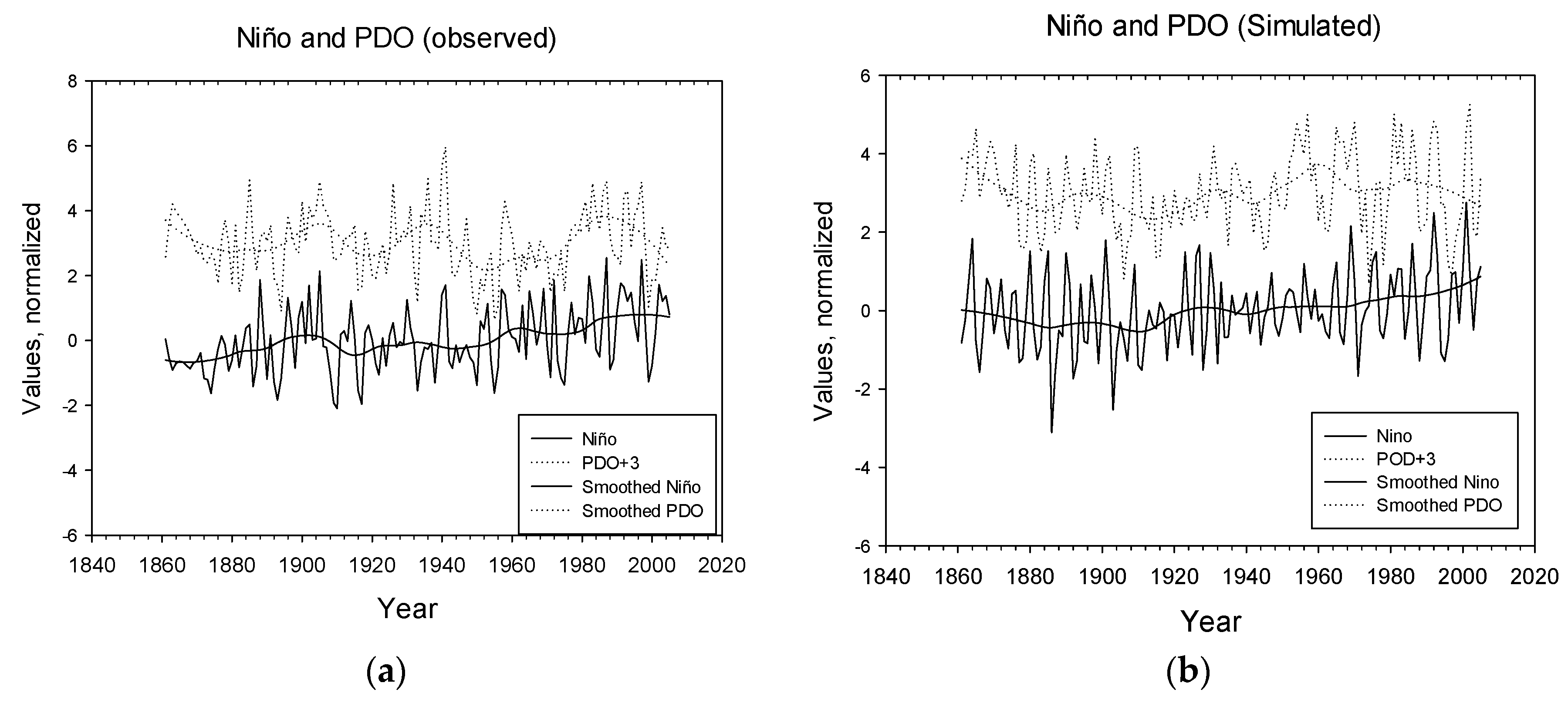
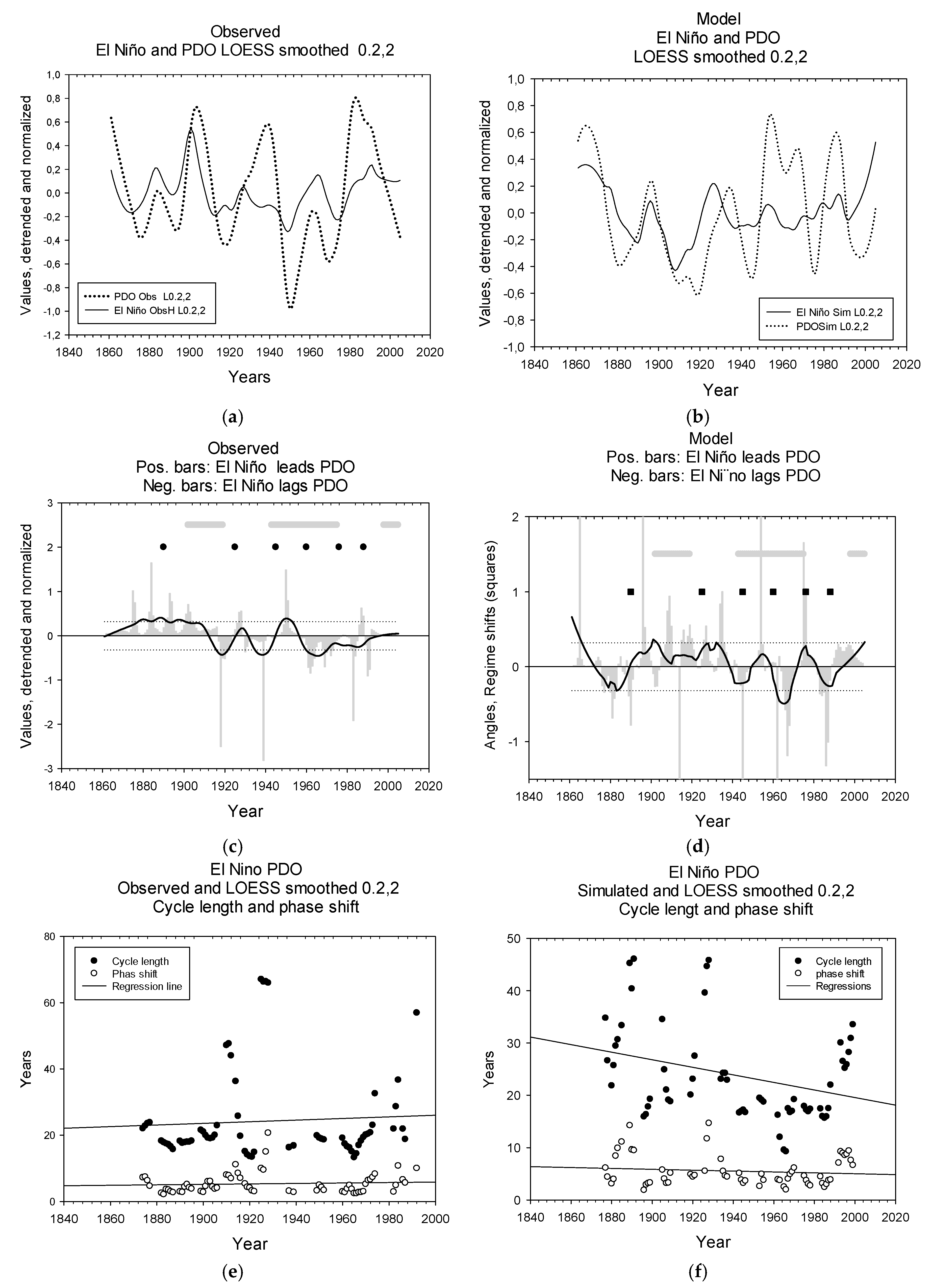
The observed El Niño and the observed PDO- index are shown in Figure 1a. The graphs show both the raw series and smoothed series (smoothing is discussed below). Corresponding simulated series are shown in Figure 1b.
The CO2 index measures CO2 emissions in pG/year. It is one of the drivers of the model. Compared to CO2 concentrations in the atmosphere, the multidecadal detrended pattern is shifted 2–3 years backward (not shown).
Annual, decadal and multidecadal variations. The high frequency variations are represented by the raw annual mean data and multidecadal cycles are represented by smoothed series.
Tie Pints, or Dated Events
Regime shifts. There appears to be a consensus that there are regime shifts or “changes in polarity” [4] in the global variables, although the exact meaning of what a regime shift constitutes is not clear [3]. Minobe [10] suggests regime shifts of alternating polarity in the Pacific sector around 1890, the 1920s, 1940s and 1976/1977. Chen and Wallace [11] suggest regime shifts in the 1920s, 1940s, 1970s and around 2000. Reid, Hari [4] show that a regime shift in the 1980s represented a major change in the Earth’s biophysical system. The shifts correspond to major shifts between positive and negative values for a new definition of a centered PDO proposed by Wills. It seems possible to summarize the shifts as occurring in 1890, 1920, 1945, 1960, 1976 and 1998.
Hiatus periods. The time series of GTA for global warming contains periods named “hiatus” periods when global warming ceases to increase. These periods are often determined to be 1902 to 1920, 1943 to 1975 and 1998 to 2014, although the exact timing is debatable, e.g., Trenberth and Fasullo [12], and more recently, Medhaug, Stolpe [13] and Hedemann, Mauritsen [14]. A third group of tie-points are the events associated with volcanic eruptions. However, the climatic effects of the eruptions may be associated with the formation and the recovery after the peak albedo that can occur 1 to 3 years after the actual eruption, [4,15].
3. Methods
In this section, we first describe pretreatment of our data. Thereafter, we give an outline of the methods used to apply the comparison tests between interactions in the observed and the modeled systems. One test, the quantifying of running LL-relationships, is not standard and is therefore addressed in more detail. In contrast to other methods, e.g., cross correlation, the LL-method calculates LL-relations based on 3 consecutive paired observations, and allows significance measures to be calculated for 9 consecutive pairs. This again allows for identification of dates in the series where a leading relation turns into a lagging relation or vice versa.
3.1. Pretreatment of the Data
Detrending and normalizing. We detrend the variables in this study by maintaining the residuals after a linear or a polynomial regression. A second order polynomial regression is applied to the CO2 series because this series shows a clear progressive increase with time. The series are then normalized to unit standard deviation. Since the paired data are measured in different units, normalizing just brings the data on a common scale, and the regression coefficient (the β-coefficient) becomes numerically equal to the r-statistics.
Smoothing. We use smoothing for two major purposes. Firstly, we smooth the raw time series to identify long term, multidecadal cyclic patterns, and secondly, we smooth the LL-results to emphasize patterns in results. To smooth the variables, we use the LOESS standard smoothing algorithm. The algorithm is available in many statistical packages, and here we use SigmaPlot© (San Jose, CA, USA). The smoothing algorithm has two variables. The first, (f), shows how large fraction of the series is used for calculating the running average. The second, (p), is the order of the polynomial function used to make interpolations. We always use p = 2. For calculation of leading-lagging, LL-relations, we use two versions of each variable: (i) the raw data and (ii) LOESS smoothed data with f = 0.1 to 0.3 and p = 2. To emphasize patterns in the figures showing rotational angles, we smooth the raw data, f = 0.2 and p = 2.
3.2. Quantifying Running Leading-Lagging Relation for Pairs of Variables
A leading relation is a prerequisite for a cause that imposes an effect on another variable. There are several methods available to establish LL-relations [16,17,18,19,20]. We adopt a method developed by Seip and McNown [21] that determines LL-relations for paired synoptic series of three observations, and allows calculation of confidence estimates for series of 9 consecutive observations. The method also addresses the problem of decomposing complex time series into meaningful “intrinsic mode” functions, e.g., Huang, Shen [20]. With the LL-method, we identify paired series where one precedes the other even if they do not contain clear peaks or troughs that would ease visualization of LL-relations.
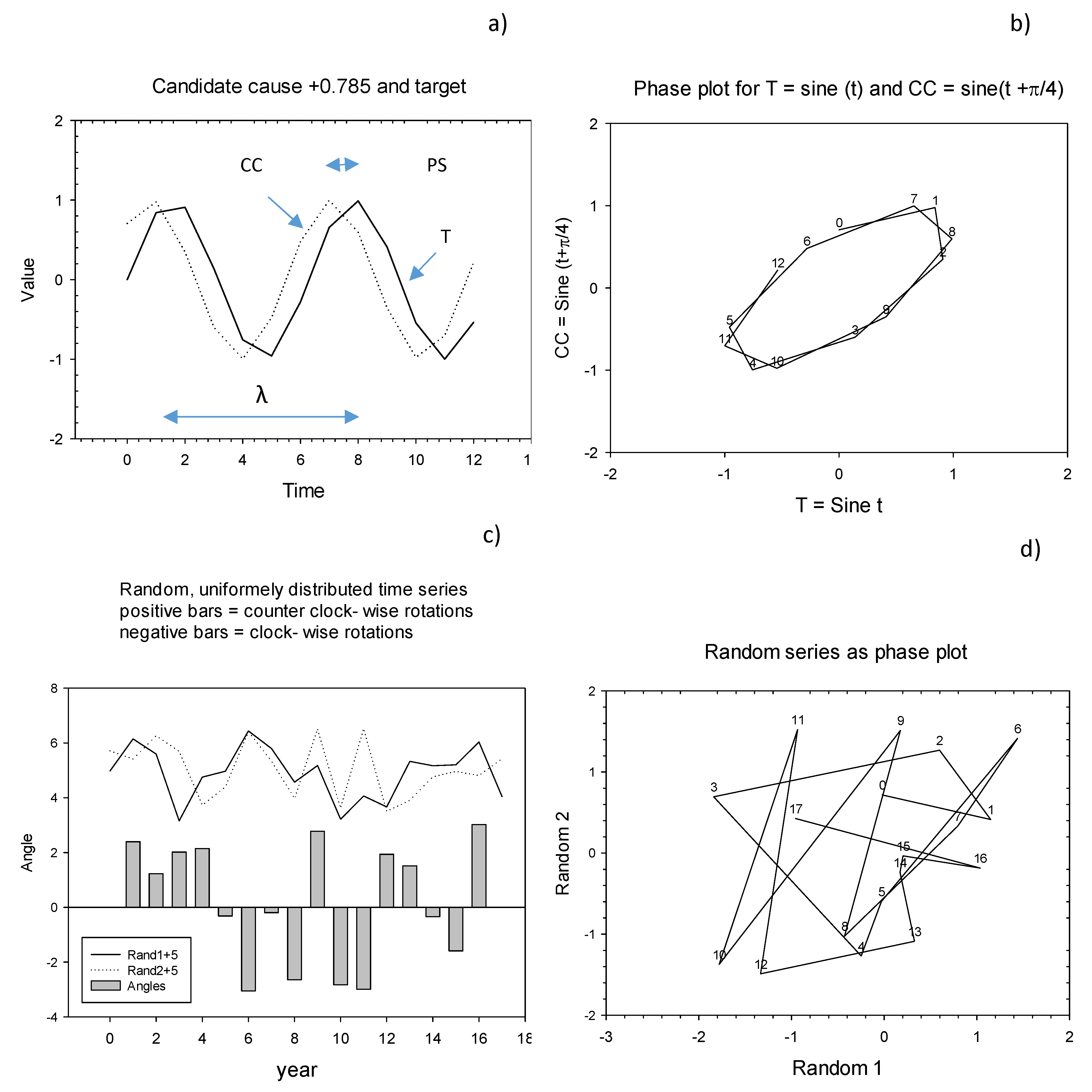
The LL-method consists of 5 steps and is explained with reference to Figure 2 and follows closely the description given in Seip and Grøn [22]. The duality between a time series representation and a phase plot representation below, has a counterpart in electrical engineering with the Lissajous curves that link the presentation of two time series x and y in time space, (t in the x-axis) to a presentation in phase space with the x-time series on the x-axis and the y-time series in the y-axis, e.g., https://en.wikipedia.org/wiki/Lissajous_curve. The equation 1 below has a counterpart in the calculation of magnetic fields around a wire, e.g., https://en.wikipedia.org/wiki/Biot%E2%80%93Savart_law.
As an example, we examine the LL-relations between two sine functions, the target, (T), and the candidate cause, (CC):
T = sin (t); CC = sin (t + ϕ), ϕ = π/4
The two functions are depicted in Figure 2a. We chose the example so that the candidate cause (CC), peaks before the target (T). With T depicted in the x-axis and CC in the y-axis, trajectories in the phase diagram rotate clockwise (Figure 2b).
LL-relations. To see which variable that comes (peaks) first, we quantify rotational directions by the formula in Equation (2). The angle, θ, is (It can be implemented in Excel format: With v1 = (A1, A2, A3) and v2 = (B1, B2, B3) in an Excel spread sheet, the angle is calculated by pasting the following Excel expression into C2: = SIGN((A2 − A1)*(B3 − B2) − (B2 − B1)*(A3 − A2))*ACOS(((A2 − A1)*(A3 − A2) + (B2 − B1)*(B3 − B2))/(SQRT((A2 − A1)2 + (B2 − B1)2)*SQRT((A3 − A2)2 + (B3 − B2)2)))).
where v1 and v2 are two successive vectors, through 3 consecutive points in the phase plot.
The LL-strength of the mechanisms that cause two variables to either rotate clockwise or counter clockwise in a phase portrait is measured by the number of positive rotations (counter clockwise rotations by convention) minus the number of negative rotations, relative to the total number of rotations over a certain period. In this study, it is 9 years.
LL = (Npos − Nneg)/(Npos + Nneg)
We use the nomenclature: LL(x, y) = [−1, 1] for LL-strength: LL (x, y) < 0 implies that y leads x, y→x; LL(x, y) > 0 implies that x leads y, x→y. The LL-strength for the series in Figure 2a is LL = −1. The positive (counter clockwise) and negative rotations for the paired random series in the upper part of Figure 2c are shown as positive and negative bars representing the angles θ in the lower part of the figure. A phase plot of the series is shown in Figure 2d. A significant LL-relation would show a more consistent pattern of negative or positive rotations as shown below on uncertainty estimates. Thus, LL-strength is itself a time series variable.
The cycle length, (CL), of two paired series that interact can be approximated by the partial ellipse method:
For sampled perfect sine functions, Equation (4) gives very closely the design length, 2π, of the sine functions. The cycle length we identified should ideally be based on full rotations in the phase plot for the paired time series, but noise or other superimposed signals may not allow full rotations to be completed as a significant series. In the example, we obtain CL = 6.30, which is close to the design cycle time of 2π = 6.28. In the present study, we plot cycle lengths as bars for n = 3.
The wedge in Figure 2b suggests how the formula works. It calculates the sum of angles, say over 9 wedges and the corresponding number of points that define them. (The angles with the top point in the origin correspond to the angles between successive trajectories.) The cycle length is the proportion of points required to fill a circle with wedges, that is an angle of 2π.
Phase shifts, (PS). The regression slopes, (s), or the β-coefficients, for cyclic series will give information on the shift, or time lag, between the series. If the two series co-vary exactly, their regression coefficient will be 1, and the time lag will be zero. If they are displaced half a cycle length, the series are counter-cyclic, and the regression coefficient is r = −1. Lead or lag times, PS, are estimated from the regression coefficient, (r), for sequences of 9 observations, PS (9). With λ as cycle length, an expression for the phase shift between two cyclic series can be approximated by:
PS ≈ λ/2π × (π/2 − Arcsine(r))
For r = 1, Arcsine = π/2, the right parenthesis is zero giving PS = 0. For r = −1, arcsine = −π/2 and the right parenthesis is 2 × π/2 = π and PS = λ /2.
The cycle length algorithm, Equation (4) will give an estimate that converges towards the ground truth (design value with sine functions) when averaged over increasing periods of the time series. whereas, the phase shift algorithm, Equation (5), requires that the sequence of points cover the whole cycle to give a good approximation.
Pro cyclisity and counter cyclisity. We define two sine—like functions to show a pro-cyclic relation if the phase angle (ϕ) is less than λ/2 in absolute value. With ϕ outside this range, a phase plot for the two functions will show a negative, s, and the two functions are counter- cyclic.
Uncertainty estimates. To find an expression for the uncertainty in our LL-strength estimates we ran Monte Carlo simulations on two paired uniformly random series. In the present study, we calculated running averages of the LL-strength over periods of 9 years. We treated the periods conservatively by assigning them significant LL-strength only if LL < −0.32 or LL > +0.32. In addition, at least three successive observations were required to be within a significant period. The criterion chosen is a tradeoff between confidence in the results and the possibility of detecting changing LL-relations. We made all calculations in Excel and with figures drawn in SigmaPlot 11© (San Jose, CA, USA). We also examined if a pair of random time series would show apparent cycles. We found that cycles longer than 5 time steps (here representing 5 years) would occur less than one in 20 times, corresponding to p < 0.05.
3.3. Auxiliary Methods
The power spectral density (PSD) is measured with the standard algorithm found in SigmaPlot© (San Jose, CA, USA). We applied PSD to the LL-series for the 3 observed pairs of the time series between El Niño, PDO, and CO2 and the 3 observed pairs of the corresponding smoothed series. We then stacked the 6 series to see if there would be dominating cycles in the observed system assuming that non-dominating peaks in the PSD cancel out. The same procedure was made for the simulated series. Ordinary linear regressions (OLR) were calculated with the standard algorithm found in SigmaPlot© (San Jose, CA, USA). However, any standard methods could be used. Lastly, we calculated the running average slope (n = 10) for GTA, LOESS smoothed the series, f = 0.2, p = 2 and identified the hiatus periods as those with negative slopes or slopes less than 1/20 of the range in slopes.
4. Results
We first examine the relations between pairs of variables derived from observed data and from simulated data. We thereafter show the results for LL-relations between the pairs and lastly we examine the common cycle times and phase shifts between the pairs
A. Regressions between pairs of observed series and pairs of simulated series. The observed and the simulated raw series for the El Niño and PDO are shown in Figure 1a,b. The multidecadal series obtained by smoothing the raw series (LOESS smoothed with f = 0.2 and p = 2) were shown as series superimposed on the raw series. The observed raw series and the observed multidecadal (low frequency) series for the El Niño and PDO correlate p < 0.05 (Table 1). The same occurred for the simulated raw and simulated multidecadal series for the El Niño and PDO, p < 0.001. However, the observed and the simulated raw and multidecadal (low frequency) series for El Niño and PDO did not correlate, p > 0.08.
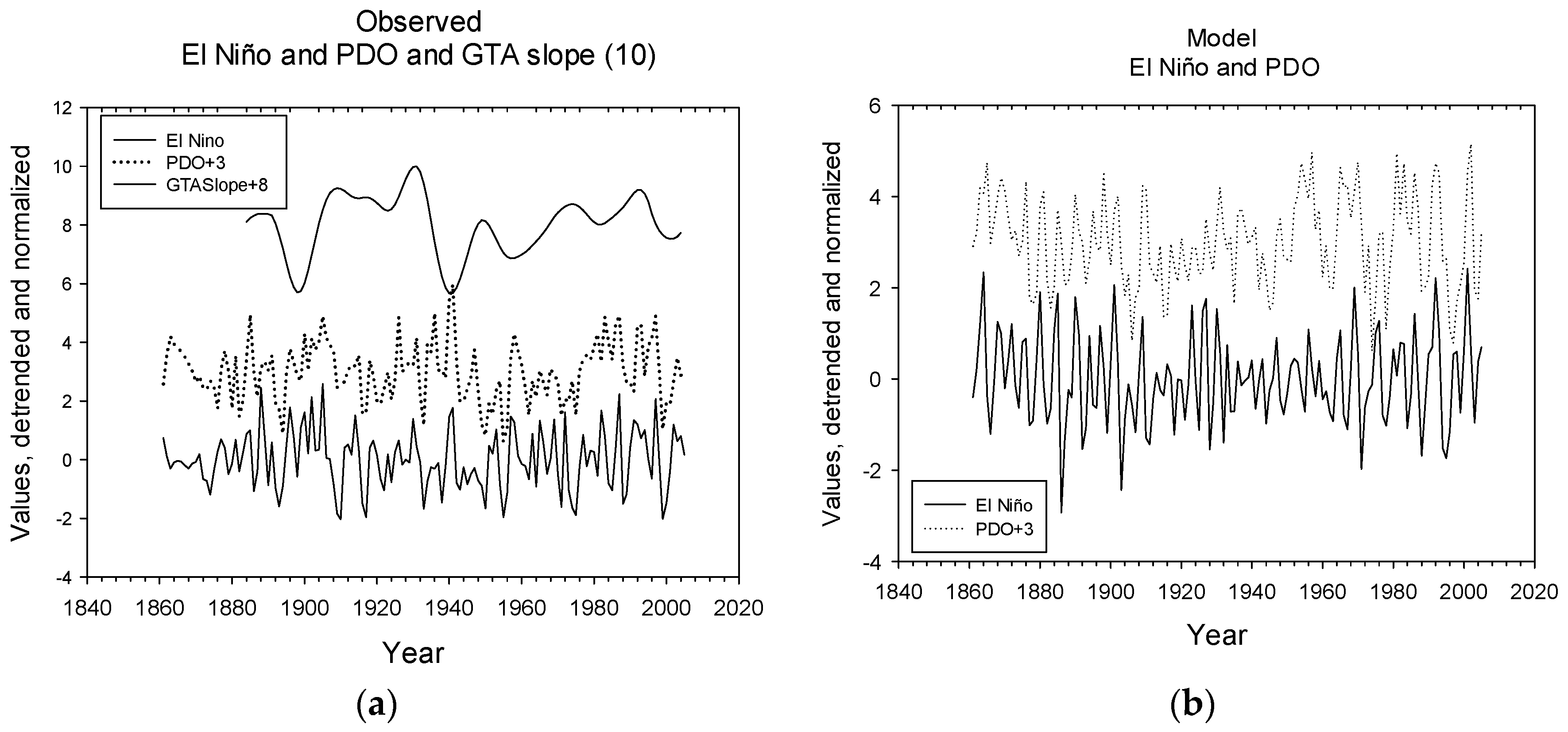
B. The leading-lagging relations between the El Niño and PDO. Figure 3a shows the observed raw, but detrended and normalized, time series for the El Niño and PDO and Figure 3b the corresponding modelled time series. The LL-relations between the El Niño and PDO are shown in Figure 3c (observed) and 3d (simulated). Grey bars represent LL-relations so that a positive bar shows that the El Niño leads PDO and a negative bar shows that the El Niño lags PDO. A smoothed line characterizes the main pattern for LL-relations. The dashed lines denote confidence limits. The figure shows that El Niño is an overall leading variable to PDO, but there are periods where the LL-strength is weak, or opposite. Figure 3d shows the corresponding LL-relations found for the simulated pair of El Niño and PDO. The El Niño is a more persistent leading variable to PDO in the simulated series than in the observed series. For both the observed and the simulated pairs, the El Niño appears to be a less strong leader to PDO around 1910, 1960 and 2000. These years correspond approximately to hiatus periods (grey horizontal bars) but only to some years designated as regime shifts (black squares). However, a regression between the observed and simulated LL-strength series is non-significant, p > 0.1.
The LL-strength is pro-cyclic with El Niño from 1861 to about 1960, Slope (LL-strength, El Niño) >0, as shown by the running average slope time series in Figure 3c. It is undetermined after 1960, but its changing pattern still may resemble that of the simulated pattern, c.f., the peak in 1937–1938 for both series. There is no significant relation between the LL-strength and either El Niño or PDO in the simulations.
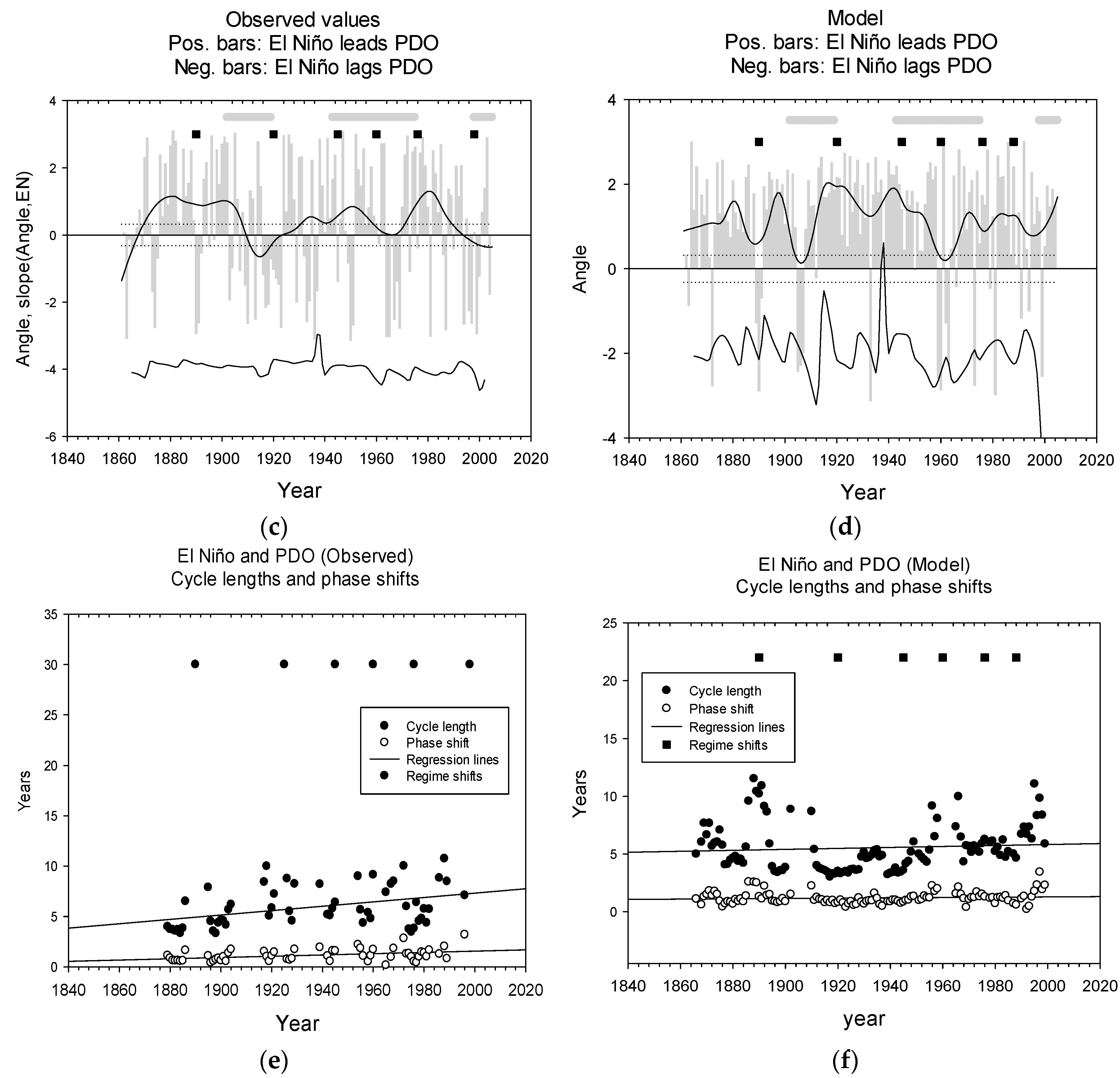
The El Niño and the PDO series were both LOESS smoothed (same parameter sets in the LOESS algorithm) to identify multidecadal cycles (Figure 4a,b). The smoothing was a little less strong than the 12-year Lanczos low pass-filtered PC1 for the PDO reported in Chen and Wallace [11]. Both the observed and the simulated LL-relations still showed that the El Niño tended to lag the PDO during 1910–1920 and the 1960s, but in addition, there seems to be a period around 1940 when the El Niño lagged the PDO (Figure 4c,d). The year 1940 is among the regime shift years and close to the beginning of the hiatus period 1943–1975. The smoothing algorithm may distort the endpoints of the series so we do not treat information from before 1880 or after 2000 as significant.
Since we only have 3 hiatus periods, we also compared the interaction patterns in Figure 3c,d with a time series for a running average slope (n = 10) of the GTA. We examined the mid period 1921 to 1993 to avoid end values (smoothing distorts end values). The hiatus period 1943 to 1975 is thus included. The results for raw, high frequency and smoothed, low frequency data are shown in Table 1. For the observed data, only the low frequency regression is statistically significant p < 0.01; whereas for the simulated data both high and low frequency pattern are significant, p < 0.001. During the period 1921 to 1993 there were periods where increasing impact of El Niño on PDO were both leading and lagging changes in GTA.
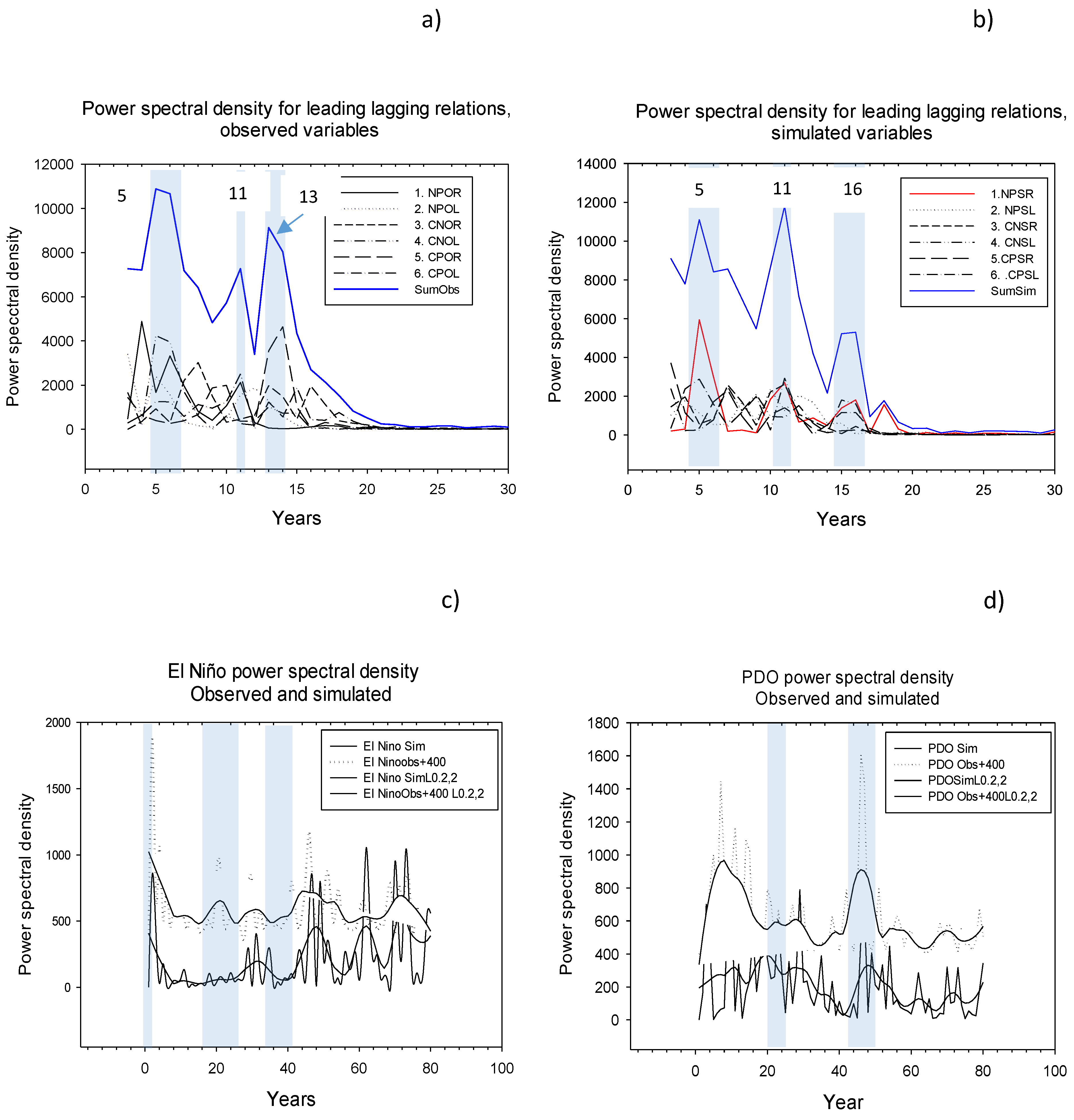
C. Power spectral density of LL-relations. The LL-series shifted several times between being leading and lagging during the period from 1861 to 2005, we also applied PSD analysis to the LL-relations (Figure 5a,b). Since we wanted to characterize the teleconnections system, we stacked all PSD plots to see if some cycle lengths would reinforce each other, while others would annihilate each other. The peaks in the PSD for the stacked observed LL-relations are shown in Table 2, row I. The PSD showed major peaks at 5, 11 and 13 years. The PSD for the stacked, simulated LL-relations showed major peaks at 5, 11 and 16 years. Both PSDs also showed minor peaks around 26 and 31 years (not shown in the PSD graphs).
D. Power spectral densities for single series. We show the power spectral series both as raw data and smoothed, to emphasize major features. For the single series we included cycle lengths up to 80 years because Minobe [10] suggests that there might be 50 to 70 year cycles over the North Pacific, Figure 5c and d. However, our time series are too short so that results for longer cycles would only be suggestive. We therefore report cycle length results for the short range (0–32 years) and the long range (33–70 years) separately. There are peaks at similar cycle length in both the observed and the simulated data. In the short cycle length range, we found a cycle length of 21 and 31 years for the observed El Niño and 11 and 32 years for the simulated El Niño. For the observed PDO we found cycle lengths of 8, 22 and 28 years and for the simulated PDO at 7, 11, 20 and 31 years. In the long cycle range, 33 years and above, we found similar cycles for the two time series around 44–49, 62 and 70–72 years , Table 2, Row II and III.
E. Cycle lengths for paired time series. With the partial ellipse method, we estimated the common cycle length by averaging cycle lengths. For the observed variables, we found 7.9 ± 2.5 years for the raw series and 24.5 ± 3.2 years for the smoothed series, Figure 3e and Figure 4e. Corresponding estimates for the simulated variables were 8.4 ± 4 years and 23.9 ± 3.0 years, Figure 3f and Figure 4f. The cycle length for the observed and the smoothed series was in no cases statistically different.
F. Phase shift. The values for phase shifts were 1.18 ± 0.5 years, 1.19 ± 0.53 years for the raw observed and simulated data, 4.6 ± 4.7 years, and 4.9 ± 4.6 years for the smoothed observed and simulated data.
5. Discussion
An annotated summary of the results is given in Table 3. Since simulations depend upon exogenous variables (e.g., CO2 emissions), we also suggest years when observations or simulations, or both, indicate particular events.
5.1. Raw and Smoothed Time Series
Inspecting the series for the El Niño and PDO visually, both sets show similar patterns, for example, with a peak starting in 1980 and ending in 2000. Although observed series for the El Niño—like variability are retrieved from different but some overlapping regions in the Pacific, they are reported to show similar characteristics when smoothed [11]. Also, the various PDO series appear to show similarities and express properties of the Pacific ocean over large regions [24].
Thus, our choice of the smoothing algorithm and smoothing parameters is supported. In simulations, the effects of the initial conditions will disappear after approximately one year.
There is no canonical way to find an optimal smoothing for a time series with noise or for complex time series that are a superposition of several time series with different cycle lengths or different phase shifts. In the El Niño, PDO pair studied here, the PDO is likely a superposition of several different physical mechanisms [25]. In the literature, several approaches have been used to disentangle component cycles [11,19,26,27,28].
5.2. Paired Series
We first discuss our smoothing process and thereafter the results for the paired series. It appears that interactions, as measured by the LL-relations for observed and simulated series have some important common characteristics that should be useful for further analyzing model simulations.
A. Regressions. A linear regression between the El Niño and PDO shows a significant correlation both in the observed set and in the simulated one. Since the model is partly driven by observed forcing, like CO2 emissions, trends and deviations from the trends in the driving forces may be reproduced in the simulated values. However, the simulated and the observed series for both El Niño and PDO did not correlate p > 0.1. Thus, even though both El Niño and PDO visually show common characteristics, the OLS did not capture their similarity as significant. However, shifting one series relative to the other may improve correlation. The LL-technique discussed below addresses this cross-correlation issue.
B. LL-relations. When we say that one series leads another, the interpretation is that peaks (or troughs) in the leading series are in front of peaks (or troughs) in the target series and closer than ½ of their common cycle length, (λ). However, very long leading times may occur that exceed ½ λ. Secondly, two series that show LL-signatures may be driven by a third series, but with phase shifts relative to this series. Using the leading series for prediction is still possible, but the leading series need not have a causal effect on the second series. The latter is common in biological systems where one species reacts slower to, for example, warming than another [29].
The LL-relations for the El Niño and PDO showed a general tendency for the El Niño to lead the PDO, but during the 1910s and during the 1960s and 2000 (Figure 3c,d and Figure 4c,d) El Niño lag PDO. The 1910s, the 1960s and the 2000s are presented as hiatus periods (1902–1920, 1943–1975, 1998–2014) and also as regime shifts or “tie” dates by several authors (listed in the material section).
There are at least 3 other dates that are presented as regime shifts (1890, 1945, 1976 and the 1980s), but they are not distinctly present in the LL-relations, nor in the simulated PDO. In line with Imbrie, Berger [30]’s comment on “the curious incident of the dog that did not bark” [31], the absence of a response to a stimulus is also an important clue that some information may be missing in the model.
The hiatus periods seem to be related to periods when the El Niño has a weak impact on PDO. It is interesting that from 1861 to about 1960, the observed function: LL(El Niño, PDO) = s × El Niño shows a positive slope, s > 0, that is the two time series are pro-cyclic, but after 1960 pro-cyclisity ceases. The corresponding function for the simulated variables shows no consistent slope, but still there are events where the observed and the simulated slope patterns show similarities, e.g., a peak in 1937–1938.
The next three sections discuss cycle lengths. The first concerns cycle lengths for the time series that show the LL-relations. The second examines cycle lengths for single series and the third examines common cycle lengths for paired series.
C. The power spectral density for LL-relations (El Niño, PDO and CO2 series), shows that the cycle length is similar for the observed and the simulated series. Both show major peaks at 5 and 11 years, (Figure 5a,b). In the simulated variables, there is also a pronounced 16 years cycle. Both series also show peaks at 26 and 31 years (not shown in graphs). The peaks suggest that there are cycles in the LL-strength, but the results in Figure 3c,d show that the PDO is a leading variable to El Niño only two or three times during our 140-year study period. Since these events occur very closely at the same time both in the observations and in the simulations, it should be possible to identify almost exactly why these events occur.
D. Power spectral density for the single series. Since spectra for six paired series (El Niño, PDO, CO2, raw versions and LOESS smoothed) show common characteristics, we compared superimposed spectra from the observed series to superimposed spectra based on the random series (not shown). We conclude that the spectra based on observed and simulated time series represent real signals because peaks stand out more clearly in the PSD graphs based on the observed series than on those based on the random series. We have not developed a significance test for this case. Our results on the short cycle lengths showed that the El Niño did not have a marked peak below 11 years, but there were several smaller peaks. Our results on the long cycle lengths > 32 years suggest that distinct long cycles exist, but the time series used are too short to establish such cycles with certainty.
E. Common cycle lengths. The cycle length found with the partial ellipse method was 7.9 ± 2.5 years based on the raw series and 24.5 ± 3.2 years based on the smoothed series.
We estimated cycle lengths for the El Niño and PDO with the PSD algorithm and compared the results to the estimates for the common cycles found with the partial ellipse method. Our assumption is that the partial ellipse method will extract common cycle lengths from the two time series in a pair and disregard other cycle lengths that are not common. For the short cycle lengths based on the raw series, we found that the PDO showed cycle lengths of comparable size, 7–8 years, but the El Niño showed no distinct cycle lengths below 11 years. Still, the fuzzy peak pattern below 11 years in the PSD graphs may represent cycles that are sufficient to define a common cycle around 8 years. For the long cycles, based on the smoothed data, 24–25 years, and the partial ellipse method extract cycles in the range 20–31 years from both El Niño and PDO, Table 2. This result can be compared to the tests for “intrinsic mode functions” used to decompose complex time series ([20] p. 915) that also show major contributing cycle lengths in composite cyclic series.
Cycles in LL-relations and cycles in contributing series. There is a possibility that cycles in the LL(El Niño, PDO) series reflect cycles in either El Niño or PDO. We found that the LL-time series might reflect the El Niño time series in the observations from 1861 to 1960, but not later. There was no such breakpoint in the simulated series. The years around 1960 have been designated as a breakpoint in the oscillation volatility by Torrence and Webster [32] and Kestin, Karoly [19].
The reality of cycle lengths. Even though we find distinct cycle lengths, there are arguments that the cycle lengths are the results of artefacts in the methods. For example, [33] shows that peaks in power spectra may be due to red noise and that sharp spectral lines in climate records may be due to aliasing effects. Seip and Grøn (2017) show that if one random series interacts with another series to impose a similar random pattern on the latter series, the two series may show distinct cycles. Furthermore, two random series that are plotted in a phase plot (random 1 in the x-axis and random 2 in the y-axis) will show frequent rotations of their trajectories in the same direction for 3 to 5 time steps. but then ”same rotation direction” will rapidly be reduced (more than 5 in a sequence has a probability of less than 1 in 20 to occur.) Thus, cycle lengths of 7 years and longer suggest that the paired series co-vary and that the processes that generate them are real. Since cycle lengths ≥7 years are frequent, our results support the hypotheses that ocean basins interact, but few climate model studies include such couplings [34].
F. Phase shift. Phase shifts are normally found by cross correlation, and the results with the LL-method can be compared to results by this method. Covariances between El Niño, PDO and CO2 are observed by Patra, Maksyutov [35]. The shift between the time series are about ¼ of a cycle length both for the short cycle length of the high frequency series and the long cycle length of the low frequency series suggesting that the El Niño and PDO will appear as orthogonal in PCA plots as shown by Wills, Schneider [9].
5.3. Comparing Observations and Simulations
There are several similarities in the observations and simulations. For example, the LL-strength between the El Niño and PDO shows strong similarities to the El Niño time series until 1960. The hiatus periods appear to occur when El Niño ceases to be a leading variable to PDO. It is also interesting that the slope between the El Niño series and the LL(El Niño, PDO) shows a peak in 1937–1938 suggesting that there are mechanisms in the system that increase El Niño and at the same time increase the leading strength of the El Niño relative to the PDO. There are also similarities in cycle lengths and in phase shifts.
Cyclic time series seldom satisfy standard assumptions for applying regression analysis. For example, normality and power tests normally fail even though the analysis may calculate explained variances and probability. Furthermore, interpretation of results is different from for normally distributed number series. However, in spite of such shortcomings, we selected the period 1921 to 1993, n = 73, and applied linear regression analysis to (i) the series that express the impact of El Niño and PDO on each other, (Ang (EN, P) in Figure 3c,d) and (ii) the GTA slope. The rationale for selecting only the midpoint of the series is that the series become distorted at their ends when they are smoothed or averaged. However, the period includes the 1943 to 1975 hiatus. Since the potential effect of one of the variables may be delayed with respect to the other, we applied cross correlation by shifting the series with time so that the regression would give optimum explained variance. The simulated series gave significant correlations, p < 0.001 and relatively high explained variance ≈44%. The observed series gave significant results for the smoothed, low frequency series, but low explained variance ≈10%, Table 1. We did not try to correct for regression assumptions that were not passed. Although regression analysis applied to cyclic series have drawbacks, we believe that the visual results for observations and simulation (Figure 3 and Figure 4) and our regression results support the hypothesis that the hiatus periods are closely associated with a weakening of the impact of El Niño on PDO.
There are driving variables in the model that may act as tie-points to create simultaneous events. CO2 emissions were used as an exogenous driving force in the model and changes in the atmosphere CO2 concentrations may change global warming system, including ocean circulations. Several authors also assign a role to volcanic eruptions and the subsequent albedo effects. For example, Mehta et al. [36] lists four major, low latitude volcanic eruptions that are associated with phase transitions in the PDO. Reid, Hari [4] attribute the global impacts in 1980 partly to the recovery from the El Chichón volcanic eruption in 1982 and Stevenson, Otto-Bliesner [15] suggest that both Northern and Tropical eruptions favor El Niño initiations. If there are triggering events, like volcanic eruptions, that ultimately cause hiatus periods, then their occurrence cannot be predicted. However, it should not be possible to associate the hiatus periods with other events than volcanic eruptions, but ocean interactions also appear to play a role.
Second, other events may be attributed to changes in carbon sequestering by the oceans [37], changes in SST [38], or changes in the Earth’s energy budget [39]. Third, still other events or regularities may be the result of inherent properties of stochastic ocean movements that interact [40]. In the present study, we only address leading lagging relations that are a prerequisite for a causal effect, but not sufficient. To establish causation with greater strength, physical mechanisms would give credibility to the potential causal relation. It is beyond the present study to give a summary of such mechanisms. Furthermore, there are more candidate variables that have been suggested in the literature as causal agents for global warming, and a selection of these variables is the objective of a new study.
6. Conclusions
Interactions described by leading–lagging LL-relations for the observed and simulated values were surprisingly similar. Both showed that the El Niño is leading the Pacific decadal oscillation most of the time in the period 1861–2005, but both also show that there are exceptions around 1910, 1960 and 2000 where the lead is weak, or where El Niño lags PDO. These periods correspond approximately to the hiatus periods. With LL-relation between paired series, an implicit assumption is that the two series show the same cyclic behavior. We found that in the short-cycle length range (0–35 years) the cycle lengths around 7 and 20 years were present in both observations and simulations. In the long cycle length range cycle lengths around 30, 26 and 72 years were present in both observations and simulations. However, there are also differences between the observed and simulated results that could give input to closer examinations between external forcings and possible factors that could trigger regime shifts and should be included in global climate models.
Our study is based on detrended series. Thus, variations in the time series that could be associated with smoothly increasing greenhouse gases are not included.
Author Contributions
For research articles with several authors, a short paragraph specifying their individual contributions must be provided. The following statements should be used “Conceptualization, K.L.S. and H.W.; Methodology, K.L.S.; Software, K.L.S.; Validation, K.L.S., H.W. and H.W.; Formal Analysis, K.L.S. Investigation, K.L.S. and H.W.; Resources, K.L.S.; Data Curation, K.L.S. and H.W.; Writing-Original Draft Preparation, K.L.S. and H.W.; Writing-Review & Editing, H.W. and K.L.S.; Visualization, K.L.S.; Supervision, K.L.S .and H.W.; Project Administration, H.W. and K.L.S.
Funding
This research received no external funding.
Acknowledgments
We would like to thank OsloMet-Oslo Metropolitan University for funding Knut L. Seip. There are no conflicts of interest. We would also like to thank David Wang for reading the manuscript and suggesting improvements, and four anonymous reviewers for their insightful and constructive comments and suggestions.
Conflicts of Interest
The authors declare no conflict of interest.The funders had no role in the design of the study; in the collection, analyses, or interpretation of data; in the writing of the manuscript, and in the decision to publish the results.
References
- Wang, S.Y.; L’Heureux, M.; Yoon, J.H. Are Greenhouse Gases Changing ENSO Precursors in the Western North Pacific? J. Clim. 2013, 26, 6309–6322. [Google Scholar] [CrossRef]
- Taylor, E.K.; Stouffer, R.J.; Meehl, G.A. An Overview of Cmip5 and the Experiment Design. Bull. Am. Meteorol. Soc. 2012, 93, 485–498. [Google Scholar] [CrossRef]
- Overland, J.; Rodionov, S.; Minobe, S.; Bond, N. North Pacific regime shifts: Definitions, Issues and Recent Transitions. Prog. Oceanogr. 2008, 77, 92–102. [Google Scholar] [CrossRef]
- Reid, P.C.; Hari, R.E.; Beaugrand, G.; Livingstone, D.M.; Marty, C.; Straile, D.; Barichivich, J.; Goberville, E.; Adrian, R.; Aono, Y.; et al. Global Impacts of the 1980s Regime Shift. Glob. Chang. Biol. 2016, 22, 682–703. [Google Scholar] [CrossRef] [PubMed] [Green Version]
- Parrenin, F.; Masson-Delmotte, V.; Kohler, P.; Raynaud, D.; Paillard, D.; Schwander, J.; Barbante, C.; Landais, A.; Wegner, A.; Jouzel, J. Synchronous Change of Atmospheric CO2 and Antarctic Temperature during the Last Deglacial Warming. Science 2013, 339, 1060–1063. [Google Scholar] [CrossRef] [PubMed] [Green Version]
- Mehta, V.M.; Wang, H.; Mendoza, K. Decadal Predictability of Tropical Basin Average and Global Average Sea Surface Temperatures in CMIP5 Experiments with the HadCM3, GFDL-CM2.1, NCAR-CCSM4, and MIROC5 Global Earth System Models. Geophys. Res. Lett. 2013, 40, 2807–2812. [Google Scholar] [CrossRef]
- Trenberth, K.E. Has There Been a Hiatus? Science 2015, 349, 691–692. [Google Scholar] [CrossRef] [PubMed]
- Gehne, M.; Kleeman, R.; Trenberth, K.E. Irregularity and Decadal Variation in ENSO: A Simplified Model Based on Principal Oscillatory Petterns. Clim. Dyn. 2014, 43, 3327–3350. [Google Scholar] [CrossRef]
- Wills, R.C.; Schneider, T.J.; Wallace, M.; Battisti, D.S.; Hartmann, D.L. Disentangling Global Warming, Multidecadal Variability, and El Nino in Pacific Temperatures. Geophys. Res. Lett. 2018, 45, 2487–2496. [Google Scholar] [CrossRef]
- Minobe, S.A. 50–70 Year Climatic Oscillation over the North Pacific and North America. Geophys. Res. Lett. 1997, 24, 683–686. [Google Scholar] [CrossRef]
- Chen, X.Y.; Wallace, J.M. ENSO-Like Variability: 1900–2013. J. Clim. 2015, 8, 9623–9641. [Google Scholar] [CrossRef]
- Trenberth, K.E.; Fasullo, J.T. An apparent Hiatus in Global Warming? Earths Future 2015, 1, 19–32. [Google Scholar] [CrossRef]
- Medhaug, I.; Stolpe, M.B.; Fischer, E.M.; Knutti, R. Reconciling Controversies about Global Warming Hiatus. Nature 2017, 545, 41–47. [Google Scholar] [CrossRef] [PubMed]
- Hedemann, C.; Mauritsen, T.; Jungclaus, J.; Marotzke, J. The Subtle Origins of Surface-Warming Hiatuses. Nat. Clim. Chang. 2017, 7, 336. [Google Scholar] [CrossRef]
- Stevenson, S.; Otto-Bliesner, B.; Fasullo, J.; Brady, E. El Nino Like Hydroclimate Responses to Last Millennium Volcanic Eruptions. J. Clim. 2016, 29, 2907–2921. [Google Scholar] [CrossRef]
- Granger, C.W.J. Investigating Causal Relations by Econometric Models and Cross-Spectral Methods. Econometrica 1969, 37, 424–438. [Google Scholar] [CrossRef]
- Sugihara, G.; May, R.; Ye, H.; Hsieh, C.H.; Deyle, E.; Fogarty, M.; Munch, S. Detecting Causality in Complex Ecosystems. Science 2012, 338, 496–500. [Google Scholar] [CrossRef] [PubMed]
- Stips, A.; Macias, D.; Coughlan, C.; Garcia-Gorriz, E.; Liang, X.S. On the Causal Structure between CO2 and Global Temperature. Sci. Rep. 2016, 6, 21691. [Google Scholar] [CrossRef] [PubMed]
- Kestin, T.S.; Karoly, D.J.; Yang, J.I.; Rayner, N.A. Time-Frequency Variability of ENSO and Stochastic Simulations. J. Clim. 1998, 11, 2258–2272. [Google Scholar] [CrossRef]
- Huang, N.E.; Shen, Z.; Long, S.R.; Wu, M.C.; Shih, H.H.; Zheng, Q.N.; Yen, N.C.; Tung, C.C.; Liu, H.H. The Empirical Mode Decomposition and the Hilbert Spectrum for Nonlinear and Non-Stationary Time Series Analysis. Proc. R. Soc. Math. Phys. Eng. Sci. 1998, 454, 903–995. [Google Scholar] [CrossRef]
- Seip, K.L.; McNown, R. The Timing and Accuracy of Leading and Lagging Business Cycle Indicators: A new Approach. Int. J. Forecast. 2007, 22, 277–287. [Google Scholar] [CrossRef]
- Seip, K.L. and Grøn, O. Leading the Game, Losing the Competition: Identifying Leaders and Followers in a Repeated Game. PLoS ONE 2016, 11, e0150398. [Google Scholar] [CrossRef] [PubMed]
- Seip, K.L.; Grøn, Ø. A New Method for Identifying Possible Causal Relationships between CO2, Total Solar Irradiance and Global Temperature Change. Theor. Appl. Climatol. 2017, 127, 923–938. [Google Scholar] [CrossRef]
- Newman, M.; Shin, S.I.; Alexander, M.A. Natural Variation in ENSO Flavors. Geophys. Res. Lett. 2011, 38, 65. [Google Scholar] [CrossRef]
- Newman, M.; Alexander, M.A.; Ault, T.R.; Cobb, K.M.; Deser, C.; Lorenzo, E.D.; Mantua, N.J.; Miller, A.J.; Minobe, S.; Nakamura, H.; et al. The Pacific Decadal Oscillation, Revisited. J. Clim. 2016, 29, 4399–4427. [Google Scholar] [CrossRef]
- Huang, N.E.; Wu, M.C.; Long, S.R.; Shen, S.S.P.; Qu, W.D.; Gloersen, P.; Fan, K.L. A Confidence Limit for the Empirical Mode Decomposition and Hilbert Spectral Analysis. Proc. R. Soc. Math. Phys. Eng. Sci. 2003, 459, 2317–2345. [Google Scholar] [CrossRef]
- Wu, S.; Liu, Z.Y.; Zhang, R.; Delworth, T.L. On the Observed Relationship between the Pacific Decadal Oscillation and the Atlantic Multi-Decadal Oscillation. J. Oceanogr. 2011, 67, 27–35. [Google Scholar] [CrossRef]
- Power, S.; Haylock, M.; Colman, R.; Wang, X. The predictability of interdecadal changes in ENSO activity and ENSO teleconnections. J. Clim. 2006, 19, 4755–4771. [Google Scholar] [CrossRef]
- Seip, K.L.; Reynolds, C.S. Phytoplankton Functional Attributes along Trophic Gradient and Season. Limnol. Oceanogr. 1995, 40, 589–597. [Google Scholar] [CrossRef]
- Imbrie, J.; Berger, A.; Boyle, E.A.; Clemens, S.C.; Duffy, A.; Howard, W.R.; Kukla, G.; Kutzbach, J.; Martinson, D.G.A.; Mcintyre, A.C.; et al. On the Structure and Origin of Major Glaciation Cycles 2. The 100,000-Year Cycle. Paleoceanography 1993, 8, 699–735. [Google Scholar] [CrossRef]
- Doyle, A.C. The memoirs of Sherlock Holmes; George Newnes: Lonton, UK, 1893. [Google Scholar]
- Torrence, C.; Webster, P.J. Interdecadal Changes in the ENSO-Monsoon System. J. Clim. 1999, 12, 2679–2690. [Google Scholar] [CrossRef]
- Wunsch, C. The Interpretation of Short Climate Records, with Comments on the North Atlantic and Southern Oscillations. Bull. Am. Meteorol. Soc. 1999, 80, 245–255. [Google Scholar] [CrossRef] [Green Version]
- Knutson, T.R.; Sirutis, J.J.; Zhao, M.; Tuleya, R.E.; Bender, M.; Vecchi, G.A.; Villarini, G.; Chavas, D. Global Projections of Intense Tropical Cyclone Activity for the Late Twenty-First Century from Dynamical Downscaling of CMIP5/RCP4.5 Scenarios. J. Clim. 2015, 28, 7203–7224. [Google Scholar] [CrossRef]
- Patra, P.K.; Maksyutov, S.; Ishizawa, M.; Nakazawa, T.; Takahashi, T.; Ukita, J. Interannual and Decadal Changes in the Sea-Air CO2 Flux from Atmospheric CO2 Inverse Modeling. Glob. Biogeochem. Cycles 2005. [Google Scholar] [CrossRef]
- Mehta, V.M.; Mendoza, K.; Wang, H. Predictability of Phases and Magnitudes of Natural Decadal Climate Variability Phenomena in CMIP5 Experiments with the UKMO HadCM3, GFDL-CM2.1, NCAR-CCSM4, and MIROC5 Global Earth System Models. Clim. Dyn. 2017. [Google Scholar] [CrossRef]
- DeVries, T.; Holzer, M.; Primeau, F. Recent increase in carbon uptake driven by weaker upper-ocean overturning. Nature 2017, 542, 215–220. [Google Scholar] [CrossRef] [PubMed]
- Meehl, G.A.; Hu, A.; Arblaster, J.M.; Fasullo, J.; Trenberth, K.E. Externally Forced and Internally Generated Decadal Climate Variability Associated with the Interdecadal Pacific Oscillation. J. Clim. 2013, 26, 7298–7310. [Google Scholar] [CrossRef] [Green Version]
- Loeb, N.G.; Thorsen, T.J.; Norris, J.R.; Wang, H.; Su, W. Changes in Earth’s Energy Budget during and after the “Pause” in Global Warming: An Observational Perspective. Climate 2018, 6, 18. [Google Scholar] [CrossRef]
- Seip, K.L.; Grøn, Ø. On the Statistical Nature of Distinct Cycles in Global Warming Variables. Clim. Dyn. 2016. [Google Scholar] [CrossRef]
Figure 1.
Observed and simulated values for the El Niño and the Pacific decadal oscillation (PDO). (a) Observed value and smoothed values. (b) Simulated values; raw and smoothed values.
Figure 1.
Observed and simulated values for the El Niño and the Pacific decadal oscillation (PDO). (a) Observed value and smoothed values. (b) Simulated values; raw and smoothed values.

Figure 2.
Relation between time series and phase plot. (a) Time series: The candidate cause (CC) peaks before, and close to the target (T). They could represent sun insolation (cause) and sea surface temperature, (SST), respectively. (b) Phase plot for CC and T (target, T, in x-axis). Note that for perfect sine functions centered and normalized to unit standard deviation the phase portrait will be an ellipse with center at the origin and the long axis along the 1:1 or the 1:−1 direction. (c) Upper part: time series based on random numbers drawn from a uniform distribution; lower part: running angles. (d) Phase plot for the time series in c. Points on the trajectories are numbered consecutively. Notice that the first angle 0-1-2 is positive (rotate counter clockwise). The angle θ is measured by Equation (2) in the main text. When ∑ θ ≈ 2π, a circle-like curve is closed and the number of time steps used to close the curve corresponds to the common cycle time of the two contributing time series. The Figure is redrawn after Seip and Grøn [23].

Figure 3.
Leading-lagging relations between El Niño and PDO. (a) Observed values including GTA slope; (b) Simulation results; (c) LL-relations for observed values. Grey bars show positive and negative rotations as angles. The line shows smoothed observations. The dashed lines show confidence estimates. Black squares represent regime shifts, grey horizontal bars indicate hiatus periods. Lower line centered at −4 shows running average slope, S, (n = 9) for Ang(El Niño, PDO) = s × El Niño; (d) LL-relations, simulated values; Other legends as in figure c; (e) Cycle length and phase shift, observed values; (f) Cycle length and phase shift, simulated values. Other legends as in figure e.


Figure 4.
Leading-lagging relations between smoothed El Niño and PDO. (a) Observed values; (b) Simulation results; (c) LL-relations for observed values. The grey bars show positive and negative rotations as angles. The line shows smoothed observations. Dashed lines show confidence estimates. Black squares represent regime shifts, grey horizontal bars indicate hiatus periods, The lower line centered at −4 shows running average slope, s (n = 9) for Ang(El Niño, PDO) = s × El Niño; (d) LL-relations, simulated values. Other legends as in figure (c); (e) Cycle length and phase shift, observed values, (f) Cycle length and phase shift, simulated values. Other legends as in figure (e).

Figure 5.
Power spectral density (PSD) for observed and simulated data (a) PSD graphs for LL-relations between observed variables El Niño, PDO and the CO2. Major peaks at 5, 11, 13 years. Minor peaks at 26 and 31 years. The peak at 13 years has a large contribution from the observed interaction between CO2 and PDO (raw data); (b) PSD for leading-lagging relations between simulated variables El Niño, PDO and CO2. Major peaks at 5, 11, and 18 years. Minor peaks at 26, 30 and 32 years. C = CO2; N = El Niño; P = Pacific decadal oscillation, S = simulated; R = raw and L = LOESS smoothed. The blue shades suggest the position of broad peaks in cycle length. (c) PSD for El Niño. The observed series have peaks at 21, 31, 44 and 72 years. The simulated series has peaks at 11, 32, 48, 62 and 72 years, (d) PSD for PDO. The observed series has peaks at 8, 22, 28, 46 and 70 years. The simulated series has peaks at 7, 11, 20, 31, 49, 62 and 72 years.


Table 1.
Regression results for El Niño and PDO. n = 145 and regression results for Leading-lagging relations and global-mean temperature anomaly (GTA) slope, n = 62–73, LL(N,P) obtains a high value when El Niño leads PDO.
Table 1.
Regression results for El Niño and PDO. n = 145 and regression results for Leading-lagging relations and global-mean temperature anomaly (GTA) slope, n = 62–73, LL(N,P) obtains a high value when El Niño leads PDO.
| Variables | Raw Dta, High Frequency | Smoothed Data, Low Frequency | ||
|---|---|---|---|---|
| Regression, r2 | p | Regression, r2 | p | |
| El Niño, Obs, PDO, Obs | 0.518 | <0.001 | 0.208 | 0.012 |
| El Niño, Sim, PDO, Sim | 0.392 | <0.001 | 0.452 | <0.001 |
| El Niño, Obs, El Niño sim. | 0.147 | 0.08 | 0.001 | 0.987 |
| PDO, Obs, PDO sim. | 0.071 | 0.40 | 0.005 | 0.676 |
| LL(N,P) obs GTAslope 21–93 | 0.024 | 0.21 | 0.090 | 0.01 |
| LL(N,P)Sim GTAslope 21–93 | 0.424 | <0.001 | 0.452 | <0.001 |
Table 2.
Cycle lengths. Row I: LL-relations, LL(El Niño, PDO) analyzed with power spectral density, PSD. Rows II, III: single series analyzed with PSD; Row IV: paired series El Niño, PDO with partial ellipse method.
Table 2.
Cycle lengths. Row I: LL-relations, LL(El Niño, PDO) analyzed with power spectral density, PSD. Rows II, III: single series analyzed with PSD; Row IV: paired series El Niño, PDO with partial ellipse method.
| Rows | Variable | Observed/Simulated | Cycle Length, Years | ||||||
|---|---|---|---|---|---|---|---|---|---|
| 1st | 2nd | 3rd | 4th | 5th | 6th | 7th | |||
| I | LL(El Niño, PDO) | Obs. | 5 | 11, 13 | 26 | 31 | |||
| Sim. | 5 | 11, 16 | 26 | 31 | |||||
| II | El Niño | Obs. | 21 | 31 | 44 | 72 | |||
| Sim. | 11 | 32 | 48 | 62 | 72 | ||||
| III | PDO | Obs. | 8 | 22 | 28 | 46 | 70 | ||
| Sim. | 7 | 11 | 20 | 31 | 49 | 62 | 72 | ||
| IV | El Nño-PDO | Obs. | 7.9 ± 2.5 | 24.5 ± 3.2 | |||||
| Sim. | 8.4 ± 4.0 | 23.9±3.0 | |||||||
Table 3.
Overview of the comparison criteria for the simulated and observed results. Similarities = visual similarity, but not significant. Clues to dates or mechanisms = there are years that appear distinct and that could give clues to mechanisms.
Table 3.
Overview of the comparison criteria for the simulated and observed results. Similarities = visual similarity, but not significant. Clues to dates or mechanisms = there are years that appear distinct and that could give clues to mechanisms.
| No. | Criteria | Significant/Similarities | Clues | Figure/Table |
|---|---|---|---|---|
| A | Regressions between pairs in observations and simulations | Observed El Niño and PDO are similar as is the simulated pair, Observed and simulated El Niño are different, as is the PDO pair. | Tie points may realign time series | Table 1 |
| B | LL-relations, time series | El Niño and PDO LL-relations have common traits, but are not significantly correlated | Similar features in 1910, 1960, 2000 | Figure 2c,d Figure 3c,d |
| C | Power spectral density, LL-relations | Peak at 5 and 13 years strongest in observation, peak at 11 years strongest in simulation | Unimodal and bimodal patterns, c.f. (1) | Figure 4c,d |
| D | Power spectral density- single series | Peak at 31 years in observed and simulated El Niño; peak at ≈ 7 years and ≈ 28–31 years in observed and simulated PDO | Longer cycle lengths may exist | Figure 5c,d |
| E | Common cycle lengths: Time series | Raw series are similar ≈ 8 years. Smoothed series are similar ≈ 24 years. | Longer cycle lengths may exist. | Figure 3e,f Figure 4e,f |
| F | Phase shifts: time series | Raw series show similar phase shifts, ≈ 1 year; smoothed series show similar phase shift ≈ 5 years. | Longer phase shifts exist. | Figure 3e,f Figure 4e,f |
© 2018 by the authors. Licensee MDPI, Basel, Switzerland. This article is an open access article distributed under the terms and conditions of the Creative Commons Attribution (CC BY) license (http://creativecommons.org/licenses/by/4.0/).
Share and Cite
MDPI and ACS Style
Seip, K.L.; Wang, H. The Hiatus in Global Warming and Interactions between the El Niño and the Pacific Decadal Oscillation: Comparing Observations and Modeling Results. Climate 2018, 6, 72. https://0-doi-org.brum.beds.ac.uk/10.3390/cli6030072
AMA Style
Seip KL, Wang H. The Hiatus in Global Warming and Interactions between the El Niño and the Pacific Decadal Oscillation: Comparing Observations and Modeling Results. Climate. 2018; 6(3):72. https://0-doi-org.brum.beds.ac.uk/10.3390/cli6030072
Chicago/Turabian StyleSeip, Knut L., and Hui Wang. 2018. "The Hiatus in Global Warming and Interactions between the El Niño and the Pacific Decadal Oscillation: Comparing Observations and Modeling Results" Climate 6, no. 3: 72. https://0-doi-org.brum.beds.ac.uk/10.3390/cli6030072
Note that from the first issue of 2016, this journal uses article numbers instead of page numbers. See further details here.