On the Development and Optimization of an Urban Design Comfort Model (UDCM) on a Passive Solar Basis at Mid-Latitude Sites

Abstract

Urban climatology is a complex field owed to the intersecting parameters. In city planning, neighborhood fabric and vegetation plays a great role in modifying arid microclimates. This work presents an approach to enable urban designers to find the optimum land use parameters to achieve pedestrian thermal comfort. In this study, a model was developed based on ENVI-met simulations of two urban and suburban sites in Cairo, Egypt. Initial design parameters were; compactness degree, grass coverage, leaf area density, trees ground coverage, and asphalt and buildings areas. After regression analysis, the step-wise algorithm succeeded in creating the best fit of 94% R² and 92% adjusted R². The suggested Urban Design Comfort Model (UDCM) was examined using MATLAB to find the optimum design parameters. Optimum values were applied to generate primitive urban configurations using Grasshopper. The primitives were simulated again in ENVI-met to validate UDCM. The resulted value of Physiological Equivalent Temperature, PET at peak time was reduced from the initial result of ENVI-met (42.3 °C) in both sites to reach (38.7 °C) then (36.8 °C) after refinement with extra foliage. This approach, as a tool for urban designers, not only facilitates and speeds up urban form design process on a passive basis, but also provides deep insights on the development of UDCM considering all different city transects rather than two.

1. Introduction

1.1. Urban Compactness and the Geometry Adjustment

Urban form elements: fabric, network, and vegetation play a significant role in the formation of micro and local climate conditions of built environments [1,2,3,4]. They affect indoor conditions and in turn affect the whole fabric energy consumption, carbon emission, and Urban Heat Island (UHI) generation mainly caused by anthropogenic heat trapped by the urban form itself [5,6,7,8]. Especially in hot arid regions where both fabric and network compose the patterns of urban developments that receive a huge amount of solar radiation, there is still a lack in the application of climate knowledge when it comes to practice [9,10,11]. This might occur due to an overwhelming population density in a country like Egypt where the housing strategy depends almost on a dot pattern high rise apartment developments all over the transect of the city to accommodate people. Therefore, it cannot justify the lack in applying neither urban fabric geometry adjustments nor a city vegetation skeleton, known as the GreenSect [12]. Regardless of housing typologies in neighborhoods as a determinant of urban fabric, urban geometry adjustments comprise the control of aspect ratio (H/W), sky view factor (SVF), orientation, and compactness degree as urban passive cooling strategies for shading and ventilation [13,14,15]. Urban canyons’ microclimates and related thermal comfort studies are defined in literature by their aspect ratio, and also by their sky view factor [2,16,17,18,19]. For a whole pattern, a study in Cairo mentioned that urban geometry can be expressed in what is so called compactness degree (which might be classified into; city center = very compact, central urban = compact, general urban = medium, suburban = open, and rural urban = very open) to define urban site density that conclude a certain amount of solar radiation incident to canyon surfaces [20]. Eventually, the Compactness Degree Scale, CDS, has been defined to start from 0.1 to 10 which could be calculated by multiplying the general floor area ratio of an urban fabric by the average floor number in this community [21,22]. Nevertheless, there is no universal or complete solution for solar radiation access in urban environments [23], in hot dry climates. Even using some design elements like the traditional courtyard as a successful sensitive, intelligent, and responsive solution [24,25,26], is not solely significant.

1.2. GreenSect and Trees in Urban Microclimate

The concept of the GreenSect (Green coverage within a settlement tranSect) as a passive urban planning strategy is a bio-meteorological green structure along the city urban transect [27] from the urban core to the rural reserve [12]. Distances between each GreenSect node was calculated using human walking speed of about 4 km/h and the 5–15 min maximum distance walked in a neighborhood scale. Along with the urban geometry adjustments, urban trees as part of the green coverage that a city may possess can be considered the intelligent, innovative, and crucial element that can control urban microclimate of both new and existing developments particularly when plantation ground coverage percentage area is considered [28,29]. In addition to their visual, aesthetical, psychological adaptation, noise reduction, and air filtering effects [30,31,32], urban trees have significant thermal effects. Regardless the drag force or the wind blockage disadvantages that urban trees may have [33,34], their main advantages are attributed to the radiation interception and evapotranspiration effects which modifies the heat budget of surrounding air and surfaces [19,35,36,37]. That is why trees help adapting patterns to climate change and reduce energy consumptions [38,39,40]. On the one hand, radiation interception is owed to canopy parameters; Leaf Area Index (LAI), and Leaf Area Density (LAD), preventing short and long wave radiation. On the other hand, evapotranspiration is owed to water content circulation through the soil–tree–air mechanism [1,41,42,43,44] leading to lower air temperatures [36] and better comfort levels both outdoors and indoors if combined with urban fabric adjustments [19,45,46]. The study of an urban street canyon with trees by Shashua-Bar [24] who found cooling effects of around 4.5 °C by the CTTC model is just an example. It is worth mentioning that many research studies were held to assess pedestrian comfort within urban microclimate, showing all meteorological parameters and all urban surfaces and vegetation thermal interactions [3,17,47,48], either by measurement or by simulation [17,18,49]. Tree arrangements within urban density attracted few researchers whose studies revealed that there should be a sensitivity correspondence to how much area of canyon ground floor it covers, to improve pedestrian comfort and mitigate UHI [50,51,52,53], yet at the same time the caution paid to how much wind speed reduction it may cause specially in dense urban forms.

From these standing points, widening a climate-based urban form design research knowledge is essential yet a bi-fold challenge for assessment at the same time especially when it comes to the planning unit, the neighborhood. The dilemma of having neighborhood design on passive cooling basis and its assessment is only one side of the issue, where the early design stages of urban design that allocate the land use budget of a neighborhood is the other side. In other words, predicting the initial master plan land uses on a thermal comfort basis assures that the generated urban form compiles the applied passive design strategies. This means that a reversed process of planning has to take place starting with an expected thermal comfort to generate urban form.

2. Methodology

2.1. Applied Urban Climate

Since the aim of this work is to generate local climate conditions by which a pedestrian comfort basis can be used to predict neighborhood land uses, an integration of urban design passive cooling strategies were applied. This answers why generating different designs for each existing case had to take place differently from the suburban developments in Cairo. Hence, a hybrid combination of fabric and network for the proposed neighborhood in Cairo can hypothetically offer improved outdoor conditions. This step is followed by calculating a holistic parameter such as pedestrian thermal comfort by which each design case could be evaluated. Eventually, the simulation of either existing or theoretically designed cases resulted in the samples with which a regression process took place to predict the land uses that comprise a specific needed comfort level even in the future. The applied passive design methodology uses urban passive design applications while master-planning the neighborhood to provide shading and evaporative cooling for outdoor spaces in such a hot climate as Cairo’s.

In the case of Cairo these were: (1) the clustered housing units following [20] on the basis of compactness degree as a controller for urban built up volume and (2) GreenSect along with urban trees.

Design parameters affecting the microclimate conditions and pedestrian thermal comfort include the; built up volume, i.e., the compactness degree; the ground un-built area which receives solar radiation and interacts with thermal environment in terms of heat gain and loss; the green coverage area; and the trees’ types along with their ground plantation area.

2.2. Optimization for Urban Thermal Comfort

Optimization has been performed in four steps. Firstly, two existing neighborhoods in Cairo, Egypt have been simulated using ENVI-met before and after performing passive design modifications—for both cases—to improve microclimate conditions. Thereafter, their pedestrian thermal comfort in terms of Physiological Equivalent Temperature PET at different times of the day have been calculated. Secondly, MATLAB regression took place to generate the coefficients of design parameters that would result in urban comfortable conditions in the same firstly examined sites. In the third step, those optimized design parameters have been input into Grasshopper to generate the proposed primitive geometry compositions (fabric, network, and vegetation). Finally, ENVI-met simulations applied again to examine the pedestrian thermal comfort that would be generated from the proposed geometries (seven urban form proposals). Figure 1 is a flow chart indicating the sequence of applying the research tools to case studies and their cycling.

2.3. Case Studies

Case studies refers to the neighborhoods of which urban forms were numerically simulated using ENVI-met in step one to get samples of PET corresponding to urban form design parameters. Case studies are located in Cairo governorate, N 30°7′, E 31°23′ GMT +2.0, the eastern part of Greater Cairo, which is composed of metropolitan Cairo and its extensions, having a population of 6.8 million spread over about 215 km² of urban and rural areas. Greater Cairo population exceeded 16 million in 2006, and projected to be about 24 million in 2027 over about 345 km² [54,55]. Eastern Cairo belongs to the urban planning period at which changing planning policies took place and revealed new communities of suburban spatial morphology where the city sprawled eastwards into the desert in contrary to central compact urban and city inner parts [54,56,57]. Cairo’s climate is classified as mixed dry, Semi-arid Mid Latitude/Arid Subtropical/Highlands [58]. Its extreme hot week period lies between the 26th of June and the 2nd of July, maximum average Ta = 44.0 °C, maximum average summer RH = 42 and 49 % at midday of June and July respectively. Maximum average wind speed is 3.5 m/s in June and July at 74 m a.g.l and maximum average monthly global radiation of 7385, 7316, 6893 W/m² for May, June and July respectively.

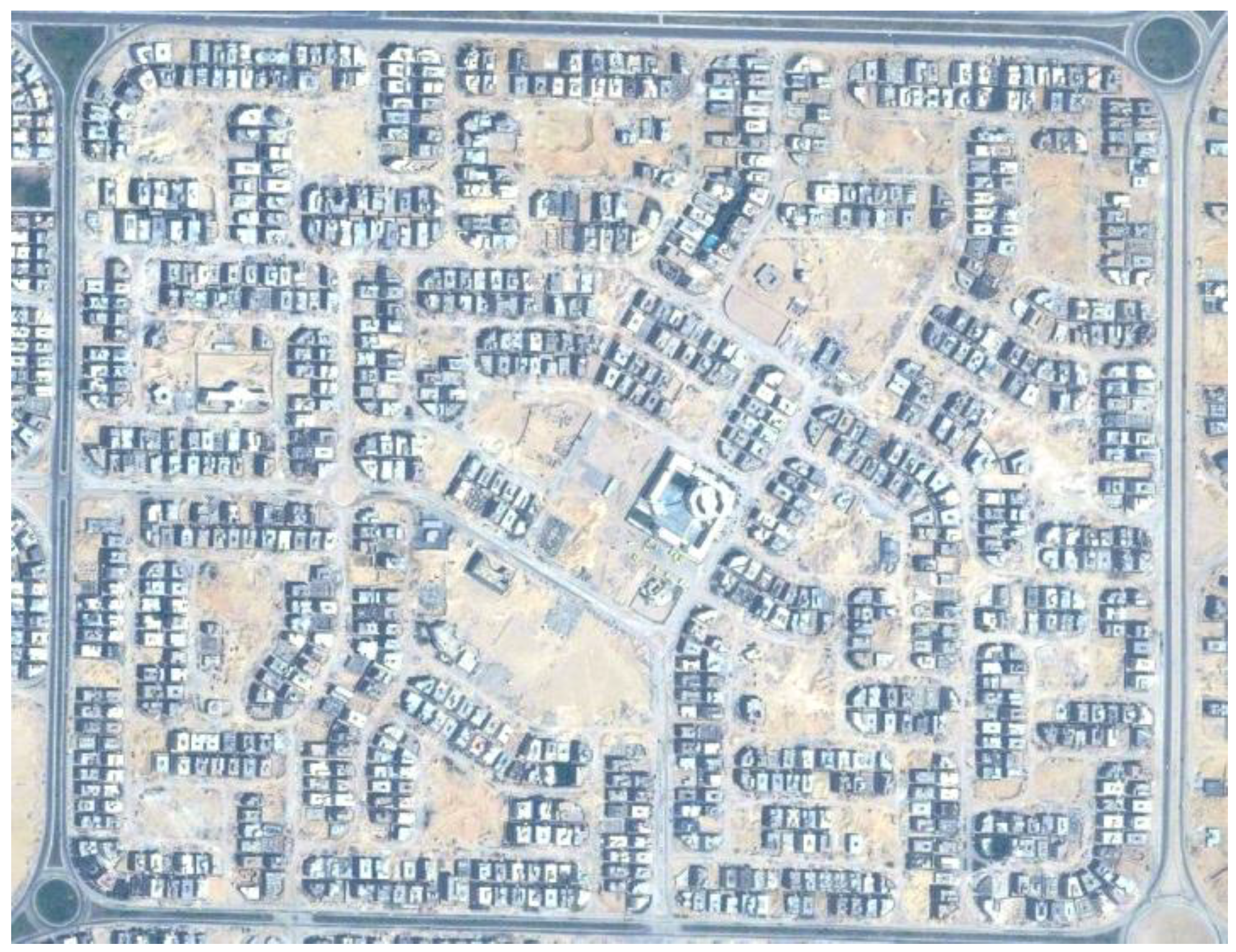
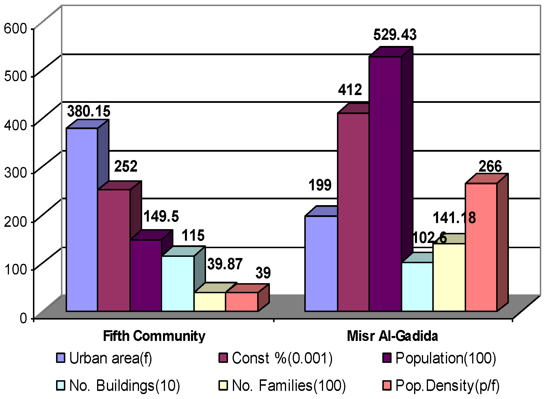
2.3.1. Case 1, the Fifth Community

Fifth community is part of New Cairo suburban developments. Its area is about 5–6 neighborhoods in scale of which the 3^rd district is considered case1 (Figure 2). It is located to the east of the 1st Greater Cairo’s ring road at 50 m above Al-Moqatam Mountain. New Cairo was planned as one of new towns’ series around Cairo to attract population from metropolitan areas. Although it was planned as rural traditional neighborhood development, it turned into automobile dependent suburban sprawled development, the matter that increased the load on metropolitan Cairo [59,60]. Calculations from CAPMAS [61] databases give an impression of the existing population of the site considering the Egyptian family of 3.75 persons in average, based on the latest national population surveys of Egypt [61]. The dominant housing typology is ground plus two floors single family, where the construction regulations defined a dot fabric urban planning pattern. Amongst these regulations; setbacks from all plot area sides leads to 50% Floor Area Ration (FAR) of the plot area [62], and hence leads to the dominant dot pattern of the site.

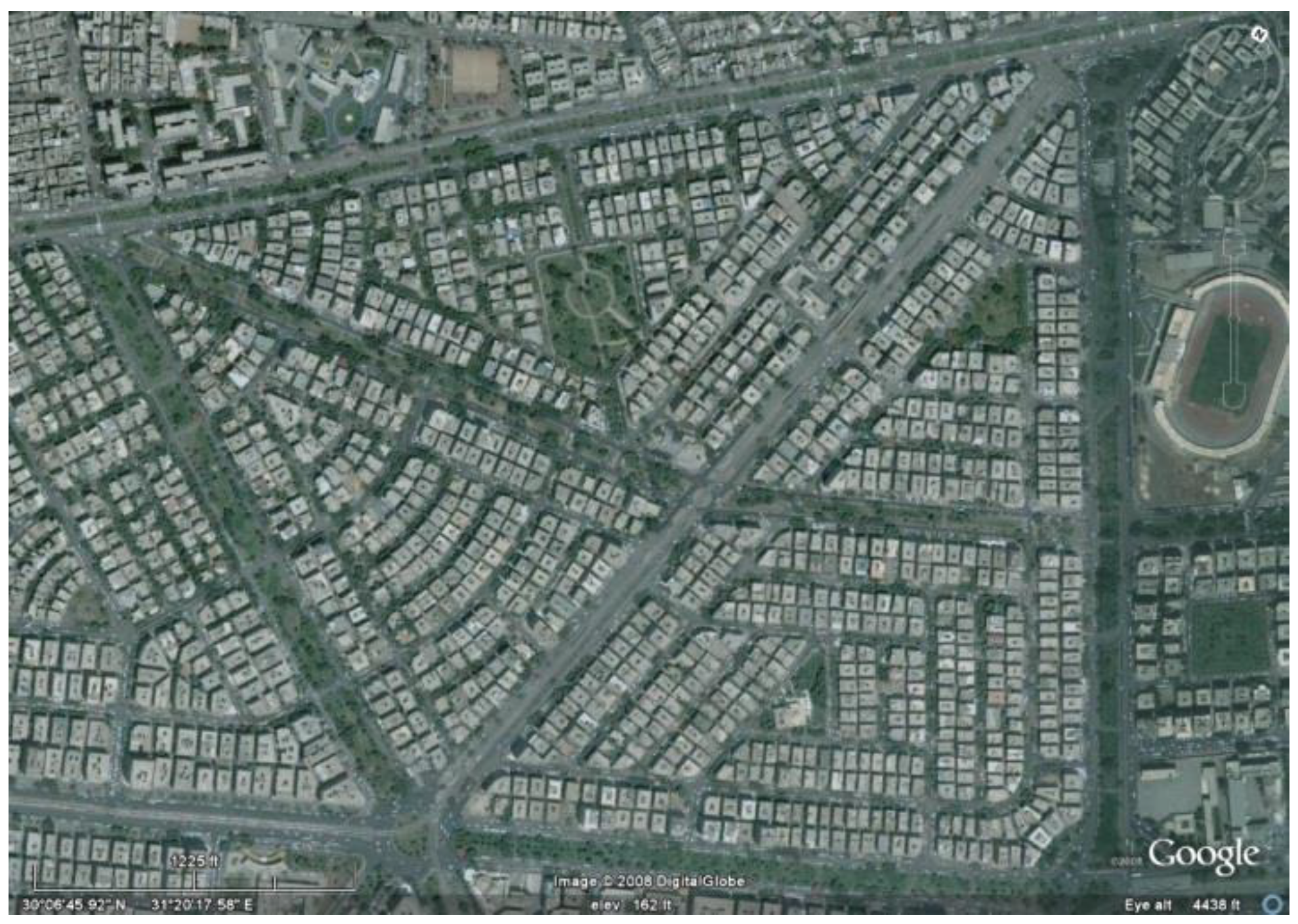
2.3.2. Case 2, Misr Al-Gadida

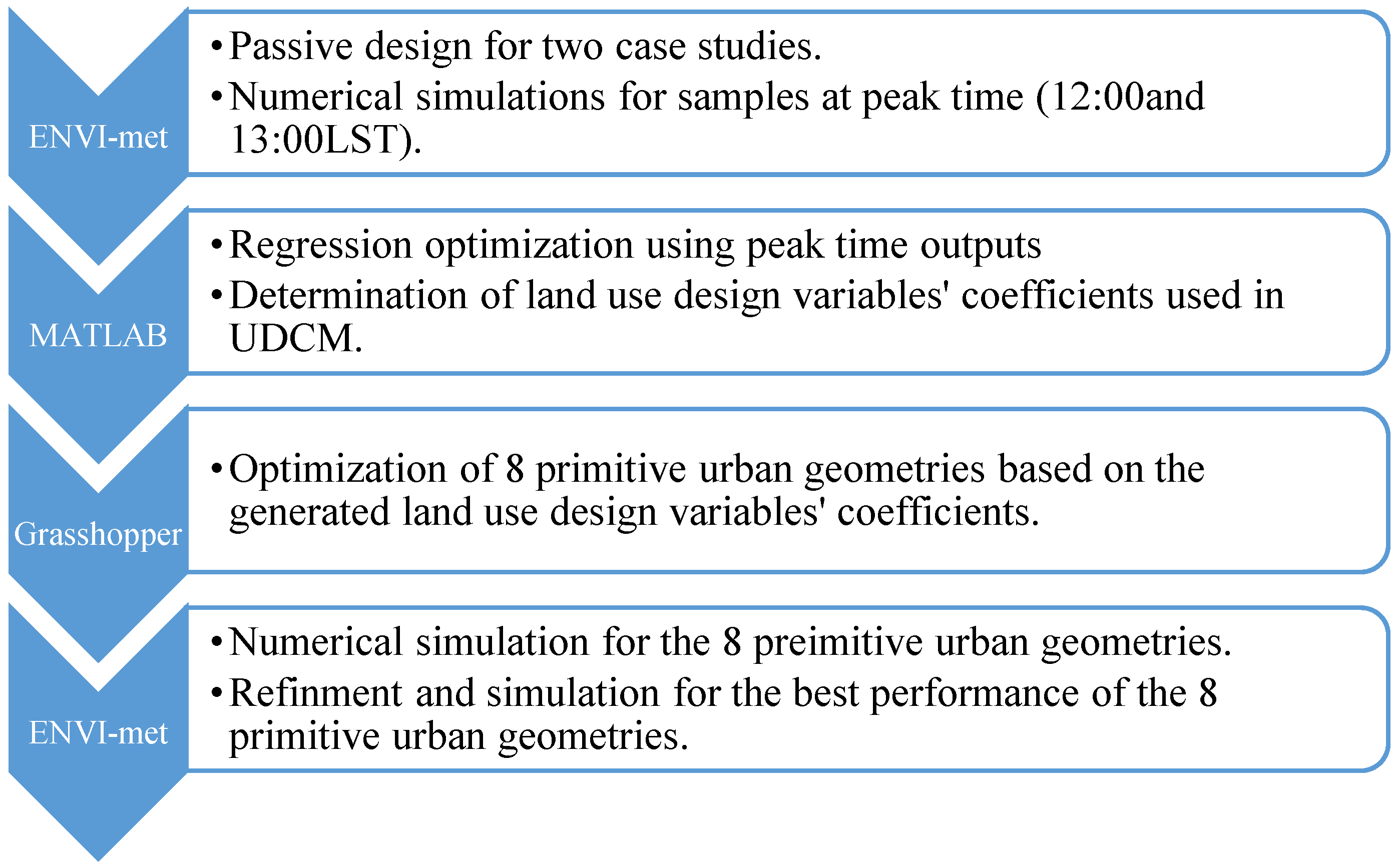
Misr Al-Gadida was built in the early 20th century as a development for the housing suburb located to the northeast of metropolitan Cairo over about 18,000 feddans near the place of ancient Heliopolis (Figure 3) [63]. The feddan area (feddan = about 4200 m²) unit had to be used as an obligation from the Egyptian urban planning law and its amendments in 2007. Misr Al-Gadida mixed uses improved its urban form by time and attracted more population to reveal different housing typologies. Comparisons of site population calculations for the two case studies of this research are based on about 120 m²/flat/dwelling as an average between the medium and upper classes of flat housing areas with 3.75 people/family (Figure 4) [61].

3. Methods

3.1. Numerical Simulation Tool

Assessment of urban design environmental impacts is important for sustainability accreditation of urban comfort. Such approach has been presented by Michael Bruse [3] using ENVI-met for thermal effects in a limited urban area. Bigger scales necessitate considering the complex environmental details which lead to using the numerical assessment methods to distinguish between different master plans. Among the many models in the field of urban climatology to account for urban environmental interactions, ENVI-met is capable of assessing human thermal comfort, predicting all meteorological parameters and all urban surfaces and vegetation thermal interactions sufficiently [17,18,19,28,64]. In order to assess both whole sites as a first step of optimizing a design-based urban form in favor of pedestrian thermal comfort, simulations of both base cases and suggestions were applied. It is meant here by suggestions the regression samples considering the integration of passive applications to the existing site cases. Simulations were held for 12 h from 6:00–18:00 local solar time (LST) on the 1st of July as a representation for the extreme summer day analyzed by ECOTECT v.5.6. Results were recorded at 1.6 m height all over the model area to represent a pedestrian thermal comfort point of view. Thermal comfort in this work is calculated by ENVI-met in terms of the Physiological Equivalent Temperature (PET) which accounts for the meteorology and biometeorology affecting a pedestrian in significant terms [65].

ENVI-met has been validated through many studies to proof its reliability for usage in urban microclimate research and proved an acceptable validity for many meteorological variables [66,67]. Herein this study, ENVI-met has been validated via both air temperature and the mean radiant temperature at the authors’ department of architecture by comparing field measurements and receptor simulation results at the same field point (Figure 5). The HOBO-U30 weather station [68] was used to measure Ta, RH, and V, while the Extech Heat Stress WBGT Meter [69] was used to measure the radiant temperature at the same specific point of the receptor placed in ENVI-met model. The measured data entry used in ENVI-met was on the 5th of August 2017. Figure 6a,b indicate the comparison results of ENVI-met against field measurements and their R² relation for air temperature, whereas Figure 7a,b indicate their comparison and R² relation for radiant temperature.

Air temperature comparisons showed a difference of 1.6 °C at 12:00 LST in favor of field measurements. The calculated R² gave 0.983 for the relation between air temperature resulted from ENVI-met and field measurements at the receptor point. Radiant temperature comparisons showed a difference of 6.3 °C at 09:00 LST in favor of ENVI-met results and the least difference was 1.9 °C at 08:00 LST in favor of field measurements whereas the difference recorded 2.8 °C at the solar altitude peak time (13:00 LST). The calculated R² recorded 0.903 for the relation between radiant temperature plots of ENVI-met and field measurements at the receptor point. The results of these comparisons broadly support ENVI-met to be used as a reliable tool for the research simulations.

3.2. Optimization Tools

3.2.1. Optimizing Design Parameters Coefficients for Pedestrian Comfort

MATLAB [70] is a numerical software that has become the de-facto tool for scientific computing. It has a multitude of pre-programmed numerical recipes and it can also be tailored for any required custom task [71]. In this work, MATLAB has been applied for; visualization of the simulation results obtained from the previous step; regression analysis and; finally for optimization.

3.2.2. Optimizing Urban Form Geometry for Pedestrian Comfort

After getting the design parameters coefficients, Grasshopper has been applied for the optimization of the urban form geometry based on those prescribed coefficients. Grasshopper is a visual programming environment-developed at Robert McNeel & Associates—that works as a—tightly integrated-graphical algorithm editor for Rhinoceros, the 3D modelling, analyzing, and rendering software [72]. Rhinoceros, can use Non Uniform Rational B-Spline (NURBS) shapes, geometries, and point cloud, to generate highly complex and accurate 3D models from simple shapes and curves [73]. Joining Grasshopper with Rhinoceros could refine most of advanced applications of architecture and urban design by generating complex parametric geometries and models [73]. This means that designers once established the relationships that generate a design model, could manipulate it by editing these relationships instead of directly editing the model itself. Consequently, Grasshopper increases the flexibility of computational form finding, and the ability to explore different design iterations by avoiding to directly remodel the design at every turn. In order for the process of relationship definition to be parametrically designed, an additional concept of design thinking is required. As a step backward from the direct design process, the focus of this concept is to logically connect the design parts together which requires a complex act of thinking of new skills and strategies [74].

4. Urban Form Passive Design

In this work; BC stands for base case, DS1 stands for design suggestion no.1 and DS2 for design suggestion no.2.

4.1. Fabric

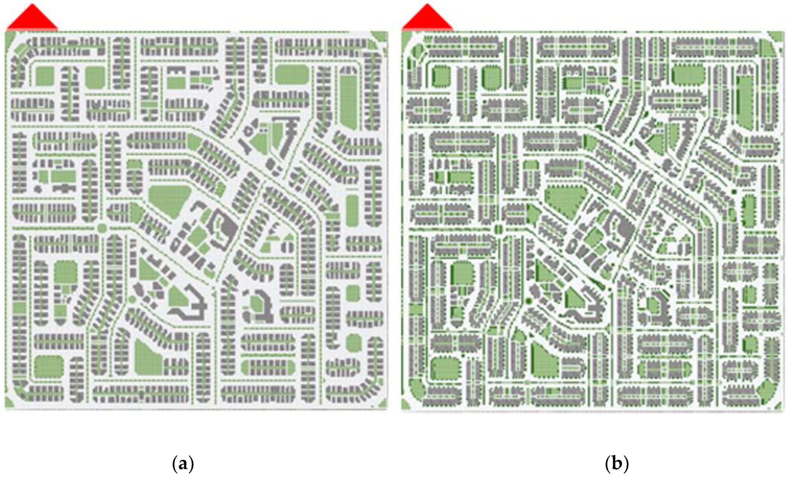
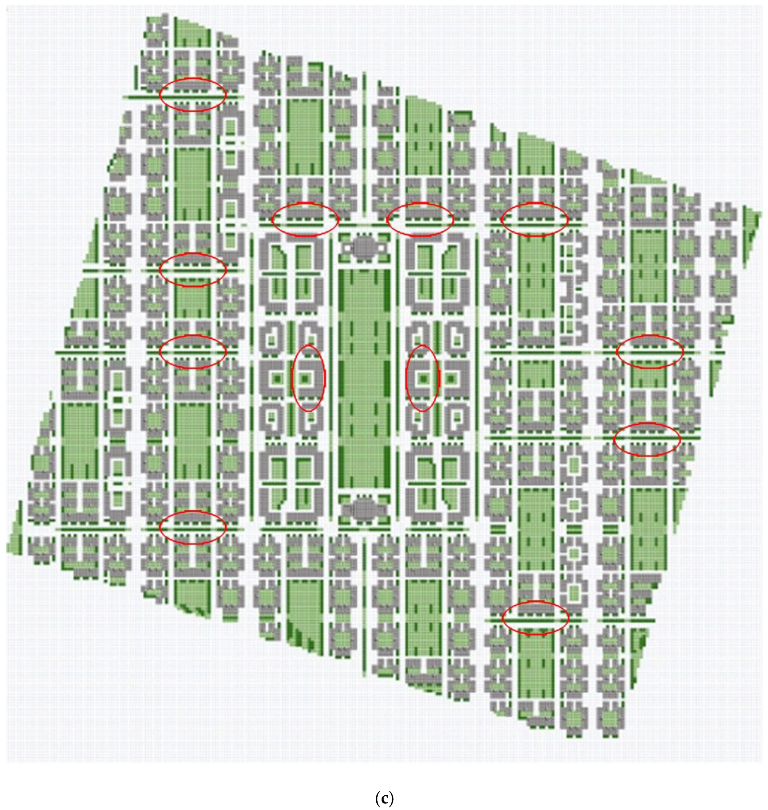
• In both cases there were two alternatives compared with the base case. Alternatives offer different housing types with more responsive clustered form, green coverage, and urban trees arrangements. This medium population-based hybrid form design resulted in different degrees of compactness (D_c). Figure 8 and Figure 9 show master plans and the clustered fabric used for the base case and the suggestions. The modifications which took place for the cases are theoretical; they have been made just for the research purposes where; DS1 is a clustered urban form planned over the same BC zoning in order to study the effect of only the clusters and; the DS2 of both cases are planned on a new zoning and network. With ground and three typical floors (G+3), all housing units are either single flat of 150 m² or duplex of 300 m², designed with 150 people/feddan population density limit of [75] and the 3.75 people/family of [61]. DS1 zoning and land use percentages are the same as BC whereas DS2 with completely new zoning is having merely the same land uses percentage of services.
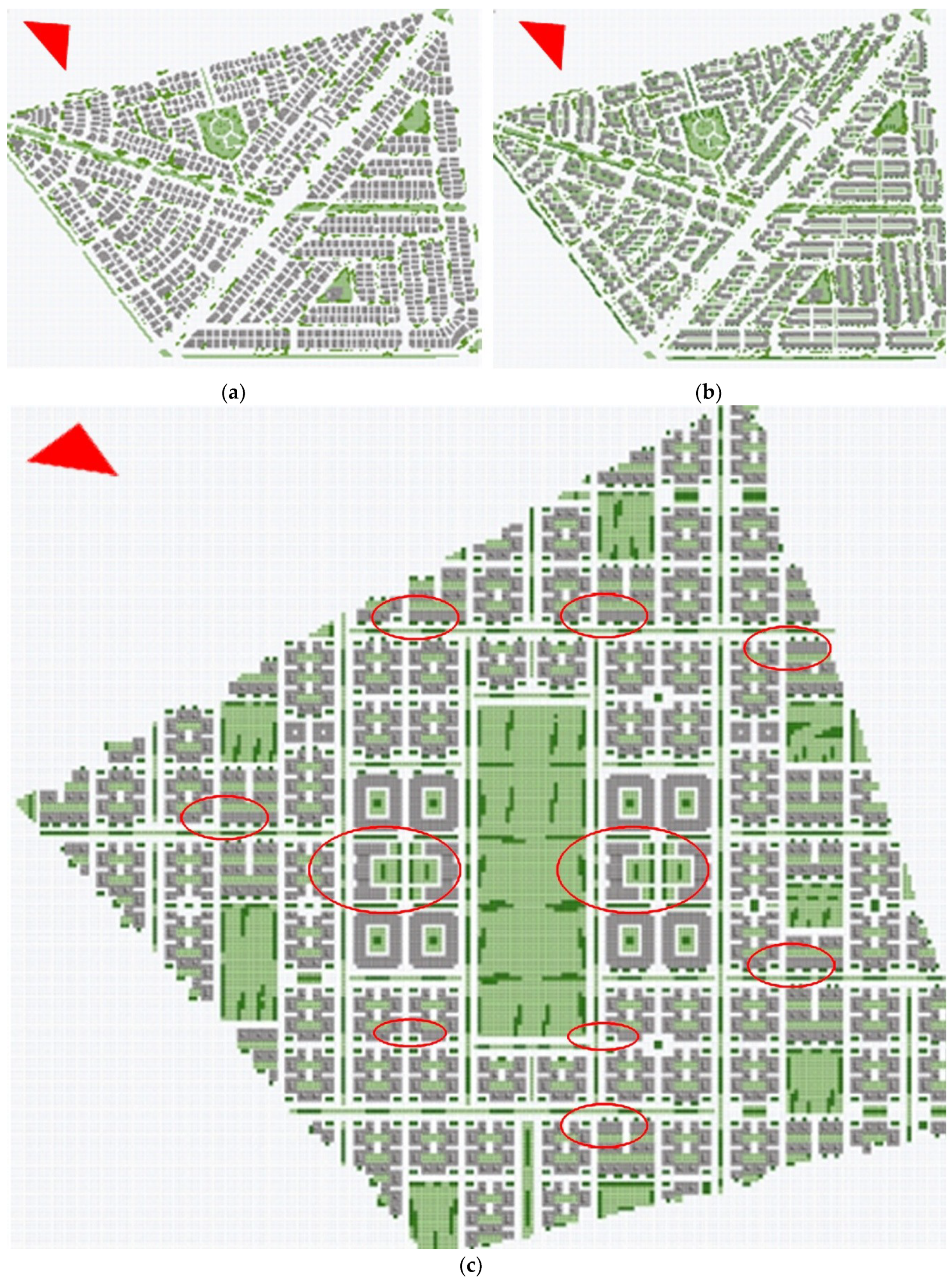
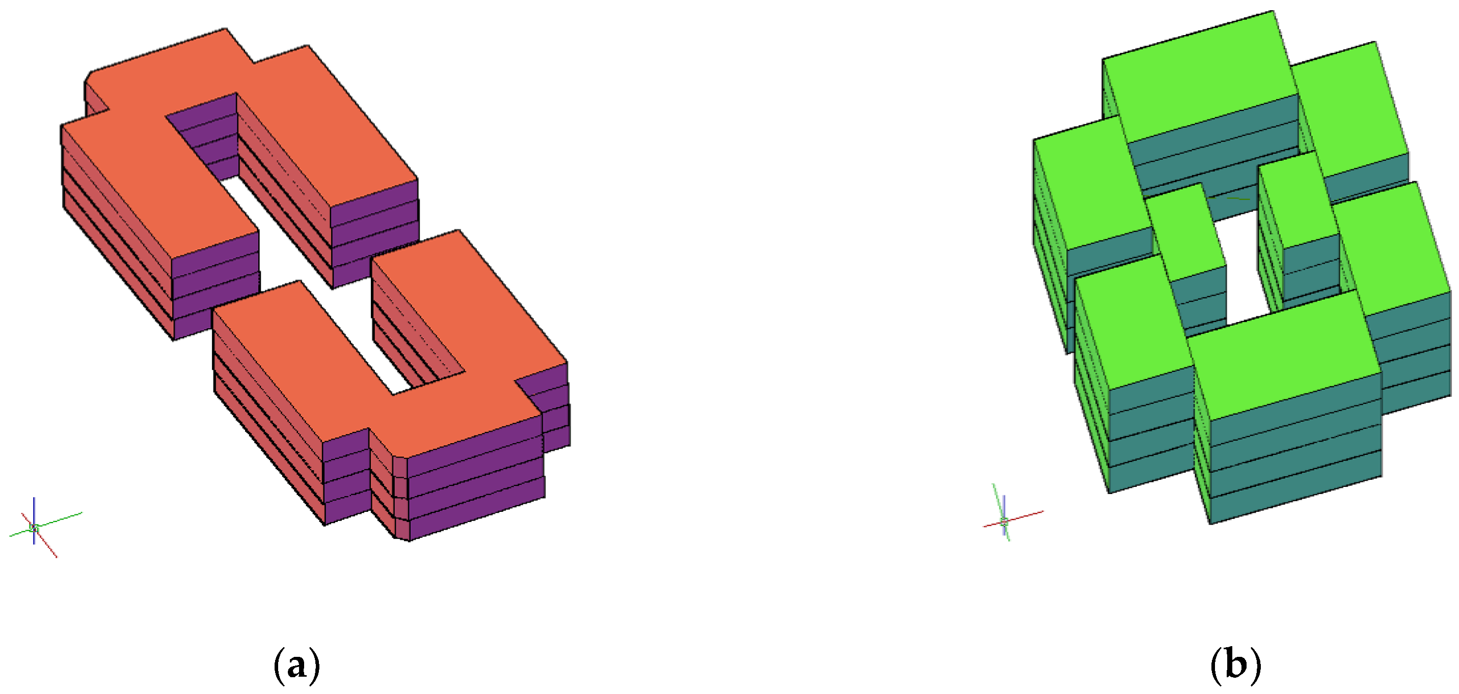
• DS2 clusters is designed to have 1:3:1.3 aspect ratio for W/L/H [76,77], and almost all clusters’ courtyards are oriented 15° from east-west axis following [20]. The canyons’ axes are either same orientation or perpendicular towards north-west to catch prevailing wind and to help the tunneling cooling effect. Figure 10 illustrates the clusters used.
• Following the wind implications on the aspect ratio concluded by Oke [1] and Santamouris et al. [78], DS2 of both cases’ N–S canyons have H/W equal to 1, whilst only collectors or distributors are having H/W equal to 2/3.
• While the network patterns was hierarchical gird and hierarchical radial for BC1 and BC2 respectively, it was transformed to gird in both cases C1DS2 and C2DS2 to allow as much tunneling effect as possible.

4.2. Urban Vegetation

1. The GreenSect concept has been applied following [12,79]. Distances between each two public GreenSect places are described bio-meteorologically upon human walking speed, and the maximum distance can be walked in a neighborhood as an urban planning rule. In this work, it is about 600 m as an intermediate distance between the 300 m of the regulatory agency of English Nature standards and the 900 m (15 min walking) of the European Environmental Agency recommendation of access to green space [12,79], knowing that Duany [80] described the 5 min walking as the basis for the traditional neighborhood development.

2. Urban trees were arranged so that the sheltering effect could decrease time of exposure to solar radiation to a minimum. Urban trees used in this research (

Table 1. Abbreviations used for trees.

Abbreviation	Meaning
T0	No Trees; the base case situation of site one
TE1	Ficus Elastica (Indian rubber plant), with LAI = 1.
TE2	Peltophorum Pterocarpum (Yellow Poinciana), with LAI = 1.
TE3	Ficus Nitida, with LAI = 1.
TC1	Ficus Elastica (Indian rubber plant), with LAI = 3.
TC2	Peltophorum Pterocarpum (Yellow Poinciana), with LAI = 3.
TC3	Ficus Nitida, with LAI = 3.

) have been modeled in both cases following the methodology described by Fahmy et al. [28].

5. Results of UDCM Proposals

5.1. UDCM Derivation from Microclimatic Samples’ Simulations

After assessing the different urban form designs, it’s worth thinking how an urban planner can start practicing on a climate basis for a specific location. Therefore, as the calculated comfort from simulations compiles all built environment responses to microclimate, a regression Urban Design Comfort Model (UDCM) for the cases’ output PET has taken place to account for all meteorology that affect pedestrian comfort such as the relative humidity and wind speed [81].

The local scale compactness, percentage of green coverage, and the urban network area percentage are the main parameters that compose a land use for an urban area. Hence, an approach to investigate how local climate can be useful for urban planners and neighborhood development in terms of the local mean PET value is presented by the following composition. The parameter PET is used to equal the left hand side of the empirical equation whose right hand side is composed of the design parameters (land use and population density) that revealed the PET on the left hand side. Increasing D_c was in terms of one more floor which is named as shown in (

Table 2. Housing design and land use statistics used in modeling in ENVI-met.

	Case Name	Urban Area in Feddans	Green Coverage %, Ag	Tree Type, Tp and Lm	Cluster Closure Ratio;	Cluster Aspect Ratio; H/W/L	Urban Fabric %, Ac	Average no. of Site Floors, nf	Degree of Compactness, Dc	Total Population in Persons	Population Density in p/f
1	BC1	380.15	0.368	TE3, 0.022, 0.62	------	------	0.252	3.171	0.799	14,950	039
2	C1DS1		0.291	TE1, 0.146, 0.138	various	various	0.299	3.911	1.169	46,662	123
3	C1DS1_Dc		0.291	TE1, 0.146, 0.138	various	various	0.299	4.610	1.378	55,004	145
4	C1DS1_Lm		0.291	TC2, 0.146, 0.285	various	various	0.299	4.610	1.378	55,004	145
5	C1DS2		0.476	TC1, 0.145, 0.414	3.47	1:1.3:3	0.310	4.077	1.264	50,448	133
6	C1DS2_Dc		0.476	TC1, 0.145, 0.414	4.27	1:1.6: 3	0.310	4.968	1.540	61,473	162
7	C1DS2_Lm		0.476	TC2, 0.145, 0.285	4.27	1:1.6: 3	0.310	4.968	1.540	61,473	162
8	BC2	199.0	0.105	TC3, 0.123, 1.86	------	------	0.412	4.920	2.027	52,943	266
9	C2DS1		0.273	TC1, 0.077, 0.414 + TC3, 0.111, 1.86	various	various	0.327	4.006	1.310	27,372	138
10	C2DS1_Dc		0.273	TC1, 0.077, 0.414 + TC3, 0.111, 1.86	various	various	0.327	4.845	1.584	33,104	166
11	C2DS1_Lm		0.273	TC2, 0.188, 0.285	various	various	0.327	4.845	1.584	33,104	166
12	C2DS2		0.465	TC1, 0.125, 0.414	3.47	1:1.3:3	0.318	4.296	1.366	28,545	143
13	C2DS2_Dc		0.465	TC1, 0.125, 0.414	4.27	1:1.6: 3	0.318	5.237	1.665	34,798	175
14	C2DS2_Lm		0.465	TC2, 0.125, 0.285	4.27	1:1.6: 3	0.318	5.237	1.665	34,798	175

In each abbreviation; letter C stands for case, BC for base case and DS for the design suggestion. T_p and L_m stands for the tree urban coverage and its max. LAD; No. of people/ family is calculated as 3.75 [61]. In all design alternatives except base cases, no. of family flats is also calculated as 150 m²/flat/family. Floor height as 3 m. (Feddan = 4200 m².); Facilities buildings at service civic center are 10 m in both C1DS1 and DS2 whereas 13 m in both C2DS1 and DS2 to increase the compactness degree without increasing site population assuming that more facilities are needed; The actual residential land use can be calculated after extracting 33% for the network and green coverage as [75] tells, also after extracting the civic buildings areas; For UDCM comfort model purposes, suffix D_c in the case name means more compactness. For example, C2DS1 has 13 m height residential buildings, C2DS1_Dc applies 16 m instead. For C2DS1_L_m means using tree TC2 with LAI = 3, instead of using tree TC1 or TC3 of also LAI = 3.

and

Table 3. Samples of Urban Design Comfort Model (UDCM) regression model.

No	Samples	Output Time (LST)	(PET)	Dc	As	Ag (%)	Tp	Lm
1	C1BC	12:00	48.9	0.799	0.380	0.36757	0.022	0.620
2	C1BC	13:00	49.1	0.799	0.380	0.36757	0.022	0.620
3	C1DS1	12:00	46.9	1.169	0.392	0.29117	0.146	0.138
4	C1DS1	13:00	47.0	1.169	0.392	0.29117	0.146	0.138
5	C1DS1_Dc	12:00	45.0	1.378	0.392	0.29117	0.146	0.138
6	C1DS1_Dc	13:00	45.2	1.378	0.392	0.29117	0.146	0.138
7	C1DS1_Lm	12:00	44.7	1.378	0.392	0.29117	0.146	0.285
8	C1DS1_Lm	13:00	44.7	1.378	0.392	0.29117	0.146	0.285
9	C1DS2	12:00	44.7	1.264	0.214	0.47620	0.145	0.414
10	C1DS2	13:00	45.4	1.264	0.214	0.47620	0.145	0.414
11	C1DS2_Dc	12:00	44.0	1.540	0.214	0.47620	0.145	0.414
12	C1DS2_Dc	13:00	44.7	1.540	0.214	0.47620	0.145	0.414
13	C1DS2_Lm	12:00	43.9	1.540	0.214	0.47620	0.145	0.285
14	C1DS2_Lm	13:00	44.7	1.540	0.214	0.47620	0.145	0.285
15	C2BC	12:00	47.9	2.027	0.483	0.10471	0.123	1.860
16	C2BC	13:00	49.7	2.027	0.483	0.10471	0.123	1.860
17	C2DS1	12:00	42.3	1.310	0.40	0.27299	0.188	1.267
18	C2DS1	13:00	44.4	1.310	0.40	0.27299	0.188	1.267
19	C2DS1_Dc	12:00	44.7	1.584	0.40	0.27299	0.188	1.267
20	C2DS1_Dc	13:00	44.9	1.584	0.40	0.27299	0.188	1.267
21	C2DS1_Lm	12:00	44.6	1.584	0.40	0.27299	0.188	0.285
22	C2DS1_Lm	13:00	44.6	1.584	0.40	0.27299	0.188	0.285
23	C2DS2	12:00	43.2	1.366	0.217	0.48576	0.125	0.414
24	C2DS2	13:00	44.0	1.366	0.217	0.48576	0.125	0.414
25	C2DS2_Dc	12:00	44.3	1.665	0.217	0.48576	0.125	0.414
26	C2DS2_Dc	13:00	44.6	1.665	0.217	0.48576	0.125	0.414
27	C2DS2_Lm	12:00	44.3	1.665	0.217	0.48576	0.125	0.285
28	C2DS2_Lm	13:00	44.4	1.665	0.217	0.48576	0.125	0.285

In all cases’ names; D_c stands for the increased compactness from the previous case no. whereas L_m stands for a different tree from the previous case no.

). A point of view of urban form design parameters considers the number and types of trees used as also responsible of generating a specific level of local mean comfort. Therefore, the maximum leaf area density (LAD) value, L_m, is used to represent a specific urban tree whose built grids in ENVI-met model area can be counted and then represented as Tree Plantation area T_p. After all, this design composition can be empirically represented by an equation summing the form design parameters as following:

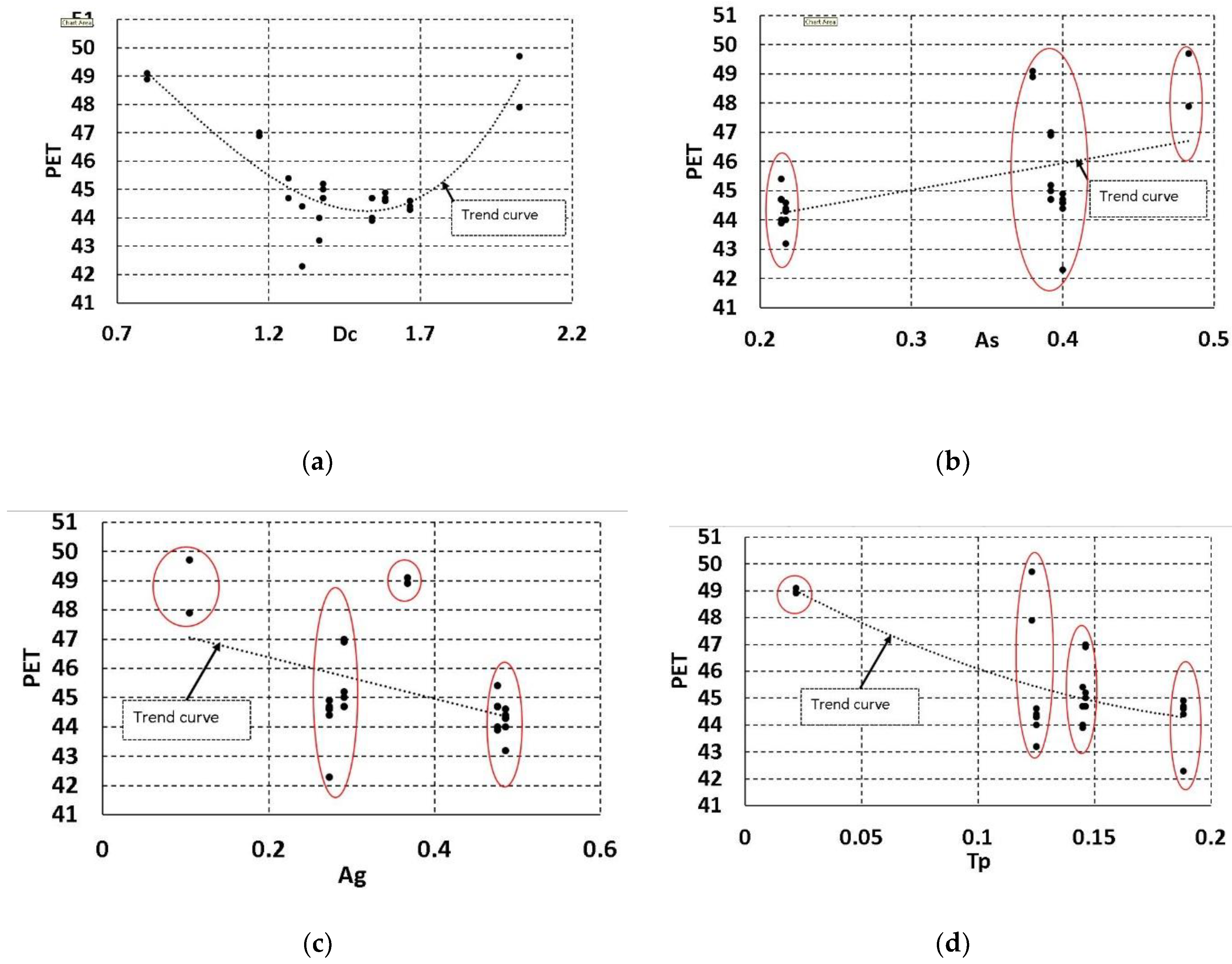
• D_c standing for fabric volume, i.e., residential construction percentage (A_c) × canopy layer height, or the number of urban floors (n_f) which in turn can be calculated from the population.
• A_c is the urban site constructed area percentage.
• A_g is the green coverage area percentage.
• A_s is the urban asphalt network area percentage.
• T_p represents the urban trees shadow coverage with a specific tree. T_p is the trees’ grids percentage compared with the site outdoor grids built in ENVI-met model which give an indication for the urban shadow produced at peak time generated by trees.
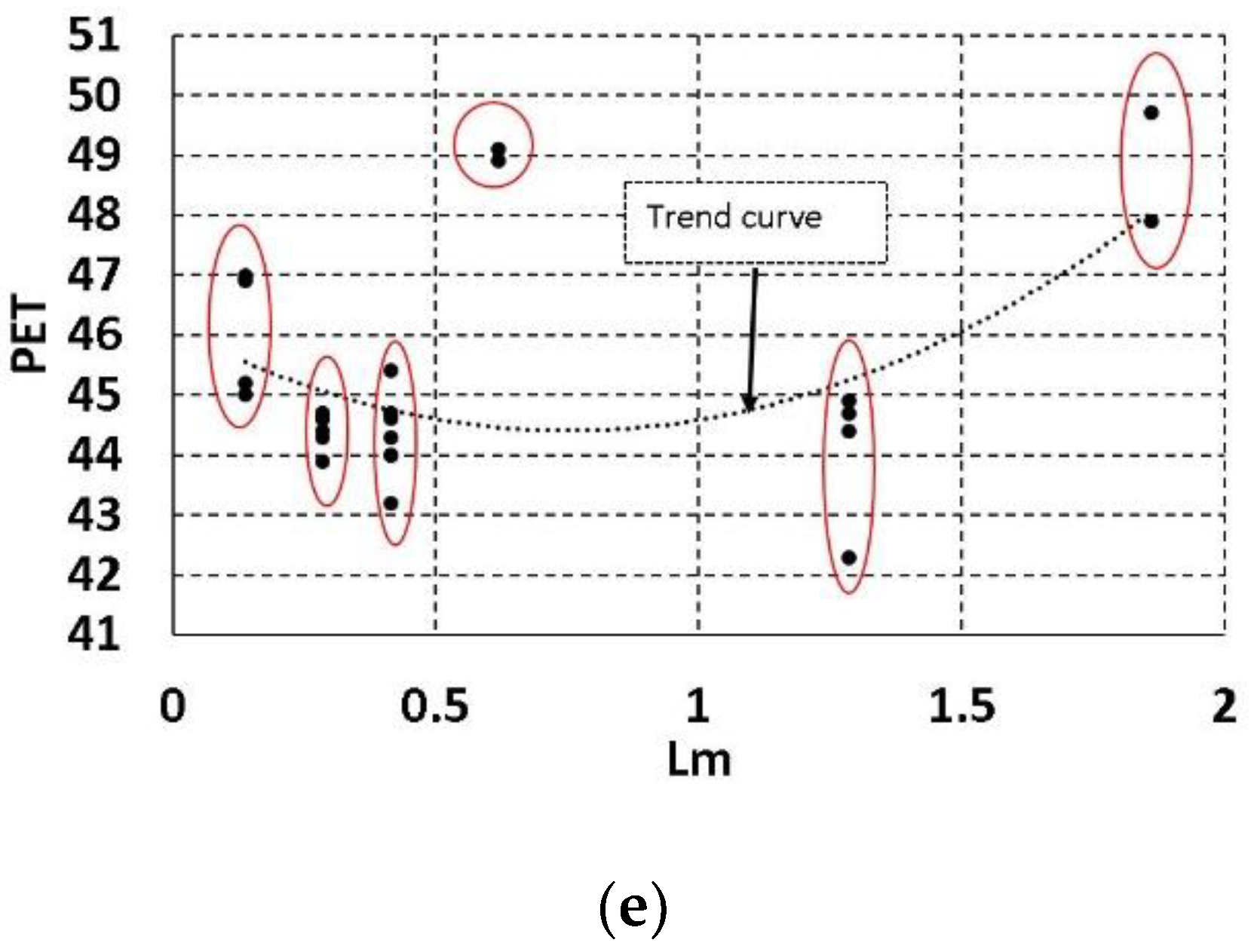
• L_m is the site mean maximum LAD of the tree—as quantification for the type of trees used in the site—to represent the effect of specific urban trees on the local comfort.
• n_f is the urban site average floor number which is needed to calculate the site compactness degree.

Thus, an initial equation can be empirically written to represent the land use parameters that compose an urban passive system as following:

$$UDCM=c_1.A_c+ c_2. A_g+ c_3. A_s+ c_4. T_p+ c_5. L_m+ c_n$$

(1)

where UDCM is the urban comfort level at a time in terms of PET. Percentage of trees coverage applied along with fabric in each BC and DS is shown in (Table 2).

Table 3 shows PET comfort levels extracted for design parameters of C1 and C2 master plans at the peak period 12:00 LST and 13.00 LST. The reason of selecting these two peak hours only is that the methodology of modeling urban trees after Fahmy et al. [28] has been empirically derived at peak time of mid-latitude sites. In addition, ENVI-met overestimations do obstruct comfort prediction by night, therefore only the durinal 12 h in summer of a mid-latitude location like Cairo has been simulated as presented earlier. Further, the records for mean PET at the peak time were selected in the regression step to generate the model coefficients, which will theoretically—if solved later—generate land use parameters to cope with the peak climate conditions. In order to increase the samples for the regression to take place from a statistical point of view, an increased degree of compactness and different types of urban trees in terms of L_m for each case have been simulated (Table 3).

According to the Egyptian planning law and the environmental guide for urban spaces [75,82], the basic design parameters, D_c, A_s, A_g, T_p, and L_m with a maximum value of 2 according to the trees modeled and simulated in step 1, which have been used to represent the MATLAB optimization inputs for coefficients derivation are all illustrated in (

Table 4. Initial optimization ranges of UDCM parameters, [75,82].

		Dc	As	Ag	Tp	Lm
1	Urban heart	5.0–8.0	0.15–0.45	0.10–0.30	(0.10–0.6) of (As + Ag)	0.10–2.0
2	Urban center	2.8–5.0
3	Urban core	1.6–3.0
4	Sub urban	0.4–1.8
5	Rural reserve	0.3–0.5

).

5.1.1. MATLAB Optimization for UDCM Model

The main objective of this research is to find the optimum conditions to achieve the most comfortable and feasible environment for inhabitants in an urban environment. This is achieved by applying numerical optimization on a data-driven model that was developed using regression analysis. However, the quality of the optimal solution depends on the quality of the model. Therefore, sufficient effort was performed to develop the most possible reliable model. The process included several steps starting by data inspection and visualization.

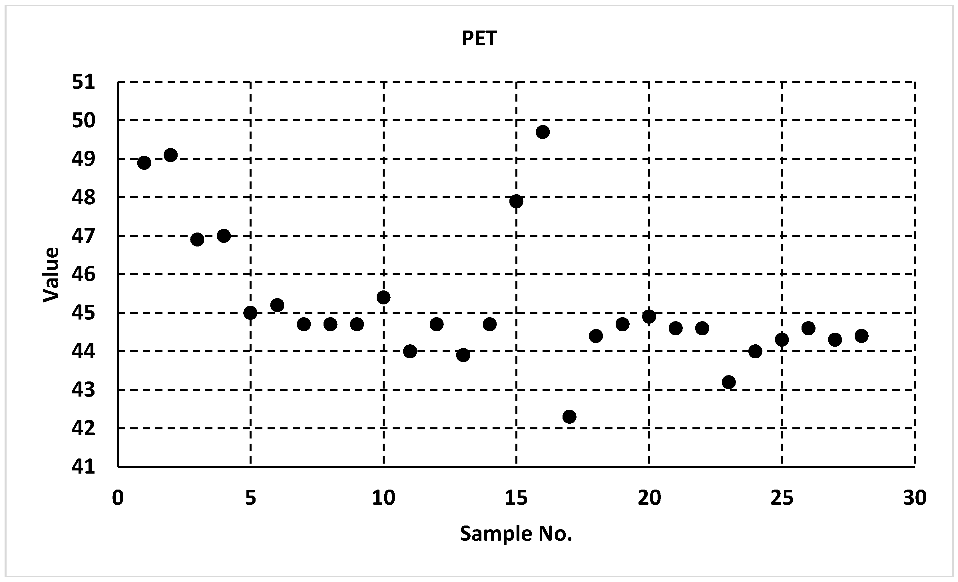
Data Inspections and Visualization

In this section, data in (Table 1) has been investigated before building the regression model. The Table presents 28 rows of sampled data, where D_c, A_s, A_g, T_p, and L_m are the input model variables and PET is the output response. A useful and simple method to investigate the data is to plot the data as shown in (Figure 8). It shows the distribution of PET over a relatively high physiological equivalent temperatures range (42:50). This is predictable because the data was collected during the hot Cairo summer between 12:00 and 13:00 LST, which poses a limit on the forecasting capabilities of our regression model.

Curves are approximately fitted between the data points in each of the sub-plots in (Figure 11). The next step is to examine the relationship between the response (PET) and each of the individual input variables as shown in (Figure 12). They show the trend of the relationship between PET and each of the input variables. This gives an estimate about the impact of each input variable on the variation of PET values. It could be noticed that except for D_c, other input variables are concentrated around three or more discrete values. In addition, the proportional effect of D_c on PET is not clear, however, omitting the first two sample points, could reveal that as D_c increases, PET also increases. It could also be noticed that each A_s and L_m has a positive correlation with PET where A_g and T_p have a negative correlation. However, these are merely preliminary observations since we are only inspecting individual relationships between each variable and PET, and the interaction effects between each pair of variables on the value of PET has not been inspected yet. In general, the relationship between PET and the input variables is complex. Microclimatic change includes numerous mutual effects between built environment elements, fabric, network and vegetation especially in outdoor climate. This must be taken into consideration when developing the UDCM model.

Developing UDCM

This step is of great importance since the model will be used in optimization and it must be ensured that the results are credible and reliable. In this step, linear regression [83] was utilized to develop the model. In its simplest form, a linear regression model fits a line in the form $\tilde{y}=a_{0}x+a_1$, where $a_0$ and $a_1$ are coefficients determined based on the input data. For multi-variant data, the model becomes a hyper-plane in the n-dimension, where n is the number of input variables. One common form of the model is the quadratic model, $\tilde{y}=a_0+a_i{x}_i+a_{ij}{x}_i{x}_j+a_{ii}{x}_i{}^2$, which includes $x_i{x}_j\mathrm{and} x_i{}^2$ terms to account for nonlinearity and curvature in the relation between y and x.

Here, four different types of models were used:

• Linear in the form of: $\mathrm{PET} = 1 + D_c + A_s + A_g + T_p + L_m$
• Interaction in the form of: $\mathrm{PET} = 1 + D_c + A_s + A_g + T_p +L_m+ D_c\ast A_s + D_c\ast A_g + D_c\ast T_p +D_c\ast L_m + A_s\ast A_g + A_s\ast T_p + A_s\ast L_m + A_g\ast T_p + A_g\ast L_m +T_p\ast L_m$.
• Quadratic in the form of: $\mathrm{PET} = 1 + D_c + A_s + A_g + T_p +L_m+ D_c\ast A_s + D_c\ast A_g + D_c\ast T_p +D_c\ast L_m + A_s\ast A_g + A_s\ast T_p + A_s\ast L_m + A_g\ast T_p + A_g\ast L_m +T_p\ast L_m+ D_c^2 + A_s^2 + A_g^2 + T_p^2 +L_m^2$.
• The fourth type is based on the stepwise algorithm [83], where the algorithm starts with one model form -in our case, it is linear- and iterates through adding $x_i{x}_j\mathrm{and} x_i{}^2$ terms in order to maximize the prediction capabilities of the final model.

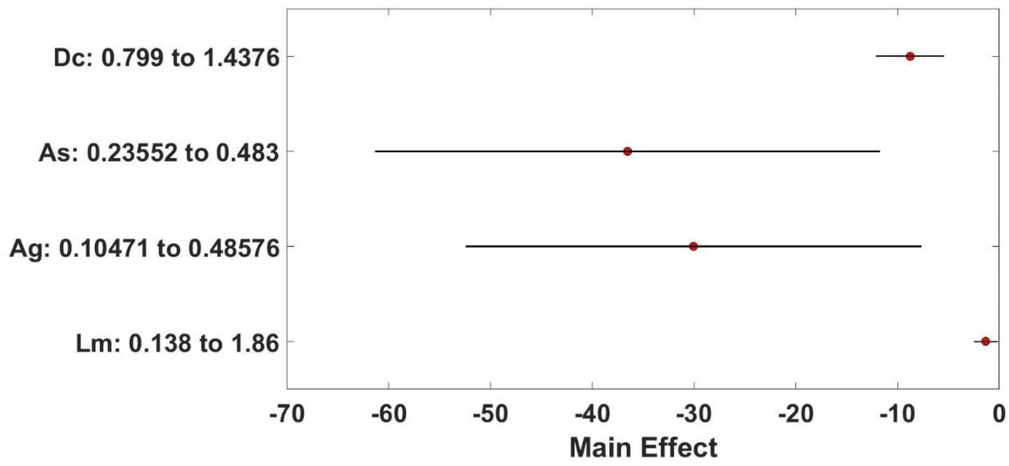
The accuracy and prediction capabilities of the models are judged by the value of ${\mathrm{R}}^2$, which is the coefficient of determination, defined as ${\mathrm{R}}^2=1-\frac{SSE}{SST}$, where, $SSE={\sum }_{i=1}^n{\left(y_i-{\widehat{y}}_i\right)}^2$, and $SST={\sum }_{i=1}^n{\left(y_i-{\overline{y}}_i\right)}^2$ are the summation of errors between true response values and approximate and average ones respectively. When SSE decreases and approaches zero, this means the model fits the data well, and the value of ${\mathrm{R}}^2$ approaches one. However, we must be cautious about over-fitting, by which we mean using un-important design variables in the approximate model. In an extreme case, we can bring the value of ${\mathrm{R}}^2$ to one by using n-1 variables to fit a date of n dimension. To overcome this issue, we use the adjusted ${\mathrm{R}}^2$, which is defined as adjusted ${\mathrm{R}}^2=1-\frac{\frac{SSE}{\left(n-p\right)}}{\frac{SST}{\left(n-1\right)}}$, where p is the number of model variables. This ensures that adjusted ${\mathrm{R}}^2$ only approaches when adding new variables to the model reduces the error between true and predicted values. The values of ${\mathrm{R}}^2$ and adjusted ${\mathrm{R}}^2$ are presented in (

Table 5. Summary of R² and adjusted R² for each model.

Model	R2	AdjR2
Linear	0.81	0.76
Interaction	0.94	0.89
Quadratic	0.94	0.89
Stepwise	0.94	0.92

) for each of the four models. It is clear that the model from stepwise method has the highest values for both ${\mathrm{R}}^2$ and adjusted ${\mathrm{R}}^2$. In addition, both values are relatively near to each other’s compared to other model types. The form is represented as follows:

$$\mathrm{PET} = 1 + D_c + A_s + A_g + L_m + D_c\ast L_m+ D_c^2 + A_s^2.$$

(2)

By comparison, the linear model lacked additional terms to represent the sampled data. This is evident from its low R² value of 0.81 compared to 0.94 for all other models. It can be also noticed that the interaction and quadratic models included some non-significant terms, therefore, the value of adjusted R² decreased as shown. The stepwise algorithm removed these non-significant terms, i.e., removed T_p from the input variables, as it is statistically un-important. However, from physical and engineering points of view, T_p can still be important to PET, as T_p is the tree grid percentage compared with site outdoor grids. The reason that T_p was found to be statistically non-significant to the model, can be due to the limitations on the sampled data. The stepwise algorithm concluded that there is a strong interaction effect between D_c and L_m on the value of PET. It also revealed that D_c and A_s have strong influence on the curvature in the surface of PET. This means that the value of PET changes non-monotonically in the design space and this change is largely dependent on D_c and the interaction between D_c and L_m which represents the tree type. This can be attributed to the increased compactness specifically at the city transect zone urban core (to which the original sample cases belong) where compactness did not allow much tree ground coverage as presented by Morakynio [29] and others. And this probably reveals that a neighborhood case study from each urban transect zone to be included in the initial simulation samples for regression is much representative than two cases. Another reason was the unadjusted T_p ratio in comparison to area of urban spaces in the two cases. The applied T_p in the two cases didn’t exceed 0.188 in C2DS1 and less for the rest of regression samples which revealed independence of the concluded PET on such important physical parameter.

The relative importance of model variables can be visually inspected using the main effects plot as shown in (Figure 13). The x-axis is the value of response PET, where the y-axis represents the change of input design variables. We can see what effect each variable has on the change of PET. The horizontal lines represent the confidence interval on the input variable values. The circle in the middle of the line refers to the number of unit change in PET when a variable changes its value from low to high. For example, when the value of D_c increases from 0.799 to 1.4376, we may expect—with 95% confidence—a decrease in PET by approximately eight units. It is obvious that A_s (asphalt) and A_g (green ground coverage; grass) both have large effect on PET, while L_m has the smallest effect in comparison. However, if the large confidence intervals for A_s and A_g are shrunk and moved to the right side, their relative effect will then be reduced and can approach the same relative effect as D_c and L_m. Based on the results in (Figure 10), we can conclude that all variables have statistically significant negative effect on PET, where A_s and A_g have stronger effects than D_c and L_m.

5.1.2. Optimization

Having a comparatively reliable approximate model developed, we can then use it in optimization. An optimization problem can be formulated as finding the values of D_c, A_s, A_g, and L_m that lower the value of PET to a comfortable value of 24. An additional constraint is added to limit the design space to values within the lower and upper physical bounds on the design variables. The optimization problem can then be written as:

$$Find \left(X_{opt}\right)that:$$

$$\mathrm{PET}-24\le 0$$

$$0.3\le D_c\le 3$$

$$0.15\le A_s\le 0.3$$

$$0.1\le A_g\le 0.3$$

$$0.1\le L_m\le 2.$$

The problem is solved in MATLAB using different algorithms, the active-set, interior-point, and the sequential quadratic programming algorithms. They are gradient-based algorithms, i.e., they depend on calculating the gradient. In addition, two heuristic type algorithms are used: the genetic algorithm and the simulated annealing algorithm. Different initial points were used to ensure that no algorithm would be stuck at a local minimum. The algorithms converged to the optimum values shown in (

Table 6. Optimum values.

Algorithm	Dc	As	Ag	Lm
SQP	1.2083	0.3000	0.3000	1.9649
	1.2084	0.1500	0.3000	1.9645
	1.2307	0.3000	0.3000	1.9733
interior-point	1.2138	0.1500	0.3000	2.0000
	1.2138	0.1500	0.3000	2.0000
	1.2138	0.1500	0.3000	2.0000
active-set	1.2138	0.1500	0.3000	2.0000
	1.2406	0.0871	0.3629	2.0608
	1.2442	0.3729	0.3729	2.0729
simulated annealing	1.2603	0.1500	0.3000	1.7437
	1.1931	0.1500	0.3000	2.0000
	1.1197	0.1662	0.3000	1.8154
GA	0.3010	0.2394	0.1009	0.1015
	0.3001	0.2354	0.1000	0.1000
	0.3000	0.2354	0.1000	0.1000
Average	1.0308	0.1991	0.2691	1.5931

). The average is calculated and presented in the last row. It can be concluded that the algorithms have converged towards the minimum bound for A_s and the maximum bound for A_g and L_m. This agrees with many investigations for the effect of both green coverage and the specific types of urban trees rather than only the ground coverage of those trees when it comes to dense fabric [28,84,85].

5.2. UDCM Validation

5.2.1. Grasshopper Optimization for Urban Form Geometry

UDCM model has been validated through the modeling and simulation of primitive urban forms that have a compactness degree belonging to the central urban area of a city. Those primitive urban forms were eight and have been geometrically generated by Grasshopper using the urban form design coefficients optimized from MATLAB Grasshopper. Figure 14 illustrates the aforementioned eight primitives.

5.2.2. ENVI-met Optimization Results for UDCM

Eventually, the eight primitive urban forms generated from Grasshopper were modeled and simulated numerically in ENVI-met to check how much microclimate can be improved by using optimum values from MATLAB and grasshopper. In a further ENVI-met simulation step for validation, the best form of the ENVI-met simulation among the eight primitives was refined in terms of increased greenery coefficients; i.e., L_m which have an increased effect as shown in Table 6. The refinement was in terms of more dense trees and L_m values from 1.59 as generated from MATLAB to become 2.0729 (the maximum L_m generated from MATLAB) and reflects on rest of tree’s LAD values integrated on the tree canopy height.

In the first sub-validation step of ENVI-met numerical simulations, form no. 7 showed better microclimatic conditions in terms of PET despite microclimate was generally still very hot.

Table 7. Ranges of PET.

PET	Thermal Perception	Physiological Stress
4 °C	Very cold–cold	Extreme cold stress–strong cold stress
8 °C	Cold–cool	Strong cold stress–moderate cold stress
13 °C	Cool–slightly cool	Moderate cold stress–slight cold stress
18 °C	Slightly cool–comfortable	Slight cold stress–no cold stress
23 °C	Comfortable–slightly warm	No cold stress–slight heat stress
29 °C	Slightly warm–warm	Slight heat stress–moderate heat stress
35 °C	Warm–hot	Moderate heat stress–strong heat stress
41 °C	Hot–very hot	Strong heat stress–extreme heat stress

shows the PET ranges [65,81] whereas Figure 15 indicates the PET values calculated by RayMan [86] using ENVI-met meteorological outputs for the refined urban forms. These statistical results from Figure 15 showed an improvement to the hot zone compared to their very hot initial values before refining; which in turn proofs the reliability of the optimized UDCM and its coefficients. For example, the primitive proposal no. 7 recorded a PET value of 38.7 °C at the first step of validation simulation at 12:00 LST and 36.8 °C after refinement with extra L_m. PET values of Opt7 increased again at 13:00 LST where stored heat started to emit afternoon but kept less than even the least values of Opt2 (regular form with four green spots and oriented to the prevailing wind) recording 39.3 °C and 37.3 °C.

6. Discussion and Conclusions

This research rolled around climate-based urban planning in Cairo and its benefits for wellbeing in terms of human outdoor thermal comfort as well as giving an approach to ease the complexity of applying climate knowledge in practice because of its interdisciplinary nature. These two main objectives couldn’t have been approached unless urban passive design in terms of geometrical adjustments and green structure of case studies were presented to know how climate interact passively within a so called, hybrid urban form, in a first set of numerical simulations using ENVI-met.

The data included two different sets: one for the Fifth Community, which consists of mainly single family housing which allow for wind and solar access and on the other hand, Misr Al-Gadida which is over populated with high rise apartment residential buildings limiting both sun and wind access.

Consequently, the proposed hybrid urban form increased population in the first case and vice versa in the second. This is in order to offer a medium population urban form which at the same time offered controlling the local urban climate conditions and the thermal performance as if they were applied instead of the existing forms. By this way, urban passive applications such as geometry adjustments and GreenSect with trees can be to some extent the solution to the lacking connection between climate knowledge and its applied practice. After this platform, two main suggested urban clustered forms with GreenSect were simulated for each case; the first one was built over the existing site zoning whilst the second was a new master plan. The second suggestion for each case is a complete newly designed urban form as if climate was observed when applying a proportionally refined clustered form. Results of PET at peak time using the clustered fabric and the GreenSect were collected as samples for further investigation on how to generate an urban design model on a pedestrian thermal comfort basis that can be used by practitioners in the early stages of sketching and design.

This work included developing a data driven model that was built using sampled data from ENVI-met. The data was first carefully visualized and inspected, then regression analysis was applied. Particular attention was given to the selection of the type of regression model. The stepwise regression model succeeded in representing the data with the highest accuracy. The step-wise algorithm succeeded in creating the best fit of 94% R² and 92% adjusted R². The model revealed that the interaction between D_c and L_m significantly affect the value of PET. In addition, the model showed that D_c and A_s have a significant effect on the variability of PET within the limiting design space. In other words, if the change of PET is represented by a hypersurface in a multi-dimensional space, D_c and A_s highly affect the curvature of this surface.

An important note should be emphasized; although the step-wise model rules that T_p was statistically non-significant, however, an informed decision should consider it physically important. T_p is the tree grid percentage compared with site outdoor grids, therefore, it certainly has an effect of the change of PET. The reason behind this conflict can be attributed to the limited size of sampled data.

And this probably reveals that a neighborhood case study from each urban transect zone to be included in the initial simulation samples for regression is much representative than two cases. Another reason was the unadjusted T_p ratio in comparison to area of urban spaces in the two cases. The applied T_p in the two cases didn’t exceed 0.188 in C2DS1 and less for the rest of regression samples which had to be more up to 0.5 in hot regions, the matter that resulted in the independence of PET on such important physical parameter. Nevertheless, after the third phase of developing UDCM using Grasshopper, the fourth step of simulating such eight proposals showed PET improvements in comparison to the mid-latitude sites at peak time, especially the primitive proposal no. 7. This later urban configuration had a green avenue facing the prevailing wind orientation with the same land use parameters composition as the other grasshopper-generated primitive forms (Figure 11). PET was improved (38.7 °C) in comparison to the best initial result of ENVI-met for PET (42.3 °C) in both sites and has been improved again to reach (36.8 °C) after refinement with extra foliage. At the same time the presented approach in this work facilitates, speeds the urban form design process and gives a passive basis for the urban form which will be a useful tool for urban designers. Moreover, it provides deep insights on the future development of UDCM considering all different city transect zones rather than only two. The implications that this study presented along with its limitations in approaching the development of an urban design comfort model on a pedestrian thermal comfort basis gives another approach for more developments and reliability of such methodological concept.

References

1. Oke, T.R. Boundary Layer Climates; Methuen: London, UK, 1987. [Google Scholar]
2. Pearlmutter, D.; Berliner, P.; Shaviv, E. Integrated modeling of pedestrian energy exchange and thermal comfort in urban street canyons. Build. Environ. 2007, 42. [Google Scholar] [CrossRef]
3. Bruse, M.; Fleer, H. Simulating surface-plant-air interactions inside urban environments with a three dimensional numerical model. Environ. Model. Softw. 1998, 13, 373–384. [Google Scholar] [CrossRef]
4. Ali-Toudert, F.; Djenane, M.; Bensalem, R.; Mayer, H. Outdoor thermal comfort in the old desert city of Beni-Isguen, Algeria. Clim. Res 2005, 28, 243–256. [Google Scholar] [CrossRef] [Green Version]
5. Balling, R.C.; Brazel, S.W. Time and Space Characteristics of the Phoenix Urban Heat Island. J. Ariz.-Nev. Acad. Sci. 1987, 21, 75–81. [Google Scholar]
6. Hassan, A.N.; Anthony, J.B.; Robert, C.B., Jr. Analysis of the Kuwait city urban heat island. Int. J. Climatol. 1990, 10, 401–405. [Google Scholar]
7. Rosenfeld, A.H.; Akbari, H.; Bretz, S.; Fishman, B.L.; Kurn, D.M.; Sailor, D.; Taha, H. Mitigation of urban heat islands: Materials, utility programs, updates. Energy Build. 2001, 22, 255–265. [Google Scholar] [CrossRef]
8. Huang, L.; Li, J.; Zhao, D.; Zhu, J. A fieldwork study on the diurnal changes of urban microclimate in four types of ground cover and urban heat island of Nanjing, China. Build. Environ. 2008, 43, 7–17. [Google Scholar] [CrossRef]
9. Oke, T.R. Towards a prescription for the greater use of climatic principles in settlement planning. Energy Build. 1984, 7, 1–10. [Google Scholar] [CrossRef]
10. Oke, T.R. Towards better scientific communication in urban climate. Theor. Appl. Climatol. 2006, 84, 179–190. [Google Scholar] [CrossRef]
11. Arnfield, A. Two Decades of Urban Climate Research: A review of Turbulence, Exchange of Energy, Water and the urban heat islands. Int. J. Climatol. 2003, 23, 1–26. [Google Scholar] [CrossRef]
12. Fahmy, M.; Sharples, S. Extensive review for urban climatology: Definitions, aspects and scales. In Proceedings of the THE 7th International Conference on Civil and Architecture Engineering, ICCAE-7, Military Technical Collage, Cairo, Egypt, 27–29 May 2008. [Google Scholar]
13. Givoni, B. Climate Consideration in Urban and Building Design; Van Nostrand Reinhold: New York, NY, USA, 1998. [Google Scholar]
14. Burton, E. Measuring urban compactness in UK towns and cities. Environ. Plan. B Plan. Des. 2002, 29, 219–250. [Google Scholar] [CrossRef]
15. Tablada, A.; De Troyer, F.; Blocken, B.; Carmeliet, J.; Verschure, H. On natural ventilation and thermal comfort in compact urban environments—The Old Havana case. Build. Environ. 2009, 44, 1943–1958. [Google Scholar] [CrossRef]
16. Oke, T.R. Canyon geometry and the nocturnal heat island: Comparison of scale model and field observations. J. Climatol. 1981, 1, 237–254. [Google Scholar] [CrossRef]
17. Ali-Toudert, F.; Mayer, H. Numerical study on the effects of aspect ratio and orientation of an urban street canyon on outdoor thermal comfort in hot and dry climate. Build. Environ. 2006, 41, 94–108. [Google Scholar] [CrossRef]
18. Ali-Toudert, F.; Mayer, H. Thermal comfort in an east-west oriented street canyon in Freiburg (Germany) under hot summer conditions. Theor. Appl. Climatol 2007, 87, 223–237. [Google Scholar] [CrossRef]
19. Ali-Toudert, F.; Mayer, H. Effects of asymmetry, galleries, overhanging fac¸ades and vegetation on thermal comfort in urban street canyons. Sol. Energy 81, 742–754. [CrossRef]
20. Fahmy, M.; Sharples, S. On the development of an urban passive thermal comfort system in Cairo, Egypt. Build. Environ. 2009, 44, 1907–1916. [Google Scholar] [CrossRef]
21. Fahmy, M. Climate Change Adaptation for Mid-latitude Urban Developments. In Proceedings of the PLEA2012—28th Conference, Opportunities, Limits & Needs Towards an environmentally Responsible Architecture, Lima, Peru, 7–9 November 2012. [Google Scholar]
22. Fahmy, M.; Elwy, I. Visual and Thermal Comfort Optimization for Arid Urban Spaces using Parametric Techniques on the Scale of Compactness Degree. In Proceedings of the PLEA2016 Los Angeles—Cities, Buildings, People: Towards Regenerative Environments, Los Angeles, CA, USA, 11–13 July 2016. [Google Scholar]
23. Oke, T.R. Street Design and Urban Canopy Layer Climate. Energy Build. 1988, 11, 103–113. [Google Scholar] [CrossRef]
24. Shashua-Bar, L.; Hoffman, M.E. Quantitative evaluation of passive cooling of the UCL microclimate in hot regions in summer, case study: Urban streets and courtyards with trees. Build. Environ. 2004, 39, 1087–1099. [Google Scholar] [CrossRef]
25. Muhaisen, A.S. Shading simulation of the courtyard form in different climatic regions. Build. Environ. 2006, 41, 1731–1741. [Google Scholar] [CrossRef]
26. Aldawoud, A.; Clark, R. Comparative analysis of energy performance between courtyard and atrium in buildings. Energy Build. 2008, 40, 209–214. [Google Scholar] [CrossRef]
27. Duany, A. Introduction to the Special Issue: The Transect. J. Urban Des. 2002, 7, 251–260. [Google Scholar] [CrossRef]
28. Fahmy, M.; Sharples, S.; Yahiya, M. LAI based trees selection for mid latitude urban developments: A microclimatic study in Cairo, Egypt. Build. Environ. 2010, 45, 345–357. [Google Scholar] [CrossRef] [Green Version]
29. Morakinyo, T.E.; Kong, L.; Lau, K.K.-L.; Yuan, C.; Ng, E. A study on the impact of shadow-cast and tree species on in-canyon and neighborhood’s thermal comfort. Build. Environ. 2017, 115, 1–17. [Google Scholar] [CrossRef]
30. Arnold, H.F. Trees in Urban Design, 1st ed.; Van Nostrand Reinhold: New York, NY, USA, 1980. [Google Scholar]
31. Trowbridge, P.J.; Bassuk, N.L. Trees in the Urban Landscape; Site Assessment, Design and Installation; John Wiley & Sons, Inc.: Hoboken, NJ, USA, 2004. [Google Scholar]
32. Lam, K.C.; Leung, S.; Hui, W.C.; Chan, P.K. Environmental Quality of Urban parks and open spaces in Hong Kong. Environ. Monit. Assess. 2005, 111, 55–73. [Google Scholar] [CrossRef]
33. McPherson, E.G.; Nowak, D.; Heisler, G.; Grimmond, S.; Souch, C.; Grant, R.; Rowntree, R. Quantifying urban forest structure, function, and value: The Chicago Urban Forest Climate Project. Urban Ecosyst. 1997, 1, 49–61. [Google Scholar] [CrossRef]
34. Heisler, G.M. Mean wind speed below building height in residential neighborhoods with different tree densities. ASHRAE Trans. 1990, 96, 1389–1397. [Google Scholar]
35. Oke, T.R.; Crowther, J.M.; McNaughton, K.G.; Monteith, J.L.; Gardiner, B. The Micrometeorology of the Urban Forest [and Discussion]. Philos. Trans. R. Soc. Lond. B Biol. Sci. 1989, 324, 335–349. [Google Scholar] [CrossRef]
36. Kurn, M.; Bretz, S.E.; Huang, B.; Akbari, H. The Potential for Reducing Urban Air Temperatures and Energy Consumption Through Vegetative Cooling; Heat Island Project Energy & Environment Division, Lawrence Berkeley Laboratory, University of California: Berkeley, CA, USA, 1994. [Google Scholar]
37. Akbari, H. Shade trees reduce building energy use and CO2 emissions from power plants. Environ. Pollut. 2002, 116, S119–S126. [Google Scholar] [CrossRef]
38. Huang, Y.J.; Akbari, H.; Taha, H.; Rosenfeld, A.H. The Potential of Vegetation in Reducing Summer Cooling Loads in Residential Buildings. J. Clim. Appl. Meteorol. 1987, 26, 1103–1116. [Google Scholar] [CrossRef] [Green Version]
39. Taha, H. Urban climates and heat islands: Albedo, evapotranspiration, and anthropogenic heat. Energy Build. 1997, 25, 99–103. [Google Scholar] [CrossRef]
40. Akbari, H.; Pomerantz, M.; Taha, H. Cool surfaces and Shade Trees to Reduce Energy Use and Improve Air Quality in Urban Areas. Sol. Energy 2001, 70, 295–310. [Google Scholar] [CrossRef]
41. Ali-Toudert, F. Dependence of Out Door Thermal Comfort on the Street Design in Hot and Dry Climate. PhD. Thesis, Institute of Meteorology, Freiburg, Germany, 2005. [Google Scholar]
42. Sailor, D.J.; Hutchinson, D.; Bokovoy, L. Thermal property measurements for ecoroof soils common in the western U.S. Energy Build. 2008, 40, 1246–1251. [Google Scholar] [CrossRef]
43. Jacobs, A.F.G.; Ronda, R.J.; Holtslag, A.A.M. Water vapour and carbon dioxide fluxes over bog vegetation. Agric. For. Meteorol. 2003, 116, 103–112. [Google Scholar] [CrossRef]
44. Dimoudi, A.; Nikolopoulou, M. Vegetation in the Urban Environments: Microclimatic Analysis and Benefits. Energy Build. 2003, 35, 69–76. [Google Scholar] [CrossRef]
45. Streiling, S.; Matzarakis, A. Influence of single and small clusters of trees on the bio climate of a city: A case study. J. Arboricult. 2003, 29, 309–315. [Google Scholar]
46. Shahidan, M.; Salleh, E.; Shariff, K. Effects of Tree Canopies on Solar Radiation Filtration in a Tropical Microclimatic Environment. In Proceedings of the 24th Conference on Passive and Low Energy Architecture, Singapore, 22–24 November 2007. [Google Scholar]
47. Pearlmutter, D.; Bitan, A.; Berliner, P. Microclimatic analysis of compact urban canyon in an arid zone. Atmos. Environ. 1999, 33, 4143–4150. [Google Scholar] [CrossRef]
48. Shashua-Bar, L.; Swaid, H.; Hoffman, M.E. On the correct specification of the analytical CTTC model for predicting the urban canopy layer temperature. Energy Build. 2004, 36, 975–978. [Google Scholar] [CrossRef]
49. Thorsson, S.; Lindberg, F.; Eliasson, I.; Holmer, B. Different methods for estimating the mean radiant temperature in an outdoor urban setting. Int. J. Climatol. 2007, 27, 1983–1993. [Google Scholar] [CrossRef] [Green Version]
50. Kong, F.; Yin, H.; James, P.; Hutyra, L.R.; He, H.S. Effects of spatial pattern of greenspace on urban cooling in a large metropolitan area of eastern China. Landsc. Urban Plan. 2014, 128, 35–47. [Google Scholar] [CrossRef]
51. Tan, Z.; Lau, K.K.L.; Ng, E. Urban tree design approaches for mitigating daytime urban heatisland effects in a high-density urban environment. Energy Build. 2015, 114, 265–274. [Google Scholar] [CrossRef]
52. Ng, E.; Chen, L.; Wang, Y.; Yuan, C. A study on the cooling effects of greening in a high-density city: An experience from Hong Kong. Build. Environ. 2012, 47, 256–271. [Google Scholar] [CrossRef]
53. Kenawy, I.; Afifi, M.; Mahmoud, A. The effect of planting design on thermal comfort in outdoor spaces. In Proceedings of the First International Conference on Sustainability and the Future, Egypt, Cairo, 23–25 November 2010. [Google Scholar]
54. Yin, Z.; Stewart, J.; Bullard, S.; MacLachlan, T. Changes in urban built-up surface and population distribution patterns during 1986-1999: A case study of Cairo, Egypt. Comput. Environ. Urban Syst. 2005, 29, 595–616. [Google Scholar] [CrossRef]
55. EEAA. Egypt State of Environment Report; Ministery of State for Environmental Affairs: Cairo, Egypt, 2008.
56. Stewart, D.J.; Yin, Z.-Y.; Bullard, S.M.; MacLachlan, J.T. Assessing the Spatial Structure of Urban and Population Growth in the Greater Cairo Area, Egypt: A GIS and Imagery Analysis Approach. Urban Stud. 2004, 41, 95–116. [Google Scholar] [CrossRef]
57. Stewart, D.J. Changing Cairo: The political economy of urban form. Int. J. Urban Reg. Res. 1999, 23, 103–127. [Google Scholar] [CrossRef]
58. ASHRAE. ASHRAE Hand Book of Fundamentals, SI ed.; American Society of Heating, Refrigerating, and Air-Conditioning Engineers Inc.: Atlanta, GA, USA, 2005. [Google Scholar]
59. El Araby, M. Urban growth and environmental degradation. The case of Cairo, Egypt. Cities 2002, 18, 135–149. [Google Scholar]
60. Fahmi, W.; Sutton, K. Greater Cairo’s housing crisis: Contested spaces from inner city areas to new communities. Cities 2008, 25, 277–297. [Google Scholar] [CrossRef]
61. CAPMAS. Final Report of Population Statistics for Egypt 2006; Central Agency for Public Mobilisation and Statistics: Cairo, Egypt, 2008. [Google Scholar]
62. NUCA. Construction Regulations in New Cairo, in Arabic; New Urban Communities Authority; Ministry of Housing, Utilities, and Urban Communities Cairo: Cairo, Egypt, 2006.
63. Heliopolis-Company. Heliopolis Company Profile; Heliopolis Company for Construction and Development: Cairo, Egypt, 2006. [Google Scholar]
64. Bruse, M. ENVI-Met V3.1, a Microscale Urban Climate Model. Available online: www.envi-met.com (accessed on 18 October 2010).
65. Hoppe, P. The physiological equivalent temperature—A universal index for the biometeorological assessment of the thermal environment. Int. J. Biometeorol. 1999, 43, 71–75. [Google Scholar] [CrossRef]
66. Morakinyo, T.E.; Lau, K.K.-L.; Ren, C.; Ng, E. Performance of Hong Kong’s common trees species for outdoor temperature regulation, thermal comfort and energy saving. Build. Environ. 2018, 137, 157–170. [Google Scholar] [CrossRef]
67. Salata, F.; Golasi, I.; de Lieto Vollaro, R.; de Lieto Vollaro, A. Urban microclimate and outdoor thermal comfort. A proper procedure to fit ENVI-met simulation outputs to experimental data. Sustain. Cities Soc. 2016, 26, 318–343. [Google Scholar] [CrossRef]
68. Onset. HOBO U30 Data Loggers. Available online: http://www.onsetcomp.com/products/data-loggers/U30-data-loggers (accessed on 3 February 2018).
69. Extech. Extech HT30: Heat Stress WBGT (Wet Bulb Globe Temperature) Meter. Available online: http://www.extech.com/ht30/ (accessed on 3 February 2018).
70. Mathworks. Mathworks Web Site. Available online: https://www.mathworks.com/ (accessed on 21 December 2017).
71. Moore, H. MATLAB for Engineers; Pearson: London, UK, 2017. [Google Scholar]
72. Tedeschi, A.; Andreani, S.; Buono, A.; Degni, M.; Friesen, L.; Galli, A.; Lipari, F.; Lombardi, D.; Lonnbardi, L.; Mamou-Mani, A.; et al. AAD_Algorithms-Aided Design, Parametric Strategies Using Grasshopper®; Le Penseur: Brienza, Italy, 2014. [Google Scholar]
73. McNeel, R. Rhinoceros (Version 5). Available online: https://www.rhino3d.com/features (accessed on 8 October 2017).
74. Woodbury, R. Elements of Parametric Design; Routledge, Taylor & Francis Group: Abingdon, UK, 2010. [Google Scholar]
75. Law3. Urban Planning Law and Excutive Regulations; Egyptian Ministry of Urban Planning and Housing: Cairo, Egypt, 1982. [Google Scholar]
76. Waziry, Y. Application on Environmental Architecture: Solar Design Studies of Courtyard in Cairo and Toshky; Madbuli Publishing: Cairo, Egypt, 2002. (In Arabic) [Google Scholar]
77. Ahmad, H.S. Desert Climate Condition Effects on the Vernacular Islamic and Contemporary Desert House Forms in Northern Africa; Hewaln University Cairo: Cairo, Egypt, 1994. [Google Scholar]
78. Santamouris, M.; Papanikolaou, N.; Koronakis, I.; Livada, I.; Asimakopoulos, D. Thermal and air flow characeristics in a deep pedestrian canyon under hot weather conditions. Atmos. Environ. 1999, 33, 4503–4521. [Google Scholar] [CrossRef]
79. Barbosa, O.; Tratalos, J.A.; Armsworth, P.R.; Davies, R.G.; Fuller, R.A.; Johnson, P.; Gaston, K.J. Who benefits from access to green space? A case study from Sheffield, UK. Landsc. Urban Plan. 2007, 83, 187–195. [Google Scholar] [CrossRef]
80. Duany A and Talen, E. Transect Planning. J. Am. Plan. Assoc. 2002, 68, 245–266. [Google Scholar] [CrossRef]
81. Matzarakis, A.; Mayer, H.; Iziomon, M.G. Applications of a universal thermal index: Physiological equivalent temperature. Int. J. Biometeorol. 1999, 43, 76–84. [Google Scholar] [CrossRef] [PubMed]
82. NOUH. The Environmental Guide for Urban Spaces; Harmoney, N.O.f.U.: Cairo, Egypt, 2012. [Google Scholar]
83. Montgomery, D.C.; Peck, E.A.; Vining, G.G. Introduction to Linear Regression Analysis; J. Wiley & Sons: Hoboken, NJ, USA, 2006. [Google Scholar]
84. Fahmy, M.; El-Hady, H.; Mahdy, M. LAI and Albedo Measurements Based Methodology for Numerical Simulation of Urban Tree’s Microclimate: A Case Study in Egypt. Int. J. Sci. Eng. Res. 2016, 7, 790–797. [Google Scholar]
85. Morakinyo, T.E.; Dahanayake, K.K.C.; Adegun, O.B.; Balogun, A.A. Modelling the effect of tree-shading on summer indoorand outdoor thermal condition of two similar buildings in a Nigerianuniversity. Energy Build. 2016, 130, 721–732. [Google Scholar] [CrossRef]
86. Matzarakis, A.; Rutz, F.; Mayer, H. Modelling radiation fluxes in simple and complex environments—Application of the RayMan model. Int. J. Biometeorol. 2007, 51, 323–334. [Google Scholar] [CrossRef]
Figure 1. Research workflow.
Climate 07 00001 g001
Figure 2. Satellite image for the third district (neighborhood scale of about 1 km2) of the fifth community, case no.1 (sub-urban).
Climate 07 00001 g002
Figure 3. Satellite image for a neighborhood scale of about 1 km2 of Misr Al-Gadida, case no.2 (urban).
Climate 07 00001 g003
Figure 4. Site statistics comparison between the Fifth community and Misr Al-Gadida, the urban area is in Feddans (Feddan = 4200 m2).
Climate 07 00001 g004
Figure 5. Model area: (a) in ENVI-met; (b) from Grasshopper/Rhino 3D; and (c) during field measurements.
Climate 07 00001 g005
Figure 6. (a) Comparison between air temperature results of ENV-met and Field measurements. (b) R2 Relation between air temperature (°C) plots of ENVI-met and Field measurements.
Climate 07 00001 g006
Figure 7. (a) Comparison between radiant temperature results of ENVI-met and Field measurements. (b). R2 Relation between radiant temperature (°C) plots of ENVI-met and Field measurements.
Climate 07 00001 g007aClimate 07 00001 g007b
Figure 8. Master plans of (a) BC1, (b) C1DS1, and (c) C1DS2; buildings in grey, grass in light green, and trees in dark green. The red ellipses indicate the location of high buildings used to help Urban Canopy Layer (UCL) wind mixing.
Climate 07 00001 g008aClimate 07 00001 g008b
Figure 9. Master plans of (a) BC2, (b) C2DS1, and (c) C2DS2; buildings in grey, grass in light green, and trees in dark green. The red ellipses indicate the location of the high buildings used to help UCL wind mixing.
Climate 07 00001 g009
Figure 10. Three dimensional CAD plots for: (a) a typical clustered four floors housing used in C1DS1 and C2DS1 and (b) a typical four floors refined clustered housing used in C1DS2 and C2DS2.
Climate 07 00001 g010
Figure 11. Variation of Physiological Equivalent Temperature (PET) values.
Climate 07 00001 g011
Figure 12. PET versus input model variables.
Climate 07 00001 g012aClimate 07 00001 g012b
Figure 13. Main effects of design variables.
Climate 07 00001 g013
Figure 14. (ah): Modeled in ENVI-met, primitive urban form compositions by fabric (Ac × nf = Dc), As, Ag and trees. (a) Fabric with concentric green spots. (b) Same as (a) but with 45° orientation. (c) Fabric with centric green spot. (d) Same as (c) but with 45° orientation. (e) Fabric with green avenue. (f) Same as (e) but with 45° orientation. (g) Same as (e) but with 315° orientation. (h) Same as (e) but with 270° orientation.
Climate 07 00001 g014aClimate 07 00001 g014b
Figure 15. PET values for the eight Grasshopper generated urban forms before and after refining land use design variables for better greenery (Lm = 2.0729). Opt stands for optimization whereas the last value in the name of the primitive form stands for the degree of orientation.
Climate 07 00001 g015