An Innovative Damage Model for Crop Insurance, Combining Two Hazards into a Single Climatic Index

1
Agrocampus Ouest, Economie et Gestion, SMART-LERECO, 35000 Rennes, France
2
Caisse Centrale de Réassurance (CCR) Dpt R&D Modeling Cat & Agriculture, 75008 Paris, France
*
Author to whom correspondence should be addressed.
Climate 2019, 7(11), 125; https://0-doi-org.brum.beds.ac.uk/10.3390/cli7110125
Submission received: 19 September 2019
/
Revised: 21 October 2019
/
Accepted: 24 October 2019
/
Published: 26 October 2019
Abstract
:Extreme weather events have strong impacts on agriculture and crop insurance. In France, drought (2003, 2011, 2017, and 2018) and excess of water (2016) are considered the most significant events in terms of economic losses. The crop (re)insurance industry must estimate its financial exposure to climatic events in terms of the average annual losses and potential extreme damages. Therefore, the objective of this paper was to develop a model that links meteorological indices to crop yield losses with a specific focus on extreme climatic events. We designed a meteorological index (DOWKI: Drought and Overwhelmed Water Key Indicator) based on a water balance cumulative anomaly that can explain drought and excess of water at the department scale. We propose a crop damage model calibrated by combining historical yield records and the DOWKI values. To estimate the financial exposure of insured crops at a national level, stochastic simulations of the DOWKI were performed to produce one thousand years of yield losses. Our objective was to estimate the effect of climatic extremes affecting the global production. Simulated average annual losses and the possible maximum claim for three crops (soft winter wheat, winter barley, and sunflower) are presented in the results.
1. Introduction
1.1. Context and Objectives
Extreme weather conditions severely impact crop yields in agriculture [1]. In France, crop yields were strongly affected by the heat wave and the drought in 2003 [2,3]. Some studies reported that around 20% of the crop production, between 25% and 30% of fruit production, and more than 50% of fodder production were lost in France in 2003 [4]. The last severe droughts in France in 2017 and 2018 had a severe impact on all crops, including grasslands. Others climatic hazards have caused a lot of damage, like the frost of 2012 and 2017 on the vineyards and orchards, the flood combined with excess of rain in 2016 in the North of France, and the hail of 2019. In the context of climate change, building the tools to predict yield losses is important for policy makers to adjust their strategies to the expected levels of risks. On one hand, climate change will have an impact on long-term trends of yield, which is due to changes in the global temperature, rainfall, and CO2 rates [5,6,7,8,9,10]. On the other hand, in terms of climatic accidents, due to the low frequency of catastrophes, it is difficult to predict the consequences of climate change on the hazard [1,11,12]. For example, a drought like 2003 could become recurrent in the close future and the financial consequences should be studied [13,14,15].
Reflections are underway on the second pillar of the Common Agricultural Policy (CAP), with a focus on better knowledge of extreme losses and agricultural loss exposure for a better adaptation of risk management tools. Climate change is one of the nine objectives of the CAP 2020 [16]. Member states have a choice of tools to achieve this goal. In France, reflections around better support for farmers against extreme climatic events between the Ministry of Agriculture and Alimentation (MAA), the insurers, and the FNSEA (a French farmer’s union) are hot topics for the end of 2019. In this context, Caisse Centrale de Réassurance (CCR), a French public reinsurance company that provides insurers with state guarantee for not insurable risks (natural disasters, terrorism, etc.) is part of the reflections. For many years, CCR has developed catastrophe models to evaluate the financial impact of natural disasters on residential and commercial insured values [17,18,19]. To improve knowledge on agriculture exposure to climatic events, CCR, in association with Agrocampus Ouest, is supervising a PhD project. This thesis aims to model the impact of climate change on extreme climatic events and their consequences on agricultural productions at the French farm scale. This research will question the role of crop insurance and its sustainability in a close future, 2050. Thanks to a partnership with Meteo-France, the methodology will combine climatic projections from ARPEGE-Climat and farm structure vulnerability paths [20].
In this paper, we focus on the first step of the study, the development of a yield loss model based on climate indices for drought and excess of water. These indices are forced by ARPEGE-Climat output data that are available. As a preliminary study, the most commonly used indices have been evaluated towards our goals. Most of the published climatic indicators have been created for a unique hazard (drought, frost) and for one specific region. Many drought indicators have been published in the literature [21]. Indeed, the complexity of drought events and the diversity of climates does not make it possible to identify a unique index [22]. For the excess of water hazard, few indicators have been published, in particular rainfall accumulation indices. Among the indices for drought only a few are compatible with excess of water.
1.2. A Review of Climatic Indices
Many papers have analyzed the correlation of climatic indices and climatic hazards or/and agriculture. The most commonly used of these indicators have the advantage of being easy to calculate and compliant with very different geographic contexts:
(1) Palmer drought severity index (PDSI) developed by [23], based on soil water balance. The PDSI measures wetness with positive values and dryness with negative values but is very influenced by the calibration period, and its usability is limited in areas used for calibration [24,25,26,27]. Some of these problems were solved by the development of the standardized version of the index (sc-PDSI) [28] but the values of the index stay less comparable when they are comparable in really different locations and not as comparable as other indicators, like the Standardized Precipitation Index;
(2) Standardized Precipitation Index (SPI) developed by [29], computed with a probabilistic approach and (3) Effective Drought Index (EDI) [30] used to determine the exact period (start and end) and duration of drought, computed with precipitation factor. The main limit of the SPI and EDI indices, solely based on precipitation data, is that they do not consider parameters like temperature, evapotranspiration, and soil moisture, which are important for characterizing agricultural drought [10,31,32,33]. In particular, many studies are about the relationships between temperature, precipitation, and crops yields [34]. Thus, it is recommended to use evapotranspiration to obtain the best measurement of drought severity [35]. This type of index is largely used in arid zones and its efficiency in identifying drought has been proven [36], but it seems to be insufficient for other types of climates. In particular, the drought of 2003 in France and central Europe in general registered extreme temperatures that increased evapotranspiration rates [37]. Some studies found that only the parameter of precipitation is not sufficient to explain the variability in crop production due to drought, particularly in 2003 [35,38];
(4) Standardized Precipitation Evapotranspiration Index (SPEI) developed by [39], based on the difference between precipitation and reference evapotranspiration (ETo), and then the values of the index are fit to a log-logistic probability distribution for standardization. One study exploring the relationship between vegetable crops yield and SPEI index was performed in the Elbeland Basin (Czech Republic) [38]. The results show a good correlation with vegetable crop yield. Several points of amelioration have been discussed on SPEI, but they have not been tested with the link to agriculture. In particular, the use of the Thornthwaite equation to compute ETo overestimates this parameter with the increase in air temperature, which causes problems in using SPEI to predict drought events in the future with climate change [40]. Furthermore, the calculation method of this index can generate errors because of the parameter estimation of the log-normal distribution. Indeed, the standardization of the index using a log-logistic distribution supposes several hypotheses, in particular in the context of climate change, hypotheses that are difficult to verify;
(5) Reconnaissance Drought Index (RDI), developed by Tsakiris et Vangelis [41], which uses the ratios of precipitation over PET (potential evapotranspiration) for different times scales. The RDI’s disadvantage is that it excludes the null values of PET because it is computed using the ratio of precipitation by PET. One study conducted in Iran compared the efficiency of SPEI, EDI, and RDI in detecting drought events [22]. The results showed that SPEI has a determinant role in detecting maximum drought severity, showing its performance for characterizing extreme drought events.
Some others indicators, such as the Agricultural Reference Index for Drought (ARID) developed by Woli et al. [42] and the FU index developed by Fu [43], were tested to predict extreme yield losses of wheat and maize in France [11,44]. The results indicated that there was no single indicator of the cases studied that predicted with precision occurrence of extreme yields. Recently, the number of drought indices has grown, using remote sensing methods [45,46,47,48,49,50,51]. These accurate methods, with regards to our goals, will not make it possible to project agricultural losses in the future.
1.3. Synthesis
This review of the existing indices highlights the difficulty in integrating an existing indicator into our methodology, taking into account the constraints of the ARPEGE-Climat model output. The use of indices that represent a climatic water balance (with precipitation, temperature, or evapotranspiration) seems to be necessary to model climatic events on agricultural production. Our hypothesis, in the first instance, is that a simple climatic water balance based on precipitation and evapotranspiration data can simulate both droughts and excess of rainfall at a global scale. Furthermore, a cumulative index will be able to take into account the evolution over time of effective rainfall anomaly. By developing a common index for both perils, the correlation between drought and excess of water at the department scale will be taken into account.
Therefore, we developed a new index for drought and excess of rainfall—the Drought and Overwhelmed Water Key Indicator (DOWKI)—split into two values, DOWKIdrought and DOWKIwetness, for the two perils. Emphasis is given on the extreme events and stochastic modeling.
2. Materials and Methods
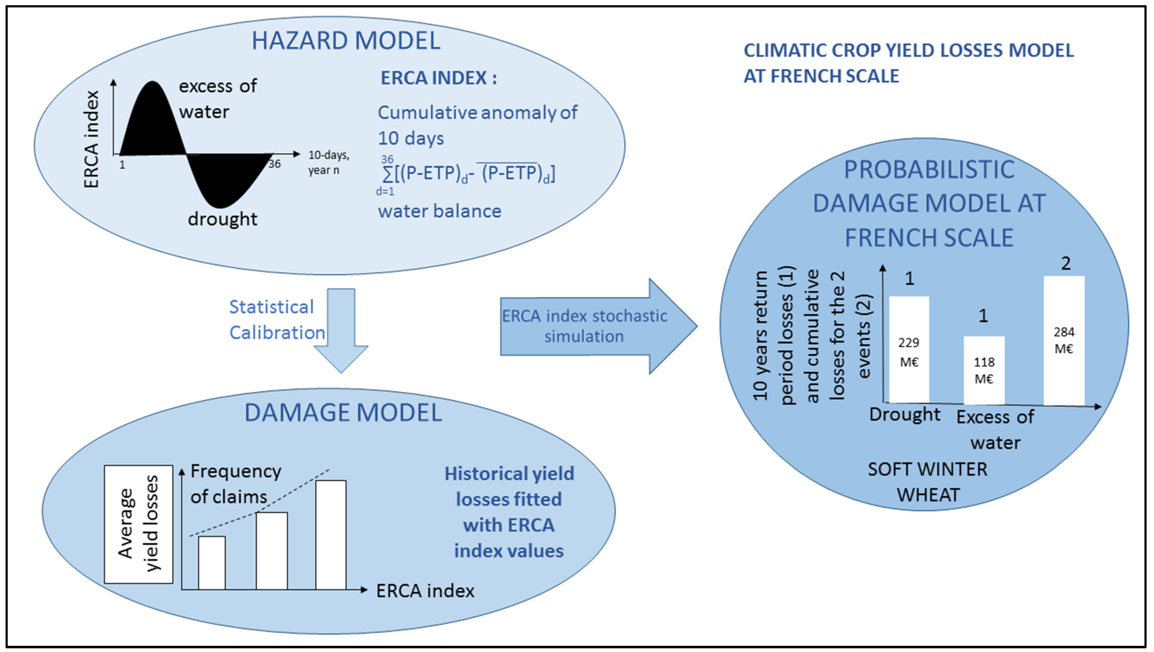
This paper presents the first step of the thesis project: the development of a new index to qualify drought and excess of water and their relationship with yield anomalies (Figure 1). We consider in this paper that both drought and excess of water can be explained by an accumulated simplified soil water balance anomaly based only on precipitation and evapotranspiration balance in the soil–plant system. The choice of the department scale was driven by the availability of yield data. The DOWKI was initially based on the SPEI, computed as a difference between precipitation and evapotranspiration with a different standardization method. Based on the DOWKIdrought and DOWKIwetness, the simulation of extreme yield losses was carried out, along with a prediction of the impact of climate change on crops.
2.1. Input Data
2.1.1. Meteorological Data
The meteorological data used in this paper were measured on a sample of the METEO-FRANCE synoptic network of rain gauges (79 stations). These precipitation and evapotranspiration data have been available since 1989 from these stations. The rainfall data were 10-days cumulative values, measured automatically. The evapotranspiration was estimated by METEO-FRANCE using the Penman equation on a 10-day time scale. For the departments with several stations available, the average of the meteorological parameters was computed.
This restricted choice of stations was voluntarily used to define a global index at the department scale. The data that the index aimed to predict (yield anomalies) were only single annual values.
The study period chosen here to compute the climatic index was 1989–2017. This was related to the availability of crop yield data.
2.1.2. Yield Data and Yield Anomaly Computing
Yield data for several crops (soft winter wheat, winter barley, sunflower) were extracted from the French Ministry of Agriculture (AGRESTE: http://agreste.agriculture.gouv.fr/) database at the department scale. The data were available for the period 1989–2017 (29 years) for winter soft wheat, winter barley, and sunflower. There was no information on irrigated and non-irrigated crops, therefore the yield data included both.
The yield data available consisted of a single value for each year, the actual yield value of the last crop produced and declared on a given surface.
Yield anomalies for the n-th year were computed by comparing the annual yield with a yield reference defined by the Olympic average over five years. This methodology has been used in public policies like the crop insurance developed in the CAP since 2014 [52].
2.2. Computing the DOWKI Index
The index proposed in this paper is called “Drought and Overwhelmed Water Key Indicator” (i.e., DOWKI) and is based on the cumulated difference between efficient rain and 28-year normal efficient rain value at a 10-day time scale within the vulnerability period of the crop.
As a climatic index, it does not require calibration, and its unique parameter is the period of vulnerability of the crop. It is easy to compute with a few input data and has been defined as a single value for each year to be in line with the yield data it has to predict.
The value of the water balance was computed by the following equation:
in which Pi and PETi are the precipitation and potential evapotranspiration of the i-th decade of the year n (values of i were from 1 to 36) and ERi,n is the initial water balance of the i-th decade of the year n. Equation (1) is calculated for the whole year. This “climatic water balance” was adapted from the SPEI index [39]. The difference between these two parameters provides a reliable measure of drought severity not considered only by the parameter P. This makes it possible to qualify different types of drought, especially drought defined by extreme temperatures (i.e., 2003 in France).
Equation (2) was used to standardize the index by calculating the anomaly:
in which is the average of the ERI for each decade i over the entire available history. Then, the values of ERNi,n were added up to create a cumulative index for each decade (36 values in a year) using the following equation:
in which the initial value ERN0,n of the n-th year is equal to zero.
As a pure climatic index, DOWKI does not take into account the soil and crop properties. The component of the hazard is expressed in Equation (3). As a cumulative value calculated over the whole year, this index has no concept of the vulnerability period of the crops, the risk being represented as the crossing of the hazard by the vulnerability of the crop studied. Furthermore, it has been proven that the climatic indicators have the best results when they are computed on the growing season [11]. To integrate this factor, we selected the ERNCi,n values within the vulnerability period of a given crop (4).
As a cumulative anomaly of efficient rain, the DOWKI index is able to simulate drought situations (extreme low values) and excess of water situation (extreme high values). The DOWKI index integrates this parameter and is thus calculated by the following equation:
in which i and j are, respectively, the first and the latest decade of the vulnerability period for the crop c and the year n.
At the end of this computing sequence, two indices were available for each year, station and crop: DOWKIdrought and DOWKIwetness.
2.3. Statistical Analysis/Experimental Design
The climatic index parameters were optimized using an experimental design, which consisted of computing a high number of simulations by varying the parameters: the vulnerability period of a given crop and both drought and excess of water thresholds of the DOWKI index for extreme events, the number of departments to consider as the minimum spatial extent for extreme event definition. For each simulation, the model results were compared with historical yield anomalies at the French territory scale.
The experimental design for the six parameters was defined as following:
- The first 10 days of the vulnerability period of the crop: 1 (1–10 January) to 15 (20–30 May);
- The last 10 days of the vulnerability period of the crop: 18 (20–30 June) to 30 (20–30 October);
- Two extreme event definition thresholds (for drought and excess of water) computed as a percentile of the whole DOWKI distribution for all departments and years: 2nd percentile to 30th percentile;
- Two minimum number of departments concerned by extreme DOWKI values (above threshold) for systemic extreme event definition.
The experimental design consisted of 2880 simulations for all six parameter variations. The robustness of the model was characterized by a list of indicators:
- Average error and percentiles;
- Number of drought and excess of water events;
- Maximum number of true positive (TP);
- Maximum value of the ratio TP/false positive (FP);
- Maximum value of the ratio (sum of anomalies of TP/sum of anomalies of false negative (FN));
- Maximum value of the ratio (average anomaly of TP/ average anomaly of FN);
- Frequency of claims;
- Yield anomalies percentile 90 for the higher class of DOWKIwetness and lower class of the DOWKIdrought;
- Yield anomalies average for the higher class of DOWKIwetness and lower class of the DOWKIdrought;
The model was developed in Matlab for windows and the data were CSV files (Coma Separated Values). The total duration of the experimental design was two hours on a standard computer for the 2880 simulations.
2.4. Calibration of the Damage Models
To calibrate a climatic model based on the index, the statistical relationship between index values and yield anomalies at the department scale was studied. Instead of fitting a probabilistic distribution, a classification of the index was proposed, and the damage indicators were calculated for each class. Based on the analysis of the distributions for both indices, the ranges of values were the following: (0 to −300 of cumulated simplified water balance anomaly (mm) for drought and (0 to 250) for excess of water. For each class, the following parameters were calculated:
- Frequency of claim: (number of years with a yield anomaly above the threshold/total number of years);
- Average value of the yield anomalies above the threshold;
- Distribution of yield anomalies characterized by percentile values (10th, 25th, 50th, 75th, 90th).
Both DOWKI indices were used to simulate drought and excess of water. The two perils were simulated independently. The simulation methodology was based on the calibration matrix defined with the optimized parameters selected by the experimental design. The annual value of DOWKI indices for each year and each department was classified in the calibration matrix. A random value of the loss percentile was computed and a random value of the frequency of claim was applied on each DOWKI value with respect of the class parameters.
By applying this bootstrap simulation method, 1000 repetitions of the simulations were done to compute the confidence interval around the average yield loss simulated values. This first step generated two result matrices for both drought and excess of water. The department results were aggregated at the French scale and compared with historical French scale values.
2.5. Stochastic Simulations of Yield Anomalies Based on the DOWKI Indices
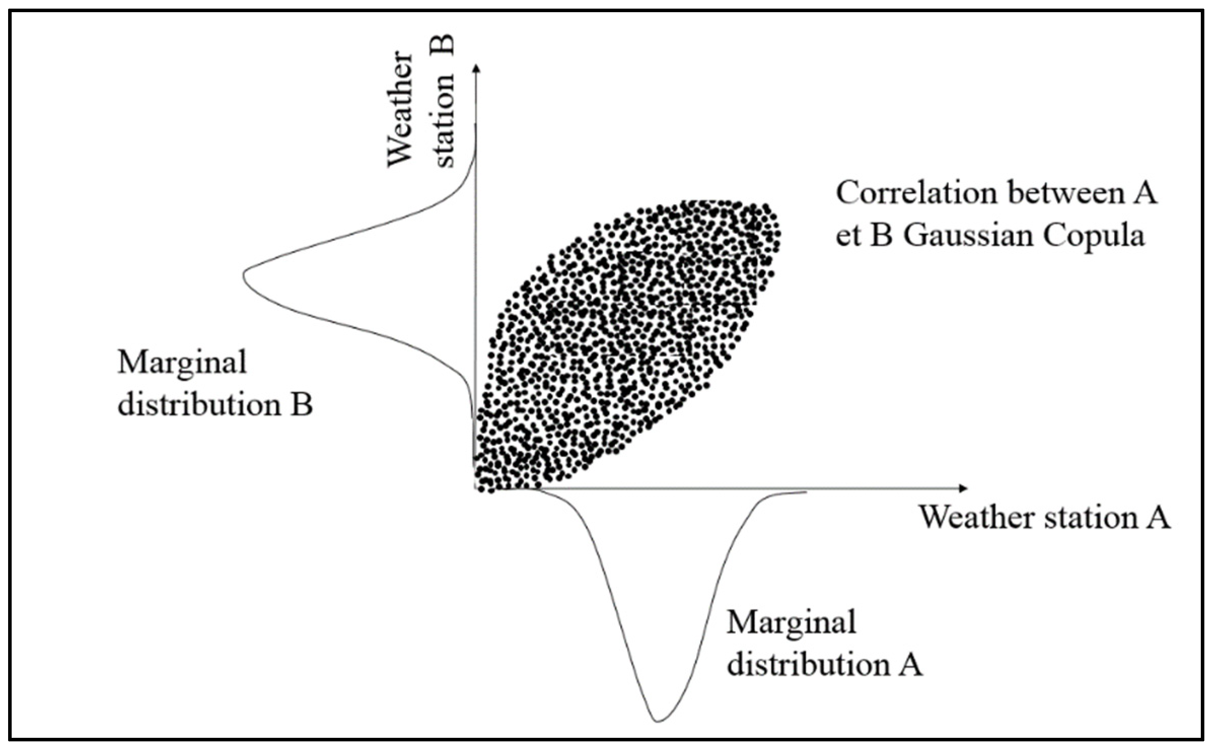
A stochastic model was developed, considering DOWKI values as random values of a predictor. Marginal analysis was conducted at the department scale and spatial correlation was analyzed using a Gaussian copula between departments for the entire historical depth. Gaussian copulas [17,53] were only based on the correlation matrix (Figure 2). No temporal correlation was computed, our hypothesis is that each DOWKI value for year n is independent of the DOWKI value for year n−1. This hypothesis can be discussed, since the soil water content at the end of winter will certainly constrain the DOWKI value of the following year.
The marginal distributions are computed using a Normal model with average and standard deviation of the DOWKI indices as parameters, for drought, and using a bootstrap method, as explained above, for excess of water.
One of the limits of these copula families is their decorrelation for extreme values. Thus, the results of the model will be restricted to low return periods. A different approach (use of a climatic model) will be done in partnership with Meteo-France to allow extreme return period analysis, taking into account the spatial and temporal correlations.
3. Results
3.1. Multi-year ERNC Values for a 10-day Time Step
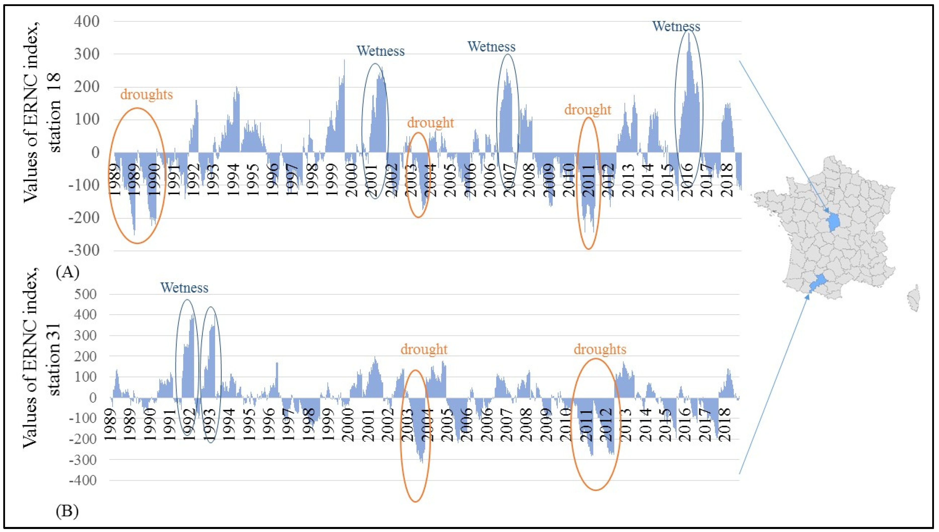
To illustrate the climatic ERNC values, Figure 3 shows the index values per 10-days for stations 18 and 31 for the period 1989–2018.
These stations were chosen to illustrate two different climates in France: station 31 is near Toulouse in the southwestern part of the territory, with an oceanic dry climate and a strong exposure to spring and summer droughts; station 18 is near Bourges in the center of France, with a more continental climate, particularly concerned by the 2016 excess of water event.
The negative values show the dry decades of the historical record, and the positive values the excess of water decades. The most severe droughts clearly appeared on these figures from these years: 1989, 1990, 2003, 2005, 2011, and 2012 (for station 31 only). As seen in Figure 3, excess of water is more of a local event and does not affect all of France in the same years: 2016 was an extreme event in the North of France, 2007 did not affect all of France either. Figure 3 illustrates the dynamics of the index that captured the deficit or excess of water for each decade of the year.
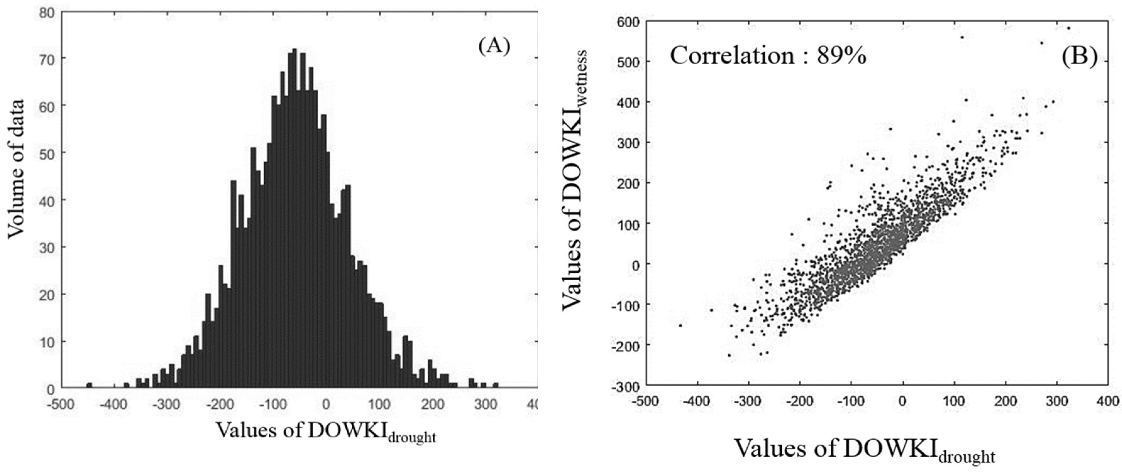
The distribution of DOWKIdrought followed a normal distribution, as shown in Figure 4. Standard values around 0 are non-extreme values with the two following parameters: mean (–66.8) and standard deviation (134.8). The results of the KS (Kolmogorov-Smirnov) test used as a normal distribution test after normalization of the variables (using mean value and standard deviation) with a 5% error were positive. The DOWKIwetness index did not follow exactly a normal distribution (rejected the KS test with 5% error). Thus, to simulate stochastic values of the excess of water index, a bootstrap method was applied, which followed the empirical distribution without the constraint of a probabilistic distribution.
The historical distributions of the two annual indices for drought and excess of water at the department scale were studied in terms of correlation. The correlation coefficient was strong between the two perils (0.89). As shown in Figure 4, this strong positive correlation can be explained: the index for drought was the minimum value of the accumulated water balance during the vulnerability period of the year, whereas the excess of water index was the maximum value.
For extreme drought events in a department, the water balance anomaly never recovered to a normal value. In this case, the excess of water value remained low. On the contrary, the drought index remained high when an extreme excess of water event occurred. Both perils never occurred in the same department during the same year on the historical dataset.
Based on these conclusions, the simulation of one index will force the simulation of the second index to consider the dependence of both perils.
The DOWKI indicators were defined to simulate yield anomalies and extreme event losses, i.e., drought and excess of water events that concern a large geographical extent and elevated losses (represented by yield anomalies) for agriculture at the department level.
Two parameters were selected to constitute the event sets:
- The number of departments concerned by extreme values of DOWKI index;
- The threshold defining extreme values of DOWKI index (a quantile on the global DOWKI distribution for France for the historical period).
The event set was constituted by yearly events for each peril: defined with the annual values of the DOWKI index for each department and to predict annual yield anomalies.
The difficulty in defining the values of the two parameters for extreme event definition was turned around by integrating the parameter selection in the experimental design for model fine tuning.
3.2. Calibration of the Damage Models
The main objective of this paper was to use the DOWKI index to predict yield anomalies for extreme climatic events at the departmental scale. For this purpose, three calibration matrices were built at the department scale, combining hazard values and historical yield anomalies:
- One for drought events (defined by the index threshold and the number of departments concerned);
- One for excess of water events;
- One for the attritional years (no drought and no excess of water).
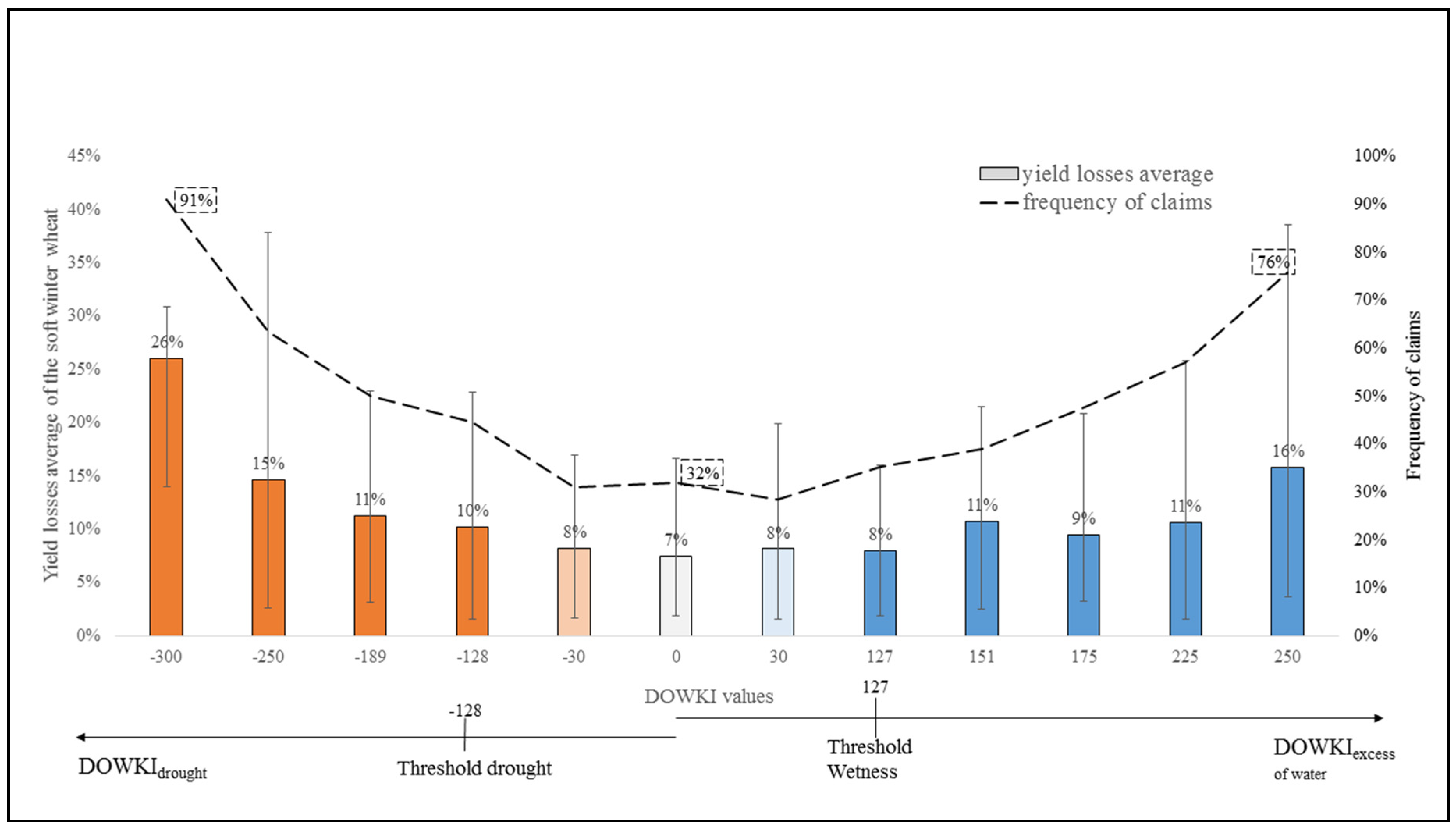
The distribution of yield anomalies within each class and the average value of the claim frequency is described in Figure 5 for winter soft wheat. This figure illustrates the DOWKI capacity to predict the occurrence of a yield anomaly and the intensity of the loss. Indeed, a high frequency of claims were calculated for the extreme values of the DOWKI (for drought and wetness)—probability of 91% to observe a claim when the DOWKI value is below −300 and probability of 76% when the DOWKI value is above 250.
On the contrary, when DOWKI values were close to zero, the probability of claims was significantly lower (~30%). We postulate that values of DOWKI below the drought and excess of water thresholds represent natural fluctuations around the Olympic average, which is consistent with the observed low frequency of claims.
The average and min/max values of yield anomalies were significantly higher when the DOWKI value exceeded the threshold. Nevertheless, for every DOWKI class, a substantial number of departments did not show yield anomalies. Many hypotheses can be formulated to explain these false positives:
- A parameter was not included in the DOWKI calculation (e.g., temperature, soil water content);
- Adaptation of the agricultural practices (modifying the sowing period and harvest period, choice of varieties);
- Protection measures: the irrigation information was not provided in the AGRESTE database and can significantly change yield anomalies in case of extreme drought.
Investigations were carried out on the class values to explain the fluctuations of yield anomalies for a given DOWKI class. High yield anomalies for low DOWKI values could be explained by the occurrence of non-modeled hazard: a frost event in 2003, responsible for high losses during a year also characterized by an extreme drought. The major difficulty in the yield anomaly analysis was the multi-causal effect: abnormal yield values can be due to a combination of hazard and anthropic choices that are not described in the AGRESTE data. For this reason, the DOWKI index is calibrated to optimize the damage model only for extreme events, during which the other causes are considered as insignificant.
The selected model parameters for the Figure 5 computation were the following: 12th decade (3rd decade of April) 22nd decade (1st decade of August), quantiles 20th for drought and 80th for excess of water. Minimum number of departments: 20 for drought and 35 for excess of water. The analysis of the simulation on the historical event set showed:
- An average yield prediction error (and error quantiles 10:25:75:90): 0.039 (−0.33:−0.11:0.25:0.34) for drought;
- For excess of water: 0.077 (−0.35:−0.14:0.29:0.33).
This calibration matrix was input data for the damage model. The calibration values were strongly dependent on the model parameters. To assess the impact of parameter variations, an experimental design was conducted.
3.3. Experimental Design Results and Parameters Sensitivity
The experimental design aimed to calibrate the model n times (n representing the number of combinations of all chosen parameter values) on the historical DOWKI values and yield losses. The n calibration matrices were saved in a global file and applied to the historical DOWKI values calculated for drought and excess of water at the department scale. The number of historical events simulated depended on the extreme event definition: number of departments concerned and DOWKI extreme threshold value. For each event, the average, 10th and 90th percentile simulated value of the loss ratios for yield anomalies were calculated and compared with the historical values. This made it possible to calculate the uncertainties for each event, depending on the whole model and extreme event definition parameters.
For the 2880 simulations of the experimental design, the average error of the model was 17% for drought and 5.3% for excess of water. The 10th and 90th percentile interval of the error distribution were respectively −12% and −49%, and −27% and −20%. Among the six parameters of the experimental design, the effect of their variations was quantified for prioritization.
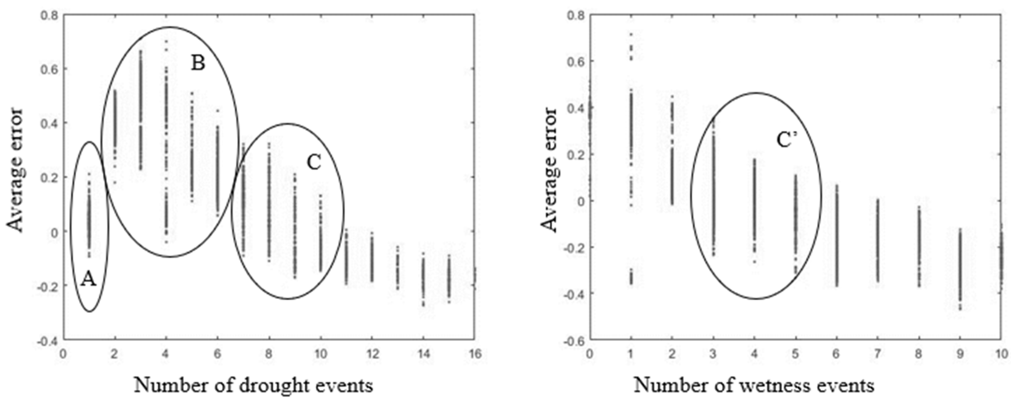
The results of the experimental design indicate that the number of events taken into account for model calibration had the most impact on the average error distribution (Figure 6). The number of events depended on two parameters: number of departments and thresholds of the DOWKI indices.
As shown in Figure 6, the average error was minimized for a number of droughts between eight and ten (C), and between three and five (C’) for excess of water events. Note that Figure 6 describes soft winter wheat and specific experimental designs were simulated for winter barley, maize, and sunflower for the best parameter selection.
The elevated uncertainties of the yield anomaly predictions can be due to external factors (natural hazard, geographical location within the department, diseases) or internal factors (agricultural decisions, prevention measures). To improve the internal factor uncertainties, a downscaling of the model at the farm scale will be done in the next steps of the project.
The calibration of DOWKI versus yield losses was easier for drought than for excess of water. One explanation is the number of drought events is more important and makes it possible to use more data for calibration. The excess of water can also be more difficult to characterize due to indirect damages: impossibility of the farmers having access to the drenched agricultural fields or river flood.
At the end of the experimental design, a deterministic model was developed with measured uncertainties to predict the agricultural crop yields from the calculation of the DOWKI index at the station/department scale. The model was validated for drought and excess of water for the extreme events, defined as systemic events. This model can be used to evaluate the yield losses at the end of the agricultural season, as soon as precipitation and evapotranspiration data are available. This model can also be used for pricing the insurance contracts on the historical data. Nevertheless, the exposure measure was not complete, with only 30 years of recording, since the extreme events frequency is very low by definition. Thus, a stochastic version of the model has been developed to take into account a large number of extreme events.
3.4. Stochastic Simulations and Extreme Value Analysis
The next step was to simulate a large number of years of DOWKI values, taking into account the spatial and temporal correlation of the indices in order to apply the damage model. The expected result of the model is the frequency/intensity distribution of yield losses, the basis of the pricing models of insurance, and the capacity to predict the loss values for different return periods. The stochastic distributions were then compared with the historical distribution to perform the model validation.
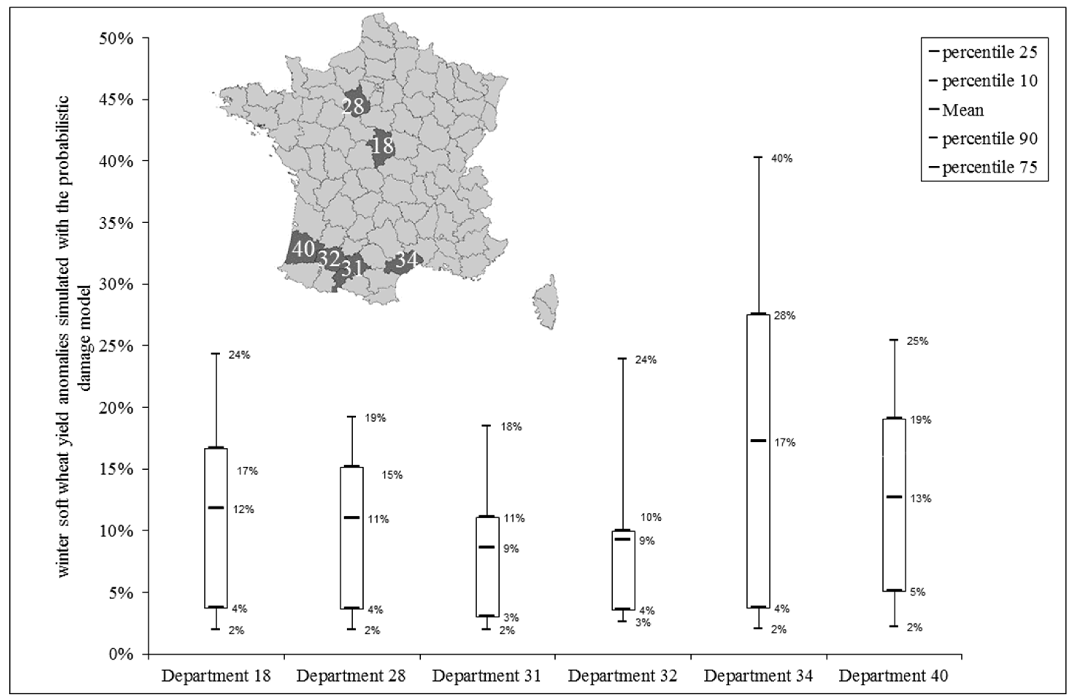
Figure 7 illustrates the distribution of 5000 years of yield anomalies simulated with the stochastic drought model for several departments. Departments 18 and 28 are located in the center of France, departments 31 and 32 are located in the southwest, and departments 34 and 40 are located near the sea (respectively, the Mediterranean Sea and Atlantic Ocean). For each distribution the percentage of null values (years with no extreme drought event or above average yield) was calculated: departments 18 and 28 (85.7% and 88.7%), departments 31 and 32 (86.6% and 87.2%), departments 34 and 40 (89.6% and 86.0%). These results show the homogeneity of the yield anomalies simulated for comparable climate departments. The occurrence of drought events was rare for department 34 but the yield anomalies were expected to be higher when an event occurs. On the contrary, departments 31 and 32 showed similar results, with slightly higher risk of drought but lower yield anomalies when it occurs. This can also be explained by the more important soft wheat production in these departments, averaging the loss values between different locations. Departments 18 and 28 showed comparable yield anomalies, but with a higher exposure to drought events for department 18. Department 40 had an extreme event probability of occurrence similar to departments 18 and 31 but with higher yield losses. Here again, the lower soft wheat production in this region can explain the higher volatility of the results.
These results illustrate the use of the stochastic model for drought and its capacity to simulate the exposure to yield anomalies. The same analysis was done for excess of water events but is not represented here.
These results can be used for insurance premium pricing at the field or farm level, the average yield loss value can be considered the premium ratio applied to the capital value at risk. The standard deviation or the quantiles of the yield loss ratio are usually integrated into premium calculation by the insurers to take into account the loss volatility. These first results of the model present at this state an application in the insurance field and the highest variability of the yield losses for some departments (34, and to a lesser extent 18 and 40) illustrates the higher exposure of soft wheat on these regions.
The next step of the insured loss exposure simulation was to apply the loss ratio to the insured values of the crops at the department scale. To estimate these insured values, the average yield production at the department scale was multiplied by department crop production surface and the insured price index given by the multirisk crop insurance technical report [52]. The price index for soft winter wheat was 176 €/T, for sunflower 485 €/T, and winter barley 178 €/T. We compared the model results with the historical losses calculated using the same methodology applied on the historical yield loss ratios (Table 1).
The results given here provide information about the potential insured risk if all the French farms were covered by insurance contracts. This important theorical value represents the simulated maximum claim for a whole France portfolio. This type of study could bring elements for discussion in the insurance crop reform. The use of price index values for insured value estimations allowed us to avoid the difficulty of price modeling and the impact of the price variation on the economic losses.
These loss ratios were calculated for the whole French farm for each crop and could be used to assess the financial losses. For example, for 5 million hectares of winter soft wheat, an average yield of 80 q/ha, the average, 10 year, and 100 year losses due to drought were estimated to be M€54.2, M€229.0, and M€690.1. Furthermore, a theorical pure premium for insurance could be estimated, taking into account the uncertainties, to 1.09% of production value for soft wheat for drought and 0.54% for soft wheat for excess of water.
4. Discussion
The DOWKI index was developed to simulate extreme drought and excess of water events and their impact on yield losses at the department scale. The DOWKI index has a pure meteorological basis (10 day time-step rainfall and evapotranspiration). The capacity of the soil reservoir and soil porosity are not taken into account in this model. Indeed, at the department scale, the variability in the soil composition would make it difficult to synthesize in a global characterization. The meteorological conditions can be considered more homogeneous. This index is easy to figure out and was evaluated with the historical yield losses.
Nevertheless, the use of the ARPEGE-Climat 8 × 8 km grid will probably make it possible to use a spatial method and calculate the DOWKI index on a grid. Then, combining the DOWKI index with a soil map will be practicable. Based on the current calculation of the DOWKI index, one of the limits is the location of agricultural parcels in relation to the Meteorological stations. Indeed, the extrapolation to the department seems difficult, as it may have significantly different climates: for example, plains and mountains in the same department leads to very different weather conditions. The use of GIS (Geographic Information System) to add the different layers of meteorological station location with the parcel register map would be of great use. However, this difficulty will be removed when switching to the 8 × 8 grid with the ARPEGE-Climat model of Meteo-France. The DOWKI index will be calculated for each grid and then the grid value added to the Parcel Register Map for each crop to compute a functional average value of the index at the department scale.
Based on the hypothesis that a physical hazard model does not need complex calibration if the input data are carefully selected, our DOWKI index is easy to calculate on a 10-day meteorological dataset and does not require calibration. The parameters of the model are only designed for the vulnerability part: beginning and end of the vulnerability period of a given crop and minimum geographical extend of the “extreme event” definition.
Our entire calibration and validation method was based on the definition of extreme events for drought and excess of water. Indeed, the (re)insurance industry is concerned by the climatic accident and the prevention measures that can be taken to mitigate their catastrophic effects. The long-term trends of yields in the future will not have an impact on the insurance premium and exposure, as it remains a major issue for the future of agriculture and economy of our countries.
The index has been proven to fit with extreme yield anomalies at the department scale. For the extreme values of our index, both for drought and excess of water, more than 80% of the crops suffered losses with destruction rates (averaged at the department scale) that can reach an average value of 25%. The distribution of farm scale anomaly within a department will present more variability around this average value and will be studied in the former part of this project research.
Yet, yield anomalies on field crops can not only be explained by these two perils alone. Many other factors must be considered to simulate the reality of yield variations around a given threshold. Some of these factors were described in this paper:
- Human decisions: irrigation, sowing dates, alternative crops, cultivation methods and options, all preventive measures taken by the farmer with the objective to reduce the impact of the climatic events during the season;
- Non meteorological natural factors: soil nature, micro-relief (slopes, depressions, exposition);
- Not modeled climatic perils: frost, hail.
Our model only aimed to explain the yield anomalies due to extreme climatic events occurring during the growing period of the crop. In this case, we postulate that other factors are negligible.
Nevertheless, our modeling method underestimated yield anomalies occurring during the seasons without any extreme climatic event. The average yield anomalies computed on the past or for the stochastic event set distribution were potentially underestimated.
Our pure climatic index reflects the potential claims due to extreme drought and excess of water events but the reality of the yield variations includes human decisions. Our main objective was to use our model for climatic projections at the horizon 2050, by linking the DOWKI model with the Meteo-France ARPEGE-Climat modeling. Our model will have to be completed with hypotheses regarding the vulnerability of farms and human decisions.
Nevertheless, the (re)insurance industry and public institutions are facing a lack of data on the climatic evolution of extreme losses under a climate change paradigm. Our climatic projections, based on the DOWKI index, will provide trends for yield losses, all other things remaining equal. Of course, the authors are aware that production systems will evaluate to mitigate the impact of climate change. However, 2050 is a short-term perspective (~30 years from now) and the inertia of the production systems must be taken into account. Our simulations under current climate conditions have been validated by comparison with the historical losses in this paper. Thus, future projections will rely on a solid basis.
For example, we computed M€82.0 annual losses for soft winter wheat, compared with M€1114 at the French farm scale. The difference between those two values can be explained by not modeled factors and small yield variations. Yet, the simulated SMP (potential maximum claim) was M€1403.2, compared with the historical M€846.0. The extreme losses for drought and excess of water simulated were significantly higher than the higher historical loss.
The knowledge of extreme claims under current climate conditions will provide further input to advocate stronger public policies for risk management, at the national and European scale. The development of insurance products and the sustainability under a climate change context remain a fundamental point for in-depth discussions about risk management tools.
5. Conclusions
A new climatic index was proposed in this paper in order to predict crop yield anomalies due to drought and excess of water. The calibration and validation of this index has made it possible to run stochastic simulations of yield anomalies within the current climate conditions. An evaluation of the financial exposure of the French farm has been performed, with numerous uncertainties at this step of the model development.
The global objective of this multi-year project is to predict the impact of climate change on the financial exposure of (re)insurance companies. For this purpose, the focus was on extreme events, which concern a large part of the French territory and will have an impact on a global insurance portfolio.
The next steps of the project, in partnership with Meteo-France, will be to apply our model on the ARPEGE-Climat simulations to predict evolution of the yield losses due to climate change for the 2050 horizon [19,54,55]. For this future study, two sets of climatic simulations will be available for this project: 400 simulations of the same year in current climate conditions (year 2000) and 400 simulations in future climate conditions, with the RCP 8.5 (Representative Concentration Pathway) forcing values (year 2050). Precipitation and evapotranspiration data will be available on the SAFRAN 8 × 8 km grid and the DOWKI model will be applied to predict yield anomalies in current and future climate conditions.
Author Contributions
Validation, J.C.; Writing—original draft, D.K. and D.M.
Funding
This research received no external funding.
Acknowledgments
The authors want to thank Martine Veysseire from Météo-France for the production of ARPEGE-Climat simulations.
Conflicts of Interest
The authors declare no conflict of interest.
References
- IPCC. Managing the Risks of Extreme Events and Disasters to Advance Climate Change Adaptation; Cambridge University Press: Cambridge, UK; New York, NY, USA, 2012; p. 582. [Google Scholar]
- Van der Velde, M.; Tubiello, F.N.; Vrieling, A.; Bouraoui, F. Impacts of extreme weather on wheat and maize in France: Evaluating regional crop simulations against observed data. Clim. Chang. 2012, 113, 751–765. [Google Scholar] [CrossRef]
- Ciais, P.; Reichstein, M.; Viovy, N.; Granier, A.; Ogée, J.; Allard, V.; Aubinet, M.; Buchmann, N.; Bernhofer, C.; Carrara, A.; et al. Europe-wide reduction in primary productivity caused by the heat and drought in 2003. Nature 2005, 437, 529–533. [Google Scholar] [CrossRef] [PubMed]
- COPA-COGECA. Assessment of the Impact of the Heat Wave and Drought of the Summer 2003 on Agriculture and Forestry; Committee of Agricultural Organisations in the European Union and General Committee for Agricultural cooperation in the European Union: Brussels, Belgium, 2003; pp. 1–15. [Google Scholar]
- Bazzaz, F.; Sombroek, W. Changements du Climat et Production Agricole; FAO: Rome, Italy, 1997; ISBN 92-5-203987-2. [Google Scholar]
- Lobell, D.B.; Schlenker, W.; Costa-Roberts, J. Climate Trends and Global Crop Production Since 1980. Science 2011, 333, 616–620. [Google Scholar] [CrossRef] [PubMed] [Green Version]
- Olesen, J.E.; Trnka, M.; Kersebaum, K.C.; Skjelvag, A.O.; Seguin, B.; Peltonen-Sainio, P.; Rossi, F.; Kozyra, J.; Micale, F. Impacts and adaptation of European crop production systems to climate change. Eur. J. Agron. 2011, 34, 96–112. [Google Scholar] [CrossRef]
- Challinor, A.J.; Watson, J.; Lobell, D.B.; Howden, S.M.; Smith, D.R.; Chhetri, N. A meta-analysis of crop yield under climate change and adaptation. Nat. Clim. Chang. 2014, 4, 287–291. [Google Scholar] [CrossRef]
- Gouache, D.; Bouchon, A.-S.; Jouanneau, E.; Le Bris, X. Agrometeorological analysis and prection of wheat yield at the departmental level in France. Agric. For. Meteorol. 2015, 209–210, 1–10. [Google Scholar] [CrossRef]
- Mathieu, J.A.; Aires, F. Assessment of the agro-climatic indices to improve crop yield forecasting. Agric. For. Meteorol. 2018, 253–254, 15–30. [Google Scholar] [CrossRef]
- Ben-Ari, T.; Adrian, J.; Klein, T.; Calanca, P.; Van der Velde, M.; Makowski, D. Identifying indicators of extreme wheat and maize yield losses. Agric. For. Meteorol. 2016, 220, 130–140. [Google Scholar] [CrossRef]
- Schlenker, W.; Roberts, M.J. Nonlinear temperature effects indicate severe damages to U.S. crop yields under climate change. Proc. Natl. Acad. Sci. USA 2009, 106, 15594–15598. [Google Scholar] [CrossRef] [Green Version]
- Amigues, J.P.; Debaeke, P.; Itier, B.; Lemaire, G.; Seguin, B.; Tardieu, F.; Thomas, A. Sécheresse et Agriculture. Réduire la Vulnérabilité de L’agriculture à un Risque Accru du Manque D’eau; INRA: Paris, France, 2006; p. 72. [Google Scholar]
- Bourcier, V.; Carrega, M.; Corona, C.; Degache-Masperi, A.; Duvernoy, J.; Eckert, N.; Etchevers, P.; Faug, T.; Habets, F.; Giacona, F.; et al. Les Événements Météorologiques Extrêmes Dans un Contexte de Changement Climatique; La documentation Française; ONERC: Paris, France, 2019; p. 200. [Google Scholar]
- IPCC. Climate Change 2007: Impacts, Adaptation and Vulnerability. Contribution of Working Group II to the Fourth Assessment Report of the Intergovernmental Panel on Climate Change; Cambridge University Press: Cambridge, UK; New York, NY, USA, 2007; p. 976. [Google Scholar]
- COM. Proposal for a Regulation of the European Parliament and of the Council Establishing Rules on Support Ofr Strategic Plans to Be Drawn up by Member States under the Common Agricultural Policy (CAP Strategic Plans) and Financed by the European Agricultural Guarantee Fund (EAGF) and by the European Agricultural Fund for Rural Development (EAFRD) and Repealing Regulation (EU) No 1305/2013 of the European Parliament and of the Council and Regulation (EU) No 1307/2013 of the European Parliament and of the Council. 2018. Available online: https://eur-lex.europa.eu/legal-content/EN/TXT/?uri=COM%3A2018%3A392%3AFIN (accessed on 24 October 2019).
- Moncoulon, D.; Labat, D.; Ardon, J.; Leblois, E.; Onfroy, T.; Poulard, C.; Aji, S.; Rémy, A.; Quantin, A. Analysis of the French insurance market exposure to floods: A stochastic model combining river overflow and surface runoff. Nat. Hazards Earth Syst. Sci. 2013, 1, 3217–3261. [Google Scholar] [CrossRef]
- Naulin, J.P.; Moncoulon, D.; Le Roy, S.; Pedreros, R.; Idier, D.; Oliveros, C. Estimation of insurance-related losses resulting from coastal flooding in France. Nat. Hazards Earth Syst. Sci. 2016, 16, 195–207. [Google Scholar] [CrossRef]
- Moncoulon, D.; Veysseire, M.; Naulin, J.-P.; Wang, Z.-X.; Tinard, P.; Desarthe, J.; Hajji, C.; Onfroy, T.; Regimbeau, F.; Déqué, M. Modelling the evolution of the financial impacts of flood and storm surge between 2015 and 2050 in France. Int. J. Saf. Secur. Eng. 2016, 6, 141–149. [Google Scholar] [CrossRef] [Green Version]
- Kapsambelis, D.; Moncoulon, D.; Veysseire, M.; Cordier, J. Impact of Climate Change on Agricultural Economic Losses in France: Modelling Drought and Frost Events in 2050 and Their Impact on Agricultural Yield Loss Rates; European Meteorological Society, Berlin: Lyngby, Denmark, 2019; Volume 16, p. 130. [Google Scholar]
- OMM; GWP. Programme de Gestion Intégrée des Sécheresses. In Manuel des Indicateurs et Indices de Sécheresse; Svoboda, M., Fuchs, B.A., Eds.; OMM: Genève, Switzerland, 2016. [Google Scholar]
- Banimahd, S.A.; Khalili, D. Factors Influencing Markov Chains Predictability Characteristics, Utilizing SPI, RDI, EDI, and SPEI Drought Indices in Different Climatic Zones. Water Resour. Manag. 2013, 27, 3911–3928. [Google Scholar] [CrossRef]
- Palmer, W.C. Meteorological Droughts; Weather Bureau Research Paper; U.S. Department of Commerce: Washington, DC, USA, 1965; p. 58.
- Karl, T.R. Some spatial characteristics of drought duration in the United States. J. Clim. Appl. Meteorol. 1983, 22, 1356–1366. [Google Scholar] [CrossRef]
- Karl, T.R. The sensitivity of the Palmer Drought Severity Index and Palmer’s Z-Index to their calibration coefficients including Potential Evapotranspiration. J. Clim. Appl. Meteorol. 1986, 25, 77–86. [Google Scholar] [CrossRef]
- Alley, W.M. The Palmer Drought Severity Index: Limitationd and assumptions. J. Clim. Appl. Meteorol. 1984, 23, 1100–1109. [Google Scholar] [CrossRef]
- Guttman, N.B. Comparing the palmer drought index and the standardized precipitation index1. J. Am. Water Resour. Assoc. 1998, 34, 113–121. [Google Scholar] [CrossRef]
- Wells, N.; Goddard, S.; Hayes, M.J. A self-Calibrating Palmer Drought Severity Index. J. Clim. 2004, 17, 2335–2351. [Google Scholar] [CrossRef]
- McKee, T.B.; Doesken, N.J.; Kleist, J. The Relationship of Drought Frequency and Duration to Time Scales. In Proceedings of the Eighth Conference on Applied Climatology; American Meteorological Society: Boston, MA, USA, 1993; pp. 179–184. [Google Scholar]
- Byun, H.R.; Wilhite, D.A. Daily quantification of drought severity and duration. J. Clim. 1996, 5, 1181–1201. [Google Scholar]
- Lobell, D.B.; Hammer, G.L.; McLean, G.; Messina, C.; Roberts, M.J.; Schlenker, W. The critical role of extreme heat for maize production in the United States. Nat. Clim. Chang. Lett. 2013, 3, 497–501. [Google Scholar] [CrossRef]
- Iizumi, T.; Ramankutty, N. Changes in yield variability of major crops for 1981–2010 explained by climate change. Environ. Res. Lett. 2016, 11, 34003. [Google Scholar] [CrossRef]
- Teixeira, E.I.; Fischer, G.; van Velthuizen, H.; Walter, C.; Ewert, F. Global hot-spots of heat stress on agricultural crops due to climate change. Agric. For. Meteorol. 2013, 170, 206–215. [Google Scholar] [CrossRef]
- Ray, D.K.; Gerber, J.S.; MacDonald, G.K.; West, P.C. Climate variation explains a third of global crop yield variability. Nat. Commun. 2015, 6, 5989. [Google Scholar] [CrossRef] [PubMed]
- Beguería, S.; Vicente-Serrano, S.M.; Reig, F.; Latorre, B. Standardized precipitation evapotranspiration index (SPEI) revisited: Parameter fitting, evapotranspiration models, tools, datasets and drought monitoring. Int. J. Climatol. 2014, 34, 3001–3023. [Google Scholar] [CrossRef]
- Ayanlade, A.; Radeny, M.; Morton, J.F.; Muchaba, T. Rainfall variability and drought characteristics in two agro-climatic zones: An assessment of climate change challenges in Africa. Sci. Total Environ. 2018, 630, 728–737. [Google Scholar] [CrossRef]
- Rebetez, M.; Mayer, H.; Dupont, O.; Schindler, D.; Gartner, K.; Kropp, J.P.; Menzel, A. Heat and drought 2003 in Europe: A climate synthetis. Ann. For. Sci. 2006, 63, 569–577. [Google Scholar] [CrossRef]
- Potop, V.; Možný, M.; Soukup, J. Drought evolution at various time scales in the lowland regions and their impact on vegetable crops in the Czech Republic. Agric. For. Meteorol. 2012, 156, 121–133. [Google Scholar] [CrossRef]
- Vicente-Serrano, S.M.; Beguería, S.; López-Moreno, J.I. A multiscalar drought index sensitive to global warming: The Standardized Precipitation Evapotranspiration Index. J. Clim. 2010, 23, 1696–1718. [Google Scholar] [CrossRef]
- Donohue, R.; McVicar, T.; Roderick, M. Assessing the ability of potential evaporation formulations to capture the dynamics in evaporative demand within a changing climate. J. Hydrol. 2010, 386, 186–197. [Google Scholar] [CrossRef]
- Tsakiris, G.; Vangelis, H. Establishing a Drought Index Incorporating Evapotranspiration. Eur. Water 2005, 9/10, 3–11. [Google Scholar]
- Woli, P.; Jones, J.W.; Ingram, K.T.; Fraisse, C.W. Agricultural reference index for drought (ARID). Agron. J. 2012, 104, 287–300. [Google Scholar] [CrossRef]
- Fu, B.P. On the calculation of the evaporation from and surface. Chin. J. Atmos. Sci. 1981, 5, 23–31. (In Chinese) [Google Scholar]
- Pagani, V.; Guarneri, T.; Fumagalli, D.; Movedi, E.; Testi, L.; Klein, T.; Calanca, P.; Villalobos, F.; Lopez-Bernal, A.; Niemeyer, S.; et al. Improving cereal yield forecasts in Europe—The impact of weather extremes. Eur. J. Agron. 2017, 89, 97–106. [Google Scholar] [CrossRef]
- Sepulcre-Canto, G.; Horion, S.; Singleton, A.; Carrao, H.; Vogt, J. Development of a Combined Drought Indicator to detect agricultural drought in Europe. Nat. Hazards Earth Syst. Sci. 2012, 12, 3519–3531. [Google Scholar] [CrossRef] [Green Version]
- Anderson, M.C.; Hain, C.; Wardlow, B.; Pimstein, A.; Mecikalski, J.R.; Kustas, W.P. Evaluation of drought indices based on hermal Remote Sensing of evapotranspiration over the continental United States. J. Clim. 2011, 24, 2025–2044. [Google Scholar] [CrossRef]
- Huete, A.R.; Didan, K.; Miura, T.; Rodriguez, E.P.; Gao, X.; Ferreira, L.G. Overview of the radiometric and biophysical performance of the MODIS vegetation indices. Remote Sens. Environ. 2002, 83, 195–213. [Google Scholar] [CrossRef]
- Gao, B.-C. NDWI—A Normalized Difference Water Index for Remote Sensing of vegetation liquid water from space. Remote Sens. Environ. 1996, 58, 257–266. [Google Scholar] [CrossRef]
- Kogan, F.N. Application of vegetation index and brightness temperature for drought detection. Adv. Space Res. 1995, 15, 91–100. [Google Scholar] [CrossRef]
- Brown, J.F.; Wardlow, B.D.; Tadesse, T.; Hayes, M.J.; Reed, B.C. The Vegetation Drought Response Index (VegDRI): A new integrated approach for monitoring drought stress in vegetation. GISci. Remote Sens. 2008, 45, 16–46. [Google Scholar] [CrossRef]
- Roumiguié, A.; Jacquin, A.; Sigel, G.; Hervé, P.; Lepoivre, B.; Hagolle, O. Development of an index-based insurance product: Validation of a forage production index derived from medium spatial resolution fCover time series. GISci. Remote Sens. 2015, 52, 94–113. [Google Scholar] [CrossRef]
- Ministère de l’Agriculture, de l’Agroalimentaire et de la Foret, Ministère de l’Economie et des Finances Cahier des charges applicable aux entreprises d’assurance pour la prise en charge partielle de primes et cotisations d’assurance récolte 2016. Pris en application des articles 1, 2 et 10 du décret fixant pour les années 2016-2020 les modalités d’application de l’article L. 361-4 du code rural et de la pêche maritime en vue de favoriser le développement de l’assurance contre certains risques agricoles. 2016. Available online: https://www.legifrance.gouv.fr/affichTexte.do?cidTexte=JORFTEXT000037330968&categorieLien=id (accessed on 24 October 2019).
- Sklar, A. Fonctions de repartition à n dimensions et leurs marges. Institut Statistique de l’Université de Paris 1959, 8, 229–231. [Google Scholar]
- Moncoulon, D.; Desarthe, J.; Naulin, J.-P.; Onfroy, T.; Tinard, P.; Wang, Z.-X.; Hajji, C.; Veysseire, M.; Dequé, M.; Régimbeau, F. Conséquences du Changement Climatique sur le Coût des Catastrophes Naturelles en France à L’horizon 2050; Caisse Centrale de Réassurance & Météo: Paris, France, 2018; p. 31. [Google Scholar]
- Caisse Centrale de Réassurance. Modélisation de L’impact du Changement Climatique sur les Dommages Assurés Dans le Cadre du Régime Catastrophes Naturelles; Caisse Centrale de Réassurance: Paris, France, 2015. [Google Scholar]
Figure 1.
Schematic representation of the general methodology of the model: from climatic index to stochastic loss modeling.
Figure 1.
Schematic representation of the general methodology of the model: from climatic index to stochastic loss modeling.

Figure 2.
Gaussian copula and empirical distributions of the Drought and Overwhelmed Water Key Indicator (DOWKI) indices for two weather stations.
Figure 2.
Gaussian copula and empirical distributions of the Drought and Overwhelmed Water Key Indicator (DOWKI) indices for two weather stations.

Figure 3.
ERNC indices for stations 18 (A) and 31 (B) for the period 1989–2018. Examples of drought and excess of water events detected from the ERNC chronology. (A) is characterized by a southern oceanic climate with dry summers and (B) by a northern modified oceanic climate.
Figure 3.
ERNC indices for stations 18 (A) and 31 (B) for the period 1989–2018. Examples of drought and excess of water events detected from the ERNC chronology. (A) is characterized by a southern oceanic climate with dry summers and (B) by a northern modified oceanic climate.

Figure 4.
(A) Empirical distribution of the DOWKIdrought values at the department scale calculated on the historical data. (B) Correlation between the indices DOWKIdrought and DOWKIwetness: one data being one year/one department.
Figure 4.
(A) Empirical distribution of the DOWKIdrought values at the department scale calculated on the historical data. (B) Correlation between the indices DOWKIdrought and DOWKIwetness: one data being one year/one department.

Figure 5.
Damage functions for soft winter wheat yield loss simulations: frequency of claims, percentile 10 and 90, average of yield losses according to DOWKI values.
Figure 5.
Damage functions for soft winter wheat yield loss simulations: frequency of claims, percentile 10 and 90, average of yield losses according to DOWKI values.

Figure 6.
Results of experimental plan: average error depending on the number of drought and excess of water events. Three panels identified as examples. A: only one event for calibration; B: between two and six events; C and C’: best distribution of average error.
Figure 6.
Results of experimental plan: average error depending on the number of drought and excess of water events. Three panels identified as examples. A: only one event for calibration; B: between two and six events; C and C’: best distribution of average error.

Figure 7.
Simulated yield anomalies caused by drought for winter soft wheat simulated with the probabilistic model. Department 34 is characterized by a Mediterranean climate, department 31, 32, and 40 by a southern oceanic climate, and department 18 and 28 by a northern modified oceanic climate.
Figure 7.
Simulated yield anomalies caused by drought for winter soft wheat simulated with the probabilistic model. Department 34 is characterized by a Mediterranean climate, department 31, 32, and 40 by a southern oceanic climate, and department 18 and 28 by a northern modified oceanic climate.


Table 1.
Comparison of estimated historical and simulated damages (M€)—average and maximum—at the French farm scale for three field crops: soft winter wheat, winter barley, and sunflower.
Table 1.
Comparison of estimated historical and simulated damages (M€)—average and maximum—at the French farm scale for three field crops: soft winter wheat, winter barley, and sunflower.
| Crop | Simulated Average Annual Losses (10th Percentile–90th Percentile) | Historical Average Annual Losses (Extreme Losses) | Simulated Maximum Claim (10th Percentile–90th Percentile) | Estimated Historical Maximum Claim |
|---|---|---|---|---|
| Soft winter wheat | 82.0 (71.5–98.8) | 111.4 | 1403.2 (783.1–1735.0) | 846.9 |
| Winter barley | 18.5 (16.0–22.8) | 25.0 | 262.6 (140.3–310.7) | 178.2 |
| Sunflower | 19.7 (16.3–24.0) | 20.1 | 253.3 (130.8–380.5) | 139.6 |
© 2019 by the authors. Licensee MDPI, Basel, Switzerland. This article is an open access article distributed under the terms and conditions of the Creative Commons Attribution (CC BY) license (http://creativecommons.org/licenses/by/4.0/).
Share and Cite
MDPI and ACS Style
Kapsambelis, D.; Moncoulon, D.; Cordier, J. An Innovative Damage Model for Crop Insurance, Combining Two Hazards into a Single Climatic Index. Climate 2019, 7, 125. https://0-doi-org.brum.beds.ac.uk/10.3390/cli7110125
AMA Style
Kapsambelis D, Moncoulon D, Cordier J. An Innovative Damage Model for Crop Insurance, Combining Two Hazards into a Single Climatic Index. Climate. 2019; 7(11):125. https://0-doi-org.brum.beds.ac.uk/10.3390/cli7110125
Chicago/Turabian StyleKapsambelis, Dorothée, David Moncoulon, and Jean Cordier. 2019. "An Innovative Damage Model for Crop Insurance, Combining Two Hazards into a Single Climatic Index" Climate 7, no. 11: 125. https://0-doi-org.brum.beds.ac.uk/10.3390/cli7110125
Note that from the first issue of 2016, this journal uses article numbers instead of page numbers. See further details here.