Impact of Climate Variability on Crop Yield in Kalahandi, Bolangir, and Koraput Districts of Odisha, India


 , , , ,
Abstract
:1. Introduction
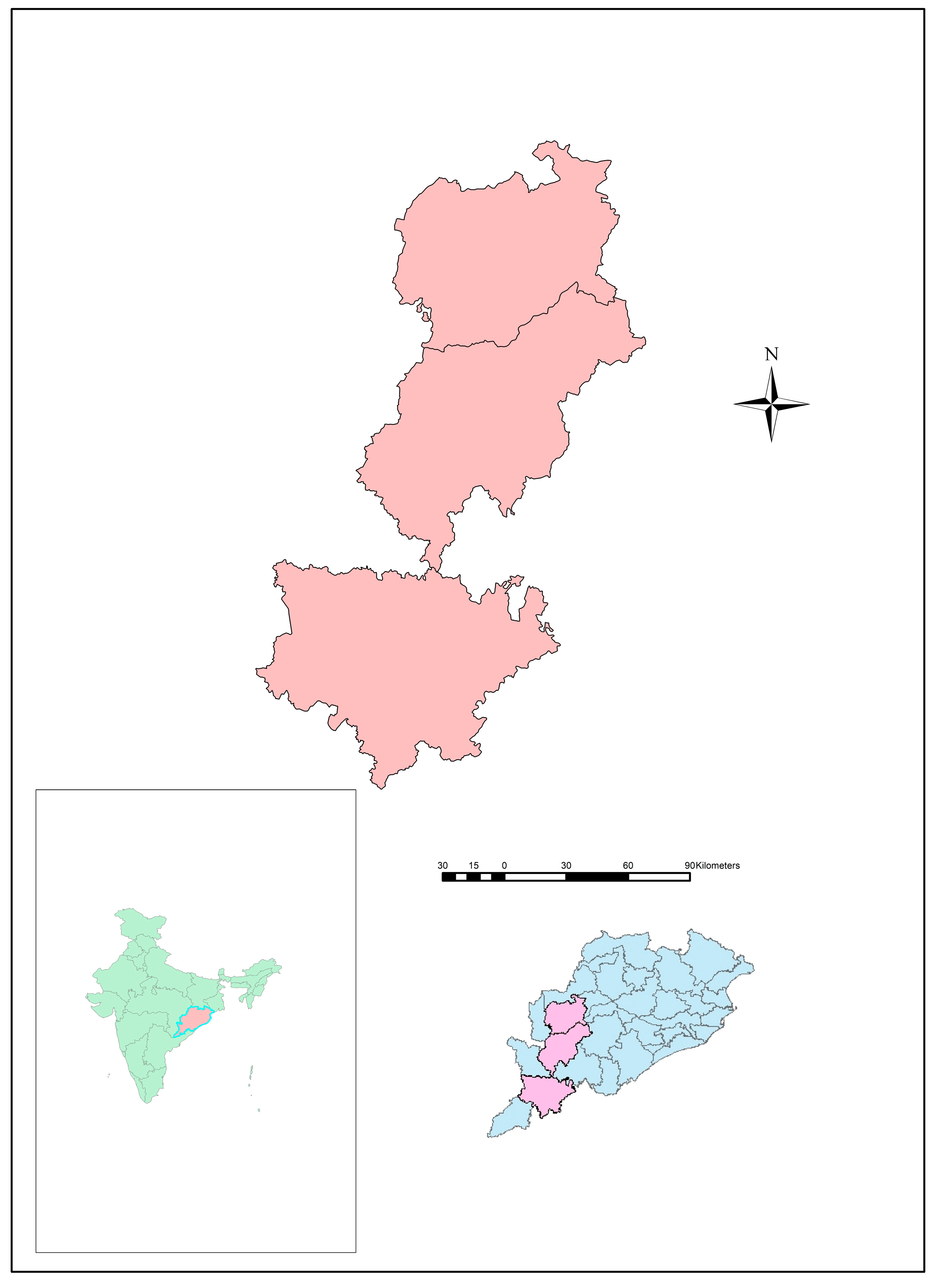
2. Study Area
3. Data Sources and Methodology
3.1. Data Sources
3.2. Methodology
- y: annual crop yield/ area/ rainfall
- y’: anomaly of the variables like crop yield, rainfall, temperature
- y’’: five year running mean
- α = constant
- β = effect/coefficient
- I = dependent
- E = exogenous
3.3. Climatic Indices
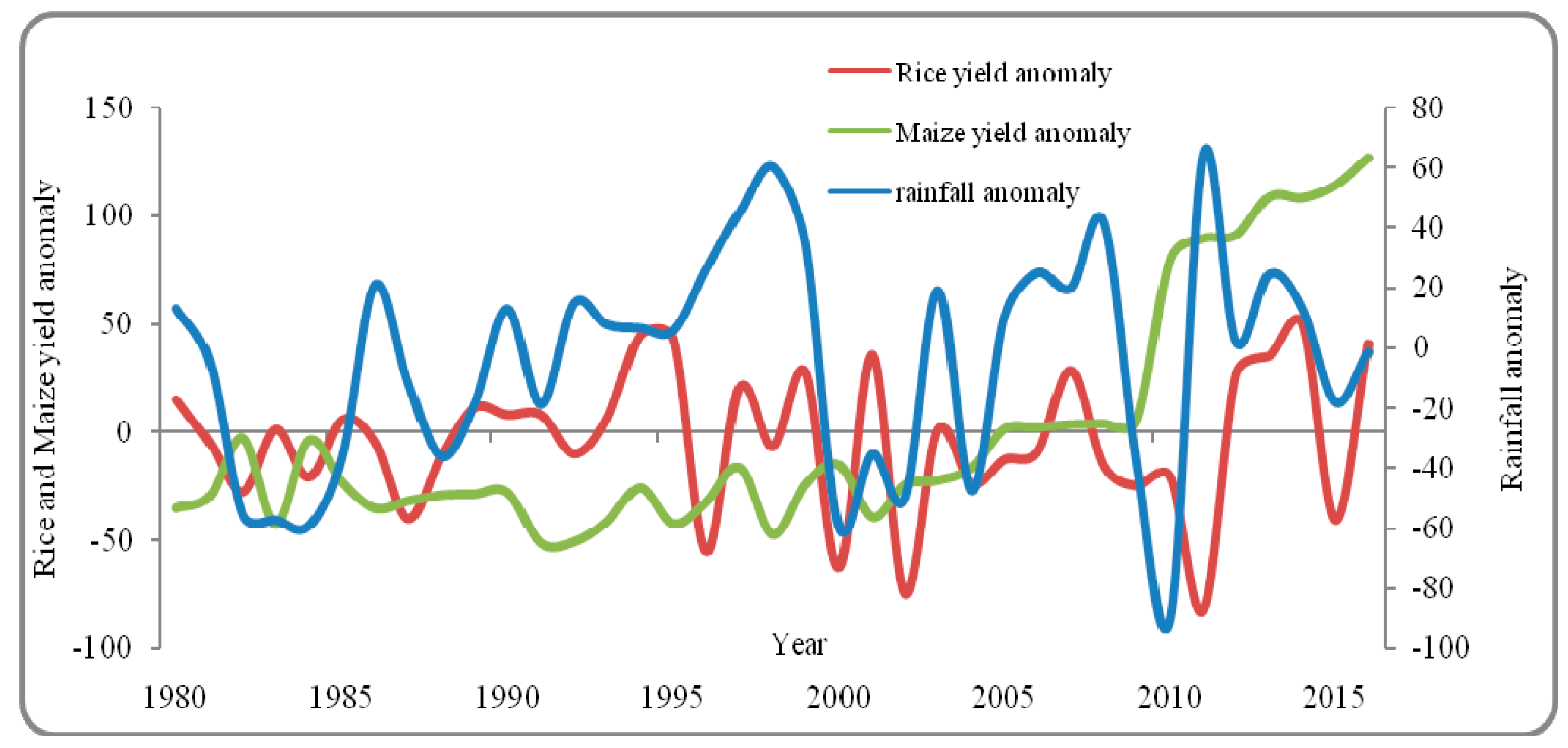
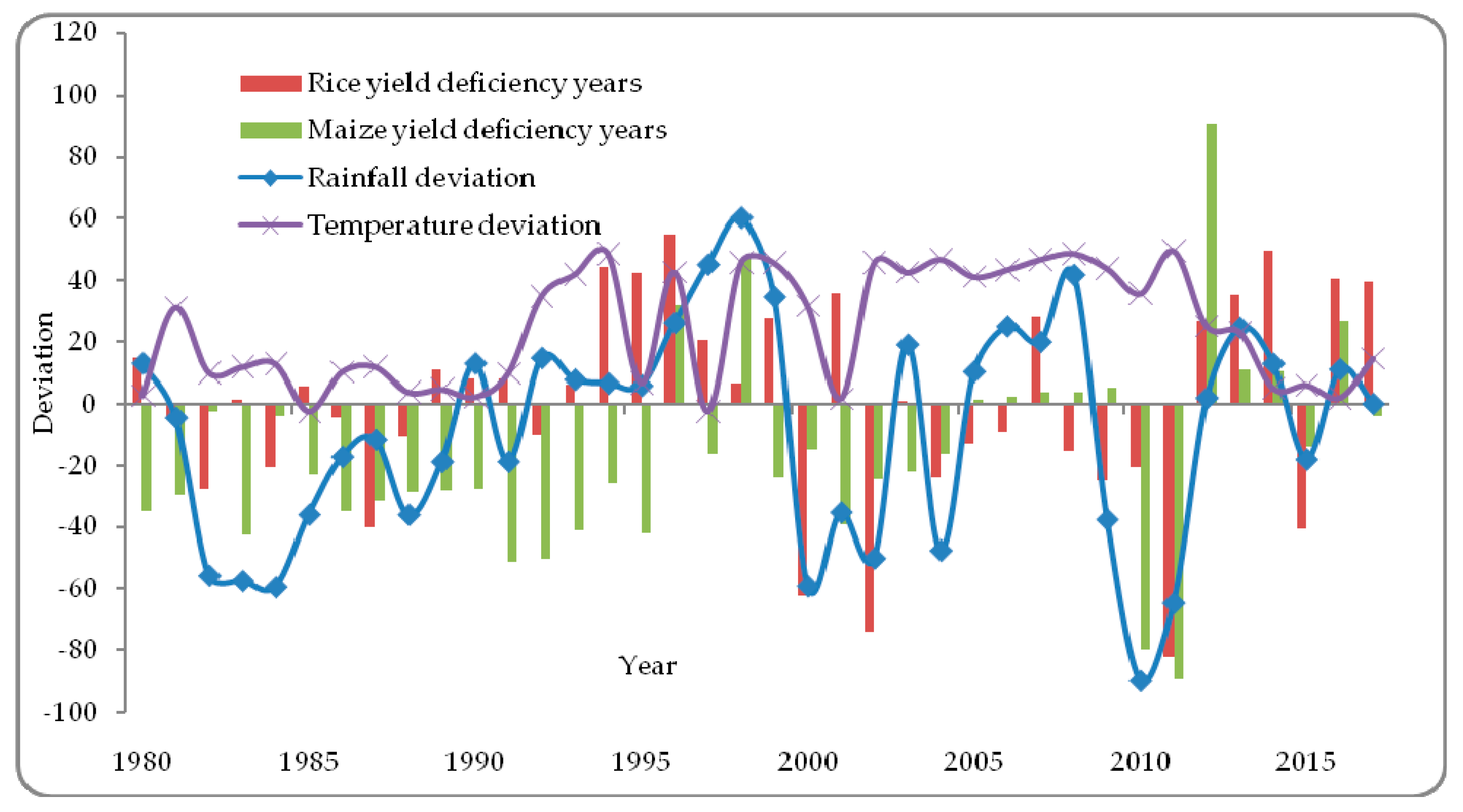
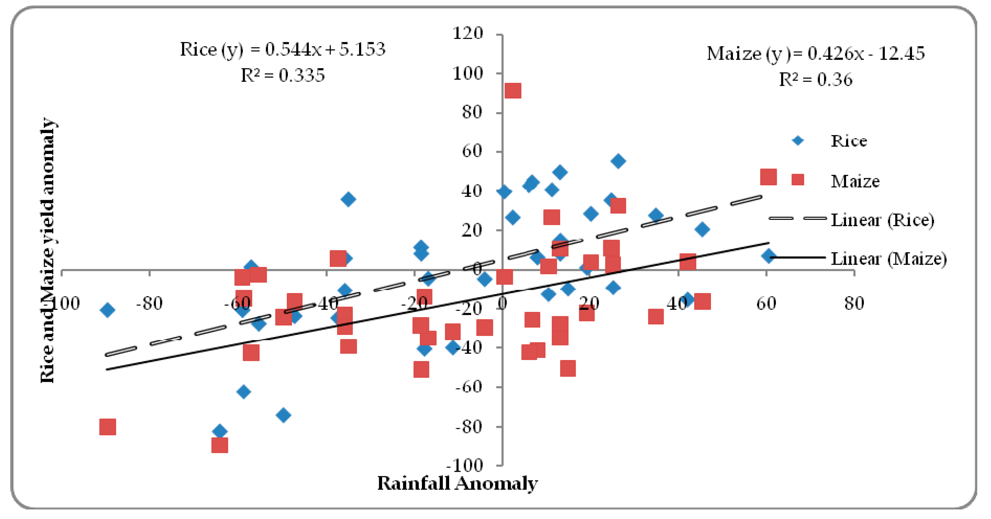
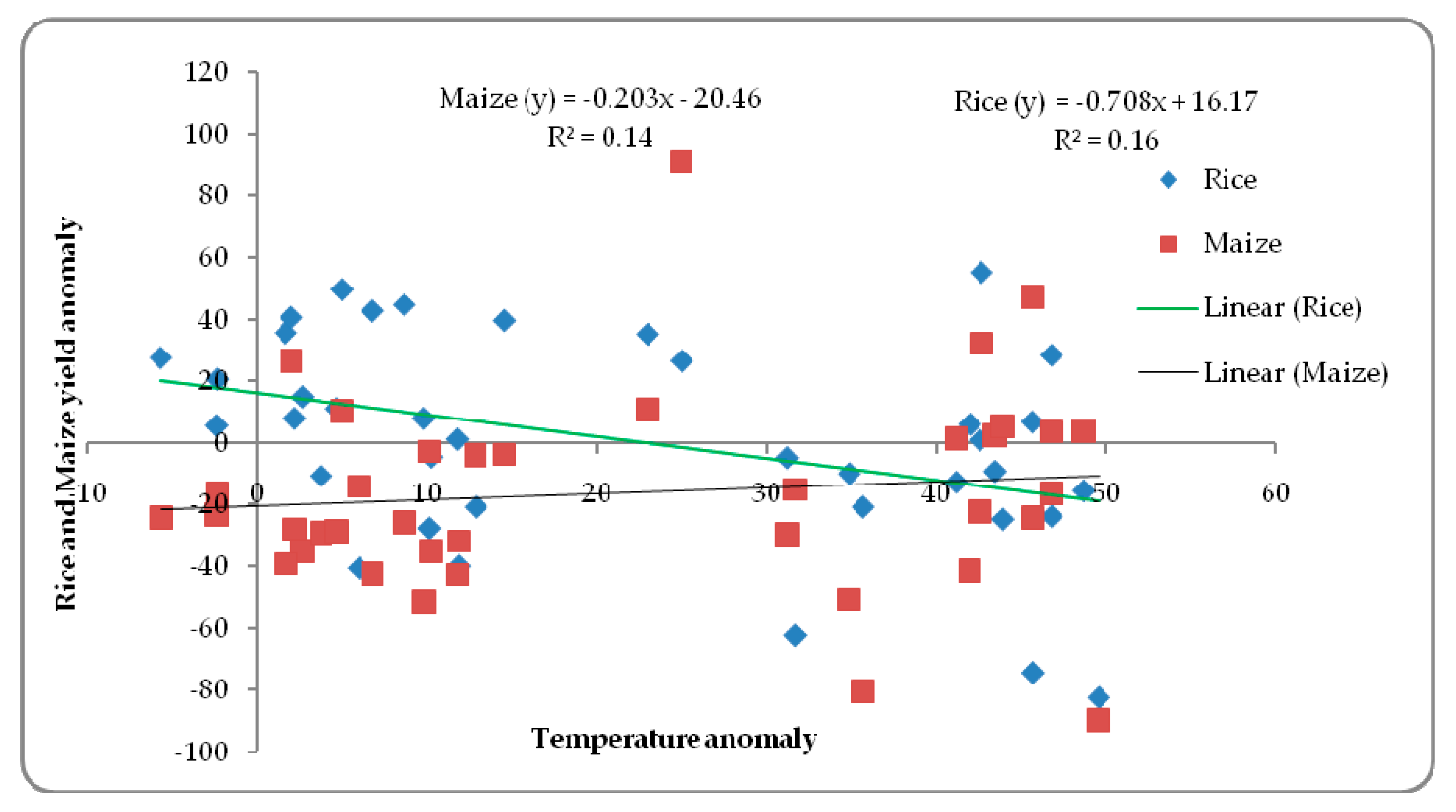
4. Results and Discussion
5. Conclusions
Author Contributions
Funding
Acknowledgments
Conflicts of Interest
References
- Asseng, S.; Cammarano, D.; Anothai, J.; Sanctis, G. Rising Temperatures reduce global Wheat Production. Nat. Clim. Chang. 2015, 5, 143–147. [Google Scholar] [CrossRef]
- De-Graft, H.A.; Kyei, C.K. The Effects of Climatic Variables and Crop Area on Maize Yield and Variability in Ghana. Russ. J. Agric. Socio-Econ. Sci. 2012, 10, 10–13. [Google Scholar]
- Dinar, A.; Mendelsohn, R.; Evenson, R.; Parikh, J.; Sanghi, A.; Kumar, K.; McKinsey, J.; Lonergan, S. Measuring the Impact of Climate Change on Indian Agriculture; Technical Report; The World Bank: Washington, DC, USA, 1998. [Google Scholar]
- Sahu, N.; Yamashiki, Y.; Behera, S.; Takara, K.; Yamagata, T. Large Impacts of Indo-Pacific Climate Modes on the Extremes Streamflows of Citarum River in Indonesia. J. Glob. Environ. Eng. 2012, 17, 1–8. [Google Scholar]
- Sahu, N.; Behera, S.; Yamashiki, Y.; Takara, K.; Yamagata, T. IOD and ENSO Impacts on the Extreme Streamflows of Citarum river in Indonesia. Clim. Dyn. 2012, 39, 1673–1680. [Google Scholar] [CrossRef]
- Egbebiyi, T.S.; Lennard, C.; Crespo, O.; Mukwenha, P.; Lawal, S.; Quagraine, K. Assessing Future Spatio-Temporal Changes in Crop Suitability and Planting Season over West Africa: Using the Concept of Crop-Climate Departure. Climate 2019, 7, 102. [Google Scholar] [CrossRef]
- Egbebiyi, T.S.; Crespo, O.; Lennard, C. Defining Crop-climate Departure in West Africa: Improved Understanding of the Timing of Future Changes in Crop Suitability. Climate 2019, 7, 101. [Google Scholar] [CrossRef]
- De Jager, J.M.; Schulze, R.E. The Broad Geographic Distribution in Natal of Climatological Factors important to Agricultural Planning. Agrochemophysica 1977, 9, 81–91. [Google Scholar]
- Deressa, T. Analysis of Perception and Adaptation to Climate Change in the Nile Basin of Ethiopia. J. Agric. Sci. 2008, 149, 23–31. [Google Scholar] [CrossRef]
- Fisher, G.; Shah, M.; Tubiello, F.; Helhuizen, H. Socio-economic and Climate Change impacts on Agriculture: An Integrated Assessment, 1990–2080. Philos. Trans. R. Soc. B 2005, 360, 2067–2083. [Google Scholar] [CrossRef] [PubMed]
- Gbetiobouo, G.A.; Hassan, R.M. Economic Impact of Climate Change on Major South African Field Crops: A Ricardian Approach. MSc Thesis, Faculty of Natural and Agricultural Sciences, University of Pretoria, Pretoria, South Africa, 2004. [Google Scholar]
- Gbetiobouo, G.A.; Hassan, R.M. Measuring the Economic Impact of Climate Change on Major South African Field Crops: A Ricardian Approach. Glob. Planet. Chang. 2004, 47, 143–152. [Google Scholar] [CrossRef]
- Panda, A.; Sahu, N. Trend Analysis of Seasonal Rainfall and Temperature Pattern in Kalahandi, Bolangir and Koraput Districts of Odisha, India. Atmos. Sci. Lett. 2019. [Google Scholar] [CrossRef]
- Seo, N.; Mendelsohn, R. A Ricardian Analysis of the Impact of Climate Change on South American Farms. Chil. J. Agric. Res. 2008, 68, 69–79. [Google Scholar] [Green Version]
- Loua, T.R.; Bencherif, H.; Mbatha, N.; Begue, N.; Hauchecorne, A.; Bamba, Z.; Sivakumar, V. Study on Temporal Variationsb of Surface Temperature and Rainfall at Conakry Airport, Guinea: 1960–2016. Climate 2019, 7, 93. [Google Scholar] [CrossRef]
- Iizumi, T.; Ramankutty, N. Changes in Yield Variability of Major Crops for 1981–2010 explained by climate change. Environ. Res. Lett. 2016, 11, 034003. [Google Scholar] [CrossRef]
- Cline, W.R. Global Warming and Agriculture: Impact Estimates by Country; Institute of International Economics: Washington, DC, USA, 2007. [Google Scholar]
- Hansen, J.W.; Jones, J.W. El Nino-Southern Oscillation Impacts on Winter Vegetable Production in Florida. J. Clim. 1999, 12, 92–102. [Google Scholar] [CrossRef]
- Census of India. Registrar General & Census Commsisioner, New Delhi. 2011. Available online: http://censusindia.gov.in/2011-Common/CensusData2011.html (accessed on 27 July 2019).
- Kumar, K.K.; Kumar, K.R.; Ashrit, R.G.; Deshpande, N.R.; Hansen, J.W. Climate Impacts on Indian Agriculture. Int. J. Climatol. 2004, 24, 1375–1393. [Google Scholar] [CrossRef]
- Keat, P.; Young, P. Managerial Economics, Economic Tools for Today’s Decision Makers, 3rd ed.; Prentice Hall: Upper Saddle River, NJ, USA, 2000; ISBN 0-13-013538-0. [Google Scholar]
- Wang, B.; Fan, Z. Choice of South Asian Summer Monsoon Indices. Bull. Amer. Meteor. Soc. 1999, 80, 629–638. [Google Scholar] [CrossRef] [Green Version]
- Rajeevan, M.; Azad, S. Possible shift in the ENSO- Indian monsoon rainfall relationship under future global warming. Sci. Rep. 2016, 6, 20145. [Google Scholar]
- Yuan, C.; Yamagata, T. Impacts of IOD, ENSO and ENSO Modoki on the Australian Winter Wheat Yields in Recent Decades. Sci. Rep. 2015, 5, 17252. [Google Scholar] [CrossRef]
- Clark, C.O.; Cole, J.E.; Webster, P.J. Indian Ocean SST and Indian summer rainfall: Predictive relationships and their decadal variability. J. Clim. 2000, 13, 2503–2519. [Google Scholar] [CrossRef]
- Sahu, N.; Singh, R.B.; Kumar, P.; Silva, V.D.; Behera, S. La Nina Imapcts on Austral Summer Extremely High-Streamflow Events of the Paranaiba River in Brazil. Adv. Meteorol. 2013. [Google Scholar] [CrossRef]
- Sahu, N.; Singh, R.B.; Duan, W.; Silva, V.D.; Behera, S.; Ratnam, J.V. El Nino Modoki Connection to Extremely-low Streamflow of the Paranaiba river in Brazil. Clim. Dyn. 2014, 42, 1509–1516. [Google Scholar] [CrossRef]
- Sahu, N.; Singh, R.B.; Kumar, M.; Behera, S.; Takara, K. Probabilistic Seasonal Streamflow Forecats of the Citarum river, Indonesia, based on General Circulation Models. Stoch. Environ. Res. Risk Assess. 2016. [Google Scholar] [CrossRef]
- Pandey, V.; Sharma, A.; Bharati, L.; Joshi, I.; Dhaubanjar, S. Climate Shocks and Responses in Karnali- Mahakali Basins, Western Nepal. Climate 2019, 7, 92. [Google Scholar] [CrossRef]
- Meshram, S.G.; Singh, S.K.; Meshram, C.; Deo, R.C.; Ambade, B. Statistical evaluation of rainfall time series in concurrence with agriculture and water resources of Ken River basin, Central India (1901–2010). Theor. Appl. Climatol. 2018, 134, 1231–1243. [Google Scholar] [CrossRef]
- Nayak, S.; Mandal, M. Impact of land use and land cover changes on temperature trends over western India. Curr. Sci. 2012, 102, 1166–1173. [Google Scholar]
- Nayak, S.; Mandal, M. Examining the impact of regional land use and land cover changes on temperature: The case of Eastern India. Spat. Inf. Res. 2019. [Google Scholar] [CrossRef]
- Schelenker, W.; Lobell, B.D. Robust Negative Impacts of Climate Change on African Agriculture. Environ. Res. Lett. 2010, 5. [Google Scholar] [CrossRef]
- Morton, J.F. The Impact of Climate Change on Smallholder and Subsistence Agriculture. Proc. Natl. Acad. Sci. USA 2007, 104, 19680–19685. [Google Scholar] [CrossRef]


| Rainfall Deviation Years > 10% | Temperature Deviation Years > 10% | Rice Yield Deficient Years > 10% | Maize Yield Deficient Years > 10% | ||||
|---|---|---|---|---|---|---|---|
| 1982 | −25.44 | 1981 | 31.22 | 1982–3 | −33.11 | 1981–82 | −23.12 |
| 1983 | −37.46 | 1985 | 10.12 | 1984–85 | −23.31 | 1983–84 | −21.32 |
| 1984 | −29.34 | 1986 | 11.81 | 1987–88 | −43.61 | 1984–85 | −39.60 |
| 1987 | −18.55 | 1989 | 12.89 | 1988–89 | −14.70 | 1988–89 | −17.80 |
| 1988 | −32.57 | 1992 | 10.23 | 1996–97 | −57.40 | 1991–92 | −46.21 |
| 1990 | −10.23 | 1995 | 11.90 | 2000–01 | −62.79 | 2000–01 | −24.68 |
| 1991 | −14.32 | 1998 | 13.76 | 2002–03 | −75.67 | 2003–04 | −31.90 |
| 2000 | −55.32 | 2003 | 24.68 | 2004–05 | −21.34 | 2006–7 | −19.60 |
| 2001 | −22.78 | 2006 | 32.20 | 2008–09 | −11.88 | 2012–13 | −47.08 |
| 2002 | −40.07 | 2012 | 29.80 | 2009–10 | −18.81 | 2014–15 | −66.59 |
| 2004 | −45.99 | 2014 | 34.87 | 2010–11 | −26.52 | 2016–17 | −77.67 |
| 2005 | −24.84 | 2015 | 41.98 | 2011–12 | −87.23 | ||
| 2009 | −42.65 | 2016 | 38.65 | 2015–16 | −41.43 | ||
| 2010 | −90.07 | ||||||
| Rice Yield (Rainfall Anomaly) | Maize Yield (Rainfall Anomaly) | |
|---|---|---|
| Multiple R | 0.856 | 0.738 |
| R2 | 0.732 | 0.544 |
| Beta | 0.856 | 0.738 |
| Sig | 0.018 | 0.044 |
| Monsoon Index (MI) | Rice | Maize | ||
|---|---|---|---|---|
| Yield | Production | Yield | Production | |
| MI-JJA | 0.61 | 0.50 | 0.55 | 0.49 |
| MI-JAS | 0.66 | 0.54 | 0.59 | 0.51 |
| MI-JJAS | 0.60 | 0.55 | 0.56 | 0.43 |
| Rice Yield (MI-JJA) | Rice Yield (MI-JJAS) | Maize Yield (MI-JJA) | Maize Yield (MI-JJAS) | |
|---|---|---|---|---|
| R | 0.65 | 0.51 | 0.56 | 0.48 |
| R2 | 0.42 | 0.26 | 0.31 | 0.23 |
| Beta | 0.65 | 0.51 | 0.56 | 0.48 |
| Sig | 0.013 | 0.023 | 0.034 | 0.04 |
| ONI | NINO-3 | NINO-3.4 | |||||
|---|---|---|---|---|---|---|---|
| NDJ | DJF | NDJ | DJF | NDJ | DJF | ||
| Rice | Yield | 0.39 | 0.42 | 0.32 | 0.39 | 0.32 | 0.35 |
| Production | 0.35 | 0.38 | 0.32 | 0.34 | 0.34 | 0.36 | |
| Maize | Yield | 0.41 | 0.43 | 0.39 | 0.33 | 0.38 | 0.39 |
| Production | 0.36 | 0.39 | 0.40 | 0.34 | 0.38 | 0.36 | |
© 2019 by the authors. Licensee MDPI, Basel, Switzerland. This article is an open access article distributed under the terms and conditions of the Creative Commons Attribution (CC BY) license (http://creativecommons.org/licenses/by/4.0/).
Share and Cite
Panda, A.; Sahu, N.; Behera, S.; Sayama, T.; Sahu, L.; Avtar, R.; Singh, R.B.; Yamada, M. Impact of Climate Variability on Crop Yield in Kalahandi, Bolangir, and Koraput Districts of Odisha, India. Climate 2019, 7, 126. https://0-doi-org.brum.beds.ac.uk/10.3390/cli7110126
Panda A, Sahu N, Behera S, Sayama T, Sahu L, Avtar R, Singh RB, Yamada M. Impact of Climate Variability on Crop Yield in Kalahandi, Bolangir, and Koraput Districts of Odisha, India. Climate. 2019; 7(11):126. https://0-doi-org.brum.beds.ac.uk/10.3390/cli7110126
Chicago/Turabian StylePanda, Arpita, Netrananda Sahu, Swadhin Behera, Takahiro Sayama, Limonlisa Sahu, Ram Avtar, R.B. Singh, and Masafumi Yamada. 2019. "Impact of Climate Variability on Crop Yield in Kalahandi, Bolangir, and Koraput Districts of Odisha, India" Climate 7, no. 11: 126. https://0-doi-org.brum.beds.ac.uk/10.3390/cli7110126