Air Pollution Flow Patterns in the Mexico City Region


Instituto Nacional de Electricidad y Energías Limpias, Reforma 113, Palmira, Cuernavaca 62490, Morelos, Mexico
*
Author to whom correspondence should be addressed.
Climate 2019, 7(11), 128; https://0-doi-org.brum.beds.ac.uk/10.3390/cli7110128
Submission received: 18 September 2019
/
Revised: 22 October 2019
/
Accepted: 31 October 2019
/
Published: 5 November 2019
(This article belongs to the Special Issue Urban Climate and Adaptation Tools)
Abstract
:According to the Mexico City Emissions Inventory, mobile sources are responsible for approximately 86% of nitrogen oxide emissions in this region, and correspond to a NOx emission of 51 and 58 kilotons per year in Mexico City and the State of Mexico, respectively. Ozone levels in this region are often high and persist as one of the main problems of air pollution. Identifying the main scenarios for the transport and dispersion of air pollutants requires the knowledge of their flow patterns. This work examines the surface flow patterns of air pollutants (NO2, O3, SO2, and PM10) in the area of Mexico City (a region with strong orographic influences) over the period 2001–2010. The flow condition of a pollutant depends on the spatial distribution of its concentration and the mode of wind circulation in the region. We achieved the identification and characterization of the pollutant flow patterns through the exploitation of the 1-hour average values of the pollutant concentrations and wind data provided by the atmospheric monitoring network of Mexico City and the application of the k-means method of cluster analysis. The data objects for the cluster analysis were obtained by modeling Mexico City as a 4-cell spatial domain and describing, for each pollutant, the flow state in a cell by the spatial averages of the horizontal pollutant flow vector and its gradients (the divergence and curl of the flow vector). We identified seven patterns for wind circulation and nine patterns for each of NO2, O3, PM10, and SO2 pollutant flows. Their seasonal and annual average intensities and probabilities of occurrence were estimated.
1. Introduction
In cities and large urban settlements, tropospheric ozone and particulate matter (PM10 and PM2.5) are the most dangerous air pollutants for human health [1]. Air pollution is a major environmental issue in urban areas, which can affect the well-being and quality of life of citizens. More and more frequently, there are detected chronic diseases of great importance that are associated with continuous exposures to high concentrations of air pollutants. Epidemiological studies have reported that exposure to air pollutants such as particulate matter, nitrogen oxides (NOx), sulfur dioxide (SO2), and surface ozone (O3) associates with an increase in mortality and hospital admissions predominantly related to respiratory and cardiovascular diseases [1,2]. This critical issue concerns the 20 million people (including 9 million children) living in the Mexico City Metropolitan Area (MCMA). Despite the reductions in the emissions of common air pollutants in MCMA since the early 1990s, millions of people remain exposed to concentrations above the critical levels associated with increased risks for cardiovascular and respiratory diseases. The anthropogenic sources still produce and release to the atmosphere every year large amounts of carbon monoxide (CO), nitrogen oxides (NOx), sulfur dioxide (SO2), particulate matter (PM10 and PM2.5), and volatile organic compounds (VOC) [3]. However, because of the frequency of occurrence of high levels, persistence, and spatial distribution, the most critical air pollutants in MCMA are by far ozone and PM10 [4,5,6].
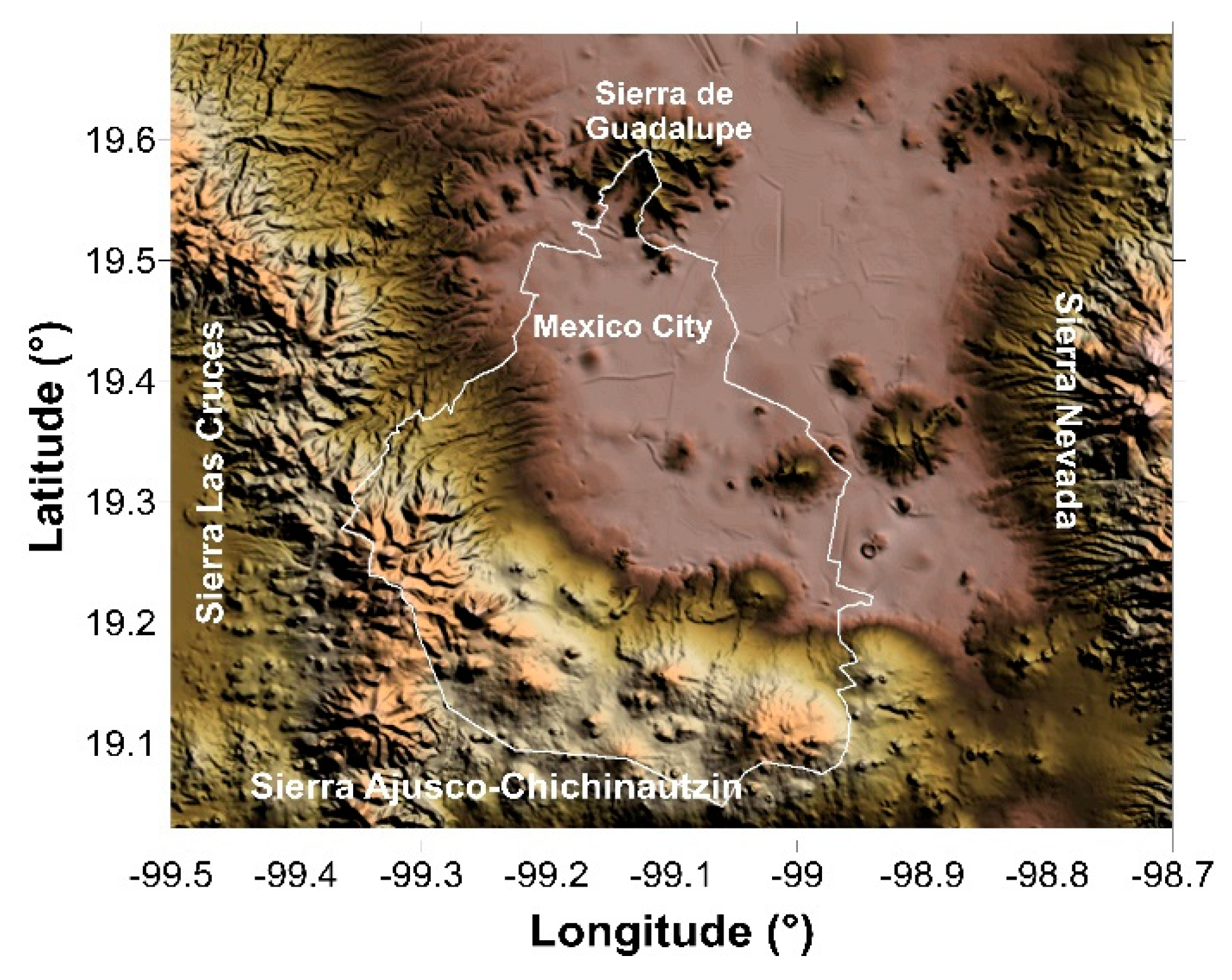
At the MCMA, the complexity of the air pollution problem is also strongly related to other essential factors such as the geographical setting, meteorology, and topography. MCMA lies inside a subtropical basin with latitudes between 19.2 and 19.6 °N and longitudes between 98.9 and 99.4 °W, and an average altitude of 2240 m, surrounded by high mountains (Figure 1). In the north direction, the basin extends into the Mexican plateau and the arid interior of the country, with the Sierra de Guadalupe creating a small 800 m barrier above the basin floor. Its climate classification comprises two seasons: the rainy season from May to October and the dry season from November to April. This classification stems from the two main meteorological patterns on the synoptic-scale: dry westerly winds with anticyclone conditions from November until April, and moist flows from the east due to the weaker trade winds along the other six months [7]. The MCMA meteorology, however, is by far more complicated than this simple classification expresses it. The basin interacts with the Mexican plateau and the lower coastal areas. Moreover, due to the MCMA location, large-scale pressure gradients are generally weak, and intense solar radiation is registered here throughout the year [7,8,9,10,11]. These conditions and the presence of high mountains in the surroundings are ideal for the development of thermally driven winds.
The knowledge of wind circulation and air pollutant spatial distributions constitutes a relevant element to understand the flow dynamics of urban air pollution. It allows knowing how the air pollutant emissions produced in an urban settlement may disperse in the atmosphere, how these air pollutants may be distributed spatially in the city, and how the winds may transport them towards neighboring sites [12,13]. From the standpoint of fluid dynamics, the pollutant-flow vector, defined as the product of the fields of the pollutant concentration and wind velocity,
describes the transport of a given pollutant in the atmosphere. Then, the surface flow condition of a pollutant depends on both factors: the surface distribution of its concentration and the local wind circulation.
Local wind circulation in Mexico City and its relation to driving forces and air pollution have been studied extensively for almost three decades. However, most of the studies have been performed on an episode-by-episode basis and using small data sets obtained from short-term experimental campaigns with different approaches [14,15,16,17,18,19,20,21]. Some of the main exceptions are the first long-term micrometeorological campaign carried out by Salcido et al. [11] in this region during 2001, and the studies of Klaus et al. [22], de Foy et al. [23], Salcido et al. [24], and Carreón-Sierra et al. [25], which were carried out using data provided by the atmospheric monitoring network of Mexico City (SIMAT: Sistema de Monitoreo Atmosférico de la Ciudad de México [26]). Klaus et al. [22] reported a principal component analysis of air quality and meteorological data for the period February–December 1995. The study of de Foy et al. [23] reported an examination of wind transport during the experimental campaign of the Megacity Initiative: Local and Global Research Observations (MILAGRO) project; they used cluster analysis for making a comparison to climatology between the period of March 2006 and the period 1998–2006 using hourly wind data of the warm, dry season. In their work, Salcido et al. [24] used a lattice wind model at a meso-β scale to carry out a description and characterization of Mexico City local wind events of the period 2001–2006. Furthermore, Carreón-Sierra et al. [25] proposed an extension of the local wind state using a non-local description based on the wind velocity and its gradients and applied hierarchical cluster analysis to recognize and characterize the Mexico City wind circulation patterns in the period 2001–2006. As far as we know, the last paper reported the first work where a non-local approach is used to characterize the wind condition for identifying patterns with more detail than the simple results produced by the wind rose method.
In this paper, extending our previous work [25], we examine the main surface patterns of wind circulation and pollutant-flow of NO2, O3, SO2, and PM10 in the Mexico City region over the period 2001–2010. We achieved the identification and characterization of the pollutant-flow patterns through the exploitation of the 1-hour average values of the pollutant concentrations and wind data provided by the atmospheric monitoring network of Mexico City (SIMAT [26]) and the application of cluster analysis as a data mining procedure. First, we considered Mexico City as a 2D lattice domain and defined the flow condition (or flow state) of a given pollutant in each lattice cell in terms of a flow vector field and its gradients (precisely, the divergence and curl of this flow vector). Second, we used the 1-h average values of the pollutant concentrations and wind data provided by SIMAT to estimate, using Kriging interpolation, discrete representations of the pollutant-flow vector field and its gradients over the lattice domain. Finally, we used the k-means method of cluster analysis [27,28,29] to identify and characterize the pollution-flow patterns from the clustering modes of the flow states. We identified seven patterns for wind circulation and nine patterns for each of NO2, O3, PM10, and SO2 pollutant-flows. Their seasonal and annual average intensities and probabilities of occurrence were also estimated.
2. Materials and Methods
In this section, we detail the study domain, data, and procedure that we used to identify and characterize the wind and pollution-flow patterns.
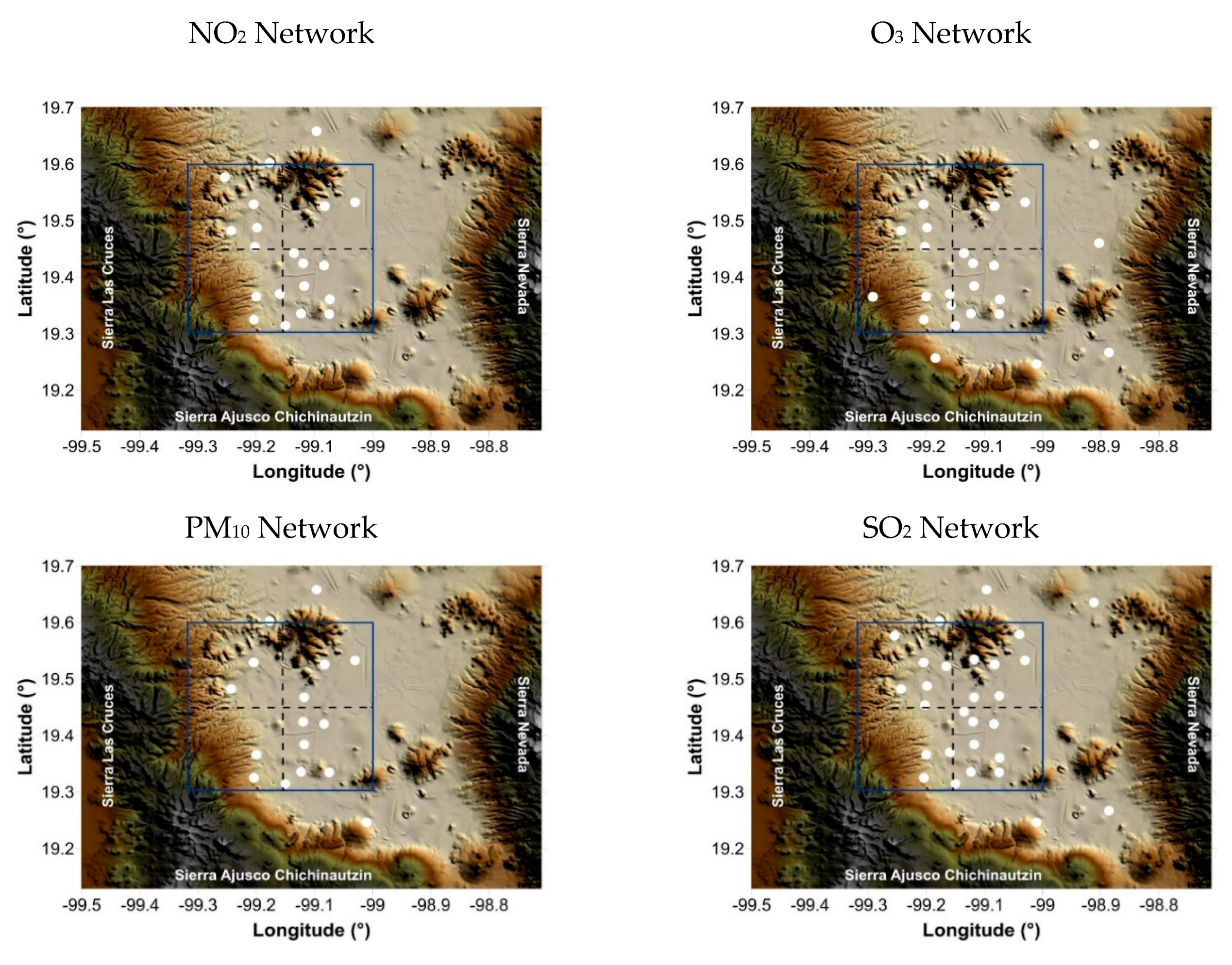
2.1. Study Domain
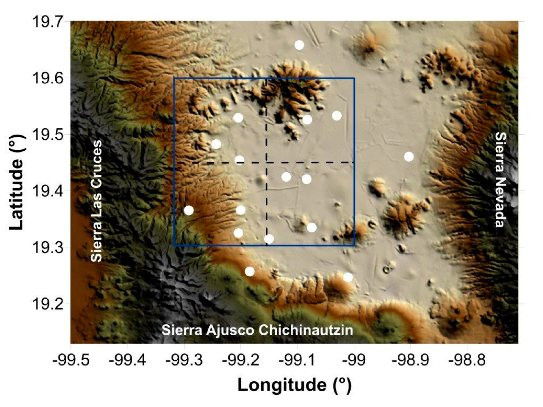
We considered the part of Mexico City located at 19.3°–19.6°N and 99.0°–99.3°W as the study domain. In Figure 2, we showed this region as enclosed by a solid line square. This region contains 75% of the stations of the wind-monitoring network (REDMET) of SIMAT, 95% of the NO2 stations, 83% of the O3 stations, 93% of the PM10 stations, and 86% of the SO2 stations of the air quality monitoring network (RAMA) of SIMAT (Figure 3). Because of the topographic complexity of the mountains surrounding Mexico City, we examined the pollutant flows in this region, assuming it divided into quadrants (NE, NW, SW, and SE). We defined these quadrants using a reference frame with origin at (19.43°N, 99.13°W) and the axes along the west to east (W–E) and south to north (S–N) directions (dotted lines in Figure 2). The origin of the reference frame is the geometric centroid of the REDMET stations. The positions of the geometric centers of the city quadrants are: (19.5°N, 99.1°W), (19.5°N, 99.2°W), (19.4°N, 99.2°W), and (19.4°N, 99.1°W) for the NE, NW, SW, and SE quadrants. The dimensions of each quadrant were 15.66 km length in the west–east direction and 16.56 km length in the south–north direction (each quadrant is a square of 540 × 540 arcsec). In principle, we expect to detect the ventilation effects due to the openings located at the west and east sides of the Sierra de Guadalupe (north of the city) at NW and NE quadrants, respectively, and to observe in the SE quadrant the effect of the gap situated in the southeast of the Mexico basin. Also, in the SE and NE quadrants, we expect to recognize the effects of the winds blowing along the ventilation channel determined by the volcanos (Sierra Nevada) on the east side of the city. Moreover, we expect to recognize the wind effects due to the Mexico City mountain-valley system in all quadrants, but mainly in the NW and SW quadrants.
2.2. Data
Figure 2 and Figure 3 illustrate the study domain and the spatial distributions of the stations of the monitoring networks of SIMAT for wind, nitrogen dioxide, ozone, PM10, and sulfur dioxide. These monitoring networks provided the 1-hour average values of the meteorological and air quality variables systematically and made them publicly available through its web site [26]. For the present work, we collected the wind data (wind speed and wind direction) and the air quality data (NO2, O3, PM10, and SO2 surface concentrations) for the period 2001–2010, which constitute a database with 87,600 records, approximately, for each hourly averaged variable.
2.3. Study Database
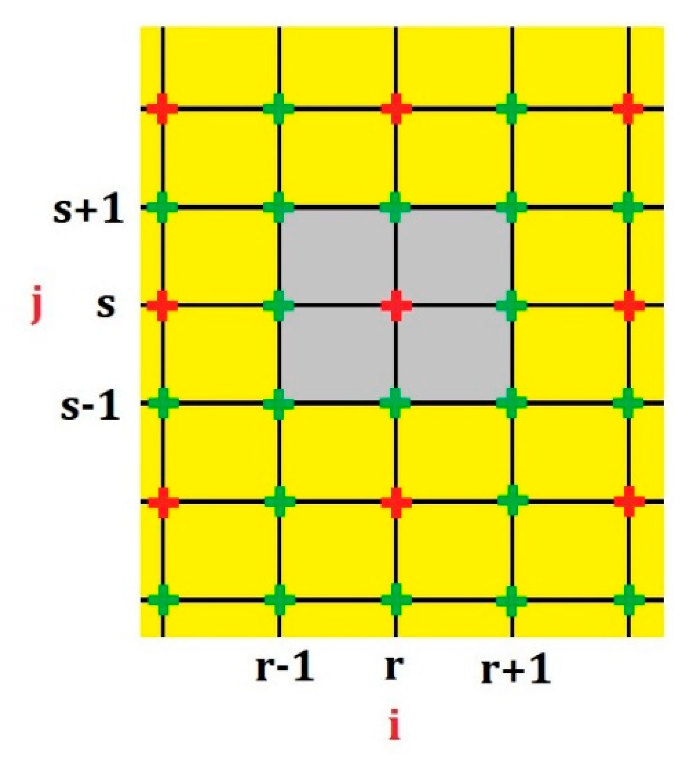
In a first step, we represented the study domain (D) as a square grid G with 289 nodes Grs, where the subscripts r = 1, 2, …, 17 and s = 1, 2, …, 17 vary along with the West–East (WE) and South–North (SN) directions, respectively. Using the wind speed and wind direction data supplied by the REDMET stations, and the NO2, O3, PM10, and SO2 concentration data supplied by the RAMA stations, we estimated (using Kriging interpolation) the horizontal components of the flow vector field at each grid node Grs and time t,
For a given pollutant, at the node Grs and time t, is the pollutant concentration, and and are the wind velocity components. Here, time t is an integer running from 1 to the number H of hours (87,600, approximately) in the period 2001–2010.
Then, we defined a 2D lattice L composed by 64 regular non-overlapping cells Cij covering D, with i = 1, 2, 3, …, 8 and j = 1, 2, 3, …, 8, such that each cell Cij is surrounded by nine grid nodes of G, as Figure 4 illustrates it.
The estimations, for each pollutant, of the flow vector components at the grid nodes Grs, allow calculating (numerically) the spatial averages of the components of the pollutant-flow vector and its gradients at the cells Cij of the lattice L using their 2D discrete definitions in terms of centered finite differences [24,30]. For a given pollutant, we will denote the flow vector components at Cij by and , and the associated divergence and curl of the flow vector will be denoted by and . Here, x and y denote the WE and SN directions, respectively. At this level, we will be referring to this non-local discrete representation of the flow condition of the study domain as the 64-cell model. It involves 256 (= 4 × 64) parameters to define an event of the system (i.e., to describe the flow condition over the complete spatial domain). In this work, for simplicity in the handling and interpretation of the results, we considered the reduction of the 64-cell model to the cases of the 4-cell and 1-cell models, which we obtained using a spatial averaging procedure. In any case, the four parameters (jx, jy, Γ, Ω) define the flow state at a lattice cell; therefore, the 4-cell and 1-cell models respectively entail 16 and 4 parameters to describe an event of the system. It is convenient to note that the introduction of the additional variables (Γ, Ω) in the flow state definition, allows recovering some of the information lost during the spatial averaging of the flow vector components. This assumption gives a slight non-local character to this description [31].
For each cell Cij, we calculated, hour by hour, the average of the four state-variables over the 2001–2010 period, defining a one generic year database for each pollutant and cell model considered. The results were normalized and then organized in seasonal groups: January–March (winter), April–June (spring), July–September (summer), and October–December (autumn).
We performed data normalization as follows. We determined the maximum absolute values of the magnitude of the pollutant-flow vector |j|max, and the divergence |Γ|max, and curl |Ω|max of the flow vector, in the generic year database. Then the normalized and dimensionless state variables (all of them now ranging in the interval [−1, +1]) were calculated using the following expressions:
2.4. Clustering Method
We used the k-means method of cluster analysis as a procedure of data mining to identify and characterize the main patterns of wind and flow of pollutants in the Mexico City region.
Cluster analysis comprises a broad set of techniques for finding non-overlapping subgroups of data objects in a dataset. When clustering the data objects of a dataset, we seek to organize them into a given number of distinct subsets (groups, or clusters), so that they constitute a partition of the initial dataset; this way, the data objects within each subset are quite similar to each other, while data objects in different groups are quite different from each other [29]. Clustering is an unsupervised problem because we are trying to discover structure (distinct clusters) based on a dataset, without being trained by a response variable.
The k-means clustering method is the simplest and the most frequently used technique of cluster analysis for partitioning a dataset into a set of k groups. In k-means clustering, we seek to partition the set of data objects into a pre-specified number of clusters, so that the total within-cluster variation (TWCV) is as small as possible.
Suppose we have a dataset and we try to partition X into M disjoint clusters C1, C2, CM. Then, the k-means algorithm detects local optimal solutions concerning the TWCV defined as the sum of squared Euclidean distances between each data object xi and the centroid mk of the cluster Ck that contains xi. Analytically, the TWCV is given by
where if and 0 otherwise. The TWCV measures the clustering goodness, and the optimization problem that defines the k-means clustering resides in minimizing TWCV. In practice, we used the software DataLab developed by Hans Lohninger [32] to perform the cluster analysis with the k-means algorithm.
For each air pollutant considered, we define its set of data objects as
where T = 8760 is the number of hours of the generic year, and
with Nx = 2 (Nx = 1) and Ny = 2 (Ny = 1) in the case of the 4-cell (1-cell) model. We organized the dataset H in the seasonal subsets Hwinter, Hspring, Hsummer, and Hautumn comprising, respectively, the data objects of the periods January–March (winter), April–June (spring), July–September (summer), and October–December (autumn). We identified each data object of these subsets with a label of the form MMDDHH that specifies the date (relative to the generic year) and hour of occurrence.
To carry out the cluster analysis for each seasonal period, we build a data matrix structured as described in Table 1.
For each pollutant, using the respective data matrixes of the seasonal subsets, we can apply the k-means algorithm for clustering the associated data objects considering the parameters of the 1-cell or 4-cell model as the clustering variables. Although we can expect that the 4-cell model variables will produce a physically more detailed clustering of the wind and pollutant-flow events, in this work, for easiness in handling the results, we used only the 1-cell model parameters as clustering variables. The application of the clustering procedure to the 1-cell model data objects will organize them, assigning the cluster number to the date-time labels that identify the events. Consequently, the 4-cell model data objects also receive cluster numbers correspondingly. It means that the data objects of the 4-cell model were also organized into clusters by the same clustering procedure. Therefore, for each pollutant and seasonal period, we have clusters of events characterized by the sixteen parameters of the 4-cell model:
where C0, C1, C2, and C3 are the cells of the model.
2.5. The Number of Clusters
The k-means clustering is a simple and fast algorithm that can efficiently deal with large datasets. However, the k-means approach requires pre-specifying the number of clusters; and preferably, we would like to use an optimal number of clusters that we defined according to some given criterion. In this work, because of the motivation expressed in the following two paragraphs, we applied the k-means clustering method to organize each seasonal period in six clusters of data objects (events).
2.5.1. Physical Motivation
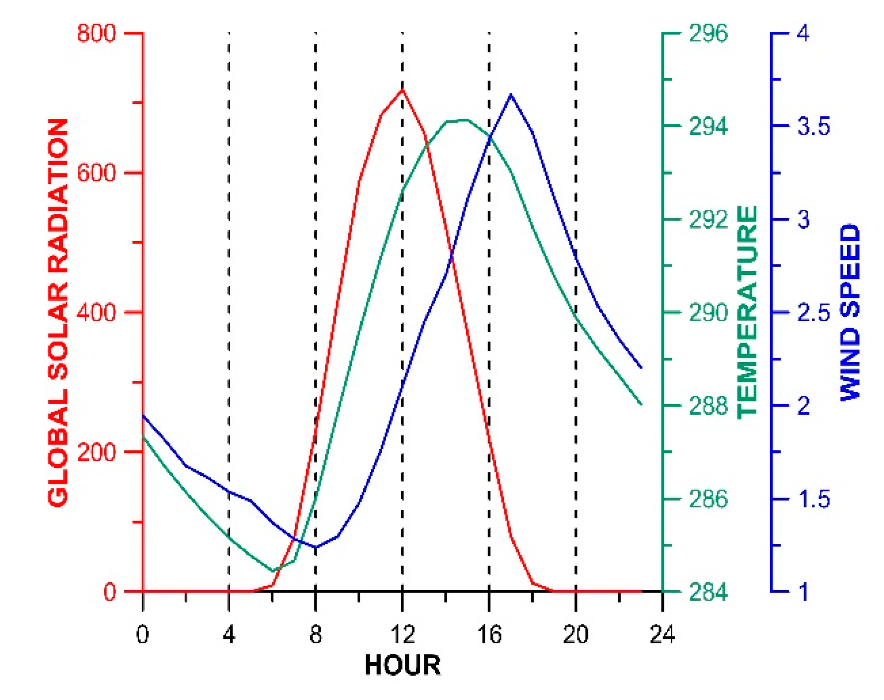
In Figure 5, we presented the mean diurnal behavior of solar radiation, temperature, and wind speed observed during 2001. We obtained these results from data we measured at an urban site southeast Mexico City (Xochimilco) [11,25]. The plots evidence that the meteorological events comprised in the six time-periods 0–4, 4–8, 8–12, 12–16, 16–20, and 20–24 h, are quite different from each other. The periods 0–4 and 20–24 h show the cooling phase of the atmosphere during the night. In the period 4–8 h, we observe the sunrise occurrence, and that temperature and wind speed reach their minimum values. The period 8–12 h shows the growing phases of solar radiation, temperature, and wind speed, with solar radiation reaching its maximum. The period 12–16 h depicts the temperature reaching its maximum, while wind speed keeps growing, and solar radiation starts to decrease. Finally, the period 16–20 h shows the sunset occurrence, the wind speed reaching its maximum, and temperature decreasing. Appreciation of these different behaviors suggests searching for six groups during the application of the k-means algorithm for clustering the data objects defined by the events of wind circulation and pollutant-flow in Mexico City.
2.5.2. The Elbow Method
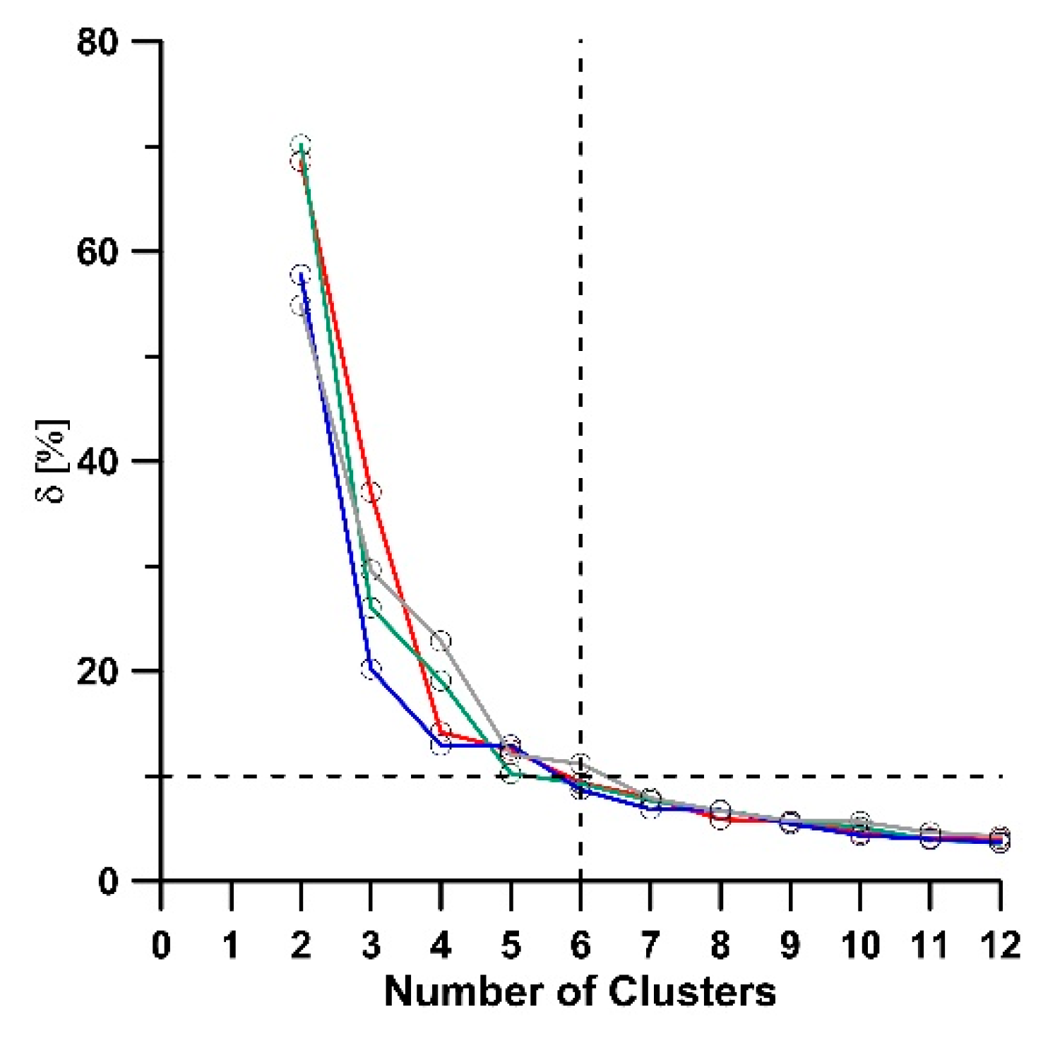
From the standpoint of cluster analysis, one of the most popular methods for determining the optimal clusters is the elbow method. It provides a simple solution. The basic idea is to compute the k-means clustering algorithm using different numbers, k, of clusters. The next step is drawing the total within-cluster variation (or total within-cluster sum of squares) versus the number of clusters. Commonly, the analysts consider the location of a bend in the plot as an indicator of the appropriate number of clusters. However, it is not always clear where the bend point position is. We preferred to calculate the percentage reduction (δ) of the total within-cluster sum of squares of a given k, relative to its value for the previous number of clusters k − 1, and then to plot δ as a function of k. As our optimal number of clusters, we selected the value of k from which on the reduction δ is less than 10% each unit step in increasing k. For example, according to this procedure, Figure 6 shows that we must select k = 6 when clustering the winter wind data objects of the present work.
3. Results and Discussion
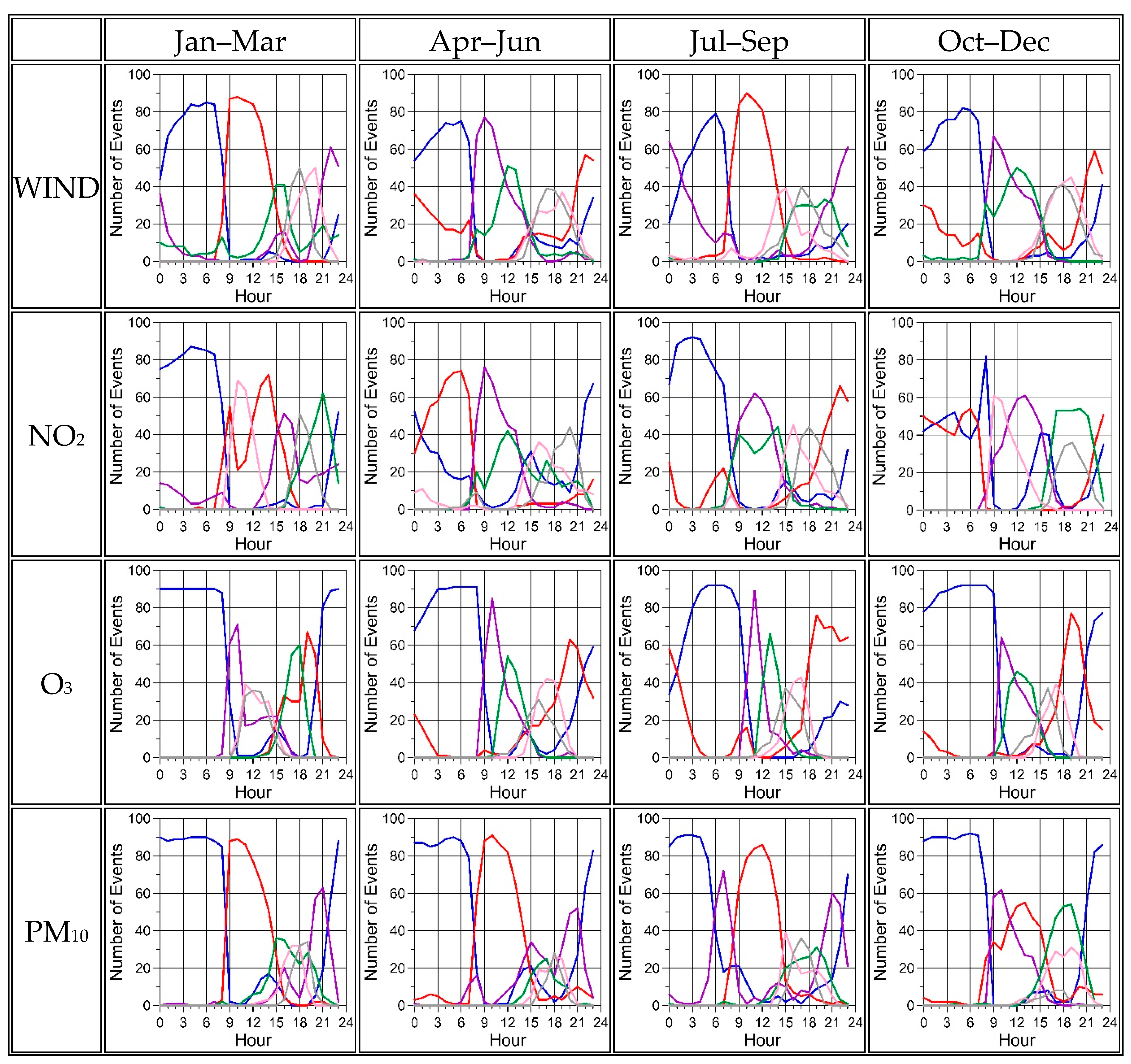
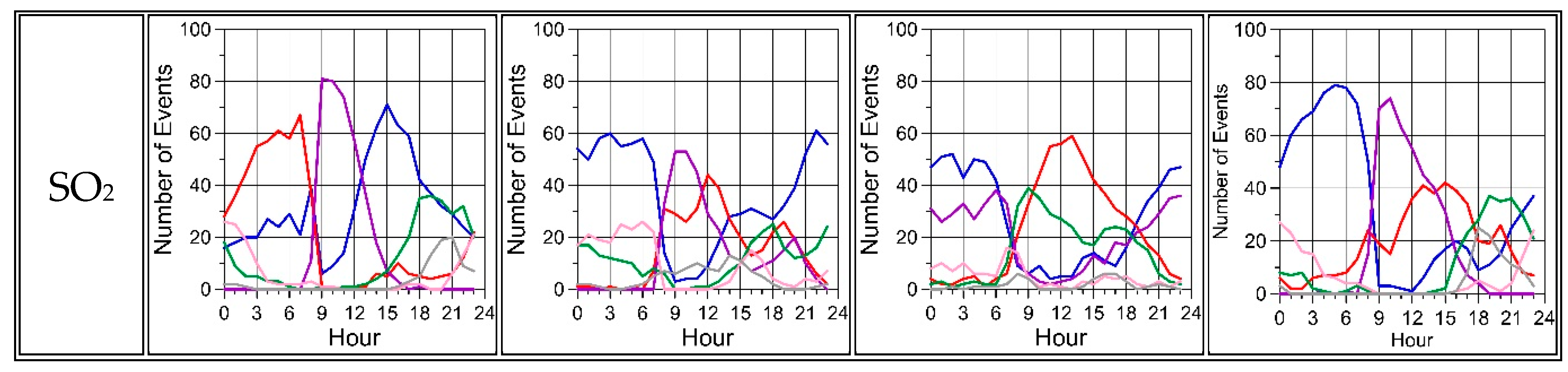
Figure 7 summarizes the application of the k-means clustering method (with k = 6) to the seasonal subsets, Hwinter, Hspring, Hsummer, and Hautumn, of the data objects (events) of wind circulation and pollutant-flows. This figure shows an arrangement with four columns (one per seasonal period) and five rows (one for wind circulation, and four for the pollutant-flows of NO2, O3, PM10, and SO2). Each graph shows six plots (one per cluster) differentiated by the line color. The algorithm enumerates the clusters according to their sizes, from the larger to the smaller, so colors mean no more. Each plot presents the hourly population of one cluster, that is to say, the number of data objects belonging to the cluster as a function of the hour of the day (Mexico City local time, UTC-6 h).
For wind circulation or any given pollutant-flow, a qualitative comparison of graphs in the respective row allowed recognizing some seasonal similarities and differences between the clusters. For example, for the wind circulation (first row), if we pay attention to the clusters represented by a blue-line plot in the four seasons, we can observe an evident regularity: the hourly populations have similar trends and indicate that the majority of their events occurred during the night, mainly from midnight until dawn. We interpreted this regularity as the possible existence of a wind pattern. The plots of the pollutant-flows also show a similar regularity.
The trends of the hourly populations of the clusters provide useful but insufficient information for discovering patterns in sets of events of wind circulation or pollutant-flows. In [25], the authors detected two wind clusters with similar trends in the hourly populations (both in the number of events and in the times of occurrence), but in one case the winds were blowing from the north and in another one from the south, indicating different patterns of wind circulation. However, we can use the information provided by the values of the 16 parameters of the 4-cell model to complement the pattern identification process.
Eight of the sixteen parameters of the 4-cell model are the components of the flow vectors in the quadrants (NW, NE, SW, and SE) of the MCMA. This complementary information and the hourly population plots allowed recognizing the wind circulation patterns shown in Figure 8, and the pollution-flow patterns shown in Figure 9, Figure 10, Figure 11 and Figure 12. We found seven patterns for wind circulation and nine patterns for each of the pollutant-flows (NO2, O3, PM10, and SO2). In Figure 8, we show the hourly population of each wind pattern and a graphic representation of the wind velocity at the quadrants. Figure 9, Figure 10, Figure 11 and Figure 12 show the hourly population of each pattern, a graphic representation of the flow vector at the quadrants, the surface distribution of the pollutant concentration, and the mean spatial pollutant concentration (expressed in ppb for NO2, O3, and SO2, and in µgm−3 for PM10). In these figures, the hourly population of a pattern is an average over the seasons the pattern occurred; the vectors (the wind velocity and the pollutant-flow vectors) are averages over the elements of the pattern and the seasons; the spatial distribution of the pollutant concentrations is the average over the pattern elements and seasons; and the mean spatial concentration of a pollutant is the average over the positions of the average pollutant distribution. The lengths of the arrows that represent the wind and flow vectors were scaled to get the larger one fitted in the square that represents the quadrant, allowing a qualitative comparison of the vector magnitudes among the patterns of wind circulation or the patterns of any of the pollutant flows.
3.1. Wind Circulation Patterns
The proposed methodology for examining the database of the wind events that occurred in Mexico City from 2001 to 2010 allowed discovering there the presence of seven wind circulation patterns and the estimation of their seasonal and annual occurrence frequencies, which we summarized in Table 2. We denoted these patterns as WIND-Pn, with n = 1, 2,…, 7, and enumerated them trying to follow the order of their appearance during the day. In Figure 8, we presented the hourly population of each wind pattern, including a sketch out of the corresponding wind velocity in the city quadrants.
In the following paragraphs, we provide brief descriptions of the wind circulation patterns. We used the Mexico City local time (UTC-6 h) in all figures and descriptions.
WIND-P1: early morning downslope winds. WIND-P1 was the wind pattern with the highest annual frequency (30%). It was observed systematically throughout the year during the night, showing a large peak around hour 6 (Figure 8) and a small peak around hour 15. The mean wind velocities at the quadrants suggest downslope winds from the surrounding mountains, converging towards Mexico City basin. The converging winds represented by the small peak reflect the presence of convective upwards winds due to the urban heat island (UHI) in the Mexico City region. Jauregui [7] and Klaus et al. [33] pointed out that the Mexico City downslope winds are reinforced by UHI.
WIND-P2: northeasterly and easterly winds. The annual average frequency of this wind pattern was 21%. It is observed systematically throughout the year, especially during winter (25%) and summer (24%). The mean velocities correspond to winds blowing from NE in almost all the quadrants of the city (trade winds). The wind events of this pattern occurred from the sunrise (hour 7) up to the hour 17. Its hourly population presents a high peak between hours 10 and 11.
WIND-P3: midday northerly winds. This pattern had an annual frequency of 9%. It was observed during spring (12%), summer (9%), and autumn (14%) from hour 7 to hour 21, with a peak around hour 13. The mean wind velocities in the quadrants indicate winds blowing from the north and northeast sectors.
WIND-P4: westerly and southerly winds. This wind pattern was observed only winter season with a seasonal frequency of 20%; its events occurred throughout the day, but mainly from noon to midnight, reaching its maximum population around hour 17. The mean wind velocities represent winds with a westerly component in the west quadrants and southerly winds in the east quadrants. These velocities correspond to winds blowing from the south and southeast city sectors through a gap between the mountains of the Sierra Ajusco-Chichinautzin and the Sierra Nevada, following the ventilation channel S–N located at the east side of the city (Figure 1). The local winds of this pattern could be related to the subtropical jet stream of winter [34] or with the westerlies that are permanently occurring in subtropical and middle latitudes, but coupled with the winds driven by the gap between the mountains located at the southeast. Doran and Zhong [35] described the main characteristics of a gap wind system in the southeastern corner of Mexico City that produces low-level jets occurring regularly during the late winter.
WIND-P5: afternoon northerly winds. This pattern was observed throughout the year with an annual frequency of 12%. It occurred from noon to midnight, with its maximum around hour 19. The mean wind velocities at the quadrants indicate winds blowing from the north sectors.
WIND-P6: midnight downslope winds. This pattern was observed systematically throughout the year, mainly during the nighttime hours, from the sunset (hour 18) to the sunrise (hour 6 of the next day), with its maximum around midnight. It got an annual average frequency of 18%. The population plot of this pattern has a small peak close to hour 15, which could be related to the UHI effect of the city. The wind velocities in the western quadrants of the city represent downslope flows from Sierra de las Cruces (at west) and Sierra del Ajusco-Chichinautzin (located at SW and S) toward the town. In the eastern quadrants, otherwise, late afternoon northerly gap winds are observed guided by the S–N ventilation channel of the city.
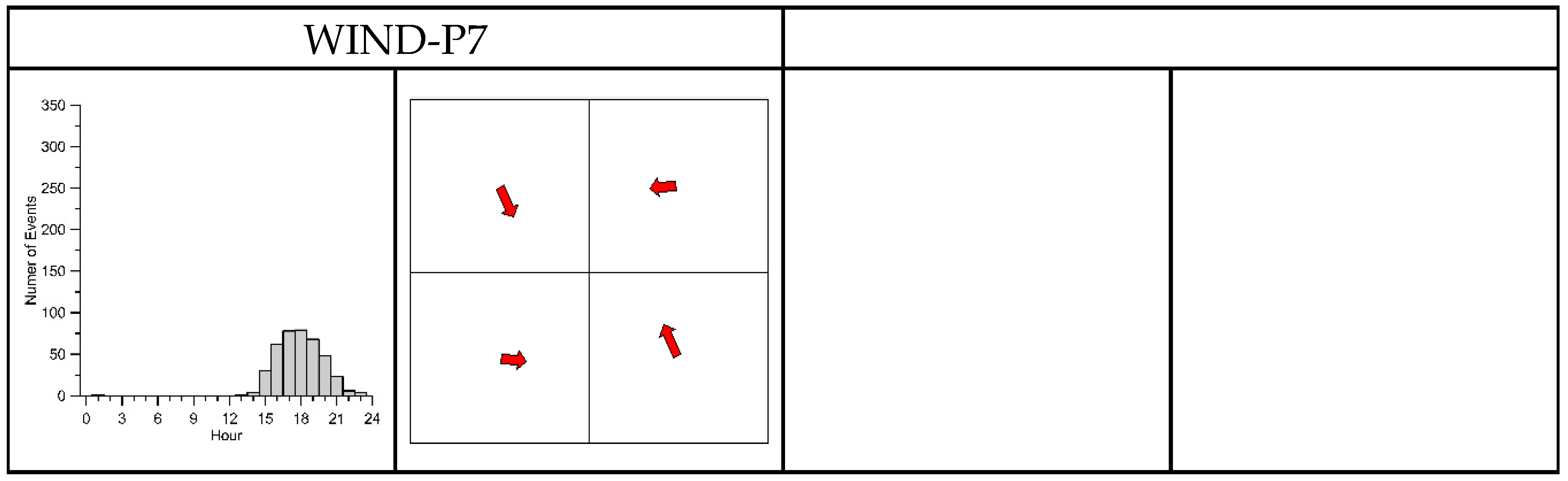
WIND-P7: UHI-driven winds. This wind pattern was observed only during the spring (9%) and autumn (10%) seasons, with a low annual occurrence frequency of 5%. The wind events of this pattern occurred from the hour 14 to the hour 22, and its population reached a maximum value close to the hour 17. The mean wind velocities of the city quadrants indicate cyclonic winds converging towards Mexico City downtown, which seems to be related to an upwards flow driven by the UHI.
Summarizing, the wind patterns with the most significant frequencies were WIND-P1 and WIND-P2, with annual values of 30% and 21%, respectively. These two patterns, however, correspond to small velocities in comparison with the other five wind patterns. An outstanding feature of WIND-P1 is that, although its events occurred mainly during the night with converging winds, it also comprises daylight events of winds with the same characteristic of convergence towards the city downtown. We cannot interpret these last events as katabatic winds produced by the mountain-valley system; instead, we must understand them as winds associated with convective upwards flows driven by the urban heat island (UHI) effect. The pattern WIND-P6 also occurred during the night, but it peaked at midnight. This wind pattern comprises the downslope winds of the first hours of the night and also reflects the effect of the late afternoon northerly gap winds. The patterns WIND-P3 and WIND-P5 reflect the well-known prevailing winds from N and NE of the Mexico City region, and WIND-P2 evidence the occurrence of the trade winds.
The wind patterns with the most significant frequencies were WIND-P1 and WIND-P2, with annual values of 30% and 21%, respectively. These two patterns, however, correspond to small velocities in comparison with the other five wind patterns. An outstanding feature of WIND-P1 is that, although its events occurred mainly during the night with converging winds, it also comprises daylight events of winds with the same characteristic of convergence towards the city downtown. We cannot interpret these last events as katabatic winds produced by the mountain–valley system; instead, we must understand them as winds associated with convective upwards flows driven by the urban heat island (UHI) effect. The pattern WIND-P6 also occurred during the night, but it peaked at midnight. This wind pattern comprises the downslope winds of the first hours of the night and also reflects the effect of the late afternoon northerly gap winds. The patterns WIND-P3 and WIND-P5 reflect the well-known prevailing winds from N and NE of the Mexico City region, and WIND-P2 evidence the occurrence of the trade winds.
Our wind patterns agree quite well with the Mexico City wind patterns obtained in [25] for the period 2001–2006 with a slightly different methodology. In Table 3, we described the correspondence between these two sets of patterns. The first column contains the wind patterns WP1-WP7 reported in [25]; the second column presents the wind patterns obtained in the present work; and, the last column provides a brief description of the main characteristics of these patterns.
The main differences between both sets of patterns were:
- The pattern WIND-P4 includes the wind patterns WP4 (southerly winds) and WP5 (westerly winds) reported in [25]. However, we detected the pattern WIND-P4 only during the winter season, while the pattern WP4 occurred throughout the year (although with tiny frequencies in spring, summer, and autumn), and the pattern WP5 was only observed during the first semester of the year (winter and spring seasons).
- We recognized a pattern (WIND-P7) associated with cyclonic winds strongly converging towards Mexico City downtown during the daylight hours. The winds in this pattern indicate an upwards flow driven by the UHI. No report exists in [25] about a similar pattern.
3.2. Pollutant Flow Patterns
In Table 4, Table 5, Table 6 and Table 7, we enumerated the pollutant-flow patterns (NO2, O3, PM10, and SO2) that we identified for the Mexico City region, their seasonal and annual frequencies and flow intensities (the magnitudes of the flow vectors), and the associated wind circulation patterns. In Figure 9, Figure 10, Figure 11 and Figure 12, for each pollutant-flow pattern, we presented the average population plot, the mean pollutant-flow vectors at the quadrants NW, NE, SW, and SE of the city, the pollutant surface distribution averaged over the pattern, and its mean spatial value. We denoted the pollution-flow patterns as POL-Pn, where POL indicates the pollutant (POL = NO2, O3, PM10, and SO2), and n is a consecutive integer number from 1 to 9. The cells with the value 0.00 in the tables indicate the seasonal periods where some flow patterns were not detected.
In general, although the pollutant concentrations modulate the magnitudes of the flow vectors, the pollutant-flow patterns reflected the directional characteristics inherited from the wind patterns.
3.2.1. The NO2 Flow Patterns
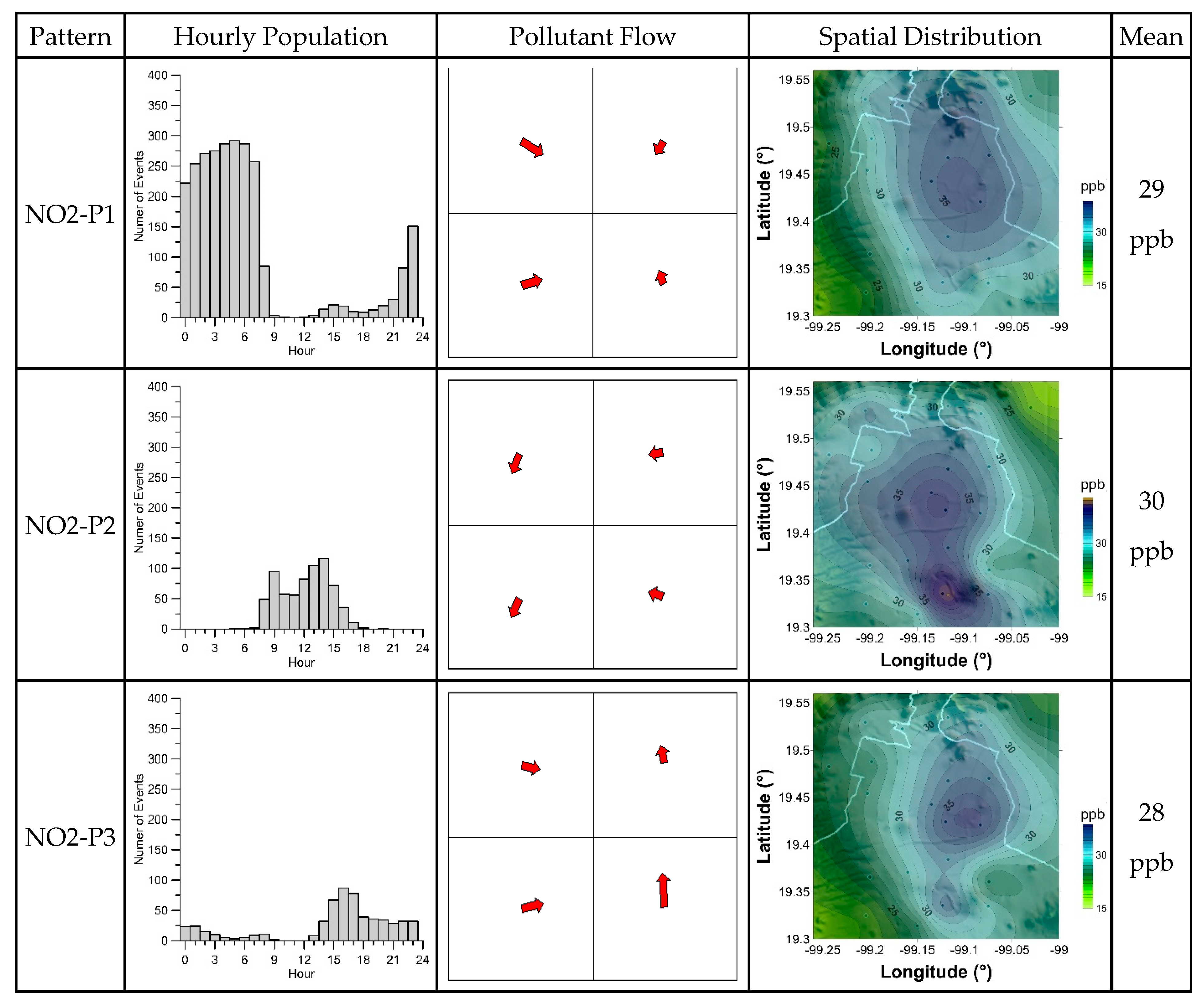
We identified nine NO2 flow patterns for the Mexico City region. Table 4 shows the seasonal and annual average frequencies and average flow intensities of the patterns, expressed in percent (%) and µgm−2s−1, respectively. As shown in Figure 9, these flow patterns closely resemble the wind circulation patterns, and Table 4 summarized the relationship between the pollutant-flow and wind circulation patterns.
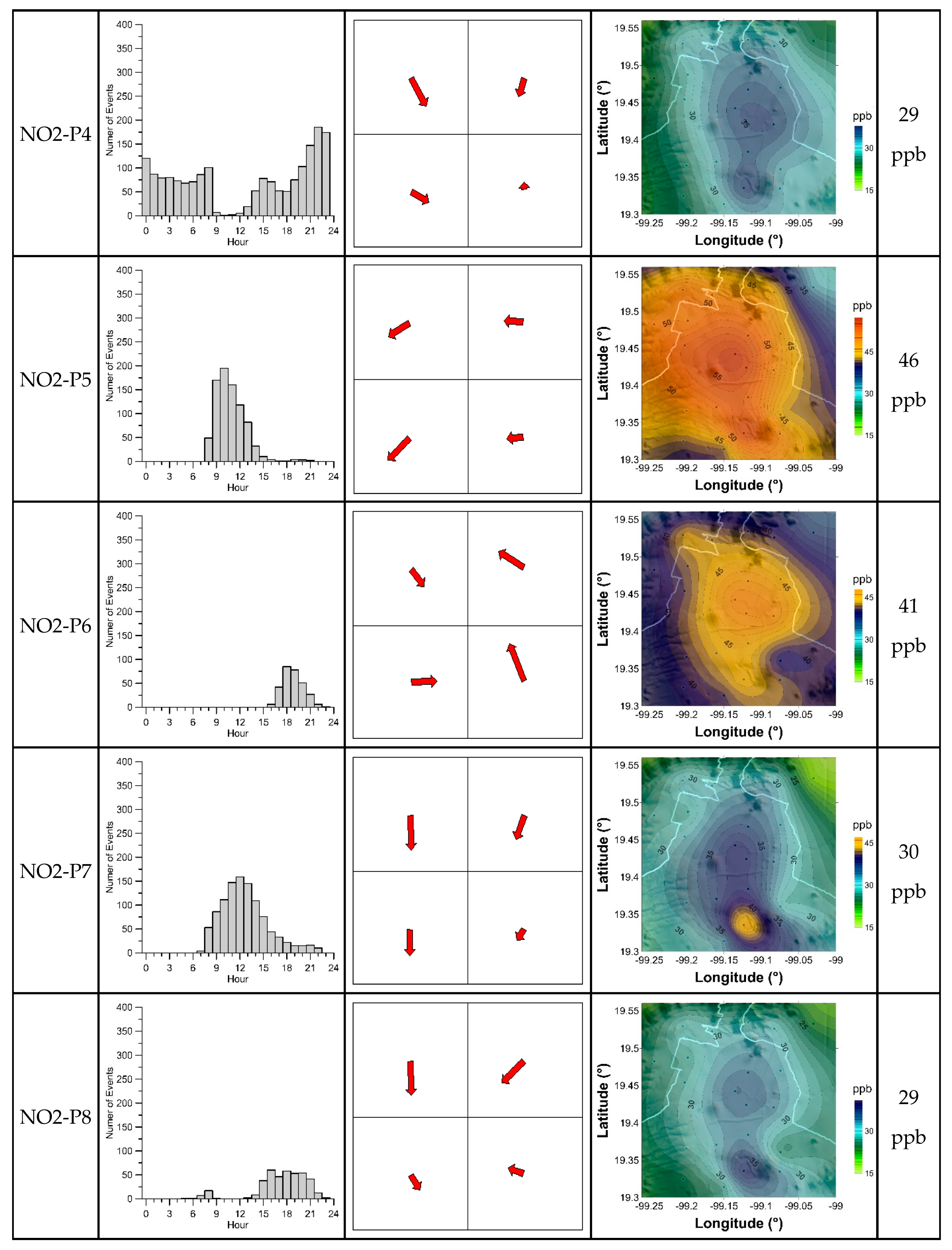
The NO2 flow patterns with the most significant annual frequencies were NO2-P1 (30%), NO2-P4 (20%), and NO2-P7 (12%), but the patterns with the most substantial annual flow intensities were NO2-P5, NO2-P7, and NO2-P9 with 25.4, 25.3, and 24.5 µgm−2s−1, respectively.
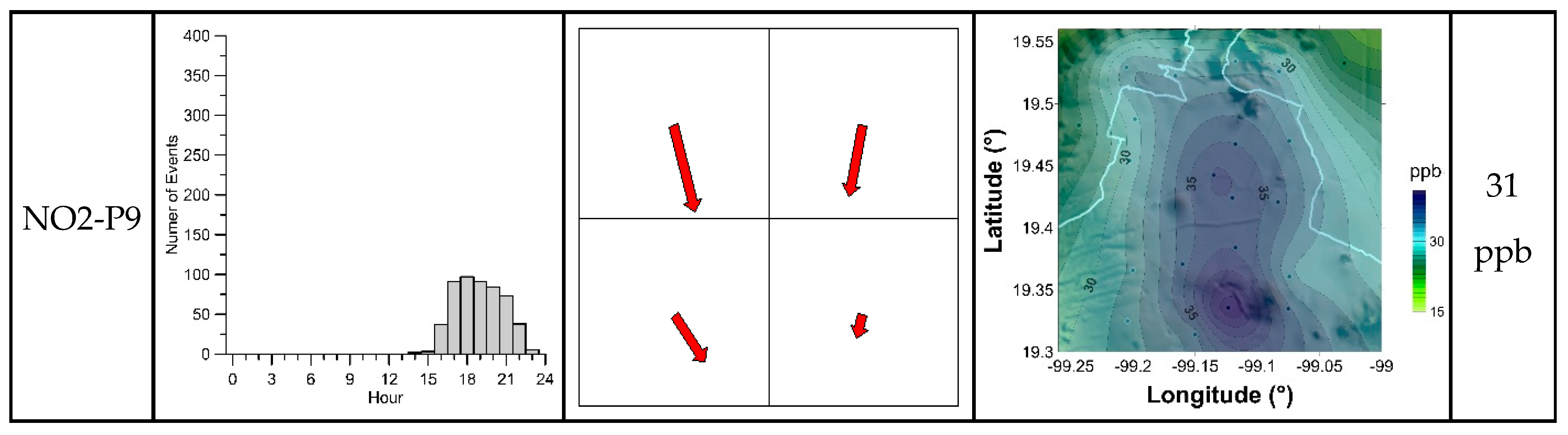
The flow patterns NO2-P4, NO2-P7, NO2-P8, and NO2- P9 carry nitrogen dioxide from the north to the south quadrants of the city, particularly the pattern NO2-P9, although it occurred only during the second semester of the year. The events of these patterns take the ozone precursor to the SW and SE quadrants, contributing actively to the ozone formation in this area throughout the year.
The patterns NO2-P2 and NO2-P5 carry the pollutant from the eastern to the western quadrants of the city following the trade winds. The events of the NO2-P3 and NO2-P6 patterns, differently, take nitrogen dioxide from west to east on the west side of the city, but from south to north on the eastern side. However, while the pattern NO2-P3 reflects a coupling of the westerly winds and the afternoon southerly gap winds, the pattern NO2-P6 reflects cyclonic transport driven by the UHI.
During the night, the events of the pattern NO2-P1, follow the downslope winds from the surrounding mountains and carry NO2 to the city downtown. In comparison with the patterns of other pollutants (O3, PM10, and SO2), the NO2-P1 flow pattern is the only one that revealed considerable nocturnal transport due to the downslope winds. The main reason is that NO2 accumulates during the night since there are no photochemical reactions that consume it, and some of the mobile sources, which are responsible for approximately 86% of nitrogen oxide emissions in the Mexico City region [3], remain active during the night.
The NO2 surface distributions, which are averages over the events of the NO2 flow patterns, reveal a North–South part of the city as the zone with the higher NO2 concentrations. This zone extends around the N–S axis that separates the west from the east quadrants (although slightly shifted to the eastern quadrants). The highest NO2 levels occurred, in general, in the south sector, close to the Huizachtepetl (Cerro de la Estrella).
The surface NO2 distributions with the highest concentrations were in connection with the NO2-P5 and NO2-P6 flow patterns, with mean spatial levels of 46 and 41 ppb. These high levels of NO2 were detected mainly during the winter and autumn. We note that, in these two cases, the high levels of NO2 extended spatially, covering almost completely the city. In the first case, it was a consequence of blocked transport by the mountains of the Sierra las Cruces, while in the second case, the high levels were a consequence of the cyclonic wind convergence driven by the UHI.
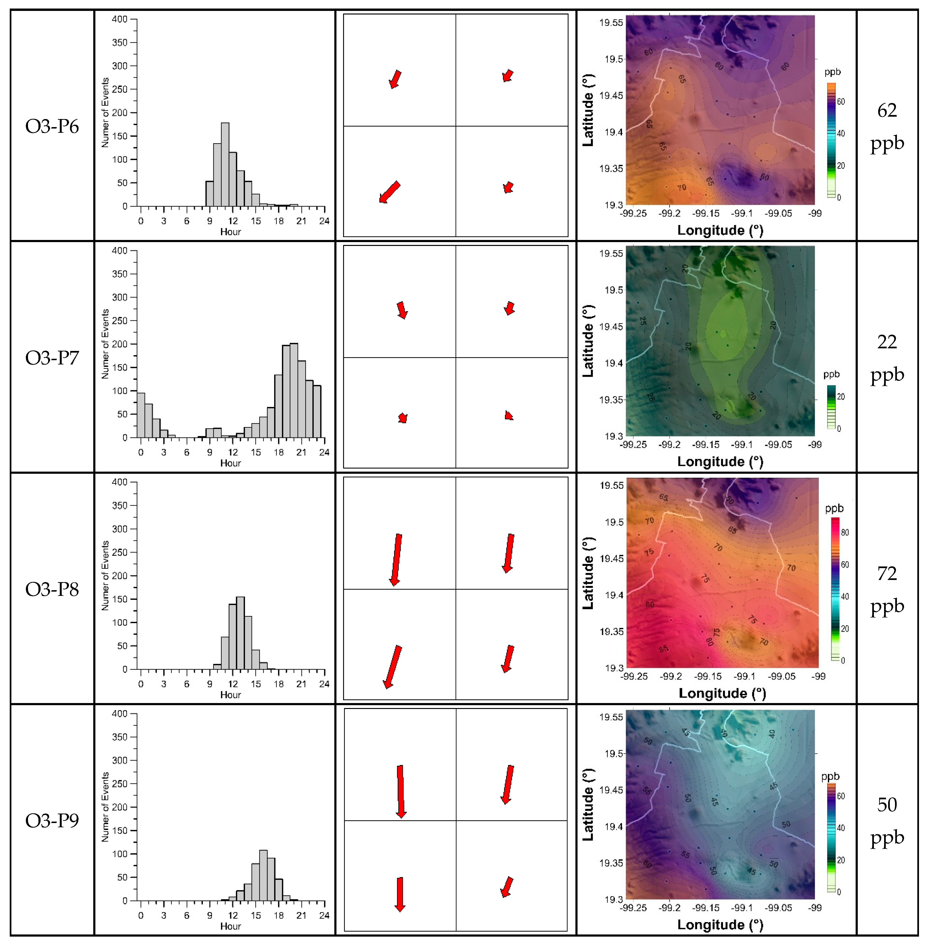
3.2.2. The O3 Flow Patterns
In Table 5 and Figure 10, we summarized the main characteristics of the O3 flow patterns that we identified. In Table 5, we included the average seasonal and annual occurrence frequencies (%) and flow intensities (µg m−2s−1) of the flow patterns, and the wind patterns from which they inherited their circulation characteristics.
The flow vectors of the diurnal flow patterns O3-P6, O3-P8, and O3-P9 have considerable northerly components and convey ozone from the NW and NE to the SW and SE city quadrants, providing substantial contributions to the high ozone concentrations frequently observed in the south sectors (especially in SW) of the city throughout the year.
The flow patterns O3-P6, O3-P8, and O3-P9 revealed the highest flow intensities (43, 82, and 74 µgm−2s−1, on annual average). Seasonally, we observed the highest O3 flow intensities during the spring, summer, and autumn.
The flow patterns O3-P3 and O3-P5 bring ozone from East to West in the city following the trade winds (pattern WIND-P2). These patterns reveal flow vectors from NE in the west quadrants of the city, and because of the mountains barrier (Sierra Las Cruces and Sierra Ajusco Chichinautzin), they contribute to the ozone accumulation at SW sector of the Mexico City region. The O3 surface distributions, averaged over the events of these flow patterns, reveal, in fact, an evident and significant ozone accumulation (ranging from 70 to 100 ppb, approximately) at the SW quadrant.
The flow patterns O3-P1 and O3-P7 comprised nighttime flow events and had the first and second-largest occurrence frequencies. However, their flow intensities are tiny because of the low ozone concentrations (12 ppb and 22 ppb on average, respectively) in the nocturnal atmosphere (ozone production is of photochemical nature). It is interesting to note that the patterns O3-P1 and O3-P7 and the patterns NO2-P1 and NO2-P4 reveal opposite behaviors (during the night, one observes NO2 accumulation while O3 decreases to its lowest levels) due to its relationship through the atmospheric photochemistry.
The O3-P2 is a flow pattern detected during the evening, driven by the UHI winds. It brings ozone from the surrounding parts of the city towards downtown, where an upwards convective flow takes ozone out there again, keeping the ozone levels relatively small in the city.
During winter, the flow events of the O3-P4 pattern bring ozone from west to east in the west side quadrants with small flow intensities, but the same flow pattern carries a considerable amount of ozone from south to north in the east side quadrants of the city, following the ventilation channel located at the west side of Sierra Nevada.
In general, the O3 surface distributions show relative small concentrations where the NO2 surface distributions show large emissions and vice versa. It is an evident behavior because of the NOx-O3 photochemical interactions.
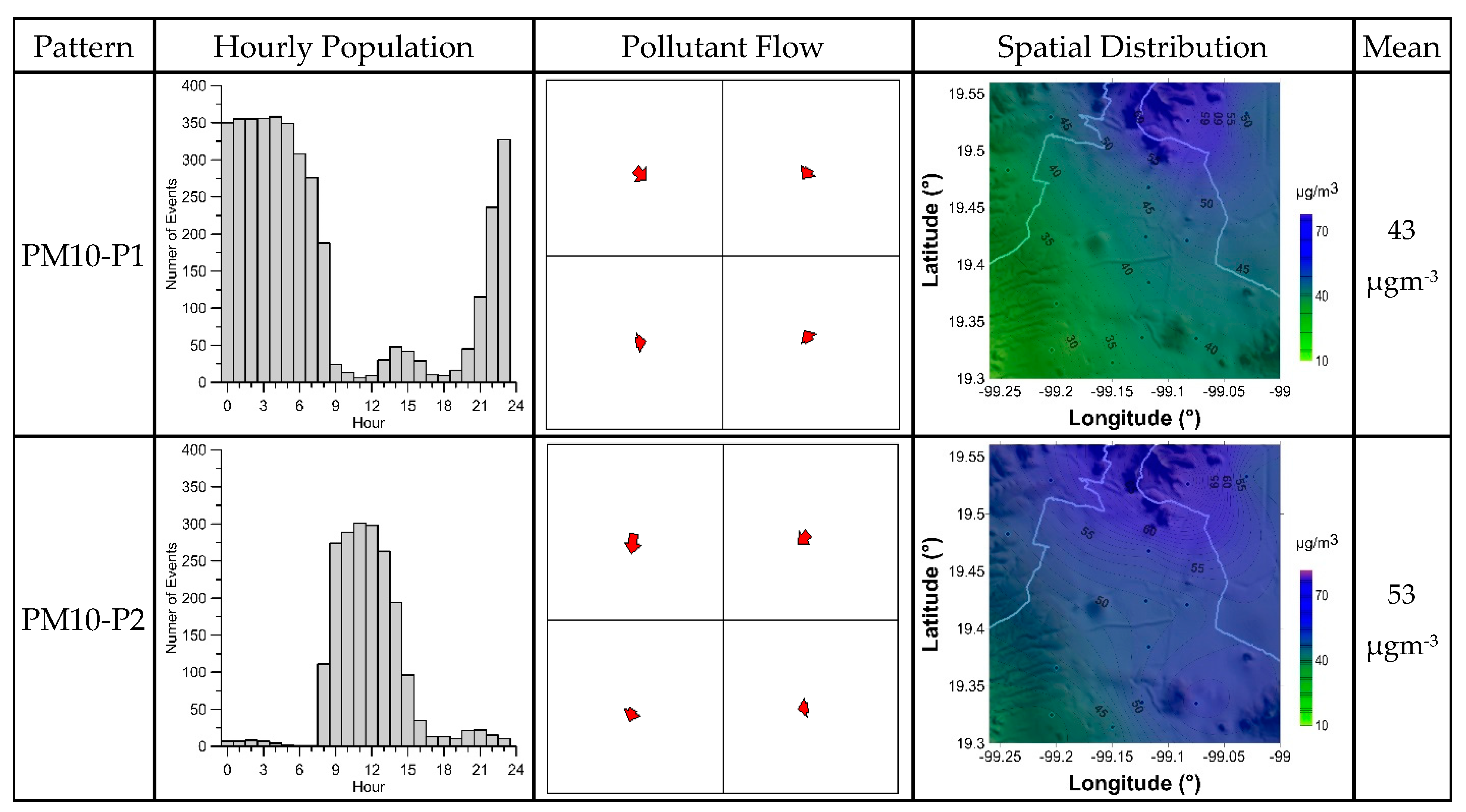
3.2.3. The PM10 Flow Patterns
We recognized nine PM10 flow patterns, which we enumerated in Table 6 and sketched out in Figure 11. In Table 6, we presented the seasonal and annual averages of the occurrence frequencies and the flow intensities of the PM10 flow patterns, expressed in % and µg/m2s, respectively. The directional characteristics of wind inherited by the PM10 patterns are also briefly indicated in this table.
The PM10 flow patterns with the highest annual flow intensities were PM10-P7 (43 µgm−2s−1), PM10-P6 (39 µgm−2s−1), PM10-P5 (35 µgm−2s−1), and PM10-P8 (26 µgm−2s−1); but their annual frequencies were of the smaller (3%, 4%, 2%, and 5%, respectively). All these four patterns reveal a remarkable flow intensity at the NE city quadrant throughout the year, although with different flow directions. The patterns PM10-P6, PM10-P7, and PM10-P8 exhibited also flow vectors with intense northerly components in the NW quadrant, which convey particle PM10 from the north to the south in the west side of the city. The events of these patterns also carried particulate matter from the northeast to the south sectors of the city, particularly in the NE quadrant. The flow intensities of the flow pattern PM10-P6 were 71, 56, and 27 µgm−2s−1 during the winter, spring, and summer seasons; for PM10-P7 were 110 and 63 µgm−2s−1 during the spring and summer, and for PM10-P8 were 43 and 55 µgm−2s−1 during the summer and autumn, respectively.
The events of the PM10-P4 and PM10-P5 flow patterns carried particles from south to northwest in the quadrants of the east side of the city: PM10-P4 with flow intensities of 29 and 27 µgm−2s−1 during the winter and spring, and PM10-P5 with flow intensities of 67 and 71 µgm−2s−1 during the winter and autumn, respectively.
The events of the flow patterns PM10-P1 and PM10-P2 occurred throughout the year with the highest frequencies of occurrence (44% and 22%, on an annual average). The flow intensity of the PM10-P1 (a nocturnal pattern) was too small all year, but the flow intensity of the PM10-P2 (a diurnal pattern) was similar to those of the other flow patterns. The patterns PM10-P1 and PM10-P3 reflect the influence of the downslope winds driven by the mountain-valley system. These patterns, furthermore, reflect the effect of the urban heat island, which is revealed in the hourly population by the small peak around the hour 15 (daylight winds converging to the downtown).
For all the PM10 flow patterns, the average surface distributions of the pollutant reveal the NE quadrant as the zone of the city with the highest PM10 concentrations, and the SW quadrant as the zone with the lowest levels of PM10. It suggests that, at the NE of the town, in the surrounding area of Xalostoc on the east side of the Sierra de Guadalupe, there exists considerable sources of particulate matter, which release PM10 to the atmosphere all year long.
It is interesting to observe that the events of the pattern PM10-P5 revealed flow vectors at the NE and SE quadrants with intense southerly components, which produced, on average, the highest mean spatial concentration of PM10 (81 µgm−3) in the city. This result displays the east side quadrants of the city as the most polluted areas by PM10 during the winter and autumn.
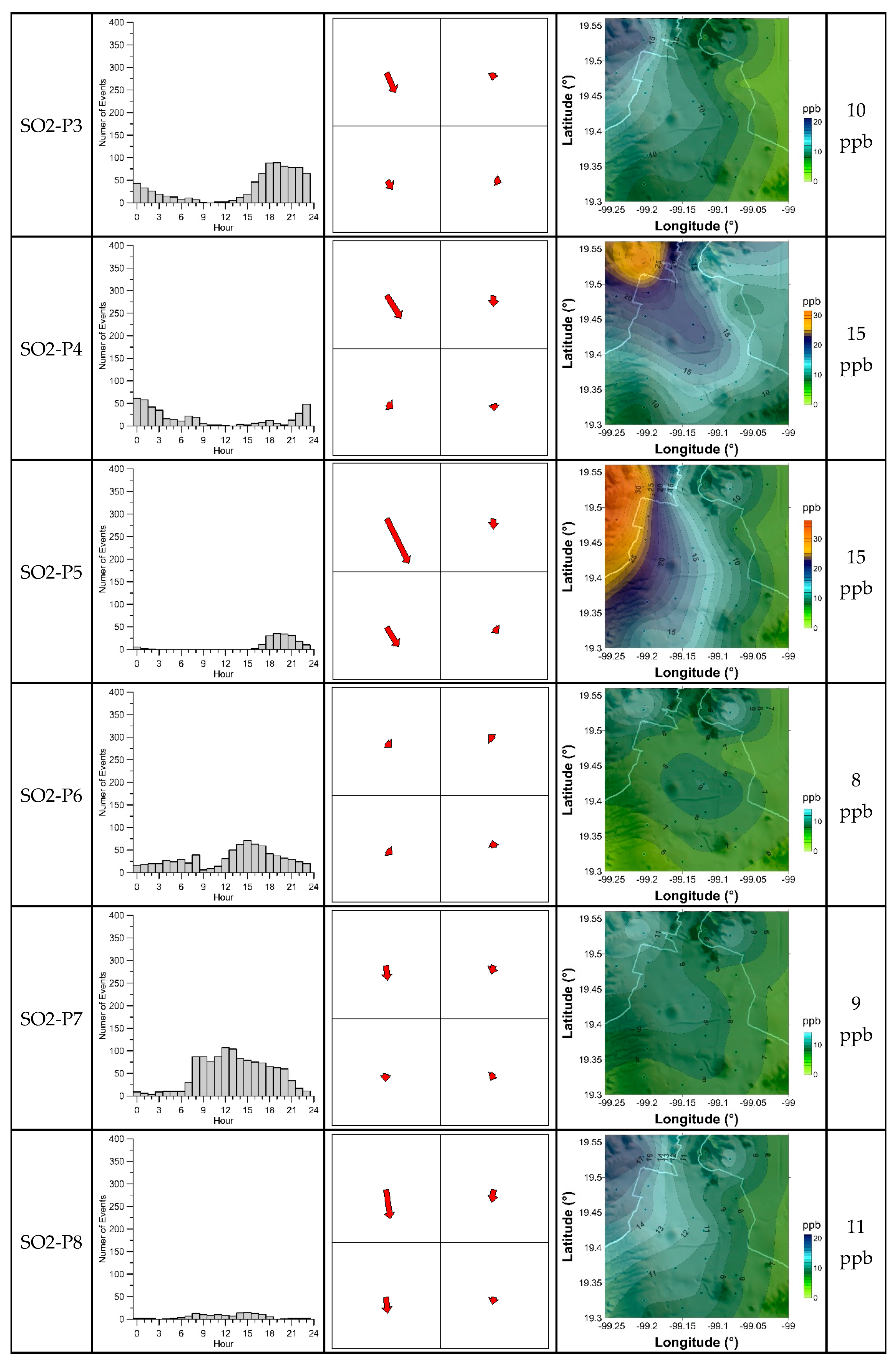
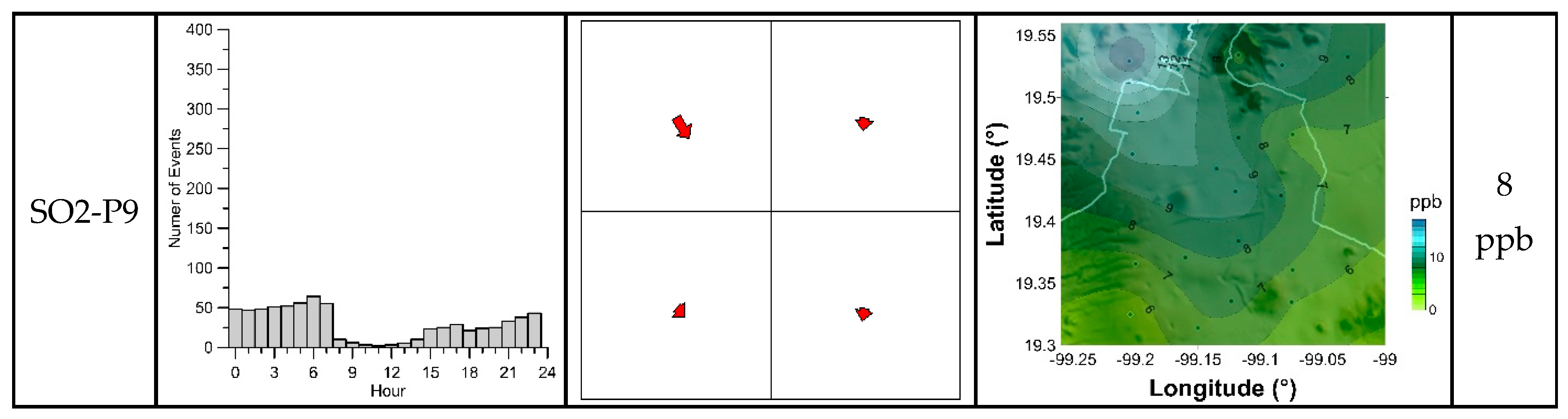
3.2.4. The SO2 Flow Patterns
Table 7 and Figure 12 enumerate and sketch out the SO2 flow patterns that we identified. Table 7 presents the average seasonal and annual occurrence frequencies and flow intensities of these patterns, including their relationship with the wind circulation patterns. Figure 12 shows the hourly population of the patterns, the corresponding flow vectors, and the surface distribution of the SO2 emissions produced by the events of these flow patterns.
We observed, in general, that all the SO2 flow patterns presented small flow intensities and produced small surface concentrations (we underline that the Mexican air quality standard for SO2 is 110 ppb on a 24 h average, and 25 ppb on an annual average). Nevertheless, it is particularly interesting to observe that the flow patterns SO2-P3 (winter, spring, and autumn), SO2-P4 (winter, summer, and autumn), SO2-P5 (winter and autumn), and SO2-P9 (spring and summer), which were detected mainly during the night hours, exhibit the flow vector at the NW quadrant with a flow intensity relatively larger than in the other quadrants. However, the corresponding wind patterns show winds of similar magnitudes in all the quadrants.
The events of the flow patterns SO2-P7 (spring, summer, and autumn) and SO2-P8 (spring and summer) occurred during daylight hours and show the NW-quadrant flow vector larger than in the other quadrants. Consistently with these observations, the mean spatial SO2 surface distributions reveal the NW quadrant of the city as the zone with the highest levels of concentration, particularly in the case of the patterns SO2-P4 and SO2-P5. This situation seems to indicate that in the NW quadrant of the city, there are intense activities that release sulfur dioxide to the atmosphere during the night.
The SO2-P1 and SO2-P2 flow patterns, as was the case with the other pollutants, were the most frequent patterns (33% and 19%, respectively, on annual average) and the only ones detected all over the year; however, their flow intensities were tiny.
4. Conclusions
We used a simple model to define the pollutant-flow conditions in terms of the horizontal components of the flow vector and its gradients (divergence and curl). We applied this model to the hourly data of wind and pollutant concentration measured during the period 2001–2010 by the atmospheric monitoring network of Mexico City. We obtained the main flow patterns of NO2, O3, PM10, and SO2 using a 4-cell model of the city and the k-means algorithm of cluster analysis. Estimations of the seasonal and annual occurrence frequencies and flow intensities of the flow patterns were obtained.
The pollution flow patterns reflect some of the wind circulation conditions of the Mexico City wind patterns; however, since the pollutant-flow conditions also depend on the pollutant concentration, the flow patterns revealed situations of pollutant transport that cannot be inferred simply from the wind circulation modes. Different pollutants under the same wind patterns produced different pollutant-flow patterns. For example, the SO2 flow patterns (SO2-P3, SO2-P4, and SO2-P5) display large flow intensities at the NW quadrant bringing this pollutant towards the Mexico City region, mainly during winter and autumn seasons; however, the corresponding wind patterns exhibit wind velocities with similar magnitudes in almost all the quadrants. The events of the flow patterns SO2-P8 occurred with similar conditions, but during the spring and summer periods. Similarly, the PM10-P4 and PM10-P5, and PM10-P6 and PM10-P7 flow patterns revealed large flow intensities in the NE quadrant, although winds have similar magnitudes in other quadrants.
The pollutant-flow patterns of NO2, O3, PM10, and SO2 represent the main scenarios of the pollutant transport in the Mexico City region. They provide information that can guide, enrich, and enlighten the results of Mexico City air quality studies based on modeling techniques.
Author Contributions
Conceptualization, A.S.; Formal analysis, A.S.; Investigation, S.C.-S. and A.-T.C.-M.; Methodology, A.S., S.C.-S. and A.-T.C.-M.; Software, A.S. and S.C.-S.; Supervision, A.S.; Writing—original draft, A.S., S.C.-S. and A.-T.C.-M.; Writing—review & editing, A.S. and A.-T.C.-M.
Funding
This research received no external funding.
Acknowledgments
We thank Ana Laura Colín Aguilar (Instituto Nacional de Electricidad y Energías Limpias) for beneficial comments to make the paper more comprehensible.
Conflicts of Interest
The authors declare no conflict of interest.
References
- Pascal, M.; Corso, M.; Chanel, O.; Declercq, C.; Badaloni, C.; Cesaroni, G.; Henschel, S.; Meister, K.; Haluza, D.; Martin-Olmedo, P.; et al. Assessing the public health impacts of urban air pollution in 25 European cities: Results of the Aphekom project. Sci. Total Environ. 2013, 449, 390–400. [Google Scholar] [CrossRef] [PubMed]
- Sicard, P.; Lesne, O.; Alexandre, N.; Mangin, A.; Collomp, R. Air quality trends and potential health effects —Development of an aggregate risk index. Atmos. Environ. 2011, 45, 1145–1153. [Google Scholar] [CrossRef]
- Secretaría del Medio Ambiente. Gobierno del Distrito Federal. Inventario de Emisiones de Contaminantes Criterio de la Zona Metropolitana del Valle de México, 1st ed.; Secretaría del Medio Ambiente del DF: Mexico City, Mexico, 2008. [Google Scholar]
- Bravo, H.A.; Torres, R.J. Air Pollution Levels and Trends in the Mexico City Metropolitan Area. In Urban Air Pollution and Forests: Resources at Risk in the Mexico City Air Basin; Springer: New York, NY, USA, 2002; pp. 121–159. [Google Scholar]
- Bonner, J.C.; Rice, A.B.; Lindroos, P.M.; O’Brien, P.O.; Dreher, K.L.; Rosas, I.; Alfaro-Moreno, E.; Osornio-Vargas, A.R. Induction of the lung myofibroblast PDGF receptor system by urban ambient particles from Mexico City. Am. J. Respir. Cell. Mol. Biol. 1998, 19, 672–680. [Google Scholar] [CrossRef]
- Osornio-Vargas, A.R.; Bonner, J.C.; Alfaro-Moreno, E.; Martinez, L.; Garcia-Cuellar, C.; Ponce-de-Leon-Rosales, S.; Miranda, J.; Rosas, I. Proinflammatory and cytotoxic effects of Mexico City air pollution particulate matter in vitro are dependent on particle size and composition. Environ. Health Perspect. 2003, 111, 1289–1293. [Google Scholar] [CrossRef]
- Jáuregui, E. Local wind and air pollution interaction in the Mexico basin. Atmósfera 1988, 1, 131–140. [Google Scholar]
- De Foy, B.; Caetano, E.; Magaña, V.; Zitácuaro, A.; Cárdenas, B.; Retama, A.; Ramos, R.; Molina, L.T.; Molina, M.J. Mexico City basin wind circulation during the MCMA-2003 field campaign. Atmos. Chem. Phys. 2005, 5, 2267–2288. [Google Scholar] [CrossRef] [Green Version]
- Oke, T.R.; Zeuner, G.; Jauregui, E. The Surface Energy Balance in Mexico City. Atmos. Environ. Part B Urban Atmos. 1992, 26, 433–444. [Google Scholar] [CrossRef]
- Jauregui, E.; Luyando, E. Global radiation attenuation by air pollution and its effects on the thermal climate in Mexico City. Int. J. Clim. 1999, 19, 683–694. [Google Scholar] [CrossRef]
- Salcido, A.; Celada, A.T.; Villegas, R.; Salas, H.; Sozzi, R.; Georgiadis, T. A micrometeorological database for the Mexico City Metropolitan Area. Nuovo Cim. C Geophys. Space Phys. C 2003, 26, 317–355. [Google Scholar]
- Castro, T.; Salcido, A. Influencia de la contaminación atmosférica de la Zona Metropolitana de la Ciudad de México en tres sitios perimetrales. In Contaminación Atmosférica V; El Colegio Nacional: Mexico City, Mexico, 2006. [Google Scholar]
- Molina, L.T.; Madronich, S.; Gaffney, J.S.; Apel, E.; de Foy, B.; Fast, J.; Ferrare, R.; Herndon, S.; Jimenez, J.L.; Lamb, B.; et al. An overview of the MILAGRO 2006 Campaign: Mexico City emissions and their transport and transformation. Atmos. Chem. Phys. 2010, 10, 8697–8760. [Google Scholar] [CrossRef] [Green Version]
- Bossert, J.E. An Investigation of Flow Regimes Affecting the Mexico City Region. J. Appl. Meteorol. 1997, 36, 119–140. [Google Scholar] [CrossRef] [Green Version]
- Fast, J.D.; Zhong, S. Meteorological factors associated with inhomogeneous ozone concentrations within the Mexico City basin. J. Geophys. Res. 1998, 103, 18927–18946. [Google Scholar] [CrossRef]
- Doran, J.C.; Abbott, S.; Archuleta, J.; Bian, X.; Chow, J.; Coulter, R.L.; de Wekker, S.F.J.; Edgerton, S.; Elliott, S.; Fernandez, A.; et al. The IMADA-AVER Boundary Layer Experiment in the Mexico City Area. Bull. Am. Meteorol. Soc. 1998, 79, 2497–2508. [Google Scholar] [CrossRef]
- Mora, M.; Braun, R.A.; Shingler, T.; Sorooshian, A. Analysis of remotely sensed and surface data of aerosols and meteorology for the Mexico Megalopolis Area between 2003 and 2015. J. Geophys. Res. Atmos. JGR 2017, 122, 8705–8723. [Google Scholar] [CrossRef] [PubMed] [Green Version]
- Fast, J.D.; de Foy, B.; Acevedo Rosas, F.; Caetano, E.; Carmichael, G.; Emmons, L.; McKenna, D.; Mena, M.; Skamarock, W.; Tie, X.; et al. A meteorological overview of the MILAGRO field campaigns. Atmos. Chem. Phys. 2007, 7, 2233–2257. [Google Scholar] [CrossRef] [Green Version]
- Salcido, A.; Celada-Murillo, A.T.; Castro, T. A meso-β Scale Description of Surface Wind Events in Mexico City during the MILAGRO 2006 Campaign. In Proceedings of the IASTED Technology Conferences, Environmental Management and Engineering (EME), Banff, AB, Canada, 15–17 July 2010; Alhajj, R.S., Leung, V.C.M., Petela, R., Saif, M., Thring, R., Eds.; Acta Press: Calgary, AB, Canada, 2010. Track 699-041. [Google Scholar] [CrossRef]
- Celada-Murillo, A.; Carreón-Sierra, S.; Salcido, A.; Castro, T.; Peralta, O.; Georgiadis, T. Main Characteristics of Mexico City Local Wind Events during the MILAGRO 2006 Campaign within a Meso-β Scale Lattice Wind Modeling Approach. ISRN Meteorol. 2013, 2013, 605210. [Google Scholar] [CrossRef]
- Salcido, A.; Carreón-Sierra, S.; Celada-Murillo, A.T. A Brief Clustering Analysis of the Mexico City Local Wind States Occurred During the MILAGRO Campaign. In Proceedings of the IASTED International Conference on Environmental Management and Engineering (EME), Banff, AB, Canada, 16–17 July 2014. [Google Scholar] [CrossRef]
- Klaus, D.; Poth, A.; Voss, M.; Jauregui, E. Ozone distributions in Mexico City using principal component analysis and its relation to meteorological parameters. Atmósfera 2001, 14, 171–188. [Google Scholar]
- De Foy, B.; Fast, J.D.; Paech, S.J.; Phillips, D.; Walters, J.T.; Coulter, R.L.; Martin, T.J.; Pekour, M.S.; Shaw, W.J.; Kastendeuch, P.P.; et al. Basin-scale wind transport during the MILAGRO field campaign and comparison to climatology using cluster analysis. Atmos. Chem. Phys. 2008, 8, 1209–1224. [Google Scholar] [CrossRef] [Green Version]
- Salcido, A.; Carreón-Sierra, S.; Georgiadis, T.; Celada-Murillo, A.T.; Castro, T. Lattice Wind Description and Characterization of Mexico City Local Wind Events. Period 2001–2006. Climate 2015, 3, 542–562. [Google Scholar] [CrossRef]
- Carreón-Sierra, S.; Salcido, A.; Castro, T.; Celada-Murillo, A.T. Cluster Analysis of the Wind Events and Seasonal Wind Circulation Patterns in the Mexico City Region. Atmosphere 2015, 6, 1006–1031. [Google Scholar] [CrossRef] [Green Version]
- Mexico City Air Quality Monitoring Network (Sistema de Monitoreo Atmosférico de la Ciudad de México). Available online: http://www.aire.cdmx.gob.mx/default.php (accessed on 23 July 2019).
- Everitt, B.S.; Landau, S.; Leese, M. Cluster Analysis, 4th ed.; Arnold: London, UK, 2001; ISBN 9780340761199. [Google Scholar]
- Hartigan, J.A.; Wong, M.A. Algorithm AS 136: A K-Means Clustering Algorithm. Appl. Stat. 1979, 28, 100–108. [Google Scholar] [CrossRef]
- James, G.; Witten, D.; Hastie, T.; Tibshirani, R. An Introduction to Statistical Learning with Applications in R; Springer: New York, NY, USA; Heidelberg, Germany; Dordrecht, The Netherlands; London, UK, 2013; Corrected at Eighth Printing 2017. [Google Scholar] [CrossRef]
- Shaefer, J.T.; Doswell, C.A. On the interpolation of a vector field. Mon. Weather Rev. 1979, 107, 458–476. [Google Scholar] [CrossRef]
- Salcido, A. A Phenomenological Gradient Approach to Generalized Constitutive Equations for Isotropic Fluids. J. Appl. Math. Phys. 2018, 6, 1494–1506. [Google Scholar] [CrossRef]
- Lohninger, H. DataLab 3.911; Epina GmbH: Gütersloh, Germany, 2019. [Google Scholar]
- Klaus, D.; Jauregui, E.; Poth, A.; Stein, G.; Voss, M. Regular circulation structures in the tropical basin of Mexico City as a consequence of the urban heat island effect. Erdkunde 1999, 53, 231–243. [Google Scholar] [CrossRef]
- Krishnamurti, T.N. The Subtropical Jet Stream of Winter. J. Meterol. 1960, 18, 172–191. [Google Scholar] [CrossRef]
- Doran, J.C.; Zhong, S. Thermally Driven Gap Winds into the Mexico City Basin. J. Appl. Meteorol. 2000, 39, 1330–1340. [Google Scholar] [CrossRef]
Figure 1.
Complex topography in the Mexico City region.

Figure 2.
Study domain for Mexico City and spatial distribution of the stations (white dots) of the wind-monitoring network (REDMET) of the atmospheric monitoring network of Mexico City (SIMAT). The REDMET provides 1-hour average values of wind speed and wind direction, and other properties such as temperature and relative humidity.

Figure 3.
Spatial distribution of the stations (white dots) of the NO2, O3, PM10, and SO2 monitoring networks (RAMA) of SIMAT. The RAMA provides 1-hour average values of the surface concentrations of NO2, O3, PM10, and SO2, among other chemical compounds.
Figure 3.
Spatial distribution of the stations (white dots) of the NO2, O3, PM10, and SO2 monitoring networks (RAMA) of SIMAT. The RAMA provides 1-hour average values of the surface concentrations of NO2, O3, PM10, and SO2, among other chemical compounds.

Figure 4.
Arrangement of the calculation grid nodes Grs and the lattice cells Cij. The green crosses represent the grid nodes, and the red crosses indicate the centers of the lattice cells. In gray, we show the cell Cij.
Figure 4.
Arrangement of the calculation grid nodes Grs and the lattice cells Cij. The green crosses represent the grid nodes, and the red crosses indicate the centers of the lattice cells. In gray, we show the cell Cij.

Figure 5.
Average diurnal behavior of solar radiation (red line), temperature (green line), and wind speed (blue line) in an urban site (Xochimilco) of Mexico City during 2001 [11,25]. We observe that the meteorological events comprised in the six intervals of 0–4, 4–8, 8–12, 12–16, 16–20, and 20–24 h are different from one period to another. This appraisal suggests searching for six clusters during the cluster analysis of the wind and pollutant-flow events.

Figure 6.
Percentage reduction (δ) of the total within-cluster sum of squares, relative to its previous value, as a function of the number of clusters. Here, for the clustering of the winter wind data objects, we observe that from 6 clusters on, the reduction δ is less than 10% each unit step in the increase of the number of clusters: .

Figure 7.
Application of the k-means algorithm (with k = 6) to the seasonal subsets of the data objects of the wind circulation (first row) and pollutant-flows (next four rows) events. Each graph shows six plots, one per cluster, individualized by the color. Each plot expresses the hourly population of the cluster, i.e., the number of data objects (or events) of the cluster as a function of the hour of the day.


Figure 8.
Wind circulation patterns in the Mexico City region during the period 2001–2010. For each pattern, we presented the hourly population (left) and the mean wind velocity (relative to the pattern) at the city quadrants (right). The size of red arrows that stand in for the velocity vectors indicates the velocity magnitude in a scale relative to the edge size of the squares that represent the quadrants.


Figure 9.
Flow patterns of nitrogen dioxide in the Mexico City region during the period 2001–2010. For each pattern, we included the hourly population (second column), the mean flow vectors (relative to the pattern) at the city quadrants (third column), the surface concentration distributions (fourth column) averaged over the events of the flow pattern, and the mean spatial concentration (last column). The size of red arrows that stand in for the NO2 flow vectors indicates the flow intensity in a scale relative to the edge size of the squares that represent the quadrants.


Figure 10.
Flow patterns of ozone in the Mexico City region during the period 2001–2010. For each flow pattern, the figures show the hourly population (second column), the mean flow vectors (relative to the pattern) at the city quadrants (third column), the surface concentration distributions (fourth column) averaged over the events of the flow pattern, and the mean spatial concentration (last column). The size of red arrows that stand in for the O3 flow vectors indicates the flow intensity in a scale relative to the edge size of the squares that represent the quadrants.


Figure 11.
Flow patterns of PM10 in the Mexico City region during the period 2001–2010. For each flow pattern, the figures show the hourly population (second column), the mean flow vectors (relative to the pattern) at the city quadrants (third column), the surface concentration distributions (fourth column) averaged over the events of the flow pattern, and the mean spatial concentration (last column). The size of red arrows that stand in for the PM10 flow vectors indicates the flow intensity in a scale relative to the edge size of the squares that represent the quadrants.


Figure 12.
Flow patterns of sulfur dioxide in the Mexico City region during the period 2001–2010. For each flow pattern, the figures show the hourly population (second column), the mean flow vectors (relative to the pattern) at the city quadrants (third column), the surface concentration distributions (fourth column) averaged over the events of the flow pattern, and the mean spatial concentration (last column). The size of red arrows that stand in for the SO2 flow vectors indicates the flow intensity in a scale relative to the edge size of the squares that represent the quadrants.


Table 1.
Structure of the data matrix for the cluster analysis.
| Columns | Variables |
|---|---|
| 1 | DateTime (MMDDHH) |
| 2–5 | The four values of the 1-cell model parameters: |
| 6–21 | The 16 values of the 4-cell model parameters: |
Table 2.
Seasonal and annual frequencies of the wind circulation patterns (%).
| Pattern | Jan–Mar (Winter) | Apr–Jun (Spring) | Jul–Sep (Summer) | Oct–Dec (Autumn) | Annual |
|---|---|---|---|---|---|
| WIND-P1 | 33 | 31 | 25 | 32 | 30 |
| WIND-P2 | 25 | 18 | 24 | 16 | 21 |
| WIND-P3 | 0 | 12 | 9 | 14 | 9 |
| WIND-P4 | 20 | 0 | 0 | 0 | 5 |
| WIND-P5 | 9 | 9 | 20 | 11 | 12 |
| WIND-P6 | 14 | 21 | 22 | 17 | 18 |
| WIND-P7 | 0 | 9 | 0 | 10 | 5 |
Table 3.
Comparison against the wind patterns reported by Carreón-Sierra et al. [25].
Table 3.
Comparison against the wind patterns reported by Carreón-Sierra et al. [25].
| Carreón-Sierra et al. | This Work | Description |
|---|---|---|
| WP1 | WIND-P1 | Early morning downslope winds |
| WP2 | WIND-P2 | Northeasterly and easterly winds |
| WP3 | WIND-P3 | Midday northerly winds |
| WP4 | WIND-P4 | Westerly winds at the western quadrants and |
| WP5 | Southerly winds at the eastern quadrants | |
| WP6 | WIND-P5 | Afternoon northerly winds |
| WP7 | WIND-P6 | Midnight downslope winds |
| ----- | WIND-P7 | UHI-driven winds |
Table 4.
Frequencies (%) and flow intensities (µg/m2s) of Mexico City NO2 flow patterns (2001–2010).
Table 4.
Frequencies (%) and flow intensities (µg/m2s) of Mexico City NO2 flow patterns (2001–2010).
| Pattern | Wind Pattern Inherited | JAN–MAR (Winter) | APR–JUN (Spring) | JUL–SEP (Summer) | OCT–DEC (Autumn) | ANNUAL | |||||
|---|---|---|---|---|---|---|---|---|---|---|---|
| Freq | Flow | Freq | Flow | Freq | Flow | Freq | Flow | Freq | Flow | ||
| NO2-P1 | WIND-P1 | 37.36 | 10.41 | 23.81 | 7.46 | 35.96 | 10.31 | 22.13 | 13.49 | 29.79 | 10.42 |
| NO2-P2 | WIND-P2 | 18.61 | 15.59 | 0.00 | 0.00 | 12.86 | 16.83 | 0.00 | 0.00 | 7.83 | 8.11 |
| NO2-P3 | WIND-P4 | 15.93 | 18.59 | 10.85 | 16.92 | 0.00 | 0.00 | 0.00 | 0.00 | 6.63 | 8.88 |
| NO2-P4 | WIND-P6 | 11.02 | 32.38 | 24.08 | 19.03 | 17.35 | 27.07 | 29.02 | 7.92 | 20.41 | 21.60 |
| NO2-P5 | WIND-P2 | 10.42 | 46.27 | 17.03 | 24.57 | 0.00 | 0.00 | 10.61 | 30.61 | 9.49 | 25.36 |
| NO2-P6 | WIND-P7 | 6.67 | 21.82 | 0.00 | 0.00 | 0.00 | 0.00 | 6.89 | 5.96 | 3.38 | 6.95 |
| NO2-P7 | WIND-P3 | 0.00 | 0.00 | 14.93 | 42.51 | 15.94 | 28.30 | 16.64 | 30.18 | 11.93 | 25.25 |
| NO2-P8 | WIND-P5 | 0.00 | 0.00 | 9.29 | 26.70 | 8.97 | 24.39 | 0.00 | 0.00 | 4.58 | 12.77 |
| NO2-P9 | WIND-P5 | 0.00 | 0.00 | 0.00 | 0.00 | 8.92 | 49.99 | 14.69 | 48.00 | 5.95 | 24.50 |
Table 5.
Frequencies (%) and flow intensities (µg/m2s) of the Mexico City O3 flow patterns (2001–2010).
Table 5.
Frequencies (%) and flow intensities (µg/m2s) of the Mexico City O3 flow patterns (2001–2010).
| Pattern | Wind Pattern Inherited | JAN–MAR (Winter) | APR–JUN (Spring) | JUL–SEP (Summer) | OCT–DEC (Autumn) | ANNUAL | |||||
|---|---|---|---|---|---|---|---|---|---|---|---|
| Freq | Flow | Freq | Flow | Freq | Flow | Freq | Flow | Freq | Flow | ||
| O3-P1 | WIND-P1 | 54.54 | 6.47 | 46.57 | 6.66 | 41.35 | 7.89 | 52.20 | 4.41 | 48.64 | 6.36 |
| O3-P2 | WIND-P7 | 11.53 | 5.00 | 7.74 | 4.22 | 0.00 | 0.00 | 6.21 | 8.92 | 6.34 | 4.54 |
| O3-P3 | WIND-P2 | 11.48 | 13.84 | 0.00 | 0.00 | 0.00 | 0.00 | 10.79 | 29.21 | 5.55 | 10.76 |
| O3-P4 | WIND-P4 | 8.29 | 46.08 | 0.00 | 0.00 | 0.00 | 0.00 | 0.00 | 0.00 | 2.04 | 11.52 |
| O3-P5 | WIND-P2 | 7.50 | 43.99 | 0.00 | 0.00 | 6.52 | 53.26 | 0.00 | 0.00 | 3.49 | 24.31 |
| O3-P6 | WIND-P2 | 6.67 | 61.25 | 13.19 | 53.87 | 9.96 | 58.24 | 0.00 | 0.00 | 7.45 | 43.34 |
| O3-P7 | WIND-P6 | 0.00 | 0.00 | 18.45 | 32.28 | 27.49 | 20.02 | 16.51 | 22.15 | 15.69 | 18.62 |
| O3-P8 | WIND-P3 | 0.00 | 0.00 | 7.97 | 139.84 | 7.88 | 111.66 | 8.80 | 76.76 | 6.19 | 82.07 |
| O3-P9 | WIND-P5 | 0.00 | 0.00 | 6.09 | 116.44 | 6.79 | 78.33 | 5.49 | 99.39 | 4.61 | 73.54 |
Table 6.
Frequencies (%) and flows (µg/m2s) of the Mexico City PM10 flow patterns (2001–2010).
| Pattern | Wind Pattern Inherited | JAN–MAR | APR–JUN | JUL–SEP | OCT–DEC | ANNUAL | |||||
|---|---|---|---|---|---|---|---|---|---|---|---|
| Freq | Flow | Freq | Flow | Freq | Flow | Freq | Flow | Freq | Flow | ||
| PM10-P1 | WIND-P1 | 47.50 | 7.83 | 44.78 | 8.81 | 36.10 | 7.18 | 47.76 | 5.48 | 44.01 | 7.32 |
| PM10-P2 | WIND-P3 | 22.96 | 21.59 | 27.01 | 22.33 | 23.10 | 21.95 | 18.41 | 26.57 | 22.86 | 23.11 |
| PM10-P3 | WIND-P6 | 10.37 | 35.14 | 15.43 | 40.72 | 20.43 | 18.59 | 0.00 | 0.00 | 11.56 | 23.61 |
| PM10-P4 | WIND-P7 | 9.68 | 28.89 | 4.90 | 27.44 | 0.00 | 0.00 | 7.35 | 9.11 | 5.46 | 16.36 |
| PM10-P5 | WIND-P4 | 5.05 | 67.28 | 0.00 | 0.00 | 0.00 | 0.00 | 1.45 | 71.00 | 1.61 | 34.57 |
| PM10-P6 | WIND-P5 | 4.44 | 70.95 | 3.11 | 55.82 | 6.70 | 27.05 | 0.00 | 0.00 | 3.56 | 38.46 |
| PM10-P7 | WIND-P5 | 0.00 | 0.00 | 4.76 | 110.13 | 5.21 | 63.14 | 0.00 | 0.00 | 2.50 | 43.32 |
| PM10-P8 | WIND-P5 | 0.00 | 0.00 | 0.00 | 0.00 | 8.47 | 42.87 | 12.52 | 55.29 | 5.29 | 24.54 |
| PM10-P9 | WIND-P2 | 0.00 | 0.00 | 0.00 | 0.00 | 0.00 | 0.00 | 12.52 | 19.84 | 3.15 | 4.96 |
Table 7.
Frequencies (%) and flows (µg/m2s) of the Mexico City SO2 flow patterns (2001–2010).
| Pattern | Wind Pattern Inherited | JAN–MAR (Winter) | APR–JUN (Spring) | JUL–SEP (Summer) | OCT–DEC (Autumn) | ANNUAL | |||||
|---|---|---|---|---|---|---|---|---|---|---|---|
| Freq | Flow | Freq | Flow | Freq | Flow | Freq | Flow | Freq | Flow | ||
| SO2-P1 | WIND-P1 | 24.49 | 8.36 | 40.11 | 3.98 | 29.48 | 4.21 | 36.64 | 3.76 | 32.71 | 5.08 |
| SO2-P2 | WIND-P2 | 17.08 | 17.38 | 15.38 | 8.84 | 24.86 | 6.85 | 19.09 | 8.98 | 19.13 | 10.51 |
| SO2-P3 | WIND-P6 | 12.92 | 20.64 | 12.23 | 12.22 | 0.00 | 0.00 | 11.75 | 24.80 | 9.19 | 14.41 |
| SO2-P4 | WIND-P6 | 6.39 | 32.30 | 0.00 | 0.00 | 5.39 | 21.32 | 7.17 | 19.54 | 4.74 | 18.29 |
| SO2-P5 | WIND-P5 | 3.80 | 47.19 | 0.00 | 0.00 | 0.00 | 0.00 | 4.40 | 44.40 | 2.04 | 22.90 |
| SO2-P6 | WIND-P4 | 35.32 | 1.19 | 0.00 | 0.00 | 0.00 | 0.00 | 0.00 | 0.00 | 8.71 | 0.30 |
| SO2-P7 | WIND-P3 | 0.00 | 0.00 | 17.08 | 17.24 | 16.30 | 15.11 | 20.95 | 16.85 | 13.65 | 12.30 |
| SO2-P8 | WIND-P3 | 0.00 | 0.00 | 4.58 | 34.87 | 1.81 | 30.81 | 0.00 | 0.00 | 1.60 | 16.42 |
| SO2-P9 | WIND-P6 | 0.00 | 0.00 | 10.62 | 14.65 | 22.15 | 10.08 | 0.00 | 0.00 | 8.23 | 6.18 |
© 2019 by the authors. Licensee MDPI, Basel, Switzerland. This article is an open access article distributed under the terms and conditions of the Creative Commons Attribution (CC BY) license (http://creativecommons.org/licenses/by/4.0/).
Share and Cite
MDPI and ACS Style
Salcido, A.; Carreón-Sierra, S.; Celada-Murillo, A.-T. Air Pollution Flow Patterns in the Mexico City Region. Climate 2019, 7, 128. https://0-doi-org.brum.beds.ac.uk/10.3390/cli7110128
AMA Style
Salcido A, Carreón-Sierra S, Celada-Murillo A-T. Air Pollution Flow Patterns in the Mexico City Region. Climate. 2019; 7(11):128. https://0-doi-org.brum.beds.ac.uk/10.3390/cli7110128
Chicago/Turabian StyleSalcido, Alejandro, Susana Carreón-Sierra, and Ana-Teresa Celada-Murillo. 2019. "Air Pollution Flow Patterns in the Mexico City Region" Climate 7, no. 11: 128. https://0-doi-org.brum.beds.ac.uk/10.3390/cli7110128
Note that from the first issue of 2016, this journal uses article numbers instead of page numbers. See further details here.