A New Wetness Index to Evaluate the Soil Water Availability Influence on Gross Primary Production of European Forests

 , , , ,
Abstract
:1. Introduction
2. Materials and Methods
2.1. Data Collection
2.2. Modified Temperature Vegetation Wetness Index (mTVWI)
2.3. Statistical Analyses
2.4. Impact of mTVWI on GPP
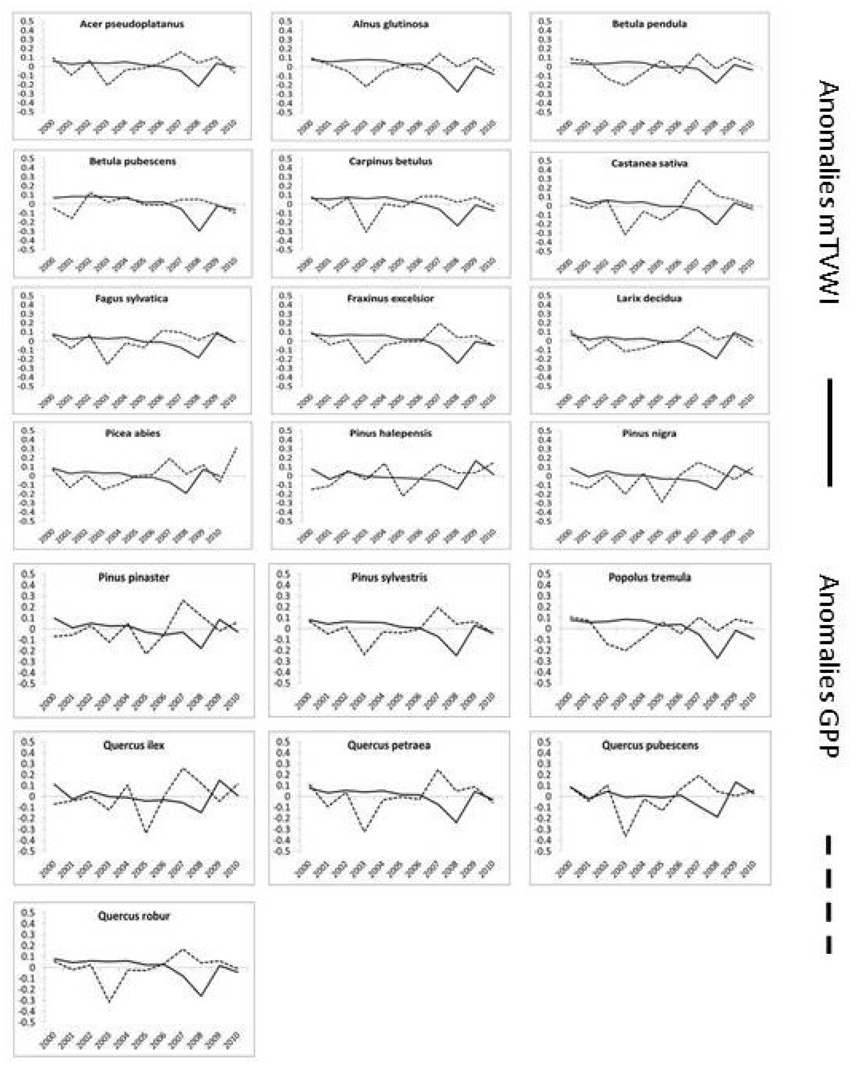
2.5. Anomalies Analysis
3. Results
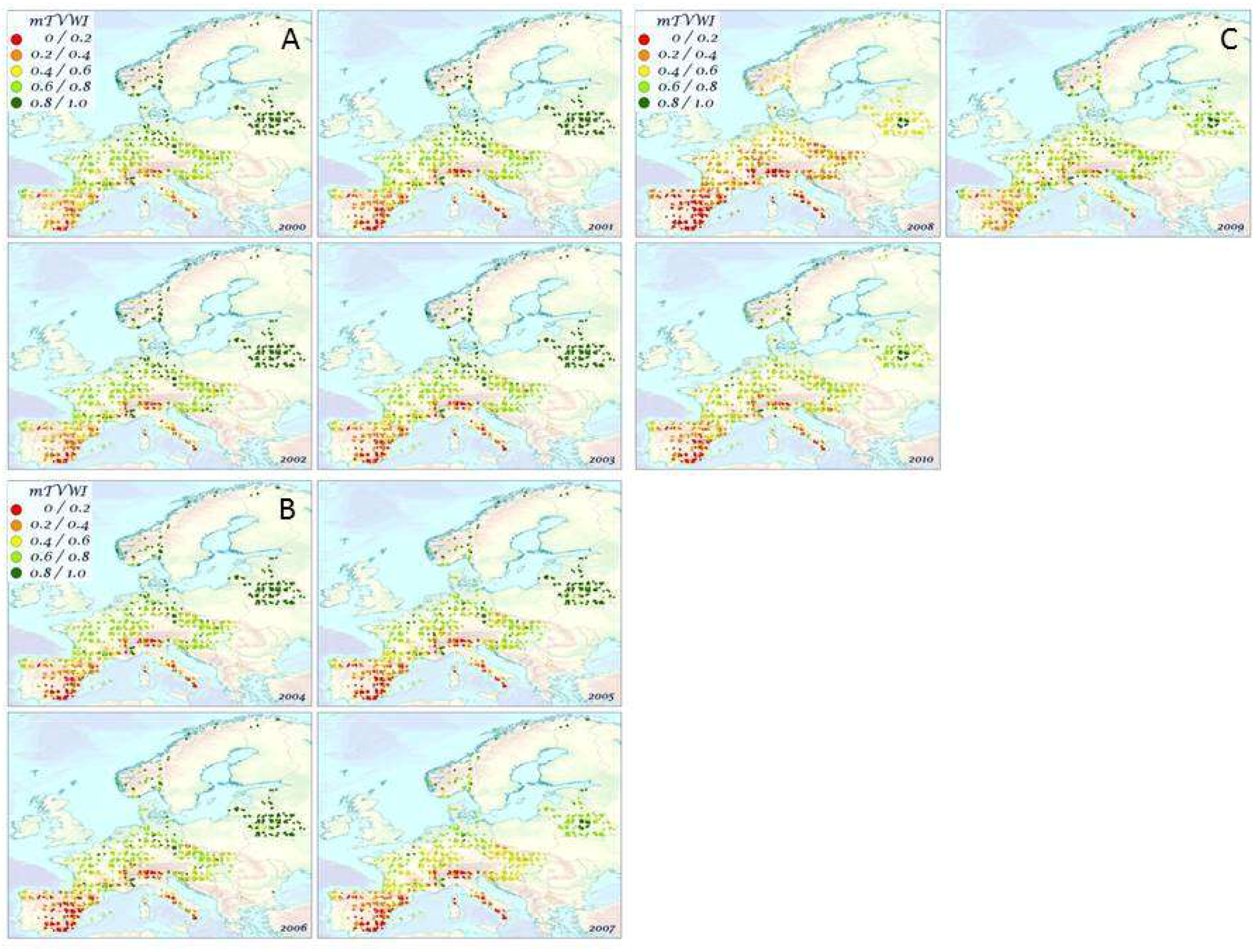
3.1. Space–Time Distribution Patterns of mTVWI in Europe
3.2. Correlation between GPP and mTVWI
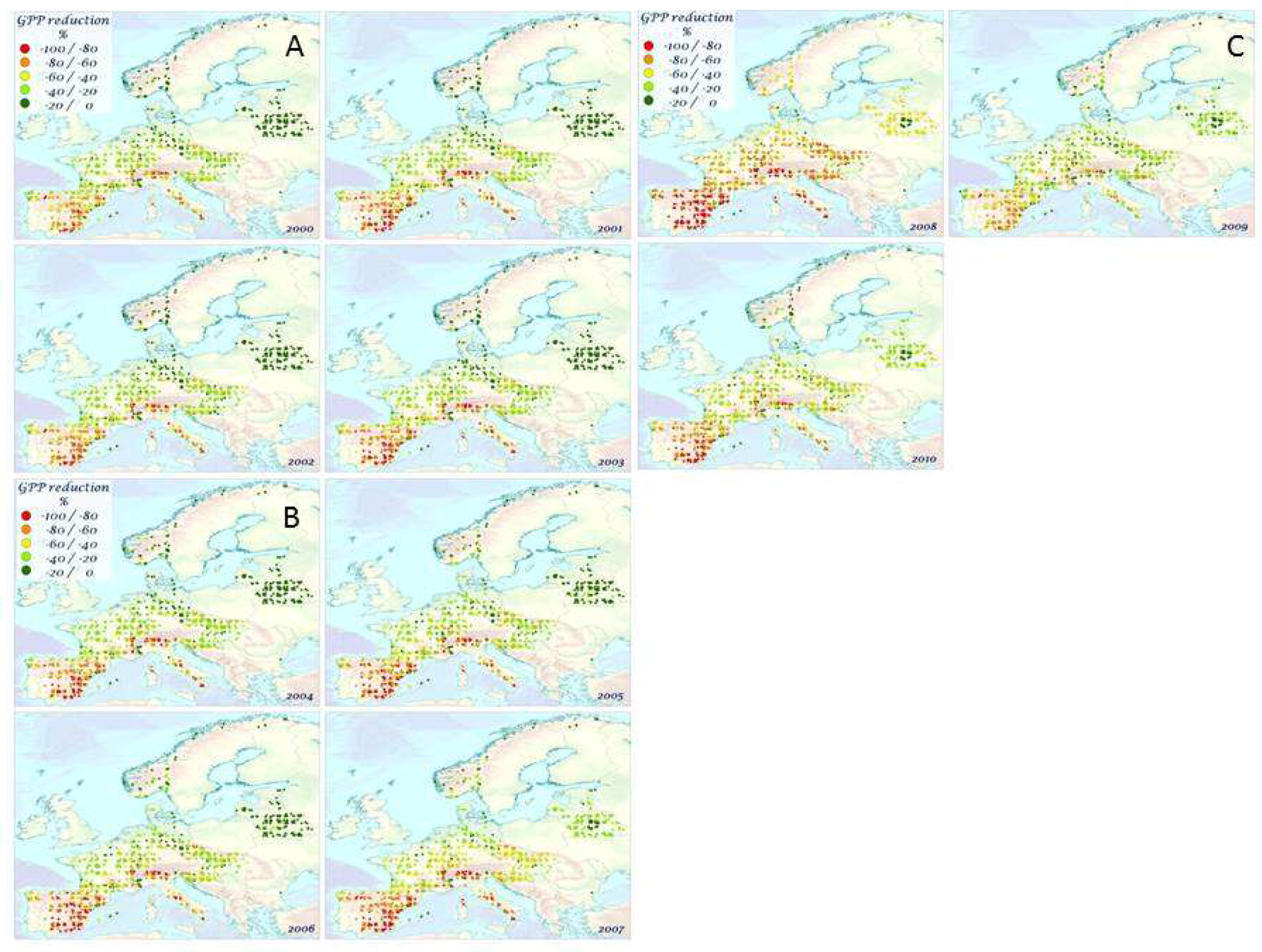
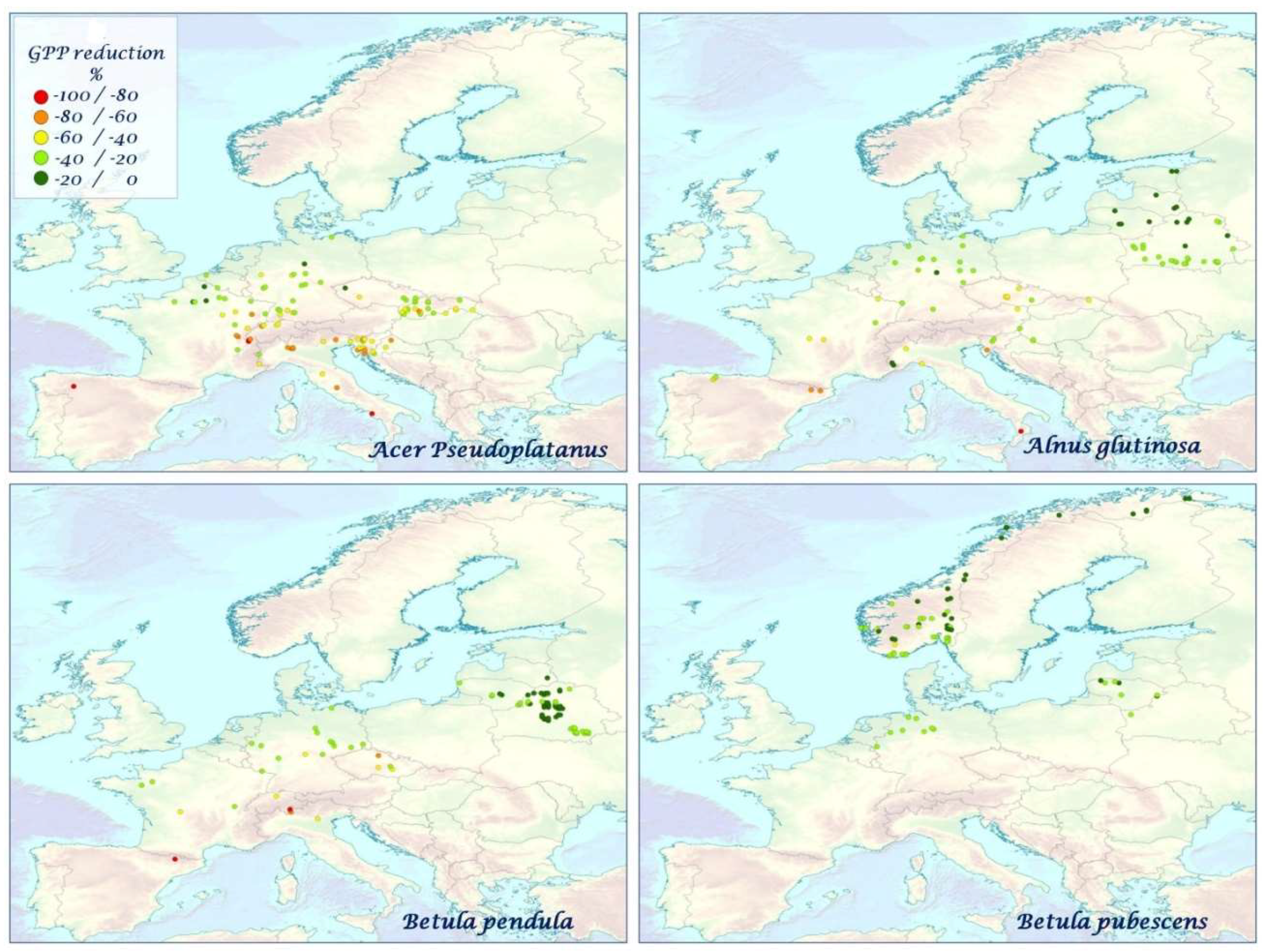
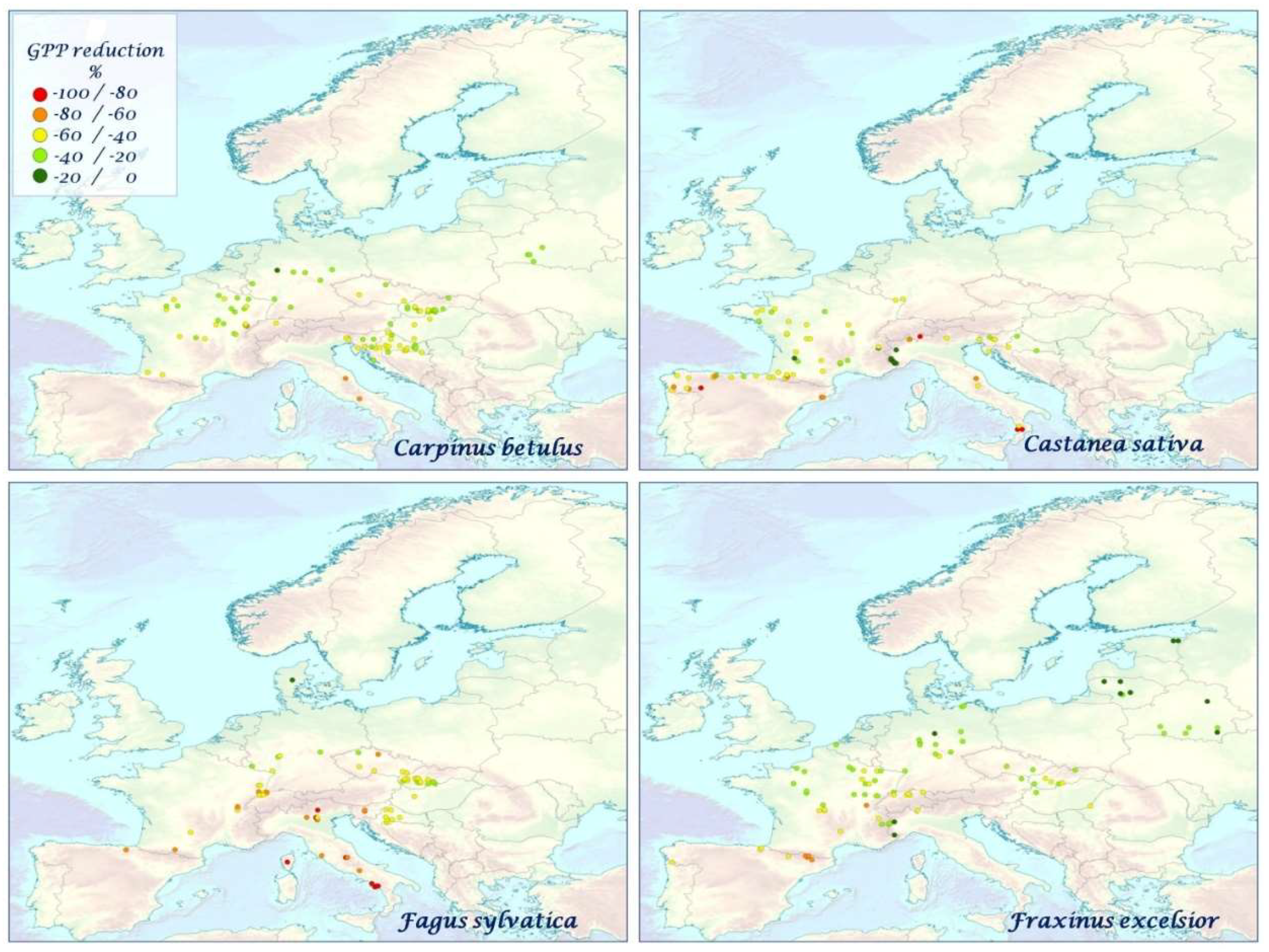
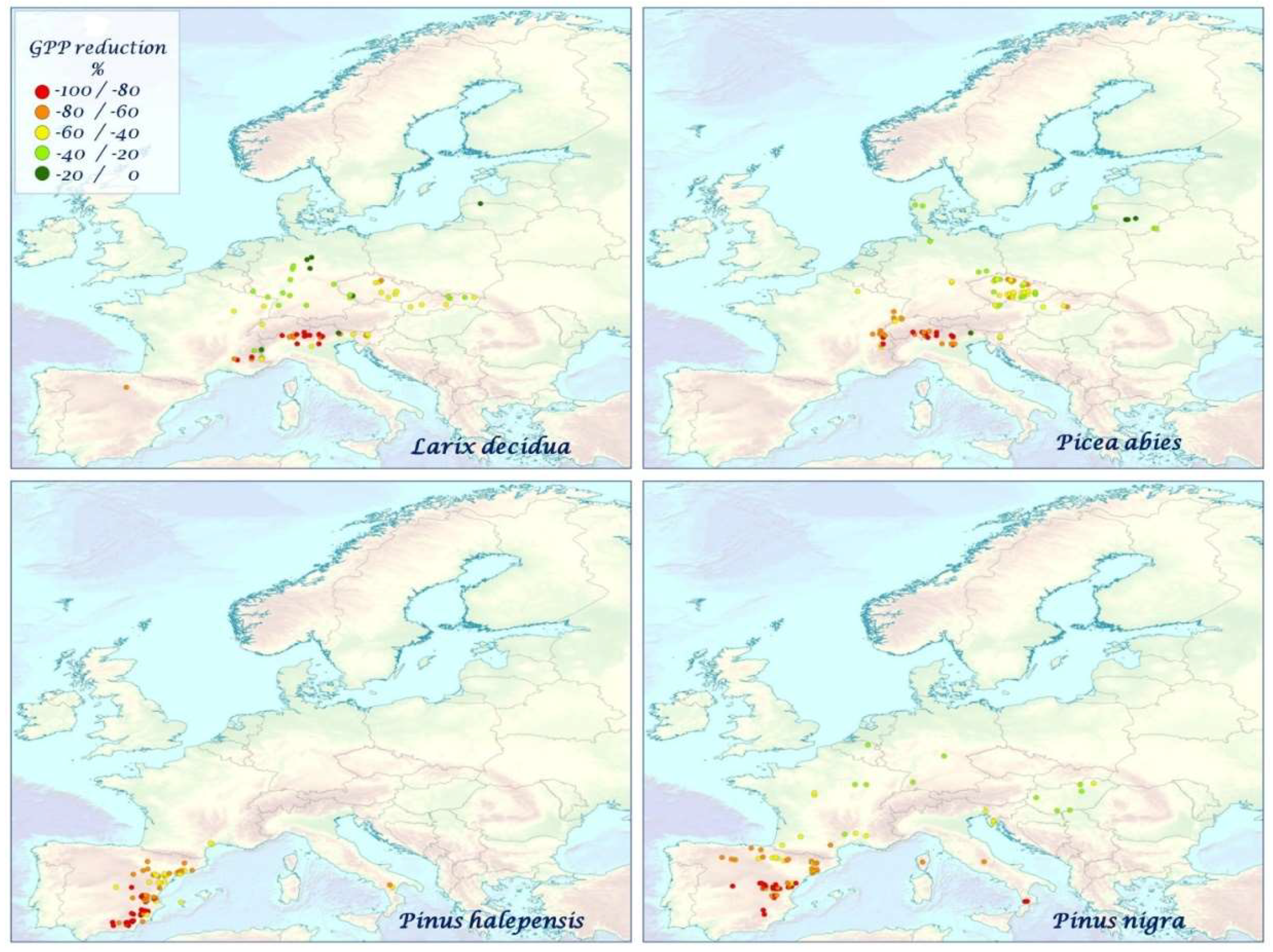
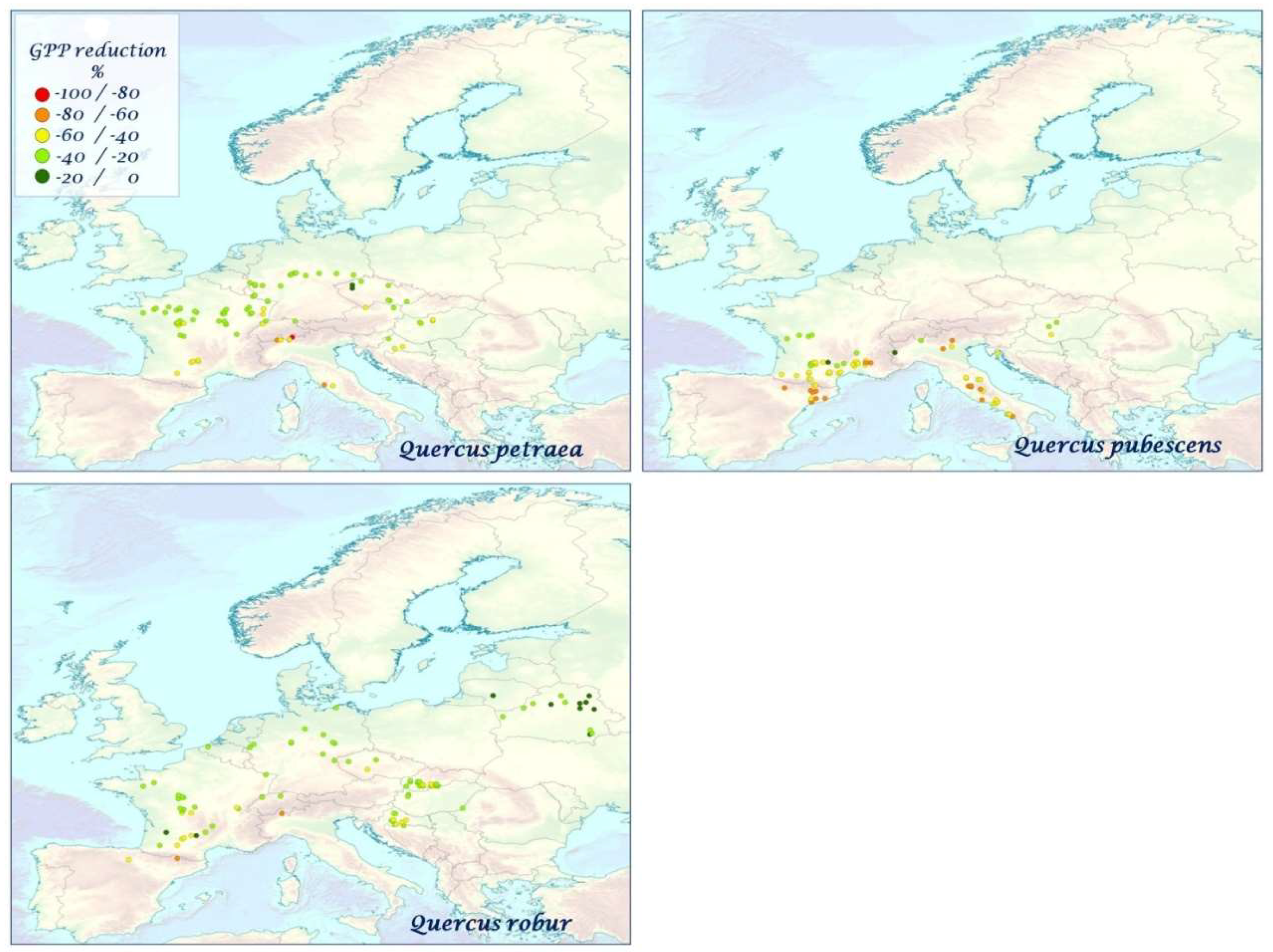
3.3. Impact of mTVWI on GPP
4. Discussion
4.1. Spatial and Temporal Distribution of mTVWI
4.2. Correlations, Impacts, and Anomalies of GPP and mTVWI
5. Conclusions
Supplementary Materials
Author Contributions
Funding
Acknowledgments
Conflicts of Interest
References
- Dai, A. Increasing drought under global warming in observations and models. Nat. Clim. Chang. 2013, 3, 52–58. [Google Scholar] [CrossRef]
- Huang, J.; Yu, H.; Guan, X.; Wang, G.; Guo, R. Accelerated dryland expansion under climate change. Nat. Clim. Chang. 2016, 6, 166–171. [Google Scholar] [CrossRef]
- Vicente-Serrano, S.M.; Camarero, J.J.; Azorın–Molina, C. Diverse responses of forest growth to drought timescales in the Northern Hemisphere. Glob. Ecol. Biogeogr. 2014, 23, 1019–1030. [Google Scholar] [CrossRef]
- Mavrakis, A.; Salvati, L. Analyzing the behavior of selected risk indexes during the 2007 Greek forest fires. Int. J. Environ. Res. 2015, 9, 831–840. [Google Scholar]
- Gao, X.; Giorgi, F. Increased aridity in the Mediterranean region under greenhouse gas forcing estimated from high resolution simulations with a regional climate model. Glob. Planet Chang. 2008, 62, 195–209. [Google Scholar] [CrossRef]
- Hertig, E.; Jacoboeit, J. Downscaling future climate change: Temperature scenarios for the Mediterranean area. Glob. Planet Chang. 2008, 63, 127–131. [Google Scholar] [CrossRef]
- Salvati, L.; Zitti, M.; Ceccarelli, T.; Perini, L. Building–up a synthetic index of land vulnerability to drought and desertification. Geogr. Res. 2009, 47, 280–291. [Google Scholar] [CrossRef]
- Salvati, L.; Perini, L.; Sabbi, A.; Bajocco, S. Climate aridity and land use changes: A regional-scale analysis. Geogr. Res. 2012, 50, 193–203. [Google Scholar] [CrossRef]
- Colantoni, A.; Ferrara, C.; Perini, L.; Salvati, L. Assessing Trends in Climate Aridity and Vulnerability to Soil Degradation in Italy. Ecol. Indic. 2015, 48, 599–604. [Google Scholar] [CrossRef]
- Michaletz, S.T.; Cheng, D.; Kerkhoff, A.J.; Enquist, B.J. Convergence of terrestrial plant production across global climate gradients. Nature 2014. [Google Scholar] [CrossRef]
- Cutini, A.; Manetti, M.C.; Mazza, G.; Moretti, V.; Salvati, L. Climate variability and growth rate of Pinus pinea L. in Castelporziano forest: An exploratory data analysis. Rend. Accad. Nazion. Lincei 2015, 26, 413–420. [Google Scholar] [CrossRef]
- Chu, C.; Bartlett, M.; Wang, Y.; He, F.; Weiner, J.; Chave, J.; Sack, L. Does climate directly influence NPP globally? Glob. Chang. Biol. 2016, 22, 12–24. [Google Scholar] [CrossRef]
- Salvati, R.; Salvati, L.; Ferrara, A.; Corona, P.; Barbati, A. Estimating the sensitivity to desertification of Italian forests. iForest 2014, 8, 287–294. [Google Scholar] [CrossRef]
- Zang, C.; Meier, C.H.; Dittmar, C.; Rothe, A.; Menzel, A. Patterns of drought tolerance in major European temperate forest trees: Climatic drivers and levels of variability. Glob. Chang. Biol. 2014, 20, 3767–3779. [Google Scholar] [CrossRef]
- Morales, P.; Hickler, T.; Rowell, D.P.; Smith, B.; Sykes, M.T. Changes in European ecosystem productivity and carbon balance driven by regional climate model output. Glob. Chang. Biol. 2007, 13, 108–122. [Google Scholar] [CrossRef]
- Anav, A.; Mariotti, A. Sensitivity of natural vegetation to climate change in the Euro-Mediterranean area. Clim. Res. 2011, 46, 277–292. [Google Scholar] [CrossRef]
- Barbeta, A.; Mejía-Chang, M.; Ogaya, R.; Voltas, J.; Dawson, T.E.; Penuelas, J. The combined effects of a long–term experimental drought and an extreme drought on the use of plant-water sources in a Mediterranean forest. Glob. Chang. Biol. 2014, 21, 1213–1225. [Google Scholar] [CrossRef]
- Sicard, P.; Dalstein-Richier, L. Health and vitality assessment of two common pine species in the context of climate change in southern Europe. Environ. Res. 2015, 137, 235–245. [Google Scholar] [CrossRef]
- Allen, C.D.; Macalady, A.K.; Chenchouni, H.; Bachelet, D.; McDowell, N.; Vennetier, M.; Kitzberger, T.; Rigling, A.; Breshears, D.D.; Hogg, E.H.; et al. A global overview of drought and heat-induced tree mortality reveals emerging climate change risks for forests. For. Ecol. Manag. 2010, 259, 660–684. [Google Scholar] [CrossRef]
- Mueller, R.C.; Scudder, C.M.; Porter, M.E.; Talbot, T.R.; Gehring, C.A.; Whitham, T.G. Differential tree mortality in response to severe drought: Evidence for long-term vegetation shifts. J. Ecol. 2005, 93, 1085–1093. [Google Scholar] [CrossRef]
- Breshears, D.D.; Cobb, N.S.; Rich, P.M.; Price, K.P.; Allen, C.D.; Balice, R.G.; Romme, W.H.; Kastens, J.H.; Floyd, M.L.; Belnap, J.; et al. Regional vegetation die–off in response to global-change-type drought. Proc. Natl. Acad. Sci. USA 2005, 102, 15144–15148. [Google Scholar] [CrossRef]
- Andreu, L.; Gutiérrez, E.; Macias, M.; Ribas, M.; Bosch, O.; Camarero, J.J. Climate increases regional tree-growth variability in Iberian pine forests. Glob. Chang. Biol. 2007, 13, 804–815. [Google Scholar] [CrossRef]
- Peng, C.; Ma, Z.; Lei, X.; Zhu, Q.; Chen, H.; Wang, W.; Liu, S.; Li, W.; Fang XZhou, X. A drought–induced pervasive increase in tree mortality across Canada’s boreal forests. Nat. Clim. Chang. 2011, 1, 467–471. [Google Scholar] [CrossRef]
- Granier, A.; Reichestein, M.; Brèda, N.; Janssens, I.A.; Falge, E.; Ciais, P.; Grünwald, T.; Aubinet, T.; Berbigier, P.; Bernhofer, C.; et al. Evidence for soil water control on carbon and water dynamics in European forests during the extremely dry year: 2003. Agric. For. Meteorol. 2007, 143, 123–145. [Google Scholar] [CrossRef]
- Friend, A.D.; Lucht, W.; Rademacher, T.T.; Keribin, R.; Betts, R.; Cadule, P.; Ciais, P.; Clark, D.B.; Dankers, R.; Falloon, P.D.; et al. Carbon residence time dominates uncertainty in terrestrial vegetation responses to future climate and atmospheric CO2. Proc. Natl. Acad. Sci. USA 2014, 111, 3280–3285. [Google Scholar] [CrossRef] [PubMed]
- Allen, C.D.; Breshears, D.D.; McDowell, N.G. On underestimation of global vulnerability to tree mortality and forest die–off from hotter drought in the Anthropocene. Ecosphere 2015, 6, 1–55. [Google Scholar] [CrossRef]
- McDowell, N.G.; Williams, A.P.; Xu, C.; Pockman, W.T.; Dickman, L.T.; Sevanto, S.; Pangle, R.; Limousin, J.; Plaut, J.; Mackay, D.S.; et al. Multi–scale predictions of massive conifer mortality due to chronic temperature rise. Nat. Clim. Chang. 2016, 6, 295–300. [Google Scholar] [CrossRef]
- Ayres, M.P.; Lombardero, M.J. Assessing the consequences of global change for forest disturbances for herbivores and pathogens. Sci. Total Environ. 2000, 262, 263–286. [Google Scholar] [CrossRef]
- Bachelet, D.; Neilson, R.P.; Hickler, T.; Drapek, R.J.; Lenihan, J.M.; Sykes, M.T.; Smith, B.; Sitch, S.; Thonicke, K. Simulating past and future dynamics of natural ecosystems in the United States. Glob. Biogeochem. Cycles 2003, 17, 1045. [Google Scholar] [CrossRef]
- Lucht, W.; Schaphoff, S.; Erbrecht, T.; Heyder, U.; Cramer, W. Terrestrial vegetation redistribution and carbon balance under climate change. Carbon Balance Manag. 2006, 1, 6. [Google Scholar] [CrossRef]
- Scholze, M.; Knorr, W.; Arnell, N.W.; Prentice, I. A climate–change risk analysis for world ecosystems. Proc. Natl. Acad. Sci. USA 2006, 103, 13116–13120. [Google Scholar] [CrossRef] [PubMed]
- Lloyd, A.H.; Bunn, A.G. Responses of the circumpolar boreal forest to 20th century climate variability. Environ. Res. Lett. 2007, 2, 045013. [Google Scholar] [CrossRef]
- Cleverly, J.; Eamus, D.; Restrepo Coupe, N.; Chen, C.; Maes, W.; Li, L.; Faux, R.; Santini, N.S.; Rumman, R.; Yu, Q.; et al. Soil moisture controls on phenology and productivity in a semi–arid critical zone. Sci. Total Environ. 2016, 568, 1227–1237. [Google Scholar] [CrossRef] [PubMed]
- Nemani, R.R.; Keeling, C.D.; Hashimoto, H.; Jolly, W.M.; Piper, S.C.; Tucker, C.J.; Myneni, R.B.; Running, S.W. Climate–Driven Increases in Global Terrestrial Net Primary Production from 1982 to 1999. Science 2003, 300, 1560–1563. [Google Scholar] [CrossRef] [PubMed]
- Murray-Tortarolo, G.; Friedlingstein, P.; Sitch, S.; Seneviratne, S.I.; Fletcher, I.; Mueller, B.; Greve, P.; Anav, A.; Liu, Y.; Ahlström, A.; et al. The dry season intensity as a key driver of NPP trends. Geophys. Res. Lett. 2016, 43, 2632–2639. [Google Scholar] [CrossRef]
- Salvati, L.; Petitta, M.; Ceccarelli, T.; Perini, L.; Di Battista, F.; Venezian Scarascia, M.E. Italy’s renewable water resources as estimated on the basis of the monthly water balance. Irr. Drain 2008, 57, 507–515. [Google Scholar] [CrossRef]
- Moretti, V.; Di Bartolomei, R.; Sorgi, T.; Aromolo, R.; Salvati, L. Soil water deficit and climate conditions during the dry season along the coastal–inland gradient in Castelporziano Forest, central Italy. Rend. Accad. Naz. Lincei 2015, 26, 283–288. [Google Scholar] [CrossRef]
- Wang, T.; Franz, T.E.; Yue, W.; Szilagyi, J.; Zlotnik, V.A.; You, J.; Chen, X.; Shulski, M.D.; Young, A. Feasibility analysis of using inverse modeling for estimating natural groundwaterrecharge from a large-scale soil moisture monitoring network. J. Hydrol. 2016, 533, 250–265. [Google Scholar] [CrossRef]
- Bittelli, M. Measuring soil water content: A review. HortTechnology 2011, 21, 293–300. [Google Scholar] [CrossRef]
- Zhang, D.; Tang, R.; Zhao, W.; Tang, B.; Wu, H.; Shao, K.; Li, Z.L. Surface Soil Water Content Estimation from Thermal Remote Sensing based on the Temporal Variation of Land Surface Temperature. Remote Sens. 2014, 6, 3170–3187. [Google Scholar] [CrossRef]
- Zhu, Y.; Wang, Y.; Shao, M.; Horton, R. Estimating soil water content from surface digital image gray level measurements under visible spectrum. Can. J. Soil Sci. 2011, 91, 69–76. [Google Scholar] [CrossRef]
- Kerr, Y.H.; Waldteufel, P.; Wigneron, J.P.; Delwart, S.; Cabot, F.; Boutin, J.; Escorihuela, M.J.; Font, J.; Reul, N.; Gruhier, C.; et al. The SMOS mission: New tool for monitoring key elements of the global water cycle. Proc. IEEE Inst. Electr. Electron. Eng. 2010, 98, 666–687. [Google Scholar] [CrossRef]
- Qiu, B.; Xue, Y.; Fisher, J.B.; Guo, W.; Berry, J.A.; Zhang, Y. Satellite chlorophyll fluorescence and soil moisture observations lead to advances in the predictive understanding of global terrestrial coupled carbon-water cycles. Glob. Biogeochem. Cycles 2018, 32, 360–375. [Google Scholar] [CrossRef]
- Moran, M.S.; Peters–Lidard, C.D.; Watts, J.M.; McElroy, J. Estimating soil moisture at the watershed scale with satellite–based radar and land surface models. Can. J. Remote Sens. 2004, 30, 805–826. [Google Scholar] [CrossRef]
- Hassan, Q.K.; Bourque, C.P.; Meng, F.R.; Cox, R.M. A wetness index using terrain–corrected surface temperature and normalized difference vegetation index derived from standard MODIS products: An evaluation of its use in a humid forest–dominated region of eastern Canada. Sensors 2007, 7, 2028–2048. [Google Scholar] [CrossRef]
- Vitale, M.; Proietti, C.; Cionni, I.; Fischer, R.; De Marco, A. Random forests analysis: A useful tool for defining the relative importance of environmental conditions on crown defoliation. Water Air Soil Pollut. 2014, 225, 1–17. [Google Scholar] [CrossRef]
- Michel, A.; Seidling, W. (Eds.) Forest Condition in Europe: 2017 Technical Report of ICP Forests. Report under the UNECE Convention on Long-Range Transboundary Air Pollution (CLRTAP); BFW Dokumentation 24/2017; BFW Austrian Research Centre for Forests: Vienna, Austria, 2017; 128p. [Google Scholar]
- Rossini, M.; Panigada, C.; Meroni, M.; Colombo, R. Assessment of oak forest condition based on leaf biochemical variables and chlorophyll fluorescence. Tree Physiol. 2006, 26, 1487–1496. [Google Scholar] [CrossRef] [PubMed]
- Fischer, R.; Lorenz, M. Forest Condition in Europe, 2011 Technical Report of ICP Forests and FutMon. Work Report of the Institute for World Forestry 2011/1; ICP Forests: Hamburg, Germany, 2011; p. 212. [Google Scholar]
- De Marco, A.; Proietti, C.; Cionni, I.; Fischer, R.; Screpanti, A.; Vitale, M. Future impacts of nitrogen deposition and climate change scenarios on forest crown defoliation. Environ. Pollut. 2014, 194, 171–180. [Google Scholar] [CrossRef]
- Ferretti, M.; Marchetto, A.; Arisci, S.; Bussotti, F.; Calderisi, M.; Carnicelli, S.; Cecchini, G.; Fabbio, G.; Bertini, G.; Matteucci, G.; et al. On the tracks of Nitrogen deposition effects on temperate forests at their southern European range—An observational study from Italy. Glob. Chang. Biol. 2014, 20, 3423–3438. [Google Scholar] [CrossRef]
- Badea, O. Manual on Methodology for Long-Term Monitoring of Forest Ecosystems Status under Air Pollution and Climate Change Influence ed; Editura Silvică: Bucharest, Romania, 2008. [Google Scholar]
- ICP Forests. International Cooperative Programme on Assessment and Monitoring of Air Pollution Effects on Forests. Manual on Methods and Criteria for Harmonized Sampling, Assessment, Monitoring and Analysis of the Effects of Air Pollution on Forests, Part I (Federal Research Center for Forestry and Forest Products; ICP Forests: Hamburg, Germany, 2010. [Google Scholar]
- Zhao, M.; Heinsch, F.A.; Nemani, R.R.; Running, S.W. Improvements of the MODIS terrestrial gross and net primary production global data set. Remote Sens. Environ. 2005, 95, 164–176. [Google Scholar] [CrossRef]
- Turner, D.P.; Ritts, W.D.; Cohen, W.B.; Gower, S.T.; Running, S.W.; Zhao, M.; Costa, M.H.; Kirschbaum, A.A.; Ham, J.M.; Saleska, S.R.; et al. Evaluation of MODIS NPP and GPP products across multiple biomes. Remote Sens Environ. 2006, 102, 282–292. [Google Scholar] [CrossRef]
- Running, S.W.; Nemani, R.R.; Heinsch, F.A.; Zhao, M.; Reeves, M.; Hashimoto, H. A continuous satellite–derived measure of global terrestrial primary production. Bioscience 2004, 54, 547–560. [Google Scholar] [CrossRef]
- Heinsch, F.A.; Reeves, M.; Votava, P.; Kang, S.; Milesi, C.; Zhao, M.; Glassy, J.; Jolly, W.M.; Loehman, R.; Bowker, C.F.; et al. GPP and NPP (MOD17A2/A3) Products NASA MODIS Land Algorithm. In MOD17 User’s Guide; MODIS Land Team: Washington, DC, USA, 2003; pp. 1–57. [Google Scholar]
- Reed, B.C.; Brown, J.F.; VanderZee, D.; Loveland, T.R.; Merchant, J.W.; Ohlen, D.O. Measuring phenological variability from satellite imagery. J. Veg. Sci. 1994, 5, 703–714. [Google Scholar] [CrossRef]
- Stevens, J. Partial and Semipartial Correlations. 2003. Available online: www.uoregon.edu/~stevensj/MRA/partial.pdf (accessed on 2010 February 10).
- Vargas, R.; Baldocchi, D.D.; Bahn, M.; Hanson, P.J.; Hosman, K.P.; Kulmala, L.; Pumpanen, J.; Yang, B. On the multi–temporal correlation between photosynthesis and soil CO2 efflux: Reconciling lags and observations. New Phytol. 2011, 191, 1006–1017. [Google Scholar] [CrossRef]
- Heinemeyer, A.; Wilkinson, M.; Vargas, R.; Subke, J.A.; Casella, E.; Morison, J.I.L.; Ineson, P. Exploring the “overflow tap” theory: Linking forest soil CO2 fluxes and individual mycorrhizosphere components to photosynthesis. Biogeosciences 2012, 9, 79–95. [Google Scholar] [CrossRef]
- Proietti, C.; Anav, A.; De Marco, A.; Sicard, P.; Vitale, M. A multi–sites analysis on the ozone effects on Gross Primary Production of European forests. Sci. Total Environ. 2016, 556, 1–11. [Google Scholar] [CrossRef]
- Fares, S.; Vargas, R.; Detto, M.; Goldstein, A.H.; Karlik, J.; Paoletti, E.; Vitale, M. Tropospheric ozone reduces carbon assimilation in trees: Estimates from analysis of continuous flux measurements. Glob. Chang. Biol. 2013, 19, 2427–2443. [Google Scholar] [CrossRef] [PubMed]
- Ceccarelli, T.; Bajocco, S.; Perini, L.; Salvati, L. Urbanisation and Land Take of High Quality Agricultural Soils—Exploring Long–term Land Use Changes and Land Capability in Northern Italy. Int. J. Environ. Res. 2014, 8, 181–192. [Google Scholar]
- Pili, S.; Grigoriadis, E.; Carlucci, M.; Clemente, M.; Salvati, L. Towards Sustainable Growth? A Multi–criteria Assessment of (Changing) Urban Forms. Ecol. Indic. 2017, 76, 71–80. [Google Scholar] [CrossRef]
- Chen, P.Y.; Popovich, P.M. Correlation: Parametric and Nonparametric Measures; Sage Publications: Thousand Oaks, CA, USA, 2002. [Google Scholar]
- Duvernoy, I.; Zambon, I.; Sateriano, A.; Salvati, L. Pictures from the Other Side of the Fringe: Urban Growth and Peri–urban Agriculture in a Post–industrial City (Toulouse, France). J. Rural Stud. 2018, 57, 25–35. [Google Scholar] [CrossRef]
- Anav, A.; Menut, L.; Khvorostyanov, D.; Viovy, N. Impact of tropospheric ozone on the Euro-Mediterranean vegetation. Glob. Chang. Biol. 2011, 17, 2342–2359. [Google Scholar] [CrossRef]
- Beniston, M. The 2003 heat wave in Europe: A shape of things to come? An analysis based on Swiss climatological data and model simulations. Geophys. Res. Lett. 2004, 31. [Google Scholar] [CrossRef]
- Maracchi, G.; Sirotenko OBindi, M. Impacts of Present and Future Climate Variability on Agriculture and Forestry in the Temperate Regions: Europe. Clim. Chang. 2005, 70, 117. [Google Scholar] [CrossRef]
- Vicente-Serrano, S.M.; Cuadrat-Prats, J.M.; Romo, A. Aridity influence on vegetation patterns in the middle Ebro Valley (Spain): Evaluation by means of AVHRR images and climate interpolation techniques. J. Arid Environ. 2006, 66, 353–375. [Google Scholar] [CrossRef]
- Jump, A.S.; Hunt, J.M.; Peñuelas, J. Rapid climate change–related growth decline at the southern range edge of Fagus sylvatica. Glob. Chang. Biol. 2006, 12, 2163–2174. [Google Scholar] [CrossRef]
- Sarris, D.; Christodoulakis, D.; Körner, C. Recent decline in precipitation and tree growth in the eastern Mediterranean. Glob. Chang. Biol. 2007, 13, 1187–1200. [Google Scholar] [CrossRef]
- Martínez-Vilalta, J.; Lopez, B.C.; Adell, N.; Badiella, L.; Ninyerola, M. Twentieth century increase of Scots pine radial growth in NE Spain shows strong climate interactions. Glob. Chang. Biol. 2008, 14, 2868–2881. [Google Scholar] [CrossRef]
- ICP Forests. International Cooperative Programme on Assessment and Monitoring of Air Pollution Effects on Forests Executive Report; ICP Forests: Hamburg, Germany, 2008; printed in Germany. [Google Scholar]
- De Marco, A.; Sicard, P.; Fares, S.; Tuovinen, J.P.; Anav, A.; Paoletti, E. Assessing the role of soil water limitation in determining the Phytotoxic Ozone Dose (PODY) thresholds. Atmos. Environ. 2016, 147, 88–97. [Google Scholar] [CrossRef]
- Pasho, E.; Camarero, J.J.; de Luis, M.; Vicente-Serrano, S.M. Impacts of drought at different time scales on forest growth across a wide climatic gradient in northeastern Spain. Agric. For. Meteorol. 2011, 151, 1800–1811. [Google Scholar] [CrossRef]
- Araminiene, W.; Sicard, P.; Anav, A.; Agathokleous, E.; Stakėnas, V.; De Marco, A.; Varnagirytė-Kabašinskienė, I.; Paoletti, E.; Girgždienė, R. Trends and inter-relationships of ground-level ozone metrics and forest health in Lithuania. Sci. Total Environ. 2019, 658, 1265–1277. [Google Scholar] [CrossRef]
- Carnicer, J.; Coll, M.; Ninyerola, M.; Pons, X.; Sanchez, G.; Penuelas, J. Widespread crown condition decline, food web disruption, and amplified tree mortality with increased climate change-type drought. Proc. Natl. Acad. Sci. USA 2011, 108, 1474–1478. [Google Scholar] [CrossRef] [PubMed]
- Corcuera, L.; Camarero, J.J.; Gil-Pelegrín, E. Effects of a severe drought on Quercus ilex radial growth and xylem anatomy. Trees-Struct. Funct. 2004, 18, 83–92. [Google Scholar]
- Montserrat–Martí, G.; Camarero, J.J.; Palacio, S.; Pérez–Rontomé, C.; Milla, R.; Albuixech, J.; Maestro, M. Summer–drought constrains the phenology and growth of two coexisting Mediterranean oaks with contrasting leaf habit: Implications for their persistence and reproduction. Trees 2009, 23, 787–799. [Google Scholar] [CrossRef]
- Gutiérrez, E.; Campelo, F.; Camarero, J.J.; Ribas, M.; Muntán, E.; Nabais, C.; Freitas, H. Climate controls act at different scales on the seasonal pattern of Quercus ilex L. stem radial increments in NE Spain. Trees Struct. Funct. 2011. [Google Scholar] [CrossRef]
- Ciais, P.; Reichstein, M.; Viovy, N.; Granier, A.; Ogée, J.; Allard, V.; Aubinet, M.; Buchmann, N.; Bernhofer, C.; Carrara, A.; et al. Europe–wide reduction in primary productivity caused by the heat and drought in 2003. Nature 2005, 437, 529–533. [Google Scholar] [CrossRef] [PubMed]
- Canadell, J.G.; Le Quéré, C.; Raupach, M.R.; Field, C.B.; Buitenhuis, E.T.; Ciais, P.; Conway, T.J.; Gillett, N.P.; Houghton, R.A.; Marland, G. Contributions to accelerating atmospheric CO2 growth from economic activity, carbon intensity, and efficiency of natural sinks. Proc. Natl. Acad. Sci. USA 2007, 104, 18866–18870. [Google Scholar] [CrossRef] [PubMed]
- Atkinson, M.D. Betula pendula Roth (B. verrucosa Ehrh.) and B. pubescens Ehrh. J. Ecol. 1992, 80, 837–870. [Google Scholar] [CrossRef]
- Bernetti, G. Selvicoltura Speciale; Unione Tipografico-Editrice Torinese: Torino, Italy, 1995; ISBN 8802048673. [Google Scholar]
- Lebourgeois, F.; Breda, N.; Ulrich, E.; Granier, A. Climate-tree-growth relationships of European beech (Fagus sylvatica L.) in the French Permanent Plot Network (RENECOFOR). Trees 2005, 19, 385–401. [Google Scholar] [CrossRef]
- Zhao, M.; Running, S.W. Drought–induced reduction in global terrestrial net primary production from 2000 through 2009. Science 2010, 329, 940–943. [Google Scholar] [CrossRef]
- Churkina, G.; Running, S.W. Contrasting climatic controls on the estimated productivity of global terrestrial biomes. Ecosystems 1998, 1, 206–215. [Google Scholar] [CrossRef]
- Linares, J.C.; Delgado–Huertas, A.; Carreira, J.A. Climatic trends and different drought adaptive capacity and vulnerability in a mixed Abies pinsapo–Pinus halepensis forest. Clim. Chang. 2010, 105, 67–90. [Google Scholar] [CrossRef]
- Gruber, A.; Strobl, S.; Veit, B.; Oberhuber, W. Impact of drought on the temporal dynamics of wood formation in Pinus sylvestris. Tree Physiol. 2010, 30, 490–501. [Google Scholar] [CrossRef] [PubMed]
- Koepke, D.F.; Kolb, T.E.; Adams, H.D. Variation in woody plant mortality and dieback from severe drought among soils, plant groups, and species within a northern Arizona ecotone. Glob. Chang. Ecol. 2010, 163, 1079–1090. [Google Scholar] [CrossRef] [PubMed]
- Boisvenue, C.; Running, S.W. Impacts of climate change on natural forest productivity—Evidence since the middle of the 20th century. Glob. Chang. Biol. 2006, 12, 862–882. [Google Scholar] [CrossRef]
- Bonan, G.B. Forests and Climate Change: Forcings, Feedbacks, and the Climate Benefits of Forests. Science 2008, 320, 1444–1449. [Google Scholar] [CrossRef]
- Sperry, J.S.; Hacke, U.G.; Oren, R.; Comstock, J.P. Water deficits and hydraulic limits to leaf water supply. Plant Cell Environ. 2002, 25, 251–263. [Google Scholar] [CrossRef] [PubMed]


| SPECIES | r (GPP, mTVWI) | ||||||||||
|---|---|---|---|---|---|---|---|---|---|---|---|
| 2000 | 2001 | 2002 | 2003 | 2004 | 2005 | 2006 | 2007 | 2008 | 2009 | 2010 | |
| Conifers | 0.15 | 0.15 | 0.13 | 0.09 | 0.15 | 0.13 | 0.08 | 0.12 | 0.12 | 0.10 | 0.10 |
| Larix decidua (N = 72) | 0.27 | 0.34 | 0.35 | 0.19 | 0.40 | 0.38 | 0.40 | 0.38 | 0.33 | 0.39 | 0.35 |
| Picea abies (N = 97) | −0.03 | 0.03 | −0.04 | −0.20 | 0.04 | −0.10 | −0.09 | −0.02 | −0.01 | 0.001 | −0.11 |
| Pinus halepensis (N = 82) | 0.11 | 0.09 | 0.11 | 0.08 | 0.07 | 0.07 | 0.09 | −0.02 | 0.05 | 0.11 | 0.12 |
| Pinus nigra (N = 89) | 0.26 | 0.25 | 0.23 | 0.17 | 0.18 | 0.26 | 0.15 | 0.16 | 0.17 | 0.21 | 0.15 |
| Pinus pinaster (N = 87) | 0.46 | 0.47 | 0.46 | 0.43 | 0.45 | 0.50 | 0.44 | 0.46 | 0.48 | 0.38 | 0.36 |
| Pinus sylvestris (N = 77) | −0.39 | −0.40 | −0.38 | −0.38 | −0.36 | −0.32 | −0.39 | −0.39 | −0.34 | −0.32 | −0.29 |
| Broad-leaf deciduous | −0.20 | −0.20 | −0.27 | −0.25 | −0.22 | −0.21 | −0.25 | −0.22 | −0.18 | −0.10 | −0.15 |
| Acer pseudoplatanus (N = 100) | −0.30 | −0.36 | −0.33 | −0.37 | −0.28 | −0.27 | −0.36 | −0.32 | −0.31 | −0.25 | −0.25 |
| Alnus glutinosa (N = 78) | −0.44 | −0.44 | −0.46 | −0.43 | −0.43 | −0.34 | −0.34 | −0.43 | −0.09 | −0.09 | −0.18 |
| Betula pendula (N = 97) | 0.45 | 0.56 | 0.46 | 0.46 | 0.61 | 0.42 | 0.24 | 0.22 | 0.09 | 0.12 | −0.05 |
| Betula pubescens(N = 71) | 0.03 | 0.07 | 0.02 | −0.004 | −0.10 | −0.21 | −0.19 | −0.01 | −0.16 | −0.003 | −0.13 |
| Carpinus betulus (N = 92) | −0.25 | −0.36 | −0.30 | −0.41 | −0.34 | −0.32 | −0.26 | −0.29 | −0.09 | 0.13 | −0.15 |
| Castanea sativa (N = 73) | 0.01 | −0.11 | −0.04 | −0.09 | −0.08 | −0.05 | −0.07 | −0.03 | 0.06 | 0.16 | 0.02 |
| Fagus sylvatica (N = 82) | −0.14 | −0.10 | −0.12 | −0.21 | 0.03 | −0.01 | −0.04 | −0.15 | −0.02 | 0.03 | 0.05 |
| Fraxinus excelsior (N = 88) | −0.27 | −0.30 | −0.35 | −0.28 | −0.30 | −0.28 | −0.30 | −0.34 | −0.29 | −0.24 | −0.30 |
| Populus tremula (N = 94) | −0.55 | −0.54 | −0.56 | −0.42 | −0.53 | −0.48 | −0.38 | −0.69 | −0.51 | −0.25 | −0.16 |
| Quercus petraea (N = 85) | 0.03 | −0.04 | −0.08 | −0.13 | −0.06 | −0.10 | −0.16 | −0.06 | −0.12 | −0.03 | −0.05 |
| Quercus pubescens (N = 75) | −0.19 | −0.29 | −0.32 | −0.36 | −0.29 | −0.18 | −0.12 | −0.20 | −0.18 | −0.03 | −0.11 |
| Quercus robur (N = 94) | −0.27 | −0.34 | −0.33 | −0.35 | −0.34 | −0.29 | −0.35 | −0.32 | −0.20 | −0.09 | −0.23 |
| Broad-leaf evergreen | 0.19 | 0.27 | 0.24 | 0.25 | 0.28 | 0.27 | 0.33 | 0.26 | 0.28 | 0.20 | 0.19 |
| Quercus ilex (N = 90) | 0.19 | 0.27 | 0.24 | 0.25 | 0.28 | 0.27 | 0.33 | 0.26 | 0.28 | 0.20 | 0.19 |
| SPECIES | rs (GPP, mTVWI) | ||||||||||
|---|---|---|---|---|---|---|---|---|---|---|---|
| 2000 | 2001 | 2002 | 2003 | 2004 | 2005 | 2006 | 2007 | 2008 | 2009 | 2010 | |
| Conifers | 0.26 | 0.28 | 0.23 | 0.16 | 0.24 | 0.29 | 0.21 | 0.26 | 0.23 | 0.22 | 0.16 |
| Larix decidua (N = 72) | 0.12 | 0.17 | 0.16 | −0.05 | 0.26 | 0.24 | 0.22 | 0.20 | 0.13 | 0.23 | 0.16 |
| Picea abies (N = 97) | −0.19 | −0.13 | −0.17 | −0.34 | −0.06 | −0.15 | −0.16 | −0.08 | −0.08 | −0.04 | −0.22 |
| Pinus halepensis (N = 82) | 0.19 | 0.22 | 0.18 | 0.20 | 0.19 | 0.14 | 0.17 | 0.05 | 0.12 | 0.19 | 0.16 |
| Pinus nigra (N = 89) | 0.25 | 0.22 | 0.20 | 0.13 | 0.15 | 0.34 | 0.23 | 0.18 | 0.27 | 0.31 | 0.21 |
| Pinus pinaster (N = 87) | 0.47 | 0.45 | 0.45 | 0.46 | 0.47 | 0.47 | 0.48 | 0.46 | 0.51 | 0.40 | 0.42 |
| Pinus sylvestris (N = 77) | −0.34 | −0.38 | −0.40 | −0.40 | −0.37 | −0.36 | −0.49 | −0.28 | −0.41 | −0.48 | −0.43 |
| Broad-leaf deciduous | −0.58 | −0.61 | −0.66 | −0.63 | −0.65 | −0.57 | −0.63 | −0.59 | −0.53 | −0.43 | −0.44 |
| Acer pseudoplatanus (N = 100) | −0.43 | −0.54 | −0.49 | −0.52 | −0.39 | −0.44 | −0.47 | −0.38 | −0.44 | −0.39 | −0.35 |
| Alnus glutinosa (N = 78) | −0.60 | −0.48 | −0.67 | −0.54 | −0.63 | −0.52 | −0.59 | −0.61 | −0.40 | −0.22 | −0.21 |
| Betula pendula (N = 97) | −0.39 | −0.27 | −0.54 | −0.42 | −0.45 | −0.42 | −0.48 | −0.35 | −0.26 | −0.26 | −0.08 |
| Betula pubescens(N = 71) | −0.56 | −0.55 | −0.50 | −0.50 | −0.52 | −0.48 | −0.53 | −0.60 | −0.60 | −0.44 | −0.36 |
| Carpinus betulus (N = 92) | −0.35 | −0.49 | −0.48 | −0.40 | −0.43 | −0.26 | −0.39 | −0.30 | −0.13 | 0.05 | −0.20 |
| Castanea sativa (N = 73) | −0.15 | −0.32 | −0.28 | −0.29 | −0.34 | −0.20 | −0.20 | −0.19 | −0.15 | 0.04 | −0.22 |
| Fagus sylvatica (N = 82) | −0.56 | −0.59 | −0.59 | −0.73 | −0.49 | −0.47 | −0.42 | −0.56 | −0.50 | −0.30 | −0.42 |
| Fraxinus excelsior (N = 88) | −0.49 | −0.52 | −0.56 | −0.53 | −0.59 | −0.47 | −0.52 | −0.55 | −0.48 | −0.46 | −0.44 |
| Populus tremula (N = 94) | −0.45 | −0.34 | −0.44 | −0.29 | −0.32 | −0.43 | −0.45 | −0.31 | −0.19 | −0.18 | −0.11 |
| Quercus petraea (N = 85) | 0.01 | −0.22 | −0.19 | −0.21 | −0.24 | −0.19 | −0.26 | −0.09 | −0.17 | −0.08 | −0.07 |
| Quercus pubescens (N = 75) | −0.25 | −0.31 | −0.37 | −0.43 | −0.39 | −0.25 | −0.20 | −0.20 | −0.18 | −0.07 | −0.09 |
| Quercus robur(N = 94) | −0.35 | −0.51 | −0.54 | −0.53 | −0.57 | −0.47 | −0.57 | −0.38 | −0.44 | −0.33 | −0.35 |
| Broad-leaf evergreen | 0.23 | 0.22 | 0.24 | 0.25 | 0.22 | 0.21 | 0.24 | 0.21 | 0.20 | 0.09 | 0.13 |
| Quercus ilex (N = 90) | 0.23 | 0.22 | 0.24 | 0.25 | 0.22 | 0.21 | 0.24 | 0.21 | 0.20 | 0.09 | 0.13 |
| SPECIES | GPP Reduction (%) | ||||||||||
|---|---|---|---|---|---|---|---|---|---|---|---|
| 2000 | 2001 | 2002 | 2003 | 2004 | 2005 | 2006 | 2007 | 2008 | 2009 | 2010 | |
| Conifers | −49.3 ± 21.88 | −56.9 ± 25.21 | −52.70 ± 23.57 | −55.53 ± 24.95 | −55.61 ± 25.27 | −59.55 ± 25.31 | −60.16 ± 26.51 | −63.76 ± 20.52 | −75.96 ± 15.19 | −48.34 ± 19.79 | −58.28 ± 20.57 |
| Larix decidua (N = 72) | −47.03 ± 26.80 | −52.55 ± 30.60 | −49.39 ± 29.58 | −52.17 ± 30.87 | −51.48 ± 30.86 | −54.92 ± 30.29 | −53.94 ± 29.90 | −61.32 ± 25.85 | −73.36 ± 18.01 | −44.48 ± 22.74 | −54.16 ± 22.50 |
| Picea abies (N = 97) | −46.81 ± 21.14 | −53.01 ± 23.95 | −50.89 ± 22.88 | −52.73 ± 24.68 | −52.40 ± 24.11 | −57.16 ± 24.67 | −57.40 ± 26.80 | −62.71 ± 19.87 | −74.80 ± 15.04 | −48.39 ± 23.29 | −55.68 ± 20.79 |
| Pinus halepensis (N = 82) | −60.97 ± 13.87 | −72.27 ± 15.21 | −64.11 ± 15.04 | −69.11 ± 13.14 | −70.40 ± 14.33 | −71.42 ± 15.97 | −72.19 ± 17.94 | −74.34 ± 11.54 | −83.21 ± 9.55 | −51.95 ± 13.39 | −67.27 ± 16.19 |
| Pinus nigra (N = 89) | −57.18 ± 19.34 | −66.86 ± 21.72 | −60.91 ± 20.76 | −65.13 ± 21.87 | −65.46 ± 22.80 | −69.38 ± 23.43 | −69.50 ± 25.00 | −71.85 ± 18.04 | −80.98 ± 14.90 | −54.54 ± 19.29 | −64.51 ± 20.11 |
| Pinus pinaster (N = 87) | −49.86 ± 21.08 | −58.87 ± 22.29 | −54.76 ± 21.36 | −57.23 ± 21.51 | −56.95 ± 22.31 | −62.92 ± 22.41 | −65.48 ± 23.40 | −62.71 ± 18.68 | −77.25 ± 13.88 | −51.19 ± 17.28 | −62.38 ± 18.85 |
| Pinus sylvestris (N = 77) | −32.52 ± 16.28 | −36.38 ± 20.16 | −34.10 ± 18.45 | −34.71 ± 20.37 | −34.96 ± 19.87 | −39.02 ± 19.79 | −39.88 ± 21.36 | −47.88 ± 16.70 | −64.88 ± 11.76 | −37.46 ± 15.50 | −44.0915.62 |
| Broad-leaf deciduous | −30.13 ± 17.64 | −33.47 ± 20.71 | −31.57 ± 19.15 | −32.25 ± 21.08 | −31.87 ± 20.26 | −35.97 ± 20.44 | −36.09 ± 21.42 | −43.21 ± 19.37 | −60.62 ± 17.51 | −34.71 ± 17.31 | −41.54 ± 18.45 |
| Acer pseudoplatanus (N = 100) | −39.80 ± 16.70 | −43.04 ± 19.07 | −41.37 ± 18.60 | −42.05 ± 19.07 | −40.33 ± 19.43 | −43.62 ± 22.10 | −45.78 ± 23.62 | −50.00 ± 18.88 | −67.49 ± 15.08 | −41.71 ± 20.24 | −46.72 ± 18.06 |
| Alnus glutinosa (N = 78) | −23.37 ± 16.78 | −25.45 ± 19.36 | −23.83 ± 17.43 | −22.99 ± 19.36 | −23.79 ± 18.10 | −28.17 ± 17.80 | −27.56 ± 18.45 | −37.90 ± 16.66 | −58.46 ± 12.43 | −30.27 ± 11.82 | −38.93 ± 12.90 |
| Betula pendula (N = 97) | −19.16 ± 14.85 | −20.29 ± 16.48 | −19.71 ± 14.01 | −17.57 ± 17.24 | −18.65 ± 16.06 | −23.91 ± 15.97 | −22.69 ± 15.05 | −25.51 ± 21.38 | −40.87 ± 28.07 | −20.91 ± 15.69 | −26.73 ± 19.35 |
| Betula pubescens (N = 71) | −14.70 ± 8.83 | −13.15 ± 8.81 | −13.21 ± 8.49 | −13.61 ± 8.86 | −15.21 ± 9.29 | −19.95 ± 10.49 | −19.36 ± 10.92 | −26.56 ± 9.98 | −51.50 ± 8.50 | −23.63 ± 9.12 | −27.30 ± 23.74 |
| Carpinus betulus (N = 92) | −34.32 ± 10.33 | −35.58 ± 10.93 | −32.82 ± 11.04 | −34.92 ± 11.65 | −33.04 ± 10.87 | −37.06 ± 10.69 | −40.06 ± 14.15 | −46.35 ± 9.34 | −64.33 ± 9.12 | −41.71 ± 15.11 | −48.02 ± 12.63 |
| Castanea sativa (N = 73) | −37.85 ± 19.07 | −44.29 ± 21.25 | −41.53 ± 20.94 | −43.46 ± 20.73 | −42.68 ± 21.29 | −47.42 ± 23.40 | −48.30 ± 25.22 | −52.09 ± 18.51 | −67.89 ± 15.11 | −44.45 ± 21.08 | −50.65 ± 20.11 |
| Fagus sylvatica (N = 82) | −50.00 ± 17.73 | −55.39 ± 22.99 | −53.18 ± 20.40 | −55.21 ± 22.71 | −53.60 ± 23.53 | −58.35 ± 22.39 | −58.94 ± 22.73 | −64.32 ± 18.64 | −75.85 ± 15.85 | −49.01 ± 19.95 | −58.94 ± 20.43 |
| Fraxinus excelsior (N = 88) | −28.83 ± 15.02 | −31.53 ± 16.76 | −30.12 ± 16.06 | −30.41 ± 16.85 | −30.13 ± 16.09 | −35.10 ± 17.82 | −34.70 ± 17.48 | −42.52 ± 13.44 | −61.23 ± 11.33 | −36.98 ± 15.12 | −41.48 ± 13.84 |
| Populus tremula (N = 94) | −16.82 ± 13.54 | −18.97 ± 16.69 | −18.38 ± 15.56 | −16.13 ± 17.36 | −17.38 ± 16.26 | −21.96 ± 15.41 | −20.94 ± 16.51 | −30.15 ± 16.07 | −52.00 ± 18.05 | −26.42 ± 13.37 | −34.31 ± 14.00 |
| Quercus petraea (N = 85) | −30.58 ± 10.98 | −34.87 ± 12.75 | −32.67 ± 11.30 | −34.48 ± 12.66 | −33.18 ± 12.63 | −36.39 ± 12.74 | −36.91 ± 13.19 | −45.67 ± 10.94 | −62.12 ± 8.50 | −33.61 ± 9.81 | −41.08 ± 9.14 |
| Quercus pubescens (N = 75) | −42.77 ± 13.46 | −53.33 ± 16.52 | −47.00 ± 15.40 | −52.05 ± 16.14 | −50.81 ± 16.49 | −52.35 ± 16.88 | −50.06 ± 18.09 | −60.44 ± 14.63 | −70.28 ± 10.76 | −37.86 ± 11.42 | −48.77 ± 13.50 |
| Quercus robur (N = 94) | −25.50 ± 10.64 | −29.02 ± 11.41 | −27.54 ± 10.87 | −28.07 ± 12.46 | −27.62 ± 11.86 | −31.21 ± 12.19 | −31.02 ± 13.02 | −41.24 ± 10.72 | −59.25 ± 10.41 | −31.63 ± 13.41 | −37.82 ± 10.97 |
| Broad-leaf evergreen | −57.63 ± 14.65 | −71.26 ± 15.08 | −64.20 ± 15.15 | −68.88 ± 14.72 | −69.85 ± 15.62 | −73.12 ± 16.53 | −72.16 ± 18.08 | −74.46 ± 12.82 | −83.41 ± 10.01 | −54.08 ± 12.52 | −67.98 ± 15.86 |
| Quercus ilex (N = 90) | −57.63 ± 14.65 | −71.26 ± 15.08 | −64.20 ± 15.15 | −68.88 ± 14.72 | −69.85 ± 15.62 | −73.12 ± 16.53 | −72.16 ± 18.08 | −74.46 ± 12.82 | −83.41 ± 10.01 | −54.08 ± 12.52 | −67.98 ± 15.86 |
© 2019 by the authors. Licensee MDPI, Basel, Switzerland. This article is an open access article distributed under the terms and conditions of the Creative Commons Attribution (CC BY) license (http://creativecommons.org/licenses/by/4.0/).
Share and Cite
Proietti, C.; Anav, A.; Vitale, M.; Fares, S.; Fornasier, M.F.; Screpanti, A.; Salvati, L.; Paoletti, E.; Sicard, P.; De Marco, A. A New Wetness Index to Evaluate the Soil Water Availability Influence on Gross Primary Production of European Forests. Climate 2019, 7, 42. https://0-doi-org.brum.beds.ac.uk/10.3390/cli7030042
Proietti C, Anav A, Vitale M, Fares S, Fornasier MF, Screpanti A, Salvati L, Paoletti E, Sicard P, De Marco A. A New Wetness Index to Evaluate the Soil Water Availability Influence on Gross Primary Production of European Forests. Climate. 2019; 7(3):42. https://0-doi-org.brum.beds.ac.uk/10.3390/cli7030042
Chicago/Turabian StyleProietti, Chiara, Alessandro Anav, Marcello Vitale, Silvano Fares, Maria Francesca Fornasier, Augusto Screpanti, Luca Salvati, Elena Paoletti, Pierre Sicard, and Alessandra De Marco. 2019. "A New Wetness Index to Evaluate the Soil Water Availability Influence on Gross Primary Production of European Forests" Climate 7, no. 3: 42. https://0-doi-org.brum.beds.ac.uk/10.3390/cli7030042