The North Atlantic Oscillations: Cycle Times for the NAO, the AMO and the AMOC


1
Department of Technology, Art and Design, OsloMet—Oslo Metropolitan University, N-0130 Oslo, Norway
2
NOAA/NWS/NCEP/Climate Prediction Center, 5830 University Research Court, NCWCP, College Park, MD 20740, USA
*
Author to whom correspondence should be addressed.
Climate 2019, 7(3), 43; https://0-doi-org.brum.beds.ac.uk/10.3390/cli7030043
Submission received: 22 January 2019
/
Revised: 26 February 2019
/
Accepted: 13 March 2019
/
Published: 19 March 2019
Abstract
:We show that oceanic cycle lengths persist across oceanic cyclic time-series by comparing cycles in series that come from “sister” measurements in the North Atlantic Ocean. These are the North Atlantic oscillation (NAO), the Atlantic multidecadal oscillation (AMO) and the Atlantic meridional overturning circulation (AMOC). The raw NAO series, which is an extremely noisy series in its raw format, showed cycles at 7, 13, 20, 26 and 34 years that were common with, or overlapped, the other two series, and across increasing degrees of smoothing of the NAO series. At the 1960 midpoint of the hiatus period 1943–1975, NAO was leading time-series to AMOC and AMO and AMO was a leading time-series to AMOC, but in 1975, at the end of the hiatus period, the leading relations were reversed.
1. Introduction
The North Atlantic oscillation (NAO), the Atlantic multidecadal oscillation (AMO) and the Atlantic meridional overturning circulation (AMOC) time-series all describe different aspects of water movements in the Atlantic Ocean. The NAO series are often described as being basically noise [1] and although the two other series are found to show some variability, their potential cyclic behavior is not well established. Furthermore, the relations between the time-series are largely unexplored. This would be a particularly important issue, since the mechanisms that generate cycles (or variability if cycles cannot be established) may differ for each of the cyclic components. Here, we examine (i) common cycle times for the oscillations and (ii) the interaction between them in terms of leading and lagging relations between pairs of oscillations.
Cycles in ocean oscillations can be determined by applying power spectral density (PSD) algorithms to the time-series that describe the oscillations. However, there are several caveats to the interpretation of the results, in particular if the series are short ≈130 samples, as they typically are for observed ocean oscillations. An approach to make PSD analyses more robust is to apply multi tapering or multiple-windows spectrum estimation techniques [1,2,3,4]. However, in oceanography, one series is often just one of several expressions for movements in an ocean basin system.
Two of the series have been compared to “white noise” by Privalsky and Yushkov [1]. The NAO should be indistinguishable from white noise, with its characteristic value, re = 1 − σa2/σx2 = 0 whereas for the AMO a characteristic value of re = 0.45 is obtained. Here σa2 is the white noise variance and σx2 is the time-series variance.
We examine the NAO from two perspectives. First, we compare PSD from all three Atlantic Ocean time-series. Second, we apply increasing smoothing to the NOA series. For ocean oscillation series that characterize a certain ocean basin, smoothing would also occur if sampling was made over a large portion of the basin. The underlying assumption is that the same mechanisms that create the oscillations also occur over the whole basin.
The series may be made longer by modeling the ocean basin, simulating the mechanisms that are believed to cause the oscillations or they may be extended by tree-ring observations. In Seip and Wang [5] it was shown that current climate models appear to describe ocean oscillation interactions fairly well, although those interactions are not directly implemented in the models. Furthermore, studies of teleconnections across basins suggest that basins will show similar cycle times, but that the cycles are phase shifted [6,7,8,9].
2. Materials
We use the three series, the NAO, the AMO and the AMOC. The series reflect several atmospheric and oceanographic processes, such as the North Atlantic jet stream and storm track, Rossby wave breaking [10] and thermohaline circulations [11], all potentially giving rise to different cycle times. The NAO index and the AMO index have been used to examine ecosystem effects [12,13] and in particular, effects on the Atlantic Bluefin tuna [4]. Although, we quote reconstruction of the NAO and the AMO by tree-ring methods that extend the series back in time, we here only use the data from about 1880, so that we depend as much as possible on the original measurements.
The North Atlantic oscillation index measures the air pressure difference between a Southern station, Lisbon and a Northern station, Reykjavik (p Lisbon − p Reykjavik). We use monthly NAO index values as reconstructed by Luterbacher et al. [14] and obtained from the web site: ftp://ftp.ncdc.noaa.gov/pub/data/paleo/historical/north_atlantic/nao_mon.txt. When the NAO index exhibits an increasing trend, European wintertime temperatures are frequently higher than normal [15,16]. The NAO is associated with the Arctic oscillation [17], which again is associated with the trade winds. The NAO series has been extended to the period from 1823 to 1996 by Jones, Jonsson [17] and by a tree-ring-based reconstruction for the period 1049–1969 by Ortega, Lehner [18].
The Atlantic multidecadal oscillation, AMO is measured as fluctuations in the North Atlantic sea-surface temperature (SST) anomalies, 0–70 °N, [19]. It was obtained unsmoothed from Kaplan, Cane [19] and was recalculated at NOAA/ESRL/PSD1. We obtained the AMO series from http://www.esrl.noaa.gov/psd/data/timeseries/AMO/. It has positive and negative phases that on the average are 30 ± 5 years long [4] The AMO series has been extended to the year 1567 by Gray, Graumlich [20] 1567–1990 and by Knight, Allan [11] over the past 1400 years.
Atlantic meridional overturning circulation, AMOC, is a system of currents in the Atlantic Ocean. It shows a northward flow of warm, salt water in the upper layers of the Atlantic, including the Gulf Stream, and a southward flow of colder, deep water, which is part of the thermohaline circulation. The surface temperature in the subpolar gyre region, relative to the large-scale temperature trend, has been proposed as an index for the longer-term (1871–2018) AMOC variations, Rahmstorf, Box [21]. Its characteristics are examined further by Caesar, Rahmstorf [22]. The data were obtained from Levke Caesar, Potsdam Institute for Climate Impact Research. The AMOC is the variable that most directly expresses transfer of heat (down to ≈1100 m, National Oceanography Centre, https://www.rapid.ac.uk/rapidmoc/). The AMOC has a high value when the North Atlantic and the northern hemisphere are warm [23]. The AMOC has been invoked as a mechanism which induces or amplifies cycles over paleontological time [24].
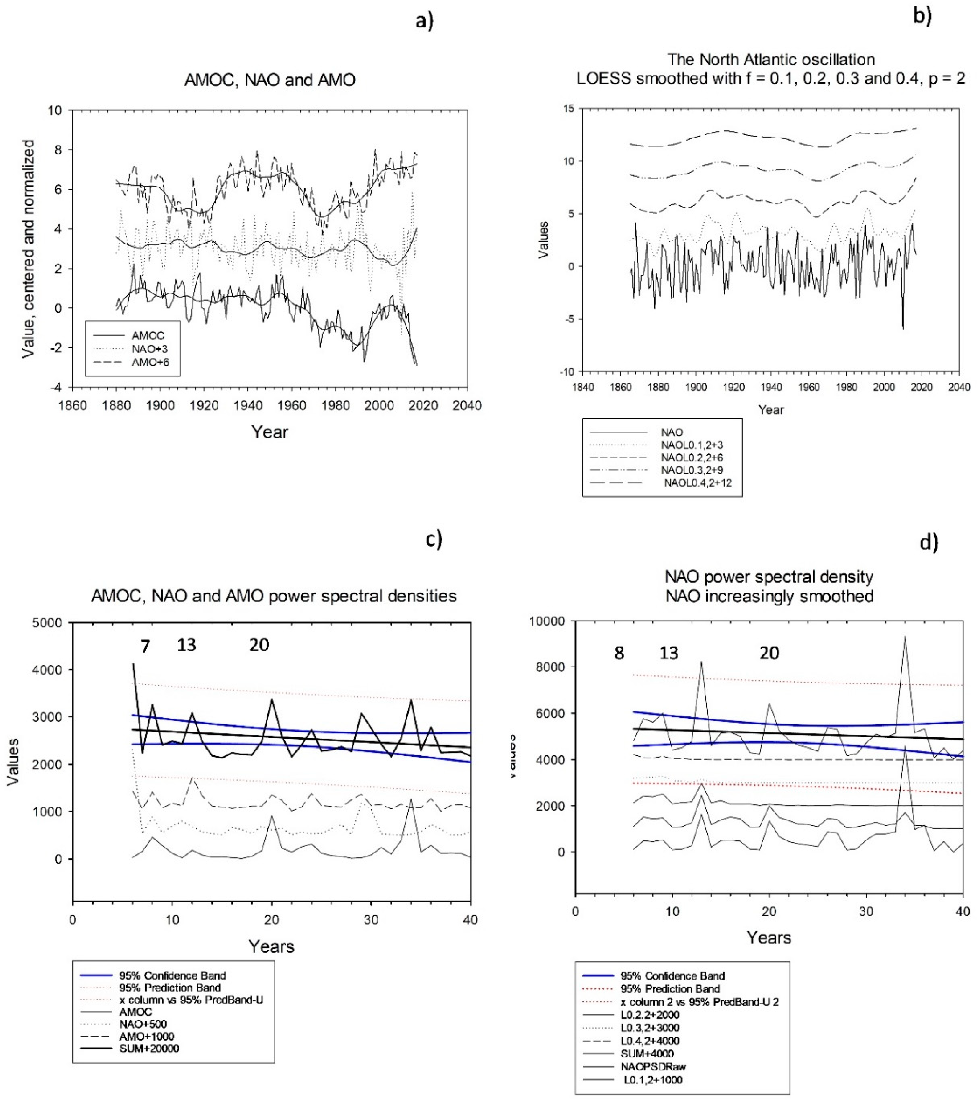
The three series are shown in Figure 1a,b. Smoothed versions are shown as thin lines superimposed on the raw time-series in Figure 1a, and in Figure 1b the NAO series are shown with increasing degree of smoothing. (See below on LOESS smoothing). Figure 1c,d will be discussed below.
In addition, we used a random generator, which gives a uniform distribution between 0 and 1. If points have normally distributed stochastic variation along an x-axis and an y-axis, then the angels between lines (xi, yi) and (xj, yj) and the x-axis are uniformly distributed on (−π/2, π/2), [25].
3. Methods
We first describe how we apply the PSD algorithm to the ocean oscillation time-series; thereafter we use a spectral stacking method to identify persistent peaks in the PSD curves. Second, we examine leading-lagging relations between paired time-series. Finally, we give an outline of the LOESS smoothing algorithm.
3.1. Stacking Method
The PSD algorithm identifies cycle times in cyclic time-series, often by identifying Fourier components in the series. Normally, PSD is applied to the whole time-series, but PSD may also be applied over rolling time windows.
To evaluate the results from the PSD, we use a multiple window method, e.g., Johnson, Thomson [3], but instead of using time windows drawn from the same time-series, we use (i) time-series that describe movement in the same ocean basins and (ii) time-series that are smoothed to an increasing degree. We do not fit any type of noise to the series, because random generators may produce periodic components [3]. By stacking the series, peaks that occur in all series will reinforce each other. For the stacked series, we calculate the 95% confidence interval for the model and the parameters. Peaks that breach the 95% confidence interval are potentially significantly periodic. Furthermore, the time-series for which the PSDs contribute to a peak in the average spectrum, probably reflect a real cycle in that time-series.
3.2. The LL-Method
We examine leading-lagging (LL) -relations between the NAO, the AMO and the AMOC. If the NAO is only white noise or a first order autoregressive AR(1) process, we would not anticipate to see a persistent LL-relation between the three oscillations. We first calculate the LL-relations between the three oscillation series, and thereafter we replace the NAO series with a uniformly random series and compare the result from this pairing to the first set of LL-relations.
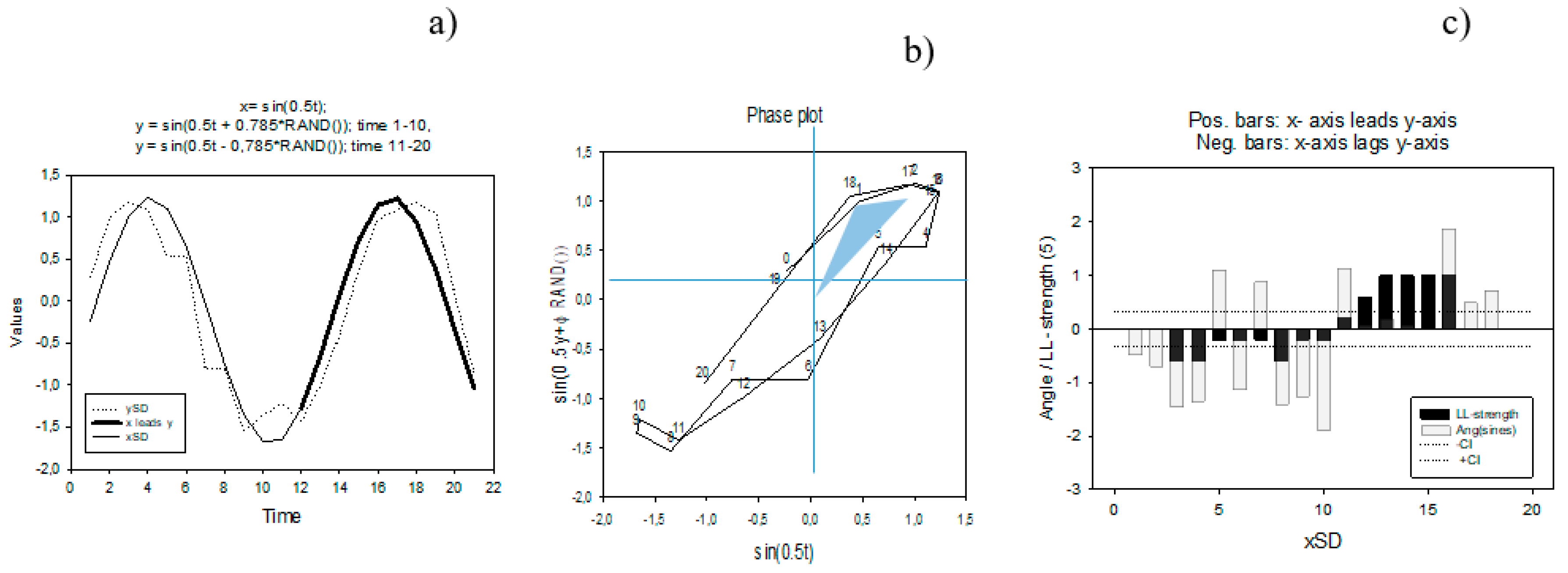
Leading-lagging relations. Leading-lagging relations between pairs of the NAO, the AMOC and the AMO time-series were identified by the leading–lagging (LL) -method of Seip and Grøn [6]. The LL-method is based on the rotational direction that paired time-series will show when plotted in a phase plot. Figure 2 gives a summary explanation of the method. A high LL-strength value means that the LL relations are persistent over several time steps > 5–11.
3.3. Sources of Variability in Ocean Time-series
Most time-series will be impacted by noise, in either an additive or a multiplicative mode, or something in between. Furthermore, series may include chaotic dynamics [26] especially if biological variables, like phytoplankton, play a role in modulating CO2 concentrations [27,28]. Furthermore, interaction between exogenous drivers and internal dynamics may produce peaks in the time-series that are neither associated with the driving function nor with internal dynamics [29].
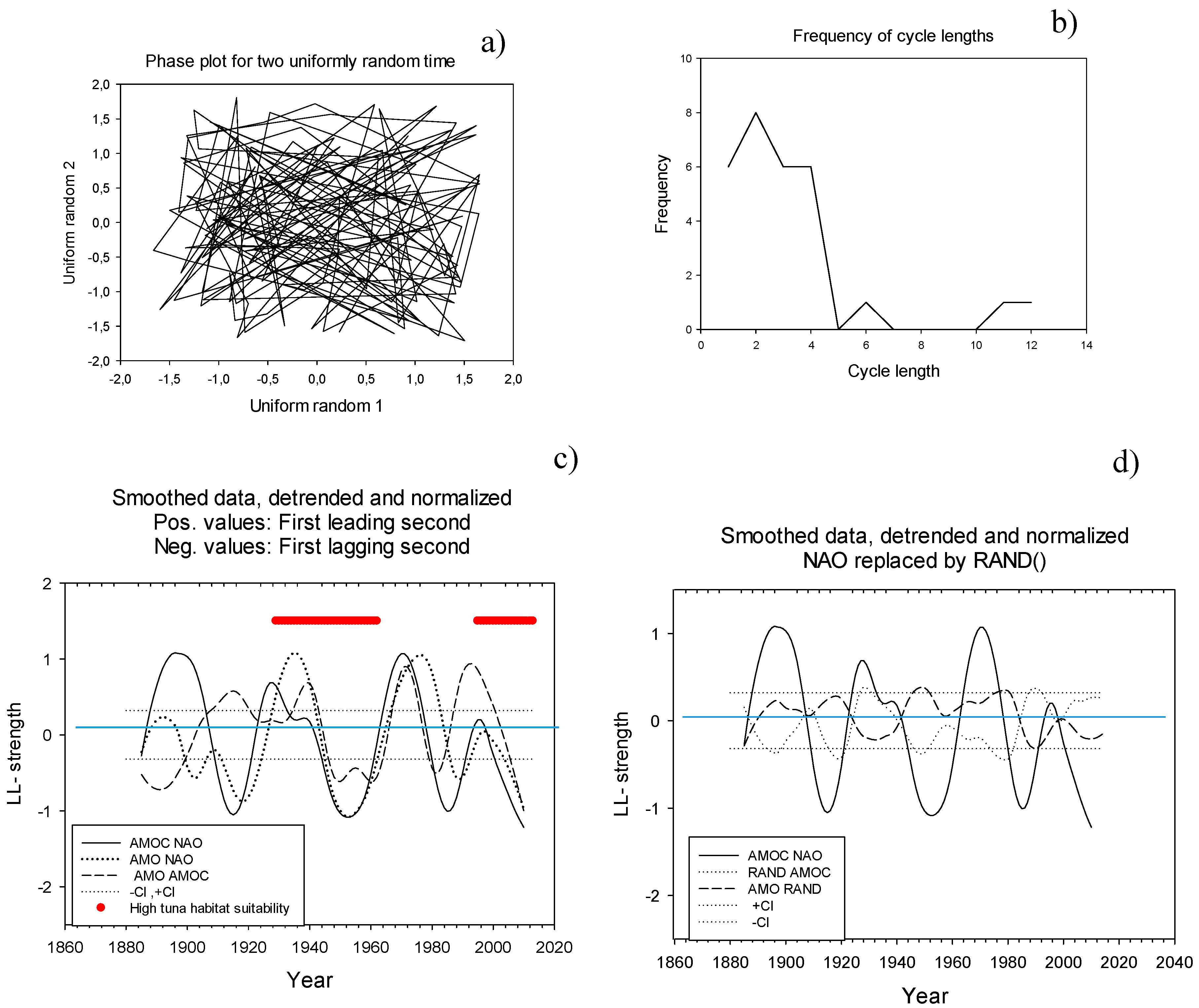
High frequencies. Noise, generated by natural variability, either by resampling, or with a random number generator may show periodic components. Johnson, Thomson [3] comment on periodic components in random generators, and Seip and Wang [5] show that in uniformly stochastic series, cycle frequencies lower than 5 may have a probability of more than 5% to occur by chance. This is shown in Figure 3a,b. We therefore removed the 5 first entries in the PSD series in Figure 1c,d. A graph similar to the one in Figure 3b is also found when card decks are shuffled to obtain a well-mixed deck [30,31].
Low frequencies. The lowest frequencies that can be established with confidence are in the range of 10% to 20% of the time-series length [1,32]. For the observed ocean time-series that are 130 years long, it means that cycles of more than 23 years (20%) will be uncertain. However, there might be other “sister” series that are longer, or there may be other types of information that suggest that time windows that are identified as trends are sections of time-series that oscillate. We made a cut off value at 40 years since several authors discuss features of the NAO that are 60 to 70 years long, but are not necessarily part of a cyclic series [4,17,33,34].
Smoothing. We smoothed the NAO series with the LOESS algorithm, SigmaPlot©, using fractions f = 0.1 to 0.4 of the series and a 2nd order polynomial function, (p) for interpolation.
4. Results
We first examine the three PSDs that describe ocean dynamics in the North Atlantic and thereafter the PSDs of the raw and smoothed NAO series. Last, we report the LL - relations between the three oscillations. Taken together, the results show that there are common characteristic oscillations in water movements of the Atlantic Ocean, and that the observed oscillations shifted between leading and lagging with 30 ± 11 years interval during the period 1880 to 2000.
4.1. The Three North Atlantic Ocean Dynamic Series
Figure 1a and c shows a comparison of time-series for the NAO, the AMO and the AMOC that all characterize the Atlantic Ocean. The NAO measures sea surface pressure difference between two locations whereas the AMO and the AMOC are constructed from several measures averaged over an area. Privalsky and Yushkov [1] suggest that averaging over large areas increases the signal to white noise ratio. We also LOESS smoothed the series to more clearly see trends or quasi cycles (f = 0.2, p = 2). We then calculated the LL-strength, n = 9 and finally LOESS smoothed the LL-strength values f = 0.2, p = 2. The series in Figure 1a appear to show that the NAO is closest to a white noise series. The AMO probably comes next, and the AMOC has the greatest signal to noise ratio. Figure 1c shows the PSD for the AMOC, the NAO and the AMO in the range of 5 to 40 years. The sum specter shows 7 peaks above the 95% confidence band. There are 5 peaks in the raw NAO series that are reinforced by PSDs of the other two series. The 7, 13 and 20 years cycles (read from the PSD numerical series) correspond to similar cycles in the two other series. A 26 years cycle may correspond to cycles in the range 29–32 years for the other two series and a cycle at 34 years may correspond to cycles at 34–36 years.
4.2. The NAO Series
Figure 1b shows the NAO with increasing degrees of smoothing. Figure 1d shows the PSD for the 5 versions of the NAO. By smoothing the series, we mimic an averaging process, which could occur if the series were obtained by sampling over larger regions.
The stacked NAO series (raw and LOESS smoothed with increasing degree of smoothing, f = 0.1 to 0.4, p = 2) showed a broad peak centered at 8 years, sharp peaks at 13 and 20 years, broader “humps” at 12–13 years, 20–21 years and 34–36 years, Figure 1d.
4.3. Leading-Lagging Relations between the Atlantic Oscillations
The results for the LL-relations between the three Atlantic oscillations are shown in Figure 3c. The results suggest that the three oscillation LL-relations: LL(AMOC, NAO), LL(AMO, NAO) and LL(AMO, AMOC) show concerted movements and describe different aspects of the same system of ocean dynamics. For the period 1920 to 2010, the Spearman rank correlation coefficient is in the range 0.5 to 0.7 and the probability value p is less than 0.0001. The cycle time results may extend into other ocean basins as well. Seip and Grøn [6] found dominating 7 years and 25 years cycles in tele-connections between NAO, the southern oscillation index (SOI), and the Pacific decadal oscillation (PDO).
The time between peaks in Figure 3c is 30 ± 11 years. The red lines in the figure show periods where Faillettaz, Beaugrand [4] find that tuna habitat suitability is high. To test whether the NAO series represent pure noise, we replaced the NAO series with a uniform stochastic series. The result then shows that there are no concerted movements and the pairs that include the random series vary within the confidence interval, Figure 3d.
4.4. LL-Relations and the Hiatus Period 1943 to 1975
The period 1943 to 1975 has been characterized as a hiatus period superimposed on an increasing trend of global warming. It is interesting that in the beginning of the hiatus period 1943 to 1975, the NAO is directly leading the AMOC and indirectly leading it via the AMO. (NAO → AMOC; NAO → AMO → AMOC.) At the end of the hiatus period, around 1975, the leading relations are reversed. For the full period 1880 to 2014 the NAO and the AMOC lead each other about an equal amount of time with 4–5 years lead lag times. (Significantly 50% of the time). The relations are pro-cyclic and counter cyclic about an equal number of times.
5. Discussion
Ocean oscillations tend to show several cycles [35] and these oscillations appear to be connected through oceanic and atmospheric “bridges” [7,35]. However, the cycles in one ocean region will often be shifted relative to another ocean region. To identify the cycles several methods have been used, from simple peak to peak measures and curve fitting methods [36] to PSD methods with added techniques to make the PSDs more robust relative to background noise and artefacts of the method.
To validate cycle times that are found with the various techniques, some climate time-series are extended, either by using proxy information, like tree-ring dating methods [20], or by using modeling tools [11]. However, in the present study we emphasize the original time-series.
We use three methods to validate candidate cycle length. First, we stack PSDs from several measures of cyclicity in the same ocean basin. The method is based on three assumptions, (i) the water movements in the ocean basin are governed by the same, or similar, mechanisms over the whole basin, (ii) by stacking the PSDs of different ocean oscillation time-series, signals that are common for the series will reinforce each other, whereas the others will annihilate each other, and (iii) if one series shows a signal (peak) which is present in the stacked PSD, it is also representative for the oscillation in the series it represents. Second, we stack increasingly smoothed versions of the same time-series, here, the NAO. Third, we examine LL-relations between pairs of the three ocean variable cycles, that is, we get three pairs of running LL-relations, NAO vs. AMO, NAO vs. AMOC and AMO vs. AMOC.
Among the three ocean cycle series that characterize the North Atlantic, the NAO is the one that appears to show the largest noise component. Still, the NAO may be a good description of ocean movements which impact climate variations in North Europe, e.g., Bardin and Polonsky [37] on winter cyclone frequencies in the Islandic low region and Faillettaz, Beaugrand [4] on Atlantic Bluefin tuna. We found that the NAO contributed to peaks in the PSD graphs for the Atlantic oscillation series at 7, 13, 19–20, 29–31 and 34–36 years. Furthermore, we find cycles at 7–8 years, 12–13 years and 20–21 years that also show up in the “sister” time-series of the North Atlantic. We do not yet know if the oscillations and the shift between them can be related to a see-saw or dipole pattern of heat transport in the North Atlantic, but Gastineau et al. [38] et al. find that both the NAO and the AMOC may play a role.
Gastineau et al. [38] compare model results and observations and find that low frequency variability in the AMOC strongly influences the seasonal variability of the NAO. Here we determine the dominating frequency at which these influences act. We found that Faillettaz, Beaugrand [4] show that the relative influence on Atlantic Bluefin tuna is 47.1% from AMO, and 21.5% from NAO (with a one-generation lag). Thus, both ocean oscillations contribute to the abundance of the tuna. The two oscillations act by the influence they have on the environmental temperature in the oceans, and the temperature again modulates recruitment and development of older stages of the stock. The shift in the sequences of temperatures favorable to tuna development may therefore be important for fishable stocks. This supports the argument by Faillettaz, Beaugrand [4] that climate variability must be taken into account in stock management plans.
Conventional methods for time-series analysis examine single time-series, and the series are often assumed to show stationarity. Here, we examine three series that are not stationary. The three series show some common, but also some distinct cycles. We suggest that the mechanisms that generate each cycles will be characteristic for the cycle examined. Such mechanisms are probably best studied with comprehensive models, e.g., as in Gastneau et al. [38]. The method we suggest is simple, but it relies on an understanding of the underlying system that the series are drawn from. In the present case, knowledge of large-scale oceanic water movements, their hydrodynamics and the laws that govern the hydrodynamics are important background information. We find that the NAO, the AMO and the AMOC show distinct cycles that closely reflect the Atlantic system they are part of, but they also show individual characteristics that may give clues to which atmospheric or oceanic mechanisms that generate them.
Author Contributions
Conceptualization, K.L.S., H.W. and Ø.G.; methodology, K.L.S.; software, K.L.S.; validation, K.L.S., H.W. and Ø.G.; formal analysis, K.L.S.; investigation, K.L.S. and H.W.; resources, All; data curation, All; writing—original draft preparation, K.L.S.; writing—review and editing, K.L.S., H.W. and Ø.G.; visualization, K.L.S.; supervision, K.L.S.; project administration, K.L.S.; funding acquisition, K.L.S.
Funding
This research received no external funding apart from support from Oslo Metropolitan University.
Acknowledgments
Data for the AMOC were kindly supplied by Levke Caesar, Potsdam Institute for Climate Impact Research.
Conflicts of Interest
The authors declare no conflict of interest.
References
- Privalsky, V.; Yushkov, V. Getting It Right Matters: Climate Spectra and Their Estimation. Pure Appl. Geophys. 2018, 175, 3085–3096. [Google Scholar]
- Mann, M.E.; Lees, J.M. Robust estimation of background noise and signal detection in climatic time series. Clim. Chang. 1996, 33, 409–445. [Google Scholar]
- Johnson, G.; Thomson, D.J.; Wu, E.X.; Williams, S.C.R. Multiple-window spectrum estimation applied to in vivo NMR spectroscopy. J. Magn. Reson. Ser. B 1996, 110, 138–149. [Google Scholar] [CrossRef]
- Faillettaz, R.; Beaugrand, G.; Goberville, E.; Kirby, R.R. Atlantic Multidecadal Oscillations drive the basin-scale distribution of Atlantic bluefin tuna. Sci. Adv. 2019, 5, 8. [Google Scholar] [CrossRef] [PubMed]
- Seip, K.L.; Wang, H. The hiatus in global warming and interactions between the El Niño and the Pacific decadal oscillation: comparing observations and modeling results. Climate 2018, 6, 18. [Google Scholar]
- Seip, K.L.; Grøn, Ø. Cycles in oceanic teleconnections and global temperature change. Theor. Appl. Climatol. 2018. [Google Scholar] [CrossRef]
- Alexander, M.A.; Bladé, I.; Newman, M.; Lanzante, J.R.; Lau, N.C.; Scott, J.D. The atmospheric bridge: The influence of ENSO teleconnections on air-sea interaction over the global oceans. J. Clim. 2002, 15, 2205–2231. [Google Scholar] [CrossRef]
- Vannitsem, S.; Ekelmans, P. Causal dependences between the coupled ocean-atmosphere dynamics over the tropical Pacific, the North Pacific and the North Atlantic. Earth Syst. Dyn. 2018, 9, 1063–1083. [Google Scholar] [CrossRef]
- Wu, S.; Liu, Z.; Zhang, R.; Delworth, T.L. On the observed relationship between the Pacific Decadal Oscillation and the Atlantic Multi-decadal Oscillation. J. Oceanogr. 2011, 67, 27–35. [Google Scholar] [CrossRef]
- Woollings, T.; Franzke, C.; Hodson, D.L.R.; Dong, B.; Barnes, E.A.; Raible, C.C.; Pinto, J.G. Contrasting interannual and multidecadal NAO variability. Clim. Dyn. 2015, 45, 539–556. [Google Scholar] [CrossRef]
- Knight, J.R.; Allan, R.J.; Folland, C.K.; Vellinga, M.; Mann, M.E. A signature of persistent natural thermohaline circulation cycles in observed climate. Geophys. Res. Lett. 2005, 32. [Google Scholar] [CrossRef]
- Nye, J.A.; Baker, M.R.; Bell, R.; Kenny, A.; Kilbourne, K.H.; Friedland, K.D.; Martino, E.; Stachura, M.M.; Van Houtan, K.S.; Wood, R. Ecosystem effects of the Atlantic Multidecadal Oscillation. J. Mar. Syst. 2014, 133, 103–116. [Google Scholar] [CrossRef]
- Alheit, J.; Drinkwater, K.F.; Nye, J.A. Introduction to Special Issue: Atlantic Multidecadal Oscillation-mechanism and impact on marine ecosystems. J. Mar. Syst. 2014, 133, 1–3. [Google Scholar] [CrossRef]
- Luterbacher, J.; Xoplaki, E.; Dietrich, D.; Rickli, R.; Jacobeit, J.; Beck, C.; Gyalistras, D.; Schmutz, C.; Wanner, H. Reconstruction of sea level pressure fields over the Eastern North Atlantic and Europe back to 1500. Clim. Dyn. 2002, 18, 545–561. [Google Scholar] [CrossRef]
- Hurrell, J.W. Decadal Trends in the North-Atlantic Oscillation—Regional Temperatures and Precipitation. Science 1995, 269, 676–679. [Google Scholar] [CrossRef]
- McCarthy, G.D.; Haigh, I.D.; Hirschi, J.J.M.; Grist, J.P.; Smeed, D.A. Ocean impact on decadal Atlantic climate variability revealed by sea-level observations. Nature 2015, 521, 508. [Google Scholar] [CrossRef]
- Jones, P.D.; Jonsson, T.; Wheeler, D. Extension to the North Atlantic Oscillation using early instrumental pressure observations from Gibraltar and south-west Iceland. Int. J. Climatol. 1997, 17, 1433–1450. [Google Scholar]
- Ortega, P.; Lehner, F.; Swingedouw, D.; Masson-Delmotte, V.; Raible, C.C.; Casado, M.; Yiou, P. A model-tested North Atlantic Oscillation reconstruction for the past millennium. Nature 2015, 523, 71. [Google Scholar]
- Kaplan, A.; Cane, M.A.; Kushnir, Y.; Clement, A.C.; Blumenthal, M.B.; Rajagopalan, B. Analyses of global sea surface temperature 1856–1991. J. Geophys. Res.-Ocean. 1998, 103, 18567–18589. [Google Scholar] [CrossRef]
- Gray, S.T.; Graumlich, L.J.; Betancourt, J.L.; Pederson, G.T. A tree-ring based reconstruction of the Atlantic Multidecadal Oscillation since 1567 AD. Geophys. Res. Lett. 2004, 31. [Google Scholar] [CrossRef]
- Rahmstorf, S.; Box, J.; Feulner, G.; Mann, M.E.; Robinson, A.; Rutherford, S.; Schaffernicht, E. Evidence for an exceptional twentieth-century slowdown in Atlantic Ocean overturning (vol 5, pg 475, 2015). Nat. Clim. Chang. 2015, 5, 956. [Google Scholar] [CrossRef]
- Caesar, L.; Rahmstorf, S.; Robinson, A.; Feulner, G.; Saba, V. Observed fingerprints of weakening Atlantic Ocean overturning circulation. Nature 2018, 556, 191–196. [Google Scholar] [CrossRef]
- Jackson, L.C.; Kahana, R.; Graham, T.; Ringer, M.A.; Woollings, T.; Mecking, J.V.; Wood, R.A. Global and European climate impacts of a slowdown of the AMOC in a high resolution GCM. Clim. Dyn. 2015, 45, 3299–3316. [Google Scholar] [CrossRef]
- Lynch-Stieglitz, J. The Atlantic Meridional Overturning Circulation and Abrupt Climate Change. Annu. Rev. Mar. Sci. 2017, 9, 83–104. [Google Scholar] [CrossRef]
- Seip, K.L.; Sas, H.; Vermij, S. The short term response to eutrophication abatement. Aquat. Sci. 1990, 52, 199–220. [Google Scholar] [CrossRef]
- Sugihara, G.; May, R.M. Nonlinear forecasting as a way of distinguishing chaos from measurement errors in time series. Nature 1990, 344, 731–741. [Google Scholar] [CrossRef]
- Tømte, O.; Seip, K.L.; Christophersen, N. Evidence That Loss in Predictability Increases with Weakening of (Metabolic) Links to Physical Forcing Functions in Aquatic Ecosystems. Oikos 1998, 82, 325–332. [Google Scholar] [CrossRef]
- Hsieh, C.H.; Glaser, S.M.; Lucas, A.J.; Sugihara, G. Distinguishing random environmental fluctuations from ecological catastrophes for the North Pacific Ocean. Nature 2005, 435, 336–340. [Google Scholar] [CrossRef]
- Seip, K.L.; Pleym, H. Competition and predation in a seasonal world. Internationale Vereinigung für Theoretische und Angewandte Limnologie 2000, 27, 823–827. [Google Scholar] [CrossRef]
- Mann, B. How many times should you shuffle a deck of cards? Umap J. 1994, 4, 303–332. [Google Scholar]
- Bayer, D.; Diaconis, P. Trailing the dovetail shuffle to its lair. Ann. Appl. Probab. 1992, 2, 294–313. [Google Scholar] [CrossRef]
- Ghil, M.; Allen, M.R.; Dettinger, M.D.; Ide, K.; Kondrashov, D.; Mann, M.E.; Robertson, A.W.; Saunders, A.; Tian, Y.; Varadi, F.; et al. Advanced spectral methods for climatic time series. Rev. Geophys. 2002, 40. [Google Scholar]
- Delworth, T.L.; Zeng, F.; Zhang, L.; Zhang, R.; Vecchi, G.A.; Yang, X. The Central Role of Ocean Dynamics in Connecting the North Atlantic Oscillation to the Extratropical Component of the Atlantic Multidecadal Oscillation. J. Clim. 2017, 30, 3789–3805. [Google Scholar] [CrossRef]
- Mazzarella, A.; Scafetta, N. Evidences for a quasi 60-year North Atlantic Oscillation since 1700 and its meaning for global climate change. Theor. Appl. Climatol. 2012, 107, 599–609. [Google Scholar] [CrossRef]
- Newman, M.; Shin, S.I.; Alexander, M.A. Natural variation in ENSO flavors. Geophys. Res. Lett. 2011, 38. [Google Scholar] [CrossRef]
- Wu, Z.H.; Huang, N.E.; Wallace, J.M.; Smoliak, B.V.; Chen, X. On the time-varying trend in global-mean surface temperature. Clim. Dyn. 2011, 37, 759–773. [Google Scholar]
- Bardin, M.Y.; Polonsky, A.B. North Atlantic oscillation and synoptic variability in the European-Atlantic region in winter. Izv. Atmos. Ocean. Phys. 2005, 41, 127–136. [Google Scholar]
- Gastineau, G.; D’Andrea, F.; Frankignoul, C. Atmospheric response to the North Atlantic Ocean variability on seasonal to decadal time scales. Clim. Dyn. 2013, 40, 2311–2330. [Google Scholar] [CrossRef]
Figure 1.
Time-series and their power spectral densities. (a) Time-series for the AMOC, the NAO and the AMO, the full lines are LOESS (0.2, 2) smoothed versions; (b) Time-series for NAO, LOESS smoothed to different degrees. (c) Power spectral density for the AMOC, the NAO and the AMO and the three series superimposed. The three series show common pronounced peaks at 7 years 13 years, 19–20 years, 23–24 years, and 34–36 years; (d) Power spectral density for the NAO at different LOESS smoothing degrees. The time-series show pronounced peaks at 7–9 years, 13 years, 16 years, 20 years, 26–27 years, and 34–36 years.

Figure 2.
Example. Calculating leading-lagging (LL) relations and LL–strength. (a) Two sine functions: the smooth curve is a simple sine function, sin (0.5t), the dashed curve has the form sin (0.5t + ϕ × RAND()) where ϕ = +0.785 for t = 1–10 and ϕ = −0.785 for t = 11–20. RAND() is the Excel random generator. Bold part of the simple sine function, xSd shows that it leads ySD. (b) In a phase plot with sin (0.5.t) on the x-axis and the sin(0.5t + ϕ × RAND()) on the y-axis, the time-series rotates first clock-wise (1 to 10, negative by definition) then counter clock wise 11 to 20; θ is the angle between two consecutive trajectories. The wedge suggests the angle between the origin and lines to observations 1 and 2. (c) Angles between successive trajectories (grey bars) and LL-strength (black bars). LL-strength allows some outliers from a persistent pattern. Dashed lines suggest confidence limits for persistent rotation in the phase plot and persistent leading or lagging relations in the time-series plot.

Figure 3.
Cycle times and leading-lagging relations. (a) Phase plot for two uniform random series, (b) Rotations in phase plot that complete a full circle, that is, angles add to 2 π. A similar figure to Figure 3b occurs when the calculations are repeated 100 times. (c) Leading-lagging relations between the NAO, the AMOC and the AMO. Figure from Seip and Grøn [6], their supplementary material. Raw series LOESS smoothed f = 0.2, p = 2; LL- relations LOESS smoothed f = 0.2, p = 2. Cycle time for the smoothed series are 21 to 24 years and leading - lagging time 5 to 6 years. Red liners show high tuna habitat suitability in accordance with reference [4]. (d) Leading-lagging relations between NAO replaced by the uniform random generator RAND(), and the AMOC and the AMO.

© 2019 by the authors. Licensee MDPI, Basel, Switzerland. This article is an open access article distributed under the terms and conditions of the Creative Commons Attribution (CC BY) license (http://creativecommons.org/licenses/by/4.0/).
Share and Cite
MDPI and ACS Style
Seip, K.L.; Grøn, Ø.; Wang, H. The North Atlantic Oscillations: Cycle Times for the NAO, the AMO and the AMOC. Climate 2019, 7, 43. https://0-doi-org.brum.beds.ac.uk/10.3390/cli7030043
AMA Style
Seip KL, Grøn Ø, Wang H. The North Atlantic Oscillations: Cycle Times for the NAO, the AMO and the AMOC. Climate. 2019; 7(3):43. https://0-doi-org.brum.beds.ac.uk/10.3390/cli7030043
Chicago/Turabian StyleSeip, Knut Lehre, Øyvind Grøn, and Hui Wang. 2019. "The North Atlantic Oscillations: Cycle Times for the NAO, the AMO and the AMOC" Climate 7, no. 3: 43. https://0-doi-org.brum.beds.ac.uk/10.3390/cli7030043
Note that from the first issue of 2016, this journal uses article numbers instead of page numbers. See further details here.